경험 재생에서 깊은 망각과 얕은 망각의 비대칭: 작은 버퍼는 특징 공간을 유지하지만 분류 경계는 왜곡한다

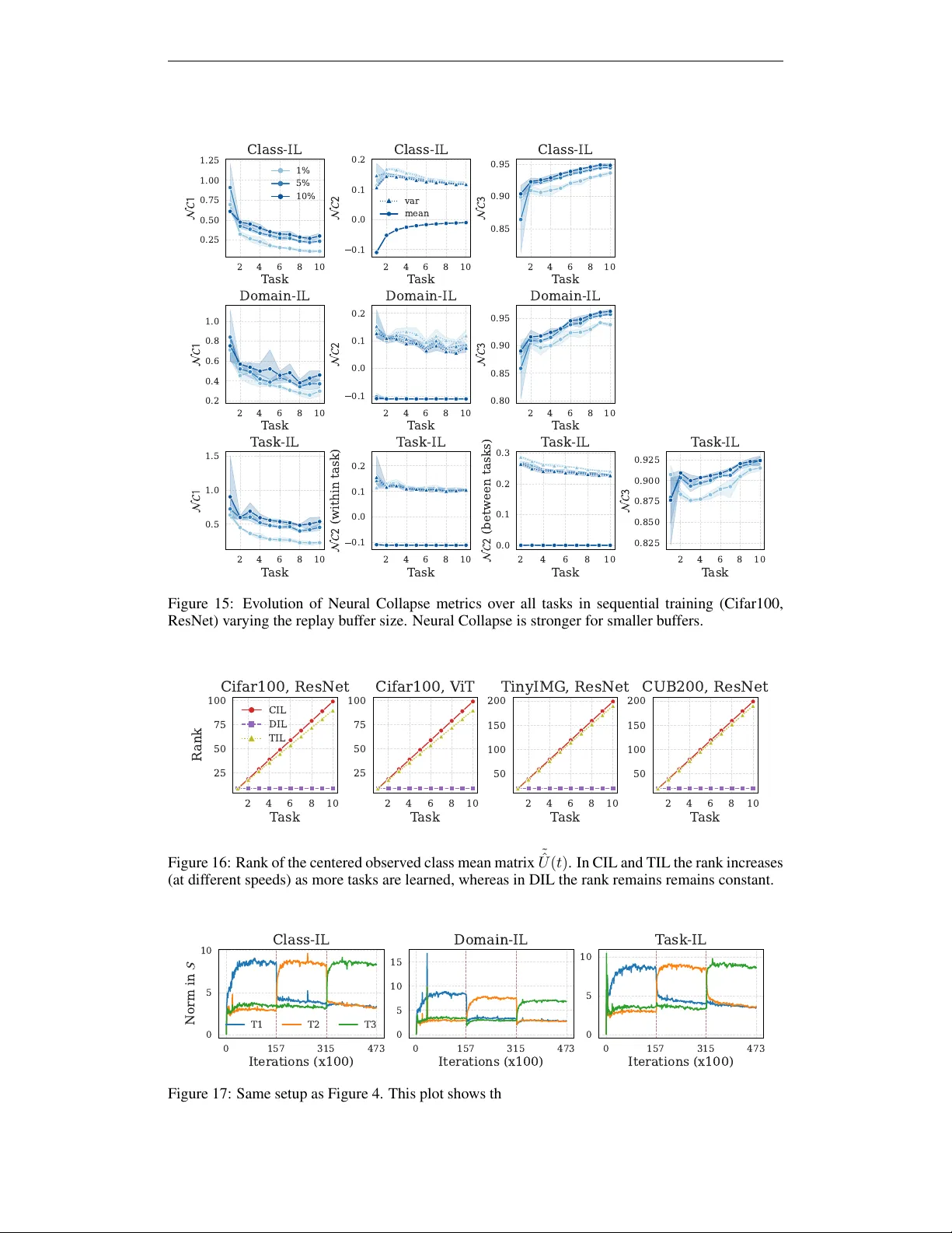
Preprint. A S Y M P T O T I C A N A L Y S I S O F S H A L L O W A N D D E E P F O R - G E T T I N G I N R E P L A Y W I T H N E U R A L C O L L A P S E Giulia Lanzillotta ∗ , Damiano Meier ∗ & Thomas Hofmann ETH AI Center & Department of Computer Science, ETH Z ¨ urich A B S T R AC T A persistent paradox in continual learning (CL) is that neural networks often retain linearly separable representations of past tasks ev en when their out- put predictions fail. W e formalize this distinction as the gap between deep (feature-space) and shallow (classiﬁer-le vel) forgetting. W e rev eal a critical asymmetry in Experience Replay: while minimal buf fers successfully anchor feature geometry and prevent deep forgetting, mitigating shallow forgetting typically requires substantially lar ger b uffer capacities. T o e xplain this, we extend the Neural Collapse frame work to the sequential setting. W e characterize deep forgetting as a geometric drift to ward out-of-distrib ution subspaces and prove that any non-zero replay fraction asymptotically guarantees the retention of linear separability . Con versely , we identify that the ”strong collapse” induced by small buf fers leads to rank-deﬁcient co variances and inﬂated class means, effecti vely blinding the classiﬁer to true population boundaries. By unifying CL with out-of-distribution detection, our work challenges the prev ailing reliance on large buf fers, suggesting that explicitly correcting these statistical artifacts could unlock robust performance with minimal replay . T asks T ask onset Good buf fer boundary Good population boundary Area of Buf fer - optimal decision boundaries The data is OOD, there is no class information in the features Classes are separable Classes are still separable but the the decision boundary is misaligned Shallow Forgetting Figure 1: Evolution of decision boundaries and featur e separability . PCA ev olution of two Cifar10 classes (1% replay). Replay samples are highlighted with a black edge. While features retain separability across tasks (low deep forgetting), the classiﬁer optimization becomes under- determined : multiple ”buf fer-optimal” boundaries (dashed bro wn) perfectly classify the stored sam- ples b ut largely fail to align to the true population boundary (dashed green), resulting in shallow forgetting. 1 I N T R O D U C T I O N Continual learning (Hadsell et al., 2020) aims to train neural networks on a sequence of tasks with- out catastrophic forgetting. It holds particular promise for adapti ve AI systems, such as autonomous agents that must integrate new information without full retraining or centralized data access. The theoretical understanding of optimization in non-stationary environments remains limited, particu- larly regarding the mechanisms that go vern the retention and loss of learned representations. A persistent observation in the literature is that neural networks retain substantially more information about past tasks in their internal representations than in their output predictions. This phenomenon, ∗ Corresponding authors, email at { glanzillo,dammeier } @ethz.ch . 1 Preprint. ﬁrst demonstrated through linear pr obe evaluations , shows that a linear classiﬁer trained on frozen last-layer representations achie ves markedly higher accurac y on old tasks than the network’ s own output layer (Murata et al., 2020; Hess et al., 2023). In other words, past-task data remain linearly separable in feature space, ev en when the classiﬁer fails to exploit this structure. This motiv ates a distinction between two levels of forgetting: shallow f orgetting , corresponding to output-lev el degradation recoverable by a linear probe, and deep f orgetting , corresponding to irre versible loss of feature-space separability . In this work, we show that r eplay b uffers af fect these two forms of for getting in systematically dif fer- ent ways . Replay—the practice of storing a small subset of past samples for joint training with new data—is among the most effecti ve and widely adopted strate gies in continual learning. Howe ver , the requirement to store and repeatedly process substantial amounts of past data limits its scalabil- ity . Our analysis re veals a critical ef ﬁciency gap: even small b uffers ar e sufﬁcient to pr eserve featur e separability and pr event deep for getting , whereas mitigating shallow for getting requires substan- tially larger buf fers. Thus, while replay robustly preserves representational geometry , it often fails to maintain alignment between the learned head and the true data distribution. T o e xplain this phenomenon, we turn to the geometry of deep network representations. Recent work has shown that, at con vergence, standard architectures often exhibit highly structured, low- dimensional feature or ganization. In particular , the Neur al Collapse (NC) phenomenon (P apyan et al., 2020) describes a regime in which within-class variability vanishes, class means form an equiangular tight frame (ETF), and classiﬁer weights align with these means. Originally observed in simpliﬁed settings, NC has now been documented across architectures, training regimes, and ev en large-scale language models (S ´ uken ´ ık et al., 2025; W u & Pap yan, 2025), making it a powerful framew ork to analyze feature-head interactions. In this w ork, we extend the NC frame work to continual learning, pro viding a characterization of the geometry of features and heads under extended training. Our analysis covers task-, class-, and domain-incremental settings and explicitly accounts for replay . T o account for this, we propose two governing hypotheses for historical data absent from the buf fer: (1) topologically , forgotten samples behave as out-of-distribution (OOD) entities, and (2) enlarging the replay buf fer induces a smooth interpolation between this OOD regime and fully collapsed representations. These insights allow us to construct a simple yet predicti ve theory of feature-space forgetting that lower -bounds separability and captures the inﬂuence of weight decay , feature-norm scaling, and buf fer size. In summary , this paper makes the following distinct contrib utions: 1. The r eplay efﬁciency gap. W e identify an intrinsic asymmetry in replay-based contin- ual learning: minimal buf fers are suf ﬁcient to anchor feature geometry (prev enting deep forgetting), whereas mitigating classiﬁer misalignment (shallow forgetting) requires dis- proportionately large capacities. 2. Asymptotic framework for continual learning. W e e xtend Neural Collapse theory to continual learning, characterizing the asymptotic geometry of both single-head and multi-head architectures and identifying unique phenomena like rank reduction in task- incremental learning. 3. Effects of r eplay on feature geometry . W e demonstrate that shallo w for getting arises because classiﬁer optimization on buf fers is under-determined —a condition structurally exacerbated by Neural Collapse . The resulting geometric simpliﬁcation (cov ariance deﬁ- ciency and norm inﬂation) blinds the classiﬁer to the true population boundaries. 4. Connection to OOD detection. W e reconceptualize deep forgetting as a geometric drift to- ward out-of-distrib ution subspaces. This perspectiv e bridges the gap between CL and OOD literature, offering a rigorous geometric deﬁnition of ”forgetting” beyond simple accuracy loss. 1 . 1 N O TA T I O N A N D S E T U P W e adopt the standard compositional formulation of a neural network, decomposing it into a feature map and a classiﬁcation head. The network function is deﬁned as f θ ( x ) = h ( ϕ ( x )) , where h ( z ) = W h z + b h , with parameters θ = { ϕ, W h } . 2 Preprint. W e refer to ϕ as the feature map , to its image as the featur e space and to ϕ ( x ) as the featur es or r epr esentation of input x . W e consider sequential classiﬁcation problems subdivided into tasks. For each class c , a dataset of labeled e xamples ( X c , Y c ) is av ailable for training. Giv en an y sample ( x, y ) , the netw ork prediction is obtained via the maximum-logit rule ˆ y = arg max k ⟨ w k , ϕ ( x ) ⟩ , where w k denotes the k -th column vector of W h . Network performance is ev aluated after each task on all previously seen tasks. Follo wing Lopez-Paz & Ranzato (2017), shallow forg etting is quantiﬁed as the dif ference A ij − A j j , where A ij denotes the accuracy on task j measured after completing learning session i . In contrast, deep for getting is deﬁned as the dif ference A ⋆ ij − A ⋆ j j , where A ⋆ ij represents the accuracy of a linear pr obe trained on the frozen representations of task j at the end of session i . W e adopt the three continual learning setups introduced by van de V en et al. (2022), described in detail in Section 3: task-incr emental learning (TIL), class-incr emental learning (CIL), and domain-incr emental learning (DIL). For the experimental analysis, we train both ResNet and V iT architectures, from scratch and from a pre-trained initialization. W e train on three widely used benchmarks adapted to the continual learning setting: Cifar100 (Krizhe vsky & Hinton, 2009), T iny-ImageNet (T orralba et al., 2008), and CUB200 (W ah et al., 2011). A detailed description of datasets and training protocols, including linear probing, is provided in Section A.1. 2 E M P I R I C A L C H A R AC T E R I Z A T I O N O F D E E P A N D S H A L L O W F O R G E T T I N G 0 2 4 6 8 10 100 Buf fer size (%) 0 20 40 60 80 F or getting Cifar100, ResNet 0 2 4 6 8 10 100 Buf fer size (%) 0 20 40 60 80 100 Cifar100, V iT 0 2 4 6 8 10 100 Buf fer size (%) 0 20 40 60 80 T inyIMG , ResNet 0 2 4 6 8 10 100 Buf fer size (%) 0 20 40 60 80 CUB200, ResNet shallow deep CIL DIL TIL Pr etrained Pr etrained Figure 2: Replay efﬁciency gap. Forgetting decays at different rates in the feature space and the classiﬁer head, producing a persistent gap between deep and shallow forgetting. Increasing the replay buf fer closes this gap only gradually , with substantial buffer sizes required for con ver gence. See Section A.2 for details. W e ﬁrst present our main empirical ﬁnding. W e ev aluate for getting in both the netw ork output layer and a linear probe trained on frozen features across v arying b uffer sizes, datasets, and architec- tures (randomly initialized and pre-trained). Our results, summarized in Figure 2, re veal a robust phenomenon: while small replay buffers ar e sufﬁcient to prevent deep forgetting (pr eserving feature separability), mitigating shallow forgetting requires substantially larger buffers . This extends prior observ ations of feature-output discrepancies (Murata et al., 2020; Hess et al., 2023) by demonstrating that r eplay stabilizes r epr esentations far more efﬁciently than it maintains classiﬁer alignment . The gap persists across settings, vanishing only near full replay (100%). W e highlight three speciﬁc trends: 1. Head arc hitectur e. The deep–shallow gap is pronounced in single-head setups (CIL, DIL) but signiﬁcantly smaller in multi-head setups (TIL). 2. Replay efﬁcacy in DIL. Contrary to the assumption that CIL is the most challenging bench- mark, DIL exhibits high le vels of deep for getting, con verging to le vels similar to CIL. 3 Preprint. 3. Pre-tr aining r obustness. Corroborating Ramasesh et al. (2021), pre-trained models exhibit negligible deep for getting. Their feature spaces remain rob ust even with minimal replay , yielding nearly ﬂat deep-forgetting curv es. In the following section, we present a theoretical model explaining this asymmetric effect of replay via the asymptotic dynamics of the feature space. 3 N E U R A L C O L L A P S E U N D E R S E Q U E N T I A L T R A I N I N G 3 . 1 P R E L I M I N A R I E S O N N E U R A L C O L L A P S E Recent work (Papyan et al., 2020; Lu & Steinerberger, 2022) characterizes the geometry of repre- sentations in the terminal phase of training (TPT) the regime in which the training loss has reached zero and features stabilize. In this regime, features con verge to a highly symmetric conﬁguration known as Neural Collapse (NC), which is prov ably optimal for standard supervised objectives and emerges naturally under a range of optimization dynamics (Tirer & Bruna, 2022; S ´ uken ´ ık et al., 2025). W e denote the feature class means by µ c ( t ) = E x ∈ X c [ ϕ t ( x )] , ˜ µ c ( t ) the centered means, and the matrix of centered means by ˜ U ( t ) . W e focus on ﬁrst three properties deﬁning NC: • N C 1 (V ariability Collapse). Within-class v ariability v anishes as features collapse to their class means: ϕ t ( x ) → µ c ( t ) , ∀ x ∈ X c , implying the within-class covariance approaches 0 . • N C 2 (Simplex ETF). Centered class means form a simplex Equiangular Tight Frame (ETF). They attain equal norms and maximal pairwise separation: lim t →∞ ⟨ ˜ µ c ( t ) , ˜ µ c ′ ( t ) ⟩ = ( β t if c = c ′ − β t K − 1 if c  = c ′ • N C 3 (Neural Duality). Classiﬁer weights align with the class means up to scaling, i.e., W ⊤ h ( t ) ∝ ˜ U ( t ) . 3 . 2 N E U R A L C O L L A P S E I N C O N T I N UA L L E A R N I N G Standard e valuation in continual learning measures performance strictly at the completion of each task. Thus, while forgetting arises from optimization dynamics, its magnitude is deﬁned effecti vely by the network’ s conﬁguration at the end of training. W e leverage the Neural Collapse framework to rigorously characterize this terminal geometry , modeling the stable structures that emerge in the limit of long training times. 1 While prior work focuses on stationary settings, we extend the NC framew ork to continual learning. W e empirically verify its emergence in domain- (DIL), class- (CIL), and task-incremental (TIL) settings (Figure 3, see Section C.4). Observed vs. population statistics. NC emerges on the training data (current task + buf fer). W e must therefore distinguish between observed statistics ˆ µ (computed on av ailable training samples) and population statistics µ (computed on the full distrib ution). The following empirical analysis concerns ˆ µ ; in subsequent sections, we dev elop a theory for µ to quantify forgetting. 3 . 2 . 1 S I N G L E - H E A D A R C H I T E C T U R E S In domain-incr emental learning (DIL) , all tasks share a ﬁxed label set, with each task introducing a ne w input distribution. Consequently , while the estimated class means ˆ µ c and global mean ˆ µ G ev olve throughout the task sequence, the asymptotic target geometry remains in variant: the number of class means and their optimal angles are constant. W e ﬁnd that the NC properties established in 1 Our analysis focuses on structures at con vergence; howe ver , we observ e that Neural Collapse emerges quickly in practice across standard architectures (cf. Figure 3). 4 Preprint. Class-IL T1 T2 T3 Domain-IL 0 157 314 472 Iterations (x100) T ask -IL 0 157 314 472 Iterations (x100) between tasks 0 157 314 472 Iterations (x100) Optimum = 1 - K-1 Optimum = 0 Optimum = 1 1 - 30-1 1 - 10-1 1 - 10-1 1 - 10-1 1 - 20-1 - 0.10 - 0.05 0.00 - 0.10 - 0.05 0.00 - 0.10 - 0.05 0.00 0.00 0.50 1.00 0.00 0.50 1.00 0.00 0.50 1.00 0 5 10 0 5 10 0 5 10 Figure 3: NC metrics in sequential training (Cifar100, ResNet with 5% replay). NC emerges across all tasks. In DIL, the ETF structure ( N C 2 ) remains stable; in CIL, it evolv es as class count increases; in TIL, it arises per-head with variable cross-task alignment. Highlighted in green is the asymptotic limit of the NC metrics. See Section A.2 for details. the single-task regime (Deﬁnitions 4 to 6) persist under DIL. When a replay buf fer is employed, the class means are effecti vely computed o ver the mixture of ne w data and buf fered samples. In class-incremental lear ning (CIL) , each task introduces a disjoint subset of classes. The asymp- totic structure of the feature space is therefore redeﬁned after each task, governed by the relative representation of old versus ne w classes. When past classes are under-represented in the training dataset, they act as minority classes : their features collapse toward a degenerate distrib ution centered near the origin, and their classiﬁer weights con ver ge to constant vectors (Fang et al., 2021; Dang et al., 2023). This phenomenon, known as Minority Collapse (MC), occurs sharply below a critical representation threshold. Without replay , MC dominates the asymptotic structure as past classes are absent from the loss. Howe ver , we observe that replay mitigates this ef fect when buf fers are sampled in a task-balanced manner . This strategy ensures that all classes—both new and old—are equally represented in each training batch, thereby preserving the global ETF structure and prev enting the marginalization of past tasks (Figure 3). 3 . 2 . 2 M U LT I - H E A D A R C H I T E C T U R E S Neural Collapse has not previously been characterized in multi-head architectures. In task- incremental learning (TIL) , the network output is partitioned into separate heads, each associated with a distinct task. This ensures that error propagation is localized to the assigned head (see Fig- ure 25). While this local normalization pre vents Minority Collapse ev en without replay , the resulting global geometry across tasks is non-trivial. Speciﬁcally , we in vestigate the relati ve angles and norms between class means belonging to different tasks. W e measure standard NC metrics including within-class variance, inter-task inner products, and feature norms. Our ﬁndings rev eal a clear distinction between local and global structure in TIL: 1. Local collapse. NC emerges consistently within each head. Each task-speciﬁc head satisﬁes N C 1 – N C 3 locally . 2. Global misalignment. A coherent cross-task NC structure is absent. Across tasks, class means display variable scaling and alignment (Figure 3, Figures 12 to 14 ). 3. Rank reduction. W e ﬁnd that local normalization induces a dimensionality reduction in the feature space. The global feature space attains a maximal rank of n ( K − 1) for n tasks, which is strictly lower than the nK − 1 rank observed in single-head settings (Figure 16). These empirical observations—speciﬁcally that task-balanced replay restores global NC in single- head setups while TIL lacks global alignment—serve as the foundation for the theoretical model of class separability dev eloped in the next section. 5 Preprint. 4 A S Y M P T O T I C B E H A V I O U R O F D E E P A N D S H A L L O W F O R G E T T I N G 4 . 1 P R E L I M I N A R I E S Linear separability . T o analyse deep forgetting, we require a mathematically tractable measure of linear separability in feature space. Formally , linear separability between two distributions P 1 and P 2 is the maximum classiﬁcation accuracy achiev able by any linear classiﬁer . Given the ﬁrst two moments ( µ 1 , Σ 1 ) and ( µ 2 , Σ 2 ) , the Mahalanobis distance is a standard proxy . Here, we use the signal-to-noise ratio (SNR) between class distrib utions, deﬁned as S N R ( c 1 , c 2 ) = ∥ µ 1 − µ 2 ∥ 2 T r(Σ 1 + Σ 2 ) . Higher SNR values imply greater separability . In Section C.2, we show that this quantity lo wer- bounds the Mahalanobis distance, and thus linear separability itself. Accordingly , we focus on the ﬁrst- and second-order statistics of class representations (means and covariances), as these directly gov ern the SNR. Asymptotic notation. W e use O ( · ) and Θ( · ) to characterize the scaling of time-dependent quan- tities f ( t ) , suppressing constants independent of t . When bounds depend on controllable quantities such as the buf fer size b , we retain these dependencies e xplicitly . This notation highlights scaling behaviour rele v ant to training dynamics and experimental design choices. 4 . 2 A N A LY S I S O F D E E P F O R G E T T I N G 4 . 2 . 1 F O R G OT T E N ≈ O U T - O F - D I S T R I B U T I O N 0 157 315 473 Iterations (x100) 0 5 10 N o r m i n T1 T2 T3 Figure 4: Projection of ˜ µ c ( t ) onto S t (Cifar100, no replay) . The population means of past and fu- ture tasks exhibit equiv alent (near- zero) norms when projected onto the activ e subspace S t . The Neural Collapse (NC) framew ork characterizes the asymptotic geometry of representations for training data. For- getting, ho wev er , concerns the ev olution of representations for samples of past tasks that are no longer part of the optimization objectiv e. W e bridge this conceptual gap through the follo wing hypothesis: Hypothesis 1. For gotten samples beha ve analogously to sam- ples that were nev er learned, i.e., they are effecti vely out-of- distribution (OOD) with respect to the current model. This perspecti ve moti vates our analysis of for getting as a form of shift to out-of-distribution in feature space. Speciﬁcally , in the absence of replay , data from past tasks e xhibits the same geometric behaviour as future-task (OOD) inputs. T o formal- ize this correspondence, we adopt a feature-space deﬁnition of OOD based on the recently proposed ID/OOD orthogonality property ( NC5 , Ammar et al., 2024). Deﬁnition 1 (Out-of-distribution (OOD)) . Let X c denote the samples of class c , and let ϕ t ( x ) be the feature map of a network trained on dataset D with K classes. Denote by S t = span { ˜ ˆ µ 1 ( t ) , . . . , ˜ ˆ µ K ( t ) } the active subspace spanned by the center ed class means of the training data at time t . W e say that X c is out-of-distribution for ϕ t if the average representation of X c is orthogonal to S t . In Section C.6 (Proposition 2), we sho w that, under the NC regime, the empirical observation that OOD inputs yield higher predictive entropy than in-distrib ution (ID) inputs is mathematically equi v- alent to this orthogonality condition—thus establishing a formal connection between predictiv e un- certainty and the geometric structure of NC5. W e validate our hypothesis by monitoring the projection of centered class means ˜ µ c onto the active subspace S t . As sho wn in Figure 4 (and Figures 17 to 19), shortly after a task switch, the projection of past-task means collapses sharply , indistinguishably matching the behavior of unseen (OOD) tasks. 6 Preprint. 4 . 2 . 2 A S Y M P T OT I C D I S T R I B U T I O N O F O O D C L A S S E S Lev eraging the connection between forgetting and OOD dynamics, we no w characterize the asymp- totic behavior of past-task data. W e ﬁnd that the residual signal of past classes is conﬁned to the inactive subspace S ⊥ , making it susceptible to erasure by weight decay . Theorem 1 (Asymptotic distribution of OOD data) . Let X c be OOD inputs (Deﬁnition 1) for a featur e map ϕ t trained with a sufﬁciently small learning rate η and weight decay λ . Let β t denote the observed center ed class-mean norm as by Deﬁnition 5. In the terminal phase ( t ≥ t 0 ), the featur e distribution of X c has mean µ c and variance σ 2 c given by: µ c ( t ) = (1 − η λ ) t − t 0 µ c,S ⊥ ( t 0 ) , (1) σ 2 c ( t ) ∈ Θ  β t + (1 − η λ ) 2( t − t 0 )  . (2) Corollary 1 (Collapse to null distribution) . If λ > 0 , the OOD distribution con verg es to a de gener- ate null distribution: the mean decays to zer o, and the variance limits depend on β t . The proof (see Theorem 4) relies on the observation that, once N C 3 (alignment between class fea- ture means and classiﬁer weights) emerges, optimization updates become r estricted to the active subspace S t . Consequently , components of the representation in the orthogonal complement S ⊥ t are frozen—or decay exponentially under weight decay— yielding the dynamics abo ve. ☞ Notation. For bre vity , let υ = 1 − η λ , and note that S t = S t 0 = S for all t ≥ t 0 . Theorem 2 (Lower bound on OOD linear separability) . F or two OOD classes c, c ′ in the TPT , let υ = 1 − η λ . The Signal-to-Noise Ratio (SNR), which lower -bounds linear separability , satisﬁes: SNR( c, c ′ ) ∈ Θ  β t υ 2( t − t 0 ) + 1  − 1 ! . Discussion. Theorem 2 does not imply that separability necessarily vanishes; consistent with our empirical ﬁndings (Figure 2), a residual signal persists in S ⊥ . Howe ver , this signal is fragile. The result re veals the dual r ole of weight decay : it accelerates the exponential decay of the signal in S ⊥ (reducing the numerator), yet simultaneously prev ents the explosion of the class-mean norm β t (constraining the denominator). Thus, weight decay both erases and indirectly preserves past-task representations. W e empirically observe that β t tends to increase upon introducing new classes (Section A.3.3), which ampliﬁes for getting, as by Theorem 2. W e hypothesize this is an artifact of classiﬁer head initialization in sequential settings. Preliminary experiments, discussed in Section A.3.3, lend sup- port to this hypothesis; howe ver , we leav e a comprehensive in vestigation of this ﬁnding to future research. 4 . 2 . 3 A S Y M P T OT I C D I S T R I B U T I O N O F PA S T DAT A W I T H R E P L AY Having seen that, without replay , past-task data behav es like OOD inputs drifting into S ⊥ , we now consider ho w replay alters this picture. Replay pro vides a foothold in the acti ve subspace S , pre vent- ing the collapse of old-task representations and preserving linear separability . Intuiti vely , the ef fect of replay should interpolate between the two extremes: no replay ( D OOD ) and full replay ( D NC ). Hypothesis 2. The class structure in feature space emerges smoothly as a function of the buf fer size, with past-task features retaining a progressiv ely larger component in S . T o formalize this intuition, we introduce a mixture model for the asymptotic feature distribution under replay . Let π c ∈ [0 , 1] denote a monotonic function of the buf fer size, representing the fraction of the NC-like component retained in S . Then, in the terminal phase of training, the feature distribution of class c can be expressed as a mixture ϕ ( x ) ∼ π c D NC + (1 − π c ) D OOD . This model is exact in the e xtremes ( π c = 0 or 1 ) and interpolates for intermediate buf fer sizes. 7 Preprint. V alidation. Figure 5 conﬁrms that increasing replay transfers variance from S ⊥ to S , improving separability . W e observe that stronger weight decay reduces norms and within-class v ariability glob- ally . Notably , we ﬁnd an in verse relationship between b uf fer size and centered feature norms: while cpopulation means gravitate to ward the global mean, representations in small-buffers are subject to a distinct repulsive force , pushing partially collapsed features outward. Finally , centered feature norms are consistently lower in DIL than in TIL or CIL. This mixture model yields a lo wer bound on the Signal-to-Noise Ratio (SNR), proving that replay guarantees separability asymptotically . Theorem 3 (Lo wer bound on separability with replay) . Let c, c ′ be past-task classes and π ∈ (0 , 1] the buf fer mixing coefﬁcient. In the TPT , SNR( c, c ′ ) ∈ Θ  r 2 β t + υ 2( t − t 0 ) r 2 δ t + β t + υ 2( t − t 0 )  , wher e r 2 = π 2 (1 − π ) 2 . Corollary 2. If π > 0 (non-empty b uffer), the SNR does not vanish: SNR( c, c ′ ) ∈ Θ( r 2 ) as t → ∞ . The corollary formalizes the intuition that an y non-empty buf fer anchors features in S . The anchor - ing strength r 2 grows with b uf fer size; empirically , this gro wth is superlinear in single-head models (CIL, DIL) but sublinear in multi-head TIL. 0.5 1.0 1.5 Class-IL SNR 0.0003 0.0001 0 1 2 3 4 WV / BW 0.0 0.1 0.2 0.3 0.4 N o r m / n o r m 5 10 15 Centered mean norm 0.5 1.0 1.5 Domain-IL 1 2 3 4 0.0 0.1 0.2 0.3 0.4 2 4 6 8 10 0 2 4 6 8 10 100 Buffer size [%] 0.5 1.0 1.5 T ask -IL 0 2 4 6 8 10 100 Buffer size [%] 1 2 3 4 5 0 2 4 6 8 10 100 Buffer size [%] 0.0 0.2 0.4 0 2 4 6 8 10 100 Buffer size [%] 5 10 observed population Figure 5: Empirical validation for the theoretical model of feature space structure (Cifar100, ResNet with 5% replay). Plot shows the average over all past tasks after training the last task for four metrics. Results are sho wn for different buf fer sizes and weight decay parameters (different lines). Details in Section A.2. Discussion. These results rigorously establish replay as an anchor within the activ e subspace S . While the absence of replay forces representations into S ⊥ —causing exponential signal decay—an y non-empty b uf fer guarantees a persistent signal proportional to r 2 , ensuring asymptotic separability . Crucially , the ef ﬁciency of this anchoring v aries by architecture: empirical trends (SNR, Figure 5) indicate sublinear growth of π c in single-head settings (CIL, DIL) versus superlinear gro wth in multi-head TIL, suggesting fundamental dif ferences in how shared versus partitioned heads utilize replay capacity . 4 . 3 T H E R E P L AY E FFI C I E N C Y G A P W e have established that even modest replay buf fers sufﬁce to anchor the feature space, preserving a non-vanishing Signal-to-Noise Ratio (mitigating deep for getting ). This resolv es the ﬁrst half of the puzzle. W e now address the second half: why does this pr eserved separability not translate into classiﬁer performance (shallow for getting)? 8 Preprint. Mechanism: The under -determined classiﬁer . Shallo w forgetting arises from the fundamental statistical di vergence between the ﬁnite replay buf fer and the true population distribution. This div ergence is structurally ampliﬁed by Neural Collapse. As noted by Hui et al. (2022), small sample sizes induce a ”strong” NC regime where samples collapse aggressiv ely to their empirical means (yielding smaller N C 1 v alues, see Figure 15). Geometrically , this projects the buffer data onto a low-dimensional subspace S B ⊂ S (rank ≈ K − 1 ). Ho wev er, the true population retains variance in directions orthogonal to S B (speciﬁcally within S ⊥ ). This geometric mismatch renders the optimization of the classiﬁer head an ill-posed, under - determined problem . Let W be the classiﬁer weights. Since the buf fer variance vanishes in di- rections orthogonal to S B , the cost function is inv ariant to changes in W along these directions. Consequently , the optimization landscape contains a manifold of ”buffer -optimal” solutions that achiev e near-zero training error . Ho wev er , these solutions can vary arbitrarily in the orthogonal complement of S B , leading to decision boundaries that are misaligned with the true population mass (as visualized in Figure 1). The classiﬁer ov erﬁts the simpliﬁed geometry of the buf fer , failing to generalize to the richer geometry of the population. 0 2 4 6 8 10 100 Buf fer size (%) 0 2 4 6 8 10 12 14 Mean gap Cifar100 T inyIMG CUB200 0 2 4 6 8 10 100 Buf fer size (%) 0 10 20 40 60 80 Covariance gap 0 2 4 6 8 10 100 Buf fer size (%) 0 50 300 400 500 Covaraince rank population observed Full population P opulation means (ID cov) Full observed Observed means (ID cov) 0 2 4 6 8 10 100 Buf fer size (%) 0.1 0.2 0.3 0.4 0.5 Accuracy Figure 6: Deconstructing the statistical gap. Left and center-left: Gap (measured as L2 distance) between population and observed metrics. Center-right: Rank of the population (light shade) and observed (dark shade) cov ariance, the gap persists as the buf fer size is increased. Right: Synthetic Linear Discriminant Analysis (LD A) on Tin yIMG. W e replace true statistics ( µ, Σ ) with b uffer esti- mates ( ˆ µ, ˆ Σ ) to isolate error sources. Details in Section A.2. Mechanistic analysis of statistical divergence. W e quantitati vely decompose this div ergence into two primary artifacts, validated via synthetic Linear Discriminant Analysis (LD A) counterfactuals (Figure 6, methodological details in Section A.2). First, covariance deﬁciency : the buf fer’ s empirical cov ariance ˆ Σ B is rank-deﬁcient and blind to v ariance in S ⊥ . The criticality of second-order statistics is e videnced by the sharp accurac y drop observed when replacing the true population co variance with the identity matrix in LD A (gray line). Second, mean norm inﬂation : buffer means exhibit inﬂated norms relativ e to population means due to repulsi ve forces. Our LD A analysis conﬁrms that replacing population means with buf fer estimates (oli ve line) causes a distinct, additi ve performance degradation. Notably , when relying on both observed estimates of mean and covariance (cyan line) the performance of the LD A classiﬁer drops belo w the original network’ s performance.Metrics such as mean and covariance gap (Figure 6, Left) further conﬁrm that these discrepancies—particularly the cov ariance rank deﬁciency—persist until the b uffer approaches full size. Implications. These ﬁndings mechanistically explain the replay efﬁcienc y gap: the feature space retains linear separability , yet the classiﬁer remains statistically blinded to it. Consequently , simply increasing b uffer size is an inefﬁcient, brute-force solution. Instead, our results suggest that to bridge the gap between shallow and deep forg etting , one must explicitly counteract the effects of Neural Collapse—speciﬁcally by pre venting the extreme concentration and radial repulsion appearing in small buf fers. W e further elaborate on these implications in the discussion of future work. 5 R E L A T E D W O R K Our work intersects three main research directions: the geometry of neural feature spaces, out-of- distribution (OOD) detection, and continual learning (CL). A more detailed ov erview is provided in Section B. Below we highlight the most rele v ant connections and our contributions. 9 Preprint. Deep vs. shallow f orgetting. Classical deﬁnitions of catastrophic forgetting focus on output degra- dation ( shallow for getting ). More recent studies sho w that internal representations often retain past- task structure, recoverable via probes ( deep for getting ) (Murata et al., 2020; Ramasesh et al., 2020; Fini et al., 2022; Dav ari et al., 2022; Zhang et al., 2022; Hess et al., 2023). Replay is kno wn to mit- igate deep forgetting in hidden layers (Murata et al., 2020; Zhang et al., 2022). T o our knowledge, we are the ﬁrst to demonstrate that deep and shallo w forgetting scale fundamentally dif ferently with buf fer size. Neural Collapse. NC describes the emergence of an ETF structure in last-layer features at con ver- gence (Pap yan et al., 2020; Mixon et al., 2022; Tirer & Bruna, 2022; Jacot et al., 2024; S ´ uken ´ ık et al., 2025). Extensions address class imbalance ( Minority Collapse ) (F ang et al., 2021; Dang et al., 2023; Hong & Ling, 2023) and ov ercomplete regimes (Jiang et al., 2024; Liu et al., 2023; W u & Papyan, 2024). In continual learning, NC has been le veraged to ﬁx global ETF heads to reduce forgetting (Y ang et al., 2023; Dang et al., 2024; W ang et al., 2025). Our approach is distinct: we ap- ply NC theory to the asymptotic analysis of continual learning and introduce the multi-head setting, common in CL but pre viously unexplored in NC theory . OOD detection. Early work observed that OOD inputs yield lo wer softmax conﬁdence (Hendrycks & Gimpel, 2018), while later studies showed that OOD features collapse toward the origin due to low-rank compression (Kang et al., 2024; Harun et al.). Recent results connect this beha vior to NC: L 2 regularization accelerates NC and sharpens ID/OOD separation (Haas et al., 2023), and ID/OOD orthogonality has been proposed as an additional NC property , with OOD scores derived from ETF subspace norms (Ammar et al., 2024). Our work extends these insights by formally establishing orthogonality , clarifying the role of weight decay and feature norms, and—crucially—providing the ﬁrst explicit link between OOD detection and for getting in CL. 6 F I N A L D I S C U S S I O N & C O N C L U S I O N T akeaways. This work has shown that: (1) replay affects network features and classiﬁer heads in fundamentally different ways, leading to a slow reduction of the replay efﬁcienc y gap as buf fer size increases; (2) the Neural Collapse framework can be systematically extended to continual learning, with particular emphasis on the multi-head setting—a case not pre viously addressed in the NC literature; (3) continual learning can be formally connected to the out-of-distribution (OOD) detection literature, and our results extend e xisting discussions of NC on OOD data. W e further elucidated how weight decay and the growth of class feature norms jointly determine linear separability in feature space. Our analysis also uncov ered several unexpected phenomena: (i) class feature norms gro w with the number of classes in class- and task-incremental learning; (ii) multi-head models yield structurally lower -rank feature spaces compared to single-head models; and (iii) weight decay ex erts a double-edged inﬂuence on feature separability , with its effect differing across continual learning setups. Limitations. Our theoretical analysis adopts an asymptotic perspectiv e, thereby neglecting the tran- sient dynamics of early training, which are likely central to the onset of for getting (Łapacz et al., 2024). Moreo ver , our modeling of replay buf fers as interpolations between idealized extremes sim- pliﬁes the true distributional dynamics and may not fully capture practical scenarios. Finally , many aspects of feature-space e v olution under sequential training—particularly the nature of cross-task in- teractions in multi-head architectures—remain poorly understood and require further in vestigation. Broader Implications. By establishing a formal link between Neural Collapse, OOD represen- tations, and continual learning, our ﬁndings highlight key design choices—including buf fer size, weight decay , and head structure—that shape the stability of past-task knowledge. These results raise broader questions: What constitutes an “optimal” r epr esentation for continual learning? Is the Neural Collapse structure beneﬁcial or detrimental in this context? Our results suggest that while NC enhances feature organization, it also exacerbates the mismatch between replay and true distributions, thereby contrib uting to the replay ef ﬁciency gap. Addressing these open questions will be essential for designing future continual learning systems. 10 Preprint. R E F E R E N C E S Mou ¨ ın Ben Ammar, Nacim Belkhir, Sebastian Popescu, Antoine Manzanera, and Gianni Franchi. NECO: NEural Collapse Based Out-of-distrib ution detection, February 2024. URL http:// arxiv.org/abs/2310.06823 . arXiv:2310.06823 [stat]. Pietro Buzzega, Matteo Boschini, Angelo Porrello, Davide Abati, and SIMONE CALDER- ARA. Dark experience for general continual learning: a strong, simple baseline. In H. Larochelle, M. Ranzato, R. Hadsell, M.F . Balcan, and H. Lin (eds.), Advances in Neu- ral Information Pr ocessing Systems , volume 33, pp. 15920–15930. Curran Associates, Inc., 2020. URL https://proceedings.neurips.cc/paper_files/paper/2020/ file/b704ea2c39778f07c617f6b7ce480e9e- Paper.pdf . Hien Dang, Tho Tran, Stanley Osher , Hung Tran-The, Nhat Ho, and T an Nguyen. Neural Collapse in Deep Linear Networks: From Balanced to Imbalanced Data, June 2023. URL http://arxiv. org/abs/2301.00437 . arXiv:2301.00437 [cs]. T rung-Anh Dang, V incent Nguyen, Ngoc-Son V u, and Christel Vrain. Memory-ef ﬁcient Contin- ual Learning with Neural Collapse Contrastiv e, December 2024. URL abs/2412.02865 . arXiv:2412.02865 [cs]. MohammadReza Dav ari, Nader Asadi, Sudhir Mudur , Rahaf Aljundi, and Eugene Belilovsky . Prob- ing representation forgetting in supervised and unsupervised continual learning. In Proceedings of the IEEE/CVF confer ence on computer vision and pattern r ecognition , pp. 16712–16721, 2022. Cong Fang, Hangfeng He, Qi Long, and W eijie J. Su. Exploring Deep Neural Networks via Layer- Peeled Model: Minority Collapse in Imbalanced T raining. Pr oceedings of the National Academy of Sciences , 118(43):e2103091118, October 2021. ISSN 0027-8424, 1091-6490. doi: 10.1073/ pnas.2103091118. URL . arXiv:2101.12699 [cs]. Enrico Fini, V ictor G T urrisi Da Costa, Xavier Alameda-Pineda, Elisa Ricci, Karteek Alahari, and Julien Mairal. Self-supervised models are continual learners. In Pr oceedings of the IEEE/CVF confer ence on computer vision and pattern r ecognition , pp. 9621–9630, 2022. Jarrod Haas, W illiam Y olland, and Bernhard Rabus. Linking Neural Collapse and L2 Normalization with Improv ed Out-of-Distribution Detection in Deep Neural Networks, January 2023. URL http://arxiv.org/abs/2209.08378 . arXiv:2209.08378 [cs]. Raia Hadsell, Dushyant Rao, Andrei A Rusu, and Razvan Pascanu. Embracing change: Continual learning in deep neural networks. T r ends in Cognitive Sciences , 24(12):1028–1040, 2020. doi: 10. 1016/j.tics.2020.09.004. URL https://doi.org/10.1016/j.tics.2020.09.004 . Y ousuf Harun, Kyungbok Lee, Jhair Gallardo, Giri Krishnan, and Christopher Kanan. What V ari- ables Affect Out-of-Distrib ution Generalization in Pretrained Models? Dan Hendrycks and Ke vin Gimpel. A Baseline for Detecting Misclassiﬁed and Out-of-Distribution Examples in Neural Networks, October 2018. URL 02136 . arXiv:1610.02136 [cs]. T imm Hess, Eli V erwimp, Gido M van de V en, and Tinne T uytelaars. Kno wledge accumula- tion in continually learned representations and the issue of feature forgetting. arXiv pr eprint arXiv:2304.00933 , 2023. W anli Hong and Shuyang Ling. Neural Collapse for Unconstrained Feature Model under Cross- entropy Loss with Imbalanced Data, October 2023. URL 09725 . arXiv:2309.09725 [stat] v ersion: 2. Like Hui, Mikhail Belkin, and Preetum Nakkiran. Limitations of neural collapse for understanding generalization in deep learning. arXiv pr eprint arXiv:2202.08384 , 2022. Arthur Jacot, Peter S ´ uken ´ ık, Zihan W ang, and Marco Mondelli. Wide Neural Networks T rained with W eight Decay Prov ably Exhibit Neural Collapse, October 2024. URL http://arxiv. org/abs/2410.04887 . arXiv:2410.04887 [cs] v ersion: 1. 11 Preprint. Jiachen Jiang, Jinxin Zhou, Peng W ang, Qing Qu, Dustin G. Mixon, Chong Y ou, and Zhihui Zhu. Generalized Neural Collapse for a Large Number of Classes. In Pr oceedings of the 41st International Conference on Machine Learning , pp. 22010–22041. PMLR, July 2024. URL https://proceedings.mlr.press/v235/jiang24i.html . ISSN: 2640-3498. Katie Kang, Amrith Setlur , Claire T omlin, and Ser gey Le vine. Deep Neural Netw orks T end T o Extrapolate Predictably , March 2024. URL . arXiv:2310.00873 [cs]. Alex Krizhevsk y and Geoffrey Hinton. Learning multiple layers of features from tiny im- ages. https://www.cs.toronto.edu/ ˜ kriz/learning- features- 2009- TR. pdf , 2009. W eiyang Liu, Longhui Y u, Adrian W eller , and Bernhard Sch ¨ olkopf. Generalizing and Decoupling Neural Collapse via Hyperspherical Uniformity Gap, April 2023. URL abs/2303.06484 . arXiv:2303.06484 [cs] v ersion: 2. David Lopez-Paz and Marc’Aurelio Ranzato. Gradient episodic memory for continual learning. Advances in neural information pr ocessing systems , 30, 2017. Jianfeng Lu and Stefan Steinerberger . Neural collapse under cross-entropy loss. Applied and Com- putational Harmonic Analysis , 59:224–241, 2022. Publisher: Elsevier . Dustin G Mixon, Hans Parshall, and Jianzong Pi. Neural collapse with unconstrained features. Sampling Theory , Signal Processing , and Data Analysis , 20(2):11, 2022. Publisher: Springer . Kengo Murata, T etsuya T oyota, and Kouzou Ohara. What is happening inside a continual learning model? a representation-based ev aluation of representational for getting. In Pr oceedings of the IEEE/CVF Confer ence on Computer V ision and P attern Recognition W orkshops , pp. 234–235, 2020. V ardan Papyan, XY Han, and David L Donoho. Prev alence of neural collapse during the terminal phase of deep learning training. Pr oceedings of the National Academy of Sciences , 117(40): 24652–24663, 2020. Publisher: National Acad Sciences. V inay V Ramasesh, Ethan Dyer , and Maithra Raghu. Anatomy of catastrophic forgetting: Hidden representations and task semantics. arXiv pr eprint arXiv:2007.07400 , 2020. V inay V enkatesh Ramasesh, Aitor Le wkowycz, and Ethan Dyer . Effect of scale on catastrophic forgetting in neural networks. In International Confer ence on Learning Repr esentations , October 2021. Peter S ´ uken ´ ık, Christoph H. Lampert, and Marco Mondelli. Neural Collapse is Globally Optimal in Deep Regularized ResNets and Transformers, May 2025. URL 2505.15239 . arXiv:2505.15239 [cs]. T om T irer and Joan Bruna. Extended Unconstrained Features Model for Exploring Deep Neural Collapse, October 2022. URL . arXi v:2202.08087 [cs]. Antonio T orralba, Rob Fergus, and W illiam T Freeman. 80 million tiny images: A large data set for nonparametric object and scene recognition. IEEE transactions on pattern analysis and machine intelligence , 30(11):1958–1970, 2008. Gido M van de V en, Tinne T uytelaars, and Andreas S T olias. Three types of incremental learning. Natur e Machine Intelligence , 4:1185–1197, 2022. doi: 10.1038/s42256- 022- 00568- 3. URL https://doi.org/10.1038/s42256- 022- 00568- 3 . Roman V ershynin. High-Dimensional Probability: An Intr oduction with Applications in Data Sci- ence . Cambridge Univ ersity Press, Cambridge, UK, 2018. ISBN 9781108415217. Catherine W ah, Ste ve Branson, Peter W elinder, Pietro Perona, and Ser ge Belongie. The caltech-ucsd birds-200-2011 dataset. 2011. 12 Preprint. Zheng W ang, W anhao Y u, Li Y ang, and Sen Lin. Rethinking Continual Learning with Pro- gressiv e Neural Collapse, May 2025. URL . arXiv:2505.24254 [cs]. Robert W u and V ardan Pap yan. Linguistic Collapse: Neural Collapse in (Lar ge) Language Models, Nov ember 2024. URL . arXi v:2405.17767 [cs] version: 2. Robert W u and V ardan Papyan. Linguistic collapse: Neural collapse in (large) language models. Advances in Neural Information Pr ocessing Systems , 37:137432–137473, 2025. Y ibo Y ang, Haobo Y uan, Xiangtai Li, Zhouchen Lin, Philip T orr, and Dacheng T ao. Neural col- lapse inspired feature-classiﬁer alignment for fe w-shot class incremental learning. arXiv pr eprint arXiv:2302.03004 , 2023. Xiao Zhang, Dejing Dou, and Ji W u. Feature forgetting in continual representation learning. arXiv pr eprint arXiv:2205.13359 , 2022. W ojciech Łapacz, Daniel Marczak, Filip Szatko wski, and T omasz T rzci ´ nski. Exploring the Stability Gap in Continual Learning: The Role of the Classiﬁcation Head, November 2024. URL http: //arxiv.org/abs/2411.04723 . arXiv:2411.04723 [cs] v ersion: 2. 13 Preprint. A ppendix T able of Contents A Empirical Appendix 15 A.1 Experimental eetails . . . . . . . . . . . . . . . . . . . . . . . . . . . . . . . . 15 A.2 Figure details . . . . . . . . . . . . . . . . . . . . . . . . . . . . . . . . . . . 16 A.3 Ablations . . . . . . . . . . . . . . . . . . . . . . . . . . . . . . . . . . . . . 17 A.4 Additional ﬁgures and empirical substantiation . . . . . . . . . . . . . . . . . . 19 B Overview of r elated work 26 C Mathematical derivations 28 C.1 Setup . . . . . . . . . . . . . . . . . . . . . . . . . . . . . . . . . . . . . . . . 28 C.2 Linear Separability . . . . . . . . . . . . . . . . . . . . . . . . . . . . . . . . 29 C.3 T erminal Phase of T raining (TPT) . . . . . . . . . . . . . . . . . . . . . . . . . 30 C.4 Neural Collapse in a continual learning Setup . . . . . . . . . . . . . . . . . . . 31 C.5 Main result 1: stabilization of the training feature subspace. . . . . . . . . . . . 35 C.6 Another deﬁnition of OOD . . . . . . . . . . . . . . . . . . . . . . . . . . . . 36 C.7 Asymptotics of OOD data . . . . . . . . . . . . . . . . . . . . . . . . . . . . . 37 C.8 Main results 3: feature space asymptotic structure with replay . . . . . . . . . . . 39 14 Preprint. A E M P I R I C A L A P P E N D I X A . 1 E X P E R I M E N TA L E E TA I L S W e utilize the benchmark codebase dev eloped by Buzzega et al. (2020) 2 . T o accommodate our experiments we performed se veral changes to the default implementation. T raining conﬁgurations. T able 1 summarizes the conﬁgurations used in our main experiments. All models are trained in an of ﬂine continual learning setting, where each task’ s dataset is trained for a speciﬁed number of iterations before transitioning to the next task. Models are trained to reach error con ver gence on each task and more training does not improv e performance. For all experiments, the random seeds were set to [1000, 2000, 3000]. W e deﬁne the number of tasks as speciﬁed in T able 1. The classes of each dataset are then distrib uted across these tasks. In the DIL setting, the same class labels are reused for every task. The class or- dering was randomized in each run, meaning that a speciﬁc tasks consist of dif ferent classes in each run. This was done to ensure that the results are not biased by a speciﬁc class sequence. Ho wev er , we observed that this increases the variance when metrics are e v aluated task wise compared to using a ﬁxed class assignment. Dataset T asks Epochs ﬁrst task Network Batch Size Cifar100 10 200 ResNet18 (11M) 64 Cifar100 10 40 V iT base, pretrained on ImageNET (86M) 256 T inyIMG 10 200 ResNet18 (11M) 64 CUB200 10 80 ResNet50, pretrained on ImageNET (24M) 32 T able 1: Experiment conﬁgurations. Hyper parameters Our hyper parameters were largely adapted from (Buzzega et al., 2020) and are listed in T able 2. W e use a constant learning rate. For all buf fer sizes the same h yper parameters are used. Finally to study the effects of weight decay , we vary the weight decay strength in our experiments while keeping all other f actors constant. Dataset Method Optimizer Hyper Parameters Cifar100, ResNet ER SGD lr : 0 . 1 , w d : 0 . 0001 Cifar100, ResNet DER SGD lr : 0 . 03 , α = 0 . 3 , Cifar100, ResNet FDR SGD l r : 0 . 03 , α = 0 . 3 , Cifar100, ResNet iCaRL SGD lr : 0 . 1 , w d : 0 . 00005 Cifar100, V iT ER AdamW lr : 0 . 0001 , w d = 0 . 0001 T inyIMG, ResNet ER SGD lr : 0 . 1 , w d : 0 . 0001 CUB200, ResNet ER SGD lr : 0 . 03 , w d : 0 . 0001 T able 2: Hyper parameters Datasets and preprocessing . W e adopt publicly av ailable image classiﬁcation benchmarks: Ci- far100 ( 32 × 32 RGB, 50000 samples across 100 classes), Tin yIMG ( 64 × 64 RGB across 100000 samples, 200 classes) and CUB200 ( 224 × 224 RGB, 12000 samples across 200 classes). Standard train/test splits are used. W e apply standard augmentations like random crops and ﬂips, without increasing the dataset size. Experience Replay (ER). In our implementation of ER, we adopt a balanced sampling strategy in which each task contrib utes equally to the mini-batches. While this strategy w ould normally require 2 Their codebase is publicaly av ailible at: https://github .com/aimagelab/mammoth 15 Preprint. more iterations for later tasks, we avoid this by ﬁxing the total number of iterations across all tasks to match those performed on the ﬁrst task—effecti vely reducing the number of epochs for later tasks. T o maintain precise control over the buf fer composition, we employ an ofﬂine sampling scheme to populate the b uffer . Samples (together with their labels) from a task are added to the buf fer only after training on that task is completed. This guarantees a balanced number of stored samples per task and class. Because the buf fer size is speciﬁed as a percentage of the task-wise dataset, the number of stored samples per task remains constant and equal to the chosen buf fer percentage. As more tasks are encountered, these ﬁxed per-task allocations accumulate, resulting in a steadily increasing ov erall buf fer size. T able 3 speciﬁes the b uffer sizes used in the experiments. When setting the buf fer size to 0, ER naturally reduces to standard SGD. Buffer Sizes (% of task-wise dataset) 0, 1, 2, 3, 4, 5, 6, 8, 10, 100 T able 3: Buf fer sizes expressed as percentages of each task-wise dataset. The same values are used consistently across all experimental conﬁgurations. Measures of superﬁcial and deep f orgetting. Shallow for getting quantiﬁes the drop in output accuracy on past tasks after learning ne w ones, deﬁned as F shallow i → j = A j j − A ij , where A ij is the accuracy on task j measured after learning session i . Deep for getting measures the loss of discriminativ e information in the features themselv es, indepen- dent of the head. T o measure it, we train a logistic regression classiﬁer (scikit-learn’ s LogisticRe- gression, default settings, C=100) on frozen features extracted from the full dataset after learning session i . The resulting accuracy , ev aluated at the end of session j , is denoted by A ⋆ ij . Formally , F deep i → j = A ⋆ j j − A ⋆ ij . For single-head models, one probe is trained ov er all classes; for multi-head architectures, one probe per task-speciﬁc head is used. A . 2 F I G U R E D E TA I L S This subsection details the computations behind the ﬁgures presented in the main text. Figure 2. F orgetting metrics are ev aluated after the ﬁnal training session, following the procedure described in Section A.1, and across buf fer sizes speciﬁed in T able 3. Different line styles correspond to distinct continual learning settings (TIL, DIL, CIL). Figure 3. Neural Collapse (NC) metrics are computed for each task e very 100 steps during training of a ResNet from scratch on CIF AR100 in both CIL, DIL and TIL settings. Metrics are ev aluated on the av ailable training data, which includes the current task’ s dataset plus the replay buffer which contains 5% of the past tasks’ dataset. In TIL, for N C 2 the within-class-pair values for each task are shown in the standard task colors, while the v alues across class pairs from different tasks are highlighted in violet. The brown v ertical lines indicate the task switches. Note that in DIL each task contains the same set of classes. If class means were computed naively across tasks, differences speciﬁc to each task would be obscured, preventing us from identifying task-wise trends. Therefore Figure 3 e valuates the NC metrics separately for each task. In con- trast Figure 15 reports the NC metrics computed jointly ov er all tasks in DIL. Importantly , both approaches produce consistent results. Figure 4. Norm of ˜ µ c ( t ) projected to S t , av eraged over all classes belonging to a task, is computed ev ery 100 steps during training of a ResNet from scratch on CIF AR100 under CIL. The brown vertical lines indicate the task switches. In DIL ˜ µ c ( t ) is computed separately for ev ery task. Figure 5 Measurements are collected after the ﬁnal training session on Cifar100 using a ResNet trained from scratch, averaged ov er all past-task classes. In DIL we again calculate the class means 16 Preprint. task wise. The buffer sizes correspond to those listed in T able 3. The signal-to-noise ratio (SNR) is computed as described in Section 1.1. The second panel displays the normalized variance ratio, where the within-class variance is deﬁned as 1 |C | P c ∈C T r(Co v( ϕ ( x ) | x ∈ X c )) , and the between- class variance is deﬁned as T r(Cov( { µ c } c ∈C )) , with µ c the population feature mean v ector of class c . The third panel displays the a verage ratio: ∥ S ⊥ t ˜ µ c ( t ) ∥ / ∥ S t ˜ µ c ( t ) ∥ . And the fourth panel displays the av erage norm of ˜ µ c ( t ) and ˜ ˆ µ c ( t ) . Figure 6 (ﬁrst thr ee plots). At the end of the last training session, the network is e valuated on multiple datasets under a CIL protocol. For CUB200 we do not report buf fer sizes which are smaller then 4%, as at least two samples per class are needed to calculate the covariance matrix. For each buf fer size reported in T able 3, we collect the class-wise mean vectors ˆ µ c ( t ) and cov ariances ˆ Σ c ( t ) from the buffer , as well as the corresponding population statistics µ c ( t ) and Σ c ( t ) . The following metrics are computed and av eraged across past classes: • Mean gap: ∥ µ c ( t ) − ˆ µ c ( t ) ∥ 2 . • Covariance gap: ∥ Σ c ( t ) − ˆ Σ c ( t ) ∥ F , the Frobenius norm of the difference between covari- ances. • Covariance rank: both the rank of the population cov ariance matrix Σ c ( t ) and the observed cov ariance matrix ˆ Σ c ( t ) are reported. Note that the rank is upper bounded by the number of samples which are used to calculate the cov ariance matrix. These quantities quantify the discrepancy between the buf fer and true class distributions in feature space, which driv es shallow for getting. Figure 6 (right-most panel). Same experimental setup as the ﬁrst three panels. W e ev aluate differ - ent linear classiﬁers on T inyIMG using class-wise feature statistics. Speciﬁcally , we construct linear discriminant analysis (LD A) classiﬁers. For a class c , the LD A decision rule is ˆ y ( x ) = arg max c ( x − ˆ µ c ( t )) ⊤ ˆ Σ − 1 ( t )( x − ˆ µ c ( t )) , where ˆ µ c denote the estimated class mean and ˆ Σ is a shared cov ariance matrix. W e v ary the estimates used for each class as follows: • Full population: both mean µ c ( t ) and covariance Σ( t ) are measured on population, Σ( t ) is pooled across all classes. • Population means (ID cov): mean is taken from population µ c ( t ) , but cov ariance is ﬁxed to the identity . • Observed means (ID cov): mean is taken from observed samples ˆ µ c ( t ) , but cov ariance is ﬁxed to the identity . • Full buffer: both mean ˆ µ c ( t ) and cov ariance ˆ Σ( t ) are computed from the observed sam- ples, ˆ Σ( t ) is pooled across all classes. This e valuation highlights how errors in buf fer-based mean and cov ariance estimates contribute to shallow for getting, and quantiﬁes the impact of each component on linear decoding performance. A . 3 A B L A T I O N S A . 3 . 1 E FF E C T O F P R E T R A I N I N G Our results in Figure 3 demonstrate that models trained from scratch indeed undergo Neural Collapse (NC) in a continual learning setting. Howe ver , when comparing this to pre-trained models, we ﬁnd that while both settings con verge to the same asymptotic feature geometry , the pre-trained models do so at a substantially accelerated rate. This difference in con vergence speed is illustrated in Figure 7. A side-by-side comparison of the initial 1500 iterations conﬁrms that pre-trained models rapidly achiev e the high NC scores that their de nov o counterparts only reach much later in training. 17 Preprint. 0 14 29 45 Iterations (x100) 0 5 10 15 from scratch pretrained 0 14 29 45 Iterations (x100) 0.0 0.5 std mean 0 14 29 45 Iterations (x100) 0.00 0.25 0.50 0.75 Figure 7: Conv ergence to Neural Collapse (NC) for pre-trained versus from-scratch models under CIL on CUB200. Pre-trained models achie ve asymptotic NC scores signiﬁcantly faster than their de nov o counterparts. A . 3 . 2 F E A T U R E B O T T L E N E C K : W H E N d ≪ K In the main paper , we considered settings where the feature dimension exceeds the number of classes. Howe ver , in many practical applications, such as language modeling, the number of classes (e.g., vocab ulary size) is typically much larger than the feature dimension. Recent work by (Liu et al., 2023) explored this regime. T o examine how our framew ork behaves under these conditions, we conducted additional experiments by modifying the Cifar100 with ResNet setup. Speciﬁcally , we split Cifar100 into four tasks of 25 classes each and inserted a bottleneck layer of dimension 10 between the feature layer and the classiﬁer head. All other components are left unchanged. As illustrated in Figure 8, v ariability collapse N C 1 and neural duality N C 3 remain in this con- strained setting. Howe ver , the equiangularity N C 2 exhibits signiﬁcant de gradation. While the mean pairwise cosine similarity aligns with theoretical expectations, its standard deviation increases sub- stantially to ≈ 0 . 3 compared to the typical con vergence le vels of ≈ 0 . 1 in our standard setting (Figure 12 and similarly observ ed by Papyan et al. (2020)). Therefore, even though the mean ap- pears correct, the underlying structure is not, as the standard de viation is far to high. This high variance indicates a failure to conv erge to a rigid simplex, suggesting that in the d ≪ K regime al- ternativ e geometric structures must be considered, such as the Hyperspherical Uniformity explored by Liu et al. (2023). 0.0 2.5 5.0 7.5 Class-IL T1 T2 T3 0.0 0.2 0.4 0.6 var mean 0.0 0.5 1.0 0.0 2.5 5.0 7.5 Domain-IL 0.0 0.2 0.4 0.6 0.0 0.5 1.0 0 382 773 1165 Iterations (x100) 0.0 2.5 5.0 7.5 T ask -IL 0 382 773 1165 Iterations (x100) 0.0 0.2 0.4 0.6 between tasks 0 382 773 1165 Iterations (x100) 0.0 0.5 1.0 Figure 8: NC metrics in the bottleneck r egime (d=10). Same setup as Figure 3. Results for Cifar100 (4 tasks, 25 classes, 5% replay). While variability collapse (NC1) and duality (NC3) persist, the rigid ETF structure (NC2) degrades, e xhibiting high variance in pairwise angles. Crucially , we ﬁnd that the replay efﬁciency gap persists (Figure 8) despite this geometric shift. This implies that the decoupling between feature separability and classiﬁer alignment is not contingent on 18 Preprint. the speciﬁc ETF geometry . Rather , the gap is a fundamental phenomenon that emerges ev en when the learned representations follow alternati ve geometric structures, pro vided they remain collapsed. Dataset Learning paradigm Shallow for getting Deep forgetting Cifar100 CIL 52 . 27 ± 2 . 41 26 . 15 ± 1 . 92 Cifar100 DIL 46 . 38 ± 1 . 88 35 . 07 ± 0 . 51 Cifar100 TIL 18 . 45 ± 2 . 78 14 . 89 ± 1 . 77 T able 4: The deep-shallo w forgetting gap persists in the lo w feature-dimension regime (Cifar100, ResNet with 5% replay). A . 3 . 3 E FF E C T O F H E A D I N I T I A L I Z A T I O N W e analyze the empirical ev olution of the centered class-mean norm β t across tasks. As illustrated in Figure 9, we observe a distinct architectural split: β t increases monotonically in setups with increasing number of classes (CIL and TIL), whereas it remains asymptotically stable in DIL. W e attribute this drift to a weight norm asymmetry induced by the sequential expansion of the net- work outputs. In CIL and TIL, new head weights are typically instantiated using standard schemes (e.g., Kaiming Uniform), which initialize weights with signiﬁcantly lower norms than those of the already-con ver ged heads from previous tasks. This creates a recurrent initialization shock. In con- trast, DIL employs a ﬁxed, shared head across all tasks, inherently a voiding this discontinuity . 2 4 6 8 10 T ask 5.0 7.5 10.0 12.5 15.0 Norm Class-IL 2 4 6 8 10 T ask 2 4 6 8 Domain-IL 2 4 6 8 10 T ask 6 8 10 12 T ask -IL observed population 0 0.0001 0.0003 2 4 6 8 10 T ask 4 6 8 Norm Class-IL Figure 9: A v erage (ov er all seen classes c ) norm of the centered observed class means ˜ ˆ µ c ( t ) and population class means ˜ µ c ( t ) after training each task on Cifar100, with varying weight decay coef- ﬁcients. The three panels on the left correspond to the default head initialization, which results in a progressiv ely increasing norm in both CIL and TIL. The rightmost panel shows the results when each new head is initialized with the same norm as the pre viously trained heads. This adjustment prev ents the norm from growing. T o v alidate this hypothesis, we performed an ablation using a norm-matching initialization strategy . In this setup, the weights of ne w tasks are scaled to match the a verage norm of existing heads while preserving their random orientation. Results in Figure 9 (right) conﬁrm that this intervention effecti vely suppresses the progressive growth of β t , recov ering the stationary norm behavior observed in DIL. Interestingly , while this adjustment stabilizes the geometric scale of the representation, we found it yields negligible impact on ﬁnal forgetting or test accurac y metrics. A . 4 A D D I T I O N A L FI G U R E S A N D E M P I R I C A L S U B S TA N T I AT I O N This subsection includes placeholder ﬁgures for concepts discussed in the main text, for which speciﬁc existing ﬁgures were not a vailable or suitable for direct inclusion in the main body . 19 Preprint. 0 2 4 6 8 10 100 Buffer size (%) 0 20 40 60 80 Accuracy Cifar100, ResNet 0 2 4 6 8 10 100 Buffer size (%) 20 40 60 80 100 Cifar100, V iT 0 2 4 6 8 10 100 Buffer size (%) 20 40 60 80 TinyIMG , ResNet 0 2 4 6 8 10 100 Buffer size (%) 20 40 60 80 CUB200, ResNet shallow deep CIL DIL TIL Figure 10: Same setup as Figure 2. This plot reports test accuracy . 0 2 4 6 8 10 100 Buffer Size (%) 0 20 40 60 80 F orgetting DER 0 2 4 6 8 10 100 Buffer Size (%) 0 20 40 60 80 FDR 0 2 4 6 8 10 100 Buffer Size (%) 0 10 20 30 iCaRL shallow deep CIL DIL TIL Figure 11: Deep–shallow forgetting gap for Dark Experience Replay (DER), Functional Distance Relation (FDR) and Incremental Classiﬁer and Repr esentation Learning (iCaRL) on Cifar100 with ResNet. Note that iCaRL does not support DIL nor training without buf fer . 0 5 10 Class-IL T1 T2 T3 0.0 0.2 0.4 0.6 var mean 0.0 0.5 1.0 0 5 10 Domain-IL 0.0 0.2 0.4 0.6 0.0 0.5 1.0 0 157 314 472 Iterations (x100) 0 5 10 T ask -IL 0 157 314 472 Iterations (x100) 0.0 0.2 0.4 0.6 between tasks 0 157 314 472 Iterations (x100) 0.0 0.5 1.0 Figure 12: Same setup as Figure 3. This plot sho ws the NC metrics on Cif ar100 with 5% replay . For NC2, both the mean and standard de viation are shown. 20 Preprint. 0 5 Class-IL T1 T2 T3 0.0 0.2 0.4 0.6 var mean 0.0 0.5 1.0 0 5 Domain-IL 0.0 0.2 0.4 0.6 0.0 0.5 1.0 0 309 622 936 Iterations (x100) 0 5 T ask -IL 0 309 622 936 Iterations (x100) 0.0 0.2 0.4 0.6 between tasks 0 309 622 936 Iterations (x100) 0.0 0.5 1.0 Figure 13: Same setup as Figure 3. This plot shows the NC metrics on TinyIMG with 5% replay . For NC2, both the mean and standard de viation are shown. 0 1 Class-IL T1 T2 T3 0.0 0.2 var mean 0.0 0.5 1.0 0 1 Domain-IL 0.0 0.2 0.0 0.5 1.0 0 14 29 45 Iterations (x100) 0 1 T ask -IL 0 14 29 45 Iterations (x100) 0.0 0.2 between tasks 0 14 29 45 Iterations (x100) 0.0 0.5 1.0 Figure 14: Same setup as Figure 3. This plot shows the NC metrics on CUB200 with 10% replay . For NC2, both the mean and standard de viation are shown. 21 Preprint. 2 4 6 8 10 T ask 0.25 0.50 0.75 1.00 1.25 Class-IL 1% 5% 10% 2 4 6 8 10 T ask 0.1 0.0 0.1 0.2 Class-IL var mean 2 4 6 8 10 T ask 0.85 0.90 0.95 Class-IL 2 4 6 8 10 T ask 0.2 0.4 0.6 0.8 1.0 Domain-IL 2 4 6 8 10 T ask 0.1 0.0 0.1 0.2 Domain-IL 2 4 6 8 10 T ask 0.80 0.85 0.90 0.95 Domain-IL 2 4 6 8 10 T ask 0.5 1.0 1.5 T ask -IL 2 4 6 8 10 T ask 0.1 0.0 0.1 0.2 ( w i t h i n t a s k ) T ask -IL 2 4 6 8 10 T ask 0.0 0.1 0.2 0.3 ( b e t w e e n t a s k s ) T ask -IL 2 4 6 8 10 T ask 0.825 0.850 0.875 0.900 0.925 T ask -IL Figure 15: Evolution of Neural Collapse metrics over all tasks in sequential training (Cifar100, ResNet) varying the replay b uf fer size. Neural Collapse is stronger for smaller buf fers. 2 4 6 8 10 T ask 25 50 75 100 R ank Cifar100, ResNet CIL DIL TIL 2 4 6 8 10 T ask 25 50 75 100 Cifar100, V iT 2 4 6 8 10 T ask 50 100 150 200 TinyIMG , ResNet 2 4 6 8 10 T ask 50 100 150 200 CUB200, ResNet Figure 16: Rank of the centered observed class mean matrix ˜ ˆ U ( t ) . In CIL and TIL the rank increases (at different speeds) as more tasks are learned, whereas in DIL the rank remains remains constant. 0 157 315 473 Iterations (x100) 0 5 10 N o r m i n Class-IL T1 T2 T3 0 157 315 473 Iterations (x100) 0 5 10 15 Domain-IL 0 157 315 473 Iterations (x100) 0 5 10 T ask -IL Figure 17: Same setup as Figure 4. This plot sho ws the a verage norm of ˜ µ c ( t ) when projected to S t for CIL, DIL and TIL on Cifar100 with no replay . 22 Preprint. 0 309 623 937 Iterations (x100) 0.0 2.5 5.0 7.5 N o r m i n Class-IL T1 T2 T3 0 309 623 937 Iterations (x100) 0.0 2.5 5.0 7.5 Domain-IL 0 309 623 937 Iterations (x100) 0.0 2.5 5.0 7.5 T ask -IL Figure 18: Same setup as Figure 4. This plot sho ws the a verage norm of ˜ µ c ( t ) when projected to S t for CIL, DIL and TIL on T inyIMG with no replay . 0 14 29 45 Iterations (x100) 10 15 N o r m i n Class-IL T1 T2 T3 0 14 29 45 Iterations (x100) 10 15 Domain-IL 0 14 29 45 Iterations (x100) 10 15 20 T ask -IL Figure 19: Same setup as Figure 4. This plot sho ws the a verage norm of ˜ µ c ( t ) when projected to S t for CIL, DIL and TIL on CUB200 with no replay . 0.4 0.6 0.8 Class-IL SNR 0.0003 0.0001 0 2 3 4 WV / BW 0.0 0.1 0.2 0.3 N o r m / n o r m 5 10 Centered mean norm 0.2 0.4 0.6 0.8 Domain-IL 2 4 6 0.0 0.1 0.2 2 4 6 0 2 4 6 8 10 100 Buffer size [%] 0.4 0.6 0.8 1.0 T ask -IL 0 2 4 6 8 10 100 Buffer size [%] 1 2 3 0 2 4 6 8 10 100 Buffer size [%] 0.0 0.1 0.2 0.3 0 2 4 6 8 10 100 Buffer size [%] 2 4 6 8 10 observed population Figure 20: Same setup as Figure 5. This plot displays the results for Tin yIMG. 23 Preprint. 2 3 4 5 6 Class-IL SNR 0.0003 0.0001 0 0.2 0.4 0.6 0.8 WV / BW 0.1 0.2 0.3 0.4 N o r m / n o r m 10 15 20 25 Centered mean norm 0.5 1.0 1.5 2.0 Domain-IL 0.5 1.0 1.5 2.0 0.1 0.2 0.3 0.4 10 15 0 2 4 6 8 10 100 Buffer size [%] 3 4 5 T ask -IL 0 2 4 6 8 10 100 Buffer size [%] 0.2 0.3 0.4 0.5 0 2 4 6 8 10 100 Buffer size [%] 0.0 0.1 0.2 0.3 0.4 0 2 4 6 8 10 100 Buffer size [%] 16 18 20 22 observed population Figure 21: Same setup as Figure 5. This plot displays the results for CUB200. 0 1 2 3 4 5 6 7 8 9 10 11 12 13 14 15 16 17 18 19 Class 0 1 2 3 4 5 6 7 8 9 10 11 12 13 14 15 16 17 18 19 Class 7.46 5.81 -1.15 10.39 1.34 -6.25 0.53 -3.66 1.55 0.11 -5.17 -4.80 1.34 -10.30 11.56 -2.57 -7.31 8.85 -4.88 -2.85 5.81 8.77 -2.89 8.57 2.62 -5.90 2.53 -5.24 0.70 1.54 -8.62 -6.07 -7.47 -10.95 10.80 1.37 -6.68 9.34 -3.62 5.40 -1.15 -2.89 8.20 -3.01 -0.72 4.92 -0.66 -0.23 1.89 0.82 -12.75 -5.17 10.51 3.90 -4.63 7.92 -0.16 -3.57 1.61 -4.84 10.39 8.57 -3.01 21.73 2.30 -8.95 -0.68 -9.62 2.72 -1.49 -1.47 -11.16 0.22 -8.61 24.40 -4.26 -10.77 5.64 -11.46 -4.50 1.34 2.62 -0.72 2.30 5.37 -2.15 1.02 4.45 -0.84 0.35 -12.02 7.12 -4.71 -1.53 5.13 0.62 -7.54 -1.89 -1.88 2.96 -6.25 -5.90 4.92 -8.95 -2.15 18.99 0.48 -5.47 -2.45 3.32 -6.56 -11.41 -4.25 29.94 -12.87 1.36 3.02 -1.76 8.80 -2.82 0.53 2.53 -0.66 -0.68 1.02 0.48 10.46 -5.75 3.32 4.54 0.00 -8.11 -3.36 -3.15 -0.80 1.38 -15.24 1.74 5.06 6.69 -3.66 -5.24 -0.23 -9.62 4.45 -5.47 -5.75 30.74 -8.12 -6.56 -9.76 43.01 0.39 -10.93 -5.97 -0.67 6.76 -8.26 4.06 -9.19 1.55 0.70 1.89 2.72 -0.84 -2.45 3.32 -8.12 9.74 3.91 1.75 -12.87 12.00 -5.73 1.68 -4.27 -5.65 -3.74 -3.89 8.30 0.11 1.54 0.82 -1.49 0.35 3.32 4.54 -6.56 3.91 7.15 -5.42 -9.69 0.79 3.62 -3.22 -3.46 -11.98 4.36 0.02 11.29 -5.17 -8.62 -12.75 -1.47 -12.02 -6.56 0.00 -9.76 1.75 -5.42 97.57 -5.37 -0.28 -1.48 -6.86 -11.56 3.54 -6.62 -4.92 -4.00 -4.80 -6.07 -5.17 -11.16 7.12 -11.41 -8.11 43.01 -12.87 -9.69 -5.37 66.85 -6.62 -15.12 -4.56 -3.36 7.55 -11.01 -0.64 -8.56 1.34 -7.47 10.51 0.22 -4.71 -4.25 -3.36 0.39 12.00 0.79 -0.28 -6.62 44.39 -12.37 -2.34 -7.70 -2.59 -9.79 -0.63 -7.53 -10.30 -10.95 3.90 -8.61 -1.53 29.94 -3.15 -10.93 -5.73 3.62 -1.48 -15.12 -12.37 65.86 -14.27 -0.74 1.12 -6.72 0.23 -2.78 11.56 10.80 -4.63 24.40 5.13 -12.87 -0.80 -5.97 1.68 -3.22 -6.86 -4.56 -2.34 -14.27 31.61 -5.00 -13.03 1.62 -9.14 -4.12 -2.57 1.37 7.92 -4.26 0.62 1.36 1.38 -0.67 -4.27 -3.46 -11.56 -3.36 -7.70 -0.74 -5.00 47.59 -1.24 -0.07 -11.21 -4.13 -7.31 -6.68 -0.16 -10.77 -7.54 3.02 -15.24 6.76 -5.65 -11.98 3.54 7.55 -2.59 1.12 -13.03 -1.24 78.42 -7.77 -0.73 -9.71 8.85 9.34 -3.57 5.64 -1.89 -1.76 1.74 -8.26 -3.74 4.36 -6.62 -11.01 -9.79 -6.72 1.62 -0.07 -7.77 36.57 -5.29 -1.60 -4.88 -3.62 1.61 -11.46 -1.88 8.80 5.06 4.06 -3.89 0.02 -4.92 -0.64 -0.63 0.23 -9.14 -11.21 -0.73 -5.29 47.89 -9.36 -2.85 5.40 -4.84 -4.50 2.96 -2.82 6.69 -9.19 8.30 11.29 -4.00 -8.56 -7.53 -2.78 -4.12 -4.13 -9.71 -1.60 -9.36 41.35 Cifar100, Class-IL. 10 0 10 20 30 40 50 Figure 22: Class-wise inner products of the centered population class means ˜ µ c ( t ) on Cifar100 under CIL after the second task. Classes 0 to 9 belong to the ﬁrst task, while 10 to 19 belong to the second task. The classes belonging to task 2 are structured according to the NC regime, while classes belonging to task 1 show no structure. 24 Preprint. 0 1 2 3 4 5 6 7 8 9 10 11 12 13 14 15 16 17 18 19 Class 0 1 2 3 4 5 6 7 8 9 10 11 12 13 14 15 16 17 18 19 Class 9.31 5.73 -2.27 9.29 0.21 -6.88 -5.22 -5.37 -1.04 -3.76 1.23 -7.82 -1.91 -7.04 11.28 -2.48 4.10 11.38 -2.24 -6.51 5.73 8.19 -4.39 7.19 2.11 -7.85 -3.42 -3.58 -1.55 -2.43 -1.63 -2.75 -6.37 -8.71 11.15 0.72 1.03 10.90 -5.40 1.05 -2.27 -4.39 8.48 -5.29 -3.08 4.65 -1.69 3.92 0.81 -1.14 -5.21 0.21 11.22 -0.65 -9.49 2.11 10.69 -5.91 3.20 -6.17 9.29 7.19 -5.29 25.96 1.62 -10.50 -10.57 -7.98 -3.39 -6.32 2.47 -6.96 -2.59 -0.49 30.39 -7.59 -2.60 6.51 -7.96 -11.20 0.21 2.11 -3.08 1.62 6.25 -2.89 -3.12 5.14 -3.96 -2.27 -1.60 8.65 -8.69 3.00 4.71 3.35 -2.10 -0.55 -5.12 -1.65 -6.88 -7.85 4.65 -10.50 -2.89 18.94 3.37 -3.26 -0.45 4.89 -3.23 -9.00 -1.37 23.51 -17.65 -1.20 5.09 -7.32 8.72 2.46 -5.22 -3.42 -1.69 -10.57 -3.12 3.37 15.08 -4.98 5.12 5.43 2.83 -4.46 0.70 -1.32 -10.17 6.35 -13.01 -1.90 9.14 11.82 -5.37 -3.58 3.92 -7.98 5.14 -3.26 -4.98 30.46 -7.87 -6.47 -4.39 40.54 -4.33 -10.59 -6.94 0.42 8.31 -13.21 3.64 -13.45 -1.04 -1.55 0.81 -3.39 -3.96 -0.45 5.12 -7.87 8.36 3.98 7.19 -11.64 10.32 -5.46 -4.77 1.36 -2.23 -1.77 -2.32 9.33 -3.76 -2.43 -1.14 -6.32 -2.27 4.89 5.43 -6.47 3.98 8.10 2.33 -6.78 3.02 7.74 -8.52 -3.03 -9.29 1.87 -1.67 14.32 1.23 -1.63 -5.21 2.47 -1.60 -3.23 2.83 -4.39 7.19 2.33 59.64 -12.09 -3.88 -8.68 -5.45 -9.45 -6.51 -4.47 -10.08 0.98 -7.82 -2.75 0.21 -6.96 8.65 -9.00 -4.46 40.54 -11.64 -6.78 -12.09 62.84 -9.53 -13.28 -0.34 -1.65 -1.45 -14.86 1.66 -11.32 -1.91 -6.37 11.22 -2.59 -8.69 -1.37 0.70 -4.33 10.32 3.02 -3.88 -9.53 38.76 -10.09 -6.82 -3.20 -1.14 -5.05 1.38 -0.42 -7.04 -8.71 -0.65 -0.49 3.00 23.51 -1.32 -10.59 -5.46 7.74 -8.68 -13.28 -10.09 57.82 -7.68 -4.33 -9.16 -2.83 -4.17 2.40 11.28 11.15 -9.49 30.39 4.71 -17.65 -10.17 -6.94 -4.77 -8.52 -5.45 -0.34 -6.82 -7.68 44.15 -5.16 -9.85 6.18 -5.81 -9.21 -2.48 0.72 2.11 -7.59 3.35 -1.20 6.35 0.42 1.36 -3.03 -9.45 -1.65 -3.20 -4.33 -5.16 35.49 -3.85 -0.47 -6.31 -1.07 4.10 1.03 10.69 -2.60 -2.10 5.09 -13.01 8.31 -2.23 -9.29 -6.51 -1.45 -1.14 -9.16 -9.85 -3.85 63.08 -8.68 -6.96 -15.48 11.38 10.90 -5.91 6.51 -0.55 -7.32 -1.90 -13.21 -1.77 1.87 -4.47 -14.86 -5.05 -2.83 6.18 -0.47 -8.68 38.70 -8.94 0.43 -2.24 -5.40 3.20 -7.96 -5.12 8.72 9.14 3.64 -2.32 -1.67 -10.08 1.66 1.38 -4.17 -5.81 -6.31 -6.96 -8.94 46.61 -7.38 -6.51 1.05 -6.17 -11.20 -1.65 2.46 11.82 -13.45 9.33 14.32 0.98 -11.32 -0.42 2.40 -9.21 -1.07 -15.48 0.43 -7.38 41.06 Cifar100, T ask -IL. 10 0 10 20 30 40 50 Figure 23: Class-wise inner products of the centered population class means ˜ µ c ( t ) on Cifar100 under TIL after the second task. Classes 0 to 9 belong to the ﬁrst task, while 10 to 19 belong to the second task. The classes belonging to task 2 are structured according to the NC regime, while classes belonging to task 1 show no structure. 0 1 2 3 4 5 6 7 8 9 Class 0 1 2 3 4 5 6 7 8 9 Class 9.31 5.73 -2.27 9.29 0.21 -6.88 -5.22 -5.37 -1.04 -3.76 5.73 8.19 -4.39 7.19 2.11 -7.85 -3.42 -3.58 -1.55 -2.43 -2.27 -4.39 8.48 -5.29 -3.08 4.65 -1.69 3.92 0.81 -1.14 9.29 7.19 -5.29 25.96 1.62 -10.50 -10.57 -7.98 -3.39 -6.32 0.21 2.11 -3.08 1.62 6.25 -2.89 -3.12 5.14 -3.96 -2.27 -6.88 -7.85 4.65 -10.50 -2.89 18.94 3.37 -3.26 -0.45 4.89 -5.22 -3.42 -1.69 -10.57 -3.12 3.37 15.08 -4.98 5.12 5.43 -5.37 -3.58 3.92 -7.98 5.14 -3.26 -4.98 30.46 -7.87 -6.47 -1.04 -1.55 0.81 -3.39 -3.96 -0.45 5.12 -7.87 8.36 3.98 -3.76 -2.43 -1.14 -6.32 -2.27 4.89 5.43 -6.47 3.98 8.10 Cifar100, Domain-IL. T ask 1 10 0 10 20 30 40 50 0 1 2 3 4 5 6 7 8 9 Class 0 1 2 3 4 5 6 7 8 9 Class 59.64 -12.09 -3.88 -8.68 -5.45 -9.45 -6.51 -4.47 -10.08 0.98 -12.09 62.84 -9.53 -13.28 -0.34 -1.65 -1.45 -14.86 1.66 -11.32 -3.88 -9.53 38.76 -10.09 -6.82 -3.20 -1.14 -5.05 1.38 -0.42 -8.68 -13.28 -10.09 57.82 -7.68 -4.33 -9.16 -2.83 -4.17 2.40 -5.45 -0.34 -6.82 -7.68 44.15 -5.16 -9.85 6.18 -5.81 -9.21 -9.45 -1.65 -3.20 -4.33 -5.16 35.49 -3.85 -0.47 -6.31 -1.07 -6.51 -1.45 -1.14 -9.16 -9.85 -3.85 63.08 -8.68 -6.96 -15.48 -4.47 -14.86 -5.05 -2.83 6.18 -0.47 -8.68 38.70 -8.94 0.43 -10.08 1.66 1.38 -4.17 -5.81 -6.31 -6.96 -8.94 46.61 -7.38 0.98 -11.32 -0.42 2.40 -9.21 -1.07 -15.48 0.43 -7.38 41.06 Cifar100, Domain-IL. T ask 2 10 0 10 20 30 40 50 Figure 24: Class-wise inner products of the centered population class means ˜ µ c ( t ) on Cifar100 under DIL after the second task. The left plot shows the results for samples belonging to the ﬁrst task, while the right plot shows results for samples from the second task. T ask 2 is structured according to the NC regime, while task 1 sho ws no structure. 25 Preprint. B O V E RV I E W O F R E L A T E D W O R K Our w ork intersects se veral strands of research. First, it builds on the literature studying the geomet- ric structures that emerge in neural feature spaces, e xtending these analyses to the sequential setting of continual learning and accounting for the additional challenges introduced by different head ex- pansion mechanisms. Second, it connects to the out-of-distribution detection literature, where we reinterpret forgetting as feature drift and broaden existing insights to a more general frame work. Finally , it contributes to the continual learning literature that disentangles knowledge retention at the representation lev el from that at the output lev el, highlighting the systematic mismatch between the two in replay . Deep and shallow forgetting Traditionally , catastr ophic forg etting is deﬁned as the decline in a network’ s performance on a pre viously learned task after training on a new one, with performance measured at the lev el of the netw ork’ s outputs. W e refer to this notion as shallow for getting . In con- trast, Murata et al. (2020) highlighted that forgetting can also be assessed in terms of the network’ s internal representations. They proposed quantifying forgetting at a hidden layer l by retraining the subsequent layers l +1 to L on past data and comparing the resulting accuracy to that of the original network. Applied to last-layer features, this procedure coincides with the widely used linear pr obe ev aluation from the representation learning literature, often complemented by kNN estimators, to assess task knowledge independently of a task-speciﬁc head. In this work, we refer to the loss of information at the feature le vel as deep for getting . This probing-based approach has also been adopted in continual learning studies (Ramasesh et al., 2020; Fini et al., 2022). Multiple works ha ve since reported a consistent discrepancy between deep and shallow for getting across div erse settings (Dav ari et al., 2022; Zhang et al., 2022; Hess et al., 2023). Of particular relev ance to our study are the ﬁndings of Murata et al. (2020) and Zhang et al. (2022), who observ ed that replay methods help mitigate deep forgetting in hidden representations. T o our kno wledge, howe ver , we are the ﬁrst to demonstrate that deep and shallow forgetting exhibit categorically different scaling behaviors with respect to replay buf fer size. Neural Collapse and continual learning Neural Collapse (NC) was ﬁrst introduced by P apyan et al. (2020) to describe the emer gence of a highly structured geometry in neural feature spaces, namely a simplex equiangular tight frame (simplex ETF) characterized by the NC1–NC4 prop- erties. Its optimality for neural classiﬁers, as well as its emer gence under gradient descent, was initially established under the simplifying unconstr ained featur e model (UFM) (Mixon et al., 2022). Subsequent theoretical work extended these results to end-to-end training of modern architectures with both MSE and CE loss on standard classiﬁcation tasks (T irer & Bruna, 2022; Jacot et al., 2024; S ´ uken ´ ık et al., 2025). Generalizations of NC have been proposed for settings where the number of classes exceeds the feature dimension, precluding a simplex structure. In such cases, the NC2 and NC3 properties are extended via one-vs-all margins (Jiang et al., 2024) or hyperspherical uniformity principles (Liu et al., 2023; W u & Pap yan, 2024). Another important line of work concerns the class-imbalanced regime, which arises systematically in continual learning. Here, the phenomenon of Minority Collapse (MC) (Fang et al., 2021) has been observed, in which minority-class features are pushed toward the origin. Dang et al. (2023); Hong & Ling (2023) derived an exact la w for this collapse, including a threshold on the number of samples belo w which features collapse to the origin and abov e which the NC conﬁguration is gradually restored. Because class imbalance is inherent in class-incremental continual learning, NC principles ha ve also been lev eraged to design better heads. Sev eral works (Y ang et al., 2023; Dang et al., 2024; W ang et al., 2025) impose a ﬁxed global ETF structure in the classiﬁer head, rather than learning it, to mitigate catastrophic forgetting. T o our knowledge, we are the ﬁrst to use NC theory to analyze the asymptotic geometry of neural feature spaces in continual learning. In doing so, we introduce the multi-head setting, which is widely used in continual learning but has not been formally studied in the NC literature. While a full theory of multi-head NC lies beyond the scope of this paper, our empirical evidence provides the ﬁrst steps tow ard such a framew ork. Out-Of-Distribution Detection Out-of-distribution (OOD) detection is a critical challenge for neural networks deployed in error-sensiti ve settings. Hendrycks & Gimpel (2018) ﬁrst observed that networks consistently assign lower prediction conﬁdences to OOD samples across a wide range of tasks. Subsequent work has shown that OOD samples occupy distinct regions of the representation 26 Preprint. space, often collapsing to ward the origin due to the in-distribution ﬁltering effect induced by low- rank structures in the backbone (Kang et al., 2024; Harun et al.). Haas et al. (2023) connected this phenomenon to Neural Collapse (NC), demonstrating that L 2 regularization accelerates the emergence of NC and sharpens OOD separation. Building on this, Ammar et al. (2024) proposed an additional NC property— ID/OOD Ortho gonality —which postulates that in-distrib ution and out-of- distribution features become asymptotically orthogonal. They further introduced a detection score based on the norm of samples projected onto the simplex ETF subspace S , which closely parallels the analysis in our work. Our results extend this line of research by providing formal evidence for the ID/OOD orthogonality hypothesis, offering a precise characterization of the roles of weight decay and feature norm, and, to our knowledge, establishing the ﬁrst explicit connection between catastrophic forgetting and OOD detection. 27 Preprint. C M A T H E M A T I C A L D E R I V A T I O N S Notation D n Dataset of task n ˆ D n T raining dataset during session n -may include buf fer ¯ D Datasets of all tasks combined X c Instances of class c in all tasks L ( θ , D ) A verage loss function ov er D λ W eight decay factor η SGD learning rage f θ Network function R d 1 → R P ϕ Feature map R d 1 → R d L h Network head R d L → R P W h Network head weights W n h Network head weights for classes of task n (only multi- head) µ, Σ , σ 2 The mean, cov ariance and variance of a distrib ution ˜ µ c = µ c − E c [ µ c ] Centered class c mean S = span( ˜ µ 1 , . . . , ˜ µ K ) Centered mean span ˜ U = [ ˜ µ 1 , . . . , ˜ µ K ] Centered mean matrix P A Projection onto the space A β t = ∥ µ ( t ) ∥ 2 T raining class (squared) norm C . 1 S E T U P Consider a neural network with weights θ , divided into a non-linear map ϕ : R d 1 → R d L and a linear head h : R d L → R K . The function takes the form: f θ ( x ) = W h ϕ ( x ) + b h W e hereafter refer the map ϕ ( x ) as features or repr esentation of the input x , and to f ( x ) as output. The network is trained to minimize a classiﬁcation loss ℓ (( x, y ) , f θ ) on a giv en dataset D . W e denote by L ( D , θ ) the average ℓ (( x, y ) , f θ ) o ver D , and where clear we leav e D implicit. The loss is assumed to be con ve x in the network output f θ ( · ) . For each task n a new dataset D n is provided, with K classes. W e denote by ¯ D t = ∪ n ≤ t D n the union of all datasets for tasks 1 to t and simply ¯ D the union of all datasets across all tasks. Moreov er , we denote by ˆ D t the training data used during the session t - which may include a b uffer . For a gi ven class c we denote by X D,c the av ailable inputs from that class, i.e. X D,c = { x : ( x, y ) ∈ D and y = c } . W e use X c = X ¯ D,c the set of inputs for class c across all learning sessions. W e assume the number of classes K to be predicted to be the same for each task. For a gi ven class data X c the class mean featur e vector is: µ c ( ¯ D ) = E X c [ ϕ ( x )] . W e call µ c ( ¯ D ) the population mean, to distinguish it from the buf fer mean ˆ µ c ( B ) . If a gi ven class appears in multiple training session, we additionally distinguish between µ c ( ¯ D ) and ˆ µ c ( ˆ D t ) , where the latter is the observed mean. For a set of classes { 1 , . . . , K } in a dataset D the global mean featur e vector is: µ G ( ¯ D ) = E c E X c [ ϕ ( x )] = E ¯ D [ ϕ ( x )] , 28 Preprint. which we call population global mean to distinguish it from the buf fer global mean ˆ µ G ( B ) . Finally , the center ed class mean featur e vector is: ˜ µ c ( ¯ D ) = µ c ( ¯ D ) − µ G ( ¯ D ) and similarly ˜ ˆ µ c ( B ) = ˆ µ c ( B ) − ˆ µ G ( B ) . When clear , we may omit ¯ D and B from the notation. C . 2 L I N E A R S E PA R A B I L I T Y In our study we are interested in quantifying the linear separability of the old tasks’ classes in feature space. In this section we discuss the metric of linear separability used and deriv e a lower bound for it. Deﬁnition 2 (Linear Separability) . Consider the two distributions P 1 and P 2 . The linear separability of the two classes is deﬁned as the maximum success rate achie vable by an y linear classiﬁer: ξ ( P 1 , P 2 ) := max w, b h P P 1 ( w ⊤ x + b > 0) + P P 2 ( w ⊤ x + b < 0) i . Equiv alently , ξ ( P 1 , P 2 ) = 1 − ϵ min , where ϵ min is the minimal misclassiﬁcation probability over all linear classiﬁers. Deﬁnition 3 (Mahalanobis Distance) . Consider two distrib ution in the feature space µ 1 , µ 2 , and cov ariances Σ 1 , Σ 2 . The Mahalanobis distance between the two distributions is deﬁned as d 2 M ( µ 1 , µ 2 , Σ 1 , Σ 2 ) = ( µ 1 − µ 2 ) ⊤ (Σ 1 + Σ 2 ) − 1 ( µ 1 − µ 2 ) For two Gaussian distributions with equal co variance the Mahalanobis distance determines the min- imal misclassiﬁcation probability ov er all linear classiﬁers: ϵ min = Φ  − 1 2 q d 2 M  In this study we take the Mahalanobis distance to be a proxy for the linear separability of two distributions in feature space. When only the ﬁrst two moments of the distributions are known, this is the best proxy for linear separability . In the following lemma we deriv e a handy lower bound for the Mahalanobis distance which we will be using throughout. Lemma 1 (Lo wer Bound to Mahalanobis Distance) . Let µ 1 , µ 2 ∈ R d and Σ 1 , Σ 2 ∈ R d × d be positive semideﬁnite covariance matrices. Then the squared Mahalanobis distance satisﬁes d 2 M ( µ 1 , µ 2 , Σ 1 , Σ 2 ) = ( µ 1 − µ 2 ) ⊤ (Σ 1 + Σ 2 ) − 1 ( µ 1 − µ 2 ) ≥ ∥ µ 1 − µ 2 ∥ 2 T r(Σ 1 + Σ 2 ) . Pr oof. Let A := Σ 1 + Σ 2 ⪰ 0 and v := µ 1 − µ 2 . Let λ i be the eigen values of A and u i the corresponding orthonormal eigen vectors. Write v = X i α i u i so that v ⊤ A − 1 v = X i α 2 i λ i . By Jensen’ s inequality for the con v ex function f ( x ) = 1 /x, x ∈ R + and the fact that P i α 2 i = ∥ v ∥ 2 , we hav e X i α 2 i λ i ≥ P i α 2 i P i λ i = ∥ v ∥ 2 T r( A ) . Applying this to v = µ 1 − µ 2 and A = Σ 1 + Σ 2 giv es the claimed inequality . In this work we use the lower bound to the Mahalanobis distance as a proxy for linear separability . This quantity is also related to the signal to noise ratio , and thus hereafter we use the following 29 Preprint. notation: S N R ( c 1 , c 2 ) = ∥ µ 1 − µ 2 ∥ 2 T r(Σ 1 + Σ 2 ) S N R ( c 1 , c 2 ) and ξ ( c 1 , c 2 ) are directly proportional, although the latter is bounded while the former is not. Therefore an increase in S N R ( c 1 , c 2 ) corresponds to an increase in linear separability , within the applicability of a Gaussian assumption. C . 3 T E R M I N A L P H A S E O F T R A I N I N G ( T P T ) The terminal phase of training is the set of training steps including and succeeding the step where the training loss is zero. Given our network structure, a direct consequence of TPT is that the class- conditional distributions are linearly separ able in feature space. Starting from Papyan et al. (2020), sev eral works hav e studied the structures that emer ge in the network in this last phase of training (see Section B for an ov erview). In particular, Pap yan et al. (2020) has discovered that TPT induces the phenomenon of Neural Collapse (NC) on the features of the training data. This phenomenon is composed of four key distinct ef fects, which we outline in the following deﬁnitions. Notably the deﬁnitions below apply exclusively to the training data , which we denote generically by D here. Thus, the class means and the global means in Deﬁnition 5 are all computed using the training data (i.e. µ c = µ c ( D ) , and ˜ µ c = ˜ µ c ( D ) ). Deﬁnition 4 (NC1 or V ariability collapse) . Let t be the training step index and ϕ t the feature map at step t trained on data D . Then, the within-class v ariation becomes negligible as the features collapse to their class means. In other words, for e very x ∈ X D,c , with c in the training data: E X D,c [ ∥ ϕ t ( x ) − µ c ( t ) ∥ 2 ] = δ t , lim t → + ∞ δ t = 0 (3) Deﬁnition 5 (NC2 or Con ver gence to Simplex ETF) . The v ectors of the class means (after centering by their global mean) con ver ge to having equal length, forming equal-sized angles between any giv en pair , and being the maximally pairwise-distanced conﬁguration constrained to the previous two properties. lim t → + ∞ ∥ ˜ µ c ( t ) ∥ 2 → β t ∀ c (4) lim t → + ∞ cos( ˜ µ c ( t ) , ˜ µ c ′ ( t )) → ( 1 if c = c ′ − 1 K − 1 if c  = c ′ (5) Deﬁnition 6 (NC3 or Con vergence to Self-duality) . The class means and linear classi- ﬁers—although mathematically quite different objects, living in dual-vector spaces—con v erge to each other , up to rescaling. Let ˜ U ( t ) = [ ˜ µ 1 ( t ) , . . . , ˜ µ K ( t )] : W ⊤ h ( t ) ∥ W h ( t ) ∥ = ˜ U ( t ) ∥ ˜ U ( t ) ∥ (6) As a consequence, rank( W h ( t )) = rank( ˜ U ( t )) = K − 1 . Deﬁnition 7 (NC4 or Simpliﬁcation to NCC) . For a given deepnet activ ation, the network classi- ﬁer conv erges to choosing whichever class has the nearest train class mean (in standard Euclidean distance). ☞ Notation . In all the following proofs we denote by S t = span( { ˜ µ 1 ( t ) , . . . , ˜ µ K ( t ) } ) and by S ⊥ t its orthogonal components, and similarly by P S t , P S ⊥ t the respecti ve projection operators. Note that the reference to the training data is implicit. W e might signal it explicitly when necessary . 30 Preprint. Lemma 2 (Feature classes gram matrix) . Let ˜ U t = [ ˜ µ 1 ( t ) , . . . , ˜ µ K ( t )] (computed with r espect to the tr aining data). Then ther e exist t 0 in the TPT such that, for all t > t 0 the gr am matrix ˜ U ⊤ t ˜ U t has the following structur e: ˜ U ⊤ t ˜ U t = β  I K − 1 K 11 ⊤  (7) ( ˜ U ⊤ t ˜ U t ) − 1 = β − 1  I K − 1 2 K 11 ⊤  (8) Pr oof. Let ˜ µ c ( t ) = µ c ( t ) − µ G ( t ) be the centered class mean giv en by ϕ t on the training data. Then by Deﬁnition 5 we know that for all t > t 0 for some t 0 : ⟨ ˜ µ c ( t ) , ˜ µ c ′ ( t ) ⟩ = ( β t , c = c ′ , − β t K − 1 , c  = c ′ , Also, denote by ˜ U t = [ ˜ µ 1 ( t ) , . . . , ˜ µ K ( t )] the matrix of centered class means. Then the centered Gram matrix ˜ U ⊤ t ˜ U t has the following structure: ˜ U ⊤ t ˜ U t = β t  I K − 1 K 11 ⊤  which is a rank-one perturbation of a diagonal matrix. In fact, the matrix is a projection matrix onto the space orthogonal to 1 , scaled by β t . It has eigen values β t with multiplicity K − 1 and 0 with multiplicity 1 . Since it’ s a projection matrix, it is idempotent (up to the scaling f actor β t ). Its in verse does not exist b ut the pseudo-in verse is well-deﬁned. β t  I K − 1 K 11 ⊤  − 1 = 1 β t  I K − 1 K 11 ⊤  C . 4 N E U R A L C O L L A P S E I N A C O N T I N UA L L E A R N I N G S E T U P Depending on the continual learning setup, the number of outputs in the netw ork may be increasing with each task. Therefore the Neural Collapse deﬁnitions need to be carefully re visited for dif ferent continual learning scenarios. Figure 25: Depiction of continual learning Setups and corresponding head structures. Dif ferent colors indicate different gradient information propag ated through the weights. In the case of task-incremental and class-incremental learning, where each task introduces new classes, we distinguish between the tasks heads as follows: f ( i ) θ ( x ) = W ( i ) h ϕ ( x ) + b ( i ) h (9) f θ ( x ) = [ f (1) θ ( x ) , . . . , f ( i ) θ ( x )] ⊤ (10) where only heads from the ﬁrst to the current task are used in the computation of the network function. For brevity , hereafter we will denote by W A h , b A h the concatenation of active heads at any task: for example, for task n , W A h = [ W (1) h , . . . , W ( n ) h ] and f θ ( x ) = W A h ϕ ( x ) + b A h . In order to unify the notation, the same symbols will be used for domain-incremental learning where W A h = W h and b A h = b h . The difference between task- and class-incremental learning is whether the residuals depend only on the current task output f ( n ) θ ( x ) or on the entire output f θ ( x ) , as we will explain shortly . 31 Preprint. C . 4 . 1 D O M A I N - I N C R E M E N TA L L E A R N I N G ( D I L ) In Domain-Incremental Learning (DIL) , the classiﬁcation head is consistently shared across all tasks, as each task utilizes the same set of classes. Consequently , NC is expected to induce a ﬁxed number of clusters in the feature space, corresponding to the total number of classes. Giv en that the same class appears in multiple tasks, we must distinguish between the population mean µ c ( ¯ D ) and the observed mean ˆ µ c ( ˆ D ) , where ˆ D is a generic training set. Generally , we expect NC properties (Deﬁnitions 4 to 7) to emerge on the training data ˆ D . If the training data includes a buf fer , all class means and the global mean will be computed including the b uffer samples. Accounting for this, the NC characteristics emerge analogously to those in single-task training. Emergent T ask-Wise Simplex Structur e Curiously , our experiments also observ e an emergent within-task simplex structure . When features are centered by the task-wise feature means (taking, for each task, all samples included in the buf fer), we also observe the characteristic NC structure within the task. This ﬁnding is non-tri vial, because the task-wise mean and the global mean are not the same. It seems, then, that during continual learning in DIL, Neural Collapse emer ges on two distinct levels simultaneously . This dual emergence creates a highly constrained feature mani- fold, which substantially limits the degrees of freedom available for learning subsequent tasks. Our observations suggest that a signiﬁcantly mor e constrained version of NC emer ges under the DIL paradigm compar ed to standar d single-task training . C . 4 . 2 C L A S S - I N C R E M E N TA L L E A R N I N G ( C I L ) In Class-Incremental Learning (CIL), each task introduces a new set of classes (for simplicity , we assume the same number K per task). For task n , the classiﬁcation head is expanded by adding W ( n ) h to form W A h ( t ) = [ W (1) h ( t ) , . . . , W ( n ) h ( t )] . Nev ertheless, training proceeds as in a single-task setting: residuals are shared across all outputs, ∂ ℓ (( x, y ) , f θ ) ∂ f θ = ˜ f θ ( x ) − ˜ y , where both ˜ f θ ( x ) and ˜ y are vectors of dimension n × K . For instance, ˜ f θ ( x ) = f θ ( x ) for MSE loss, and ˜ f θ ( x ) = softmax( f θ ( x )) for cross-entropy loss, while ˜ y corresponds to the one-hot encoding of y . In CIL, the composition and relative pr oportion of classes in the training data affect the asymptot- ically optimal feature structure. If all classes are present in equal proportion, the Neural Collapse (NC) structure for task n consists of n × K clusters with vanishing intra-cluster v ariance, which increases to ( n + 1) × K clusters when the next task is introduced. By Deﬁnition 6, the resulting rank of the weight matrix is n × K − 1 after n tasks. Howe ver , if the training dataset is imbalanced—i.e., the number of samples per class is not equal—the network is pushed, during the TPT , toward a v ariant of NC known as Minority Collapse (MC) (Fang et al., 2021). For this reason, in our experiments we use datasets with equal numbers of samples per class and buf fers of uniform size across tasks. Assuming all tasks’ datasets have the same size, for a dataset D and buf fer B , the degree of imbalance can be quantiﬁed by ρ = | B | | D | . Dang et al. (2023); Hong & Ling (2023) identify a critical threshold for ρ : below this value, the heads of minority classes (i.e., buf fer classes) become indistinguishable, producing nearly identical outputs for different classes. Abov e the threshold, the MC structure is gradually restored to a standard NC conﬁguration, with class mean norms and angles increasing smoothly . As noted by Fang et al. (2021), MC can be avoided by over -sampling from minority classes to restore class balance. In continual learning, this is implemented by sampling in a task-balanced fashion from the buf fer , ensuring that each batch contains an equal number of samples per class. Under task- balanced sampling, the class-incremental setup reproduces the standard NC characteristics observed in single-task training. In contrast, in the absence of replay , class-incremental learning is inherently prone to Minority Collapse. 32 Preprint. C . 4 . 3 T A S K - I N C R E M E N TA L L E A R N I N G ( T I L ) In T ask-Incremental Learning (TIL), each task introduces K ne w classes, as in the CIL case. The crucial difference lies in the treatment of the residuals: the y are computed separately for each task. For a sample x belonging to task n , we have ∂ ℓ (( x, y ) , f θ ) ∂ f θ = ˜ f ( n ) θ ( x ) − ˜ y ( n ) , where both ˜ f ( n ) θ ( x ) and ˜ y ( n ) are K -dimensional vectors. For instance, under MSE loss ˜ f ( n ) θ ( x ) = f ( n ) θ ( x ) , while under cross-entropy ˜ f ( n ) θ ( x ) = softmax( f ( n ) θ ( x )) , and ˜ y ( n ) denotes the one-hot encoding of y ∈ { 0 , . . . , K − 1 } . Since the outputs are partitioned across tasks, logits corresponding to inacti ve heads do not con- tribute to the loss. That is, for x ∈ D i , the terms W ( j ) h ϕ ( x ) + b ( j ) h with j  = i remain unconstrained. In contrast, in CIL such logits are explicitly penalized, as the residuals are shared across all heads. Consequently , the TIL multi-head setting imposes fewer explicit constraints on the relati ve geometry of weights and class means across tasks. Our empirical results indeed re veal that there is structure within each task, but the relati ve geometry across tasks is more variable and does not seem to exhibit a clear pattern. W ithin each task, the features exhibit the standard Neural Collapse (NC) geometry , consistent with Deﬁnitions 4 to 6. Howe ver , the class means of different tasks can ov erlap arbitrarily , as there are no e xplicit constraints linking them. Motiv ated by these observ ations, we formalize the emergent structure as follo ws. Proposition 1 (Neural Collapse in Multi-Head Models) . Let µ n c ( t ) denote the mean featur e of class c from task n at time t . In the terminal phase of training, under balanced sampling, the following hold: 1. NC1 (V ariability collapse). W ithin each task, featur es collapse to their class means, i.e., lim t → + ∞ E x ∈ X n c  ∥ ϕ t ( x ) − µ n c ( t ) ∥ 2  = 0 . 2. NC2 (Conv ergence to simplex ETF within each task). Center ed class means within each task con ver ge to an Equiangular T ight F rame (ETF): lim t → + ∞ ∥ ˜ µ n c ( t ) ∥ 2 → β n t , ∀ c ∈ { 1 , . . . , K } , (11) lim t → + ∞ cos( ˜ µ n c ( t ) , ˜ µ n c ′ ( t )) → ( 1 if c = c ′ , − 1 K − 1 if c  = c ′ , (12) wher e ˜ µ n c ( t ) = µ n c ( t ) − µ n G ( t ) and µ n G ( t ) is the task mean. 3. NC3 (Con vergence to self-duality). The classiﬁer weights for eac h head align with the center ed class means of the corr esponding task, up to r escaling: W ( n ) ⊤ h ( t ) ∥ W ( n ) h ( t ) ∥ = ˜ U ( n ) ( t ) ∥ ˜ U ( n ) ( t ) ∥ , wher e ˜ U ( n ) ( t ) = [ ˜ µ n 1 ( t ) , . . . , ˜ µ n K ( t )] . Consequently , rank( W ( n ) h ( t )) = rank( ˜ U ( n ) ( t )) = K − 1 . In summary , each task forms an ETF simplex in the featur e space (NC2), with variability collapse (NC1) and classiﬁer self-duality (NC3) holding as in the single-task case. A key implication is the difference in rank scaling compared to CIL. In CIL, the rank of the head weights after n tasks is n × K − 1 , whereas in TIL it is upper bounded by n × ( K − 1) , as conﬁrmed empirically (Figure 16). Thus, the multi-head structure imposes a strictly stronger rank limitation. 33 Preprint. Replay vs. no r eplay . When training without replay , i.e., relying solely on the current task’ s data, the TIL setup reduces to an ef fectiv e single-task regime: earlier heads receiv e no gradient signal, and NC emerges only within the most recent task, as in standard single-task training. Lemma 3 (Gram Matrix in TIL) . Let ˜ U t = [ ˜ U (1) t , . . . , ˜ U ( n ) t ] be the matrix of center ed class means at time t , wher e ˜ U ( m ) t = [ ˜ µ ( m ) 1 ( t ) , . . . , ˜ µ ( m ) K ( t )] , with ˜ µ ( m ) c ( t ) = µ ( m ) c ( t ) − µ ( m ) G ( t ) . Suppose that in the terminal phase of tr aining Pr oposition 1 holds. Then for all sufﬁciently lar ge t , the Gram matrix ˜ U ⊤ t ˜ U t is : ˜ U ⊤ t ˜ U t =       G (1) t ˜ U (1) ⊤ t ˜ U (2) t · · · ˜ U ( n ) ⊤ t ˜ U (1) t ˜ U (1) ⊤ t ˜ U (2) t G (2) t · · · ˜ U ( n ) ⊤ t ˜ U (2) t . . . . . . . . . . . . ˜ U ( n ) ⊤ t ˜ U (1) t ˜ U ( n ) ⊤ t ˜ U (2) t · · · ˜ G ( n ) t       , wher e each bloc k G ( m ) t satisﬁes G ( m ) t = β m  I K − 1 K 11 ⊤  , G ( m ) t − 1 = β − 1 m  I K − 1 K 11 ⊤  . Thus, the in verse Gram matrix satisﬁes ( ˜ U ⊤ t ˜ U t ) − 1 1 = 0 . Pr oof. By Proposition 1, in the terminal phase of training each task satisﬁes NC2 (within-task ETF) and task subspaces are orthogonal. Diagonal blocks: Each G ( m ) t = ˜ U ( m ) ⊤ t ˜ U ( m ) t is an ETF matrix of size K × K . By deﬁnition of ETF , its columns sum to zero: G ( m ) t 1 = 0 . Off-diagonal blocks: For B ( ij ) = ˜ U ( i ) ⊤ t ˜ U ( j ) t , we hav e B ( ij ) 1 = ˜ U ( i ) ⊤ t ˜ U ( j ) t 1 = ˜ U ( i ) ⊤ t · 0 = 0 since the columns of ˜ U ( j ) t are centered. Global null vector: For the full block Gram matrix ˜ U ⊤ t ˜ U t , the i -th block-row acting on 1 n is n X j =1 B ( ij ) 1 = G ( i ) t 1 + X j  = i B ( ij ) 1 = 0 + X j  = i 0 = 0 . Hence, ˜ U ⊤ t ˜ U t 1 n = 0 , so 1 n lies in the null space of the Gram matrix. In verse / pseudoin verse: Since ˜ U ⊤ t ˜ U t is singular , the Moore–Penrose pseudoin verse exists, and 1 ∈ ker( ˜ U ⊤ t ˜ U t ) implies 1 ∈ ker(( ˜ U ⊤ t ˜ U t ) + ) . Thus, 1 is a zero eigen vector of both ˜ U ⊤ t ˜ U t and its pseudoin verse. C . 4 . 4 F I N A L R E S U LT S A N D TA K E AW A Y S The preceding analysis allows us to draw se veral unifying conclusions regarding the asymptotic feature geometry in continual learning. A ﬁrst key takeaw ay is that, in the absence of replay , continual learning ef fecti vely reduces to re- peated single-task training. In this re gime, only the current task is represented in feature space with Neural Collapse (NC) geometry , while features from previous tasks degenerate. This observ ation is formalized as follows. Finding 1 (Asymptotic Structure without replay) . When training exclusively on the most recent task, irr espective of the continual learning setup, the asymptotically optimal featur e r epr esentation for the curr ent task coincides with the Neural Collapse (NC) structur e observed in the single-task r e gime. In the CIL case, this further implies that the feature r epr esentations of all classes from pre vious tasks collapse to the zer o vector , while only the featur es of the curr ent task or ganize accor ding to NC. 34 Preprint. A second ke y takea way is that task-balanced replay fundamentally alters the asymptotic structure. In this setting, the replay buf fer restores balanced exposure to all classes, preventing the degeneration of past representations. Consequently , in single-head setups (DIL and CIL) the network conv erges to a global NC structure over all observed classes (measured on the training data). In contrast, the multi-head setup of TIL continues to decouple the heads across tasks, yielding NC geometry within each task but lea ving the relativ e geometry across tasks unconstrained. Finding 2 (Asymptotic Structure of the Feature Space with task-balanced replay) . When tr aining on n tasks with task-balanced r eplay , the single-head setups conver ge to Neural Collapse over all classes r epr esented in the training data ( K classes for DIL and n × K classes for CIL). F or TIL, each task head individually exhibits Neural Collapse within its K classes, but the r elative positioning of class means acr oss tasks is unconstrained, leading to a bloc kwise NC structur e in featur e space. T aken together , these results highlight a fundamental distinction between single-head and multi- head continual learning: while replay sufﬁces to reco ver global NC geometry in single-head settings, in TIL the absence of cross-task coupling in the loss function enforces only local NC structure within each task. C . 5 M A I N R E S U LT 1 : S TA B I L I Z AT I O N O F T H E T R A I N I N G F E AT U R E S U B S PAC E . Theorem 4 (Subspace stabilization in TPT under SGD.) . Let f θ t ( x ) = W A h ( t ) ϕ t ( x ) + b A h ( t ) be the network at step t in the optimization of a task with P classes and dataset D , and let S t = span( { ˜ µ 1 ( t ) , . . . , ˜ µ P ( t ) } ) ( µ c = µ c ( D ) ). Assume NC3 holds on D for all t ≥ t 0 , i.e., span( W A h ( t )) = S t . Then, for all t ≥ t 0 , the gr adient ∇ θ L ( θ t ) is conﬁned to dir ections in par ame- ter space that affect featur es in S t , and, consequently , S t = S t 0 and S ⊥ t = S ⊥ t 0 . Pr oof. Let ϕ t ( x ) be the feature representation of x at time t , and let J t ( x ) = ∇ θ ϕ t ( x ) be its Jacobian with respect to parameters θ t . Consider an inﬁnitesimal parameter change ∆ θ t = ϵ v , with P S t J t ( x ) v = 0 for all x in the training data, i.e., this change only affects the feature component in S ⊥ t . By a ﬁrst order approximation the corresponding feature change is: ∆ ϕ t ( x ) = J t ( x )∆ θ t = ϵ J t ( x ) v = ϵ P S ⊥ t J t ( x ) v Now , consider the effect of this change on the loss: L ( θ t + ϵ v ) − L ( θ t ) ≈ ∇ ϕ L ( θ t ) · ∆ ϕ t ( x ) (13) =  ∂ L ∂ f · ∂ f ∂ ϕ  · ∆ ϕ t ( x ) (14) =  ∂ L ∂ f · W A h ( t )  · ∆ ϕ t ( x ) (15) By NC3, for any t > t 0 , span( W A h ( t )) = S t , and since ∆ ϕ t ( x ) ∈ S ⊥ t : W A h ( t ) · ∆ ϕ t ( x ) = 0 ⇒ L ( θ t + ϵ v ) − L ( θ t ) = 0 Dividing by ϵ and taking the limit ϵ → 0 , ∇ θ L ( θ t ) ⊥ v for all v such that P S t J t ( x ) v = 0 ∀ x ∈ D This shows that the loss gradient lies entirely in directions that affect S t and consequently the S ⊥ t component of the input r epr esentation is not chang ed . It follo ws that, after NC3 gradient descent cannot change the subspaces S t , S ⊥ t , since all changes in the features for t > t 0 will lie in S t 0 . W e conclude that S t = S t 0 and S ⊥ t = S ⊥ t 0 . ☞ Notation . Hereafter we denote by S the subspace spanned by the centered class means after its stabilization at the onset of NC3, i.e. S = S t 0 . Note that the centered class means may still change, but their span doesn’ t. 35 Preprint. Lemma 4 (Freezing and decay of S ⊥ in TPT under SGD.) . Let f θ t ( x ) = W A h ( t ) ϕ t ( x ) + b A h ( t ) be the network at time t , where ϕ t ( x ) is the featur e r epr esentation and W A h ( t ) the ﬁnal layer weights. Suppose the training loss includes weight decay with coef ﬁcient λ > 0 , i.e., L total ( θ ) = L ( θ ) + λ 2 ∥ θ ∥ 2 . and that for all t ≥ t 0 , NC3 holds, i.e., span( W A h ( t )) = S , and η sufﬁciently small. Then the component of ϕ t ( x ) in S ⊥ , denoted by ϕ t,S ⊥ ( x ) , evolves as follows: ϕ t,S ⊥ ( x ) = υ t − t 0 ϕ t 0 ,S ⊥ ( x ) Pr oof. By gradient descent the parameter update is: ∆ θ t = − η ( ∇ θ L ( θ t ) + λθ t ) and, for small enough η we can approximate the feature update as : ϕ t +1 ( x ) − ϕ t ( x ) ≈ J t ( x ) ∆ θ t = − η J t ( x ) ∇ θ L ( θ t ) − η λ J t ( x ) θ t Decompose this into components in S and S ⊥ . By Theorem 4, for all t > t 0 and all x ∈ D J t ( x ) ∇ θ L ( θ ) ∈ S . Then: ϕ t +1 ,S ⊥ ( x ) − ϕ t,S ⊥ ( x ) = − η λP S ⊥ J t ( x ) θ t Noticing that θ = 0 mak es ϕ ( x ) = 0 for an y x , by a ﬁrst order approximation we ha ve that ϕ t ( x ) ≈ J t ( x ) θ t and thus: ϕ t +1 ,S ⊥ ( x ) = ϕ t,S ⊥ ( x )(1 − η λ ) for all t > t 0 . Unrolling this sequence over time, starting from t 0 , we get our result. Remark. The results presented in this section hold for both single-head and multi-head training. When training with more than 1 head, the subspace S corresponds to the span of the class means of all heads combined, and by Proposition 1 it has lower rank than in the single-head case. C . 6 A N O T H E R D E FI N I T I O N O F O O D Deﬁnition 8 (ID/OOD orthogonality property of Ammar et al. (2024)) . Consider a model with feature map ϕ t ( x ) , trained on dataset D with K classes. Denote by S t = span { ˜ µ 1 ( t ) , . . . , ˜ µ K ( t ) } the subspace spanned by the centered class means of the training data at time t . The set of data X is said to be OOD if cos ( E X [ ϕ t ( x )] , µ c ( t )) → 0 ∀ c ∈ [ K ] Deﬁnition 9 (Out-of-distribution (OOD)) . Let X c be a set of samples from class c . Consider a network with feature map, ϕ t ( x ) , trained on dataset D with K classes, such that X c ∩ D = ∅ . Denote by S t = span { ˜ µ 1 ( t ) , . . . , ˜ µ K ( t ) } the subspace spanned by the centered class means of the training data at time t . W e say that X c is out of distribution for f θ t (trained on D ) if P S t E X c [ ϕ ( x )] = 0 This deﬁnition restates the ID/OOD orthogonality property of Ammar et al. (2024) in a different form. Next, we show that the observation, common in the OOD detection literature, that old tasks data is maximally uncertain in the network output is coherent with these deﬁnitions of OOD when there is Neural Collapse. Proposition 2 (Out Of Distribution (OOD) data is maximally uncertain.) . A set of samples X fr om the same class c is out of distrib ution for the model f θ with homo geneous head and Neur al Collapse if and only if the avera ge model output over X is maximally uncertain, i.e . the uniform distrib ution. 36 Preprint. Pr oof. By deﬁnition of S being the span of { ˜ µ 1 ( t ) , . . . , ˜ µ K ( t ) } we can write P ˜ U ( t ) ϕ t ( x ) = ˜ U ( t )( ˜ U ( t ) ⊤ ˜ U ( t )) − 1 ˜ U ( t ) ⊤ ϕ t ( x ) where ˜ U is the matrix whose columns are the centered class means ˜ µ i . By Deﬁnition 6 we hav e, for all t > t 0 , W h ( t ) = α ˜ U t , where α = ∥ W h ( t ) ∥ ∥ ˜ U ( t ) ∥ and therefore, for an homogenous head model, the network outputs are f θ ( x ) = ˜ U ( t ) ⊤ ϕ t ( x ) . Finally , to complete the proof see that by the structure of the gram matrix (Lemma 2), its null space is one-dimensional along the 1 direction. Therefore it must be that ˜ U ( t ) ⊤ E X c [ ϕ ( x )] ∝ 1 (16) P ˜ U ( t ) E X c [ ϕ ( x )] = 0 (17) are always true concurrently . Remark (Old task data behaves as OOD without replay) . When training on task n without replay , samples from pre vious tasks m < n ef fectiv ely beha ve as out-of-distrib ution for the active subspace corresponding to task n , in the sense of Deﬁnition 9. For single-head models, a similar effect occurs in CIL due to Minority Collapse , which guarantees that the representations ϕ t ( x ) of old task data simply con ver ges to the origin, which is trivially orthogonal to S t . Consequently , the theoretical re- sults we deriv e for OOD data in this section also apply to old task data under training without replay . Corollary 3 (The OOD class mean vector con ver ges to 0 in TPT under SGD with weight decay .) . In the TPT , with weight decay coefﬁcient λ > 0 , OOD class inputs X c ar e all mapped to the origin asymptotically lim t →∞ E X c [ ϕ t ( x )] = 0 C . 7 A S Y M P T O T I C S O F O O D D A TA ☞ Notation . T o simplify exposition, we introduce the notation υ = 1 − η λ . Additionally , in this section we use W h and ˜ U to refer in general to the head and class means used in the current training. Note that, since we don’t consider replay for no w , this is equiv alent to the current task’ s classes’ head and features. Theorem 5 (OOD class variance after NC3.) . Let b t ( x ) be the coefﬁcients of the pr ojection of the input x on the centered training class means space S . In the terminal phase of training, for OOD inputs, if b t ( x ) , x ∈ X c has covariance Σ c with constant norm in t , then the within-class variance in featur e space for X c satisﬁes V ar X c ( ϕ t ( x )) ∈ Θ  β A t + (1 − η λ ) 2( t − t 0 )  , (18) wher e β A t accounts for the contrib ution of all active heads: in the single-head case β A t = β t , and in the multi-head case β A t = P n m =1 β m with n the number of active heads. Pr oof. Consider representations of inputs from an OOD class X c . By Theorem 4, for any t ≥ t 0 , we can decompose ϕ t ( x ) = ϕ t,S ( x ) + ϕ t 0 ,S ⊥ ( x ) , where ϕ t,S ( x ) lies in the span of the centered training class means. W e can express this component as ϕ t,S ( x ) = ˜ U ( t ) b t ( x ) , b t ( x ) = ( ˜ U ( t ) ⊤ ˜ U ( t )) − 1 ˜ U ( t ) ⊤ ϕ t ( x ) . From Deﬁnition 9, E X c [ ϕ t,S ( x )] = 0 . Hence, the within-class variance in feature space is V ar X c ( ϕ t ( x )) = E X c [ ∥ ϕ t ( x ) − E X c [ ϕ t,S ⊥ ( x )] ∥ 2 ] (19) = E X c [ ∥ ˜ U ( t ) b t ( x ) ∥ 2 ] + V ar X c ,S ⊥ ( ϕ t ( x )) . (20) 37 Preprint. The orthogonal component S ⊥ shrinks or remains constant due to Lemma 4: V ar X c ,S ⊥ ( ϕ t ( x )) = (1 − η λ ) 2( t − t 0 ) V ar X c ,S ⊥ ( ϕ t 0 ( x )) . The v ariance in the S component depends on the cov ariance Σ c of b t ( x ) , which is assumed constant in t : Co v X c [ ϕ t,S ( x )] = ˜ U ( t )Σ c ˜ U ( t ) ⊤ . Thus, V ar X c ,S ( ϕ t ( x )) = tr( ˜ U ( t )Σ c ˜ U ( t ) ⊤ ) = tr( A Σ c ) , where A = ˜ U ( t ) ⊤ ˜ U ( t ) has the structure described in Deﬁnition 5 and Proposition 1. Single-head case. F or P classes, A is an ETF matrix with P vertices A kk = β t , A j k = − β t P − 1 , j  = k, so that β t P P − 1  tr(Σ c ) − λ 1 (Σ c )  | {z } C low ≤ tr( A Σ c ) ≤ β t P P − 1 tr(Σ c ) | {z } C high . Multi-head case. For n heads, A has the block structure described in Lemma 3, with each diagonal block having K − 1 eigen v alues equal to β m and one zero eigen value. Hence, n X m =1 β m t K K − 1  tr(Σ ( m ) c ) − λ 1 (Σ ( m ) c )  | {z } ≥ C low ≤ tr( A Σ c ) ≤ n X m =1 β m t K K − 1 tr(Σ ( m ) c ) | {z } ≤ C high . Denoting by β A t = 1 n P n 1 β m t we get: β A t P K − 1 C low ≤ tr( A Σ c ) ≤ β A t P K − 1 C high . Thus, recognising that the only dynamic variable in t is β A t for both cases, we obtain V ar X c ,S ( ϕ t ( x )) ∈ Θ( β A t ) , V ar X c ,S ⊥ ( ϕ t ( x )) ∈ Θ  (1 − η λ ) 2( t − t 0 )  , completing the proof. ☞ Notation . When we are not considering replay , there is only one active head in multi-headed models. In this cases we use β t to denote the feature norm of the active head. The results of this section are presented in a more general w ay , using β A t to denote the contrib ution of all acti ve heads. Theorem 6 (Linear separability of OOD data with Neural Collapse.) . Consider two OOD classes with inputs X c 1 , X c 2 . During TPT of the model f θ t ( x ) trained on a dataset D , the SNR between the two classes has asymptotic behaviour: S N R ( c 1 , c 2 ) ∈ Θ  β A t (1 − η λ ) 2( t − t 0 ) + 1  − 1 ! wher e β A t is the class featur e norm, averag ed acr oss the active heads. Pr oof. Let P X c 1 ( ϕ t ( x )) , P X c 2 ( ϕ t ( x )) be the distrib utions of the two OOD classes in feature space. Let µ 1 , µ 2 and Σ 1 , Σ 2 be the respective mean and cov ariances in feature space. By Deﬁnition 9 we know that µ i = E X c i [ ϕ t,S ⊥ ( x )] ( i = 1 , 2 ). Therefore the SNR lower bound is: S N R ( c 1 , c 2 ) = ∥ E X c 1 [ ϕ t,S ⊥ ( x )] − E X c 2 [ ϕ t,S ⊥ ( x )] ∥ 2 T r(Σ 1 + Σ 2 ) 38 Preprint. where ∥ E X c 1 [ ϕ t,S ⊥ ( x )] − E X c 2 [ ϕ t,S ⊥ ( x )] ∥ 2 ∈ Θ  (1 − η λ ) 2( t − t 0 )  . Notice that the trace decom- poses across subspaces as well and therefore: T r(Σ 1 + Σ 2 ) = T r(Σ 1 ,S + Σ 1 ,S ⊥ + Σ 2 ,S + Σ 2 ,S ⊥ ) In the proof of Theorem 5 we have that T r(Σ i,S ) ∈ Θ( β ) and T r(Σ i,S ⊥ ) ∈ Θ  (1 − η λ ) 2( t − t 0 )  . Thus from a simple asymptotic analysis we get that the linear separability of OOD data grows as: S N R ( c 1 , c 2 ) ∈ Θ  β A t (1 − η λ ) 2( t − t 0 ) + 1  − 1 ! Remark. By Theorem 6, when learning a new task without replay , if a class from a previous task becomes out-of-distrib ution (OOD) with respect to the current netw ork (and its acti ve subspace), an increasing class means norm β t or weight decay leads to deep for getting , with the class information to degrade o ver time. Remark. The SNR also depends on the degree of linear separability of the classes in the orthogonal subspace S ⊥ at the onset of NC. Consequently , in the absence of weight decay or without gro wth of the feature norms, the old classes may retain a nonzero lev el of linear separability asymptotically . C . 8 M A I N R E S U LT S 3 : F E A T U R E S PAC E A S Y M P T O T I C S T RU C T U R E W I T H R E P L A Y . W e now turn our attention to training with replay , to explain how replay mitigates deep for getting. ☞ Notation. W e denote by D i the datasets of task i and by B i the b uffer used when training on task n > i . Further , let ρ i = | B i | / | D i | be the percentage of the dataset used for replay and assume that there is balanced sampling , i.e. each task is equally represented in each training batch. W e again look at the case where there is Neural Collapse on the training data in TPT , which in this case is the current task data D n and the buf fers B 1 , . . . , B n − 1 . Finally , for DIL we denote by X i c the data of class c in task i and by X c the data of class c in all tasks, i.e. X c = ∪ n i =1 X i c . Modeling the distrib ution of data fr om old tasks with r eplay Hereafter , we denote by ˆ µ := µ ( B ) , the mean computed on the buffer samples. Deﬁne ˆ µ c ( t ) = µ c ( t ) + ξ c ( t ) where ξ c ( t ) is the dif ference between the population mean and the observed mean . For CIL and TIL this is the buf fer B c , while for DIL this is the union of all b uffers B = ∪ n − 1 i =1 B i and the current task class data X n c . W e kno w ∥ ˆ µ c ( t ) − µ c ( t ) ∥ decreases with the b uffer size b and, in particular , it’ s zero when B c = X c . Let D N C be the distribution of the representations when training on 100% of the training data X c . W e know that this distribution has NC, each class c has mean µ c and decaying variance δ t . Also let D OO D denote the OOD data distribution which we observe in the absence of replay (mean in S ⊥ and larger variance governed by β t and the decay f actor υ t − t 0 ). Based on these observ ations, we model the distribution of ϕ t ( x ) as the mixture of its two limiting distributions with mixing weight π c ( b ) ∈ [0 , 1] which is a monotonic function of b : ϕ t ( x ) ∼ π c D N C + (1 − π c ) D OO D According to this model, the mean and variance for the distrib ution of class c asymptotically are: µ c ( t ) = π c ( ˆ µ c ( t ) + ξ c,S ( t )) + (1 − π c )  υ t − t 0 µ c,S ⊥ ( t 0 )  (21) σ 2 c ( t ) = Θ  π 2 c δ t + (1 − π c ) 2  β A t + υ 2( t − t 0 )  (22) Note that in Equation (21) S is deﬁned based on π c , and we absorbed the S ⊥ component of ξ c ( t ) in µ c,S ⊥ ( t 0 ) . In the variance expression we used the results of Theorem 5 for the OOD component and the fact that the v ariance of D N C is δ t . In the TIL case, β A t is the av erage of the class feature means across all activ e heads. 39 Preprint. Remark (Interpretation of the buffer–OOD mixture model) . The proposed model interpolates be- tween two limiting regimes smoothly , and is based on our hypothesis regarding the ev olution of the feature representation of past tasks as the b uffer size is gradually increased. For small buf fer size b , the representation distribution is dominated by the OOD component D OO D , which contributes variance in the orthogonal subspace S ⊥ and acts as structured noise with respect to the span S of the current task. As b increases, the mixture weight π c grows monotonically , and the replayed samples increasingly constrain the class means inside S . In the limit b = | X c | , π c = 1 and the representation collapses to the Neural Collapse distribution D N C with vanishing variance. For intermediate b , the replay buf fer introduces signal in S through the term ˆ µ c ( t ) , while the residual OOD component adds noise. The e volution of π c therefore captures ho w replay gradually aligns the b uffer distribution with the NC structure, while modulating the relati ve strength of signal (from in-span replay) v ersus noise (from OOD drift). Proposition 3 (Concentration of buffer estimates) . Let D c be the feature distribution of class c at time t , with mean µ c,S ( t ) in the active subspace S and co variance Σ c . Let B c ⊂ D c denote a r eplay buf fer of size b obtained by i.i.d. sampling. Then the buffer statistics ˆ µ c and ˆ Σ c satisfy E  ∥ ˆ µ c − µ c ∥ 2  = O  T r(Σ) b  , E  ∥ ˆ Σ c − Σ c ∥ 2 F  = O  T r(Σ) b  . In particular , the standar d deviation of both estimators decays as O ( b − 1 / 2 ) . Pr oof. Let { x i } b i =1 ∼ D c be i.i.d. samples with mean µ = µ c and cov ariance Σ = Σ c . The sample mean satisﬁes ˆ µ c − µ = 1 b P b i =1 ( ϕ ( x i ) − µ ) , so by independence ((V ershynin, 2018)), E  ∥ ˆ µ c − µ ∥ 2  = 1 b 2 b X i =1 E  ∥ ϕ ( x i ) − µ ∥ 2  = 1 b T r(Σ) = O  T r(Σ) b  . Similarly , for the buf fer cov ariance ˆ Σ c we hav e E  ∥ ˆ Σ c − Σ ∥ 2 F  = O  T r(Σ) b  , Thus the standard deviations of both estimators decay as O ( b − 1 / 2 ) . In the abov e result we have hidden man y other constants as they are independent of training time. Remark. This bound should be interpreted as a heuristic scaling la w rather than a formal guarantee. The ke y cav eat is that feature ev olution ϕ t ( x ) is coupled to the b uffer B c through training, violating independence. Ne vertheless, the i.i.d. assumption is reasonable if b uffer -induced correlations are small relative to the intrinsic variance of the features. In this sense, the bound captures the typical order of ﬂuctuations in ξ c ( t ) , ev en if the exact constants may dif fer in practice. Theorem 7 (Linear separability of replay data under Neural Collapse) . Let c 1 , c 2 be two replay- buf fer classes decoded by the same head, and let ˆ µ i ( t ) denote their observed class means with deviation ξ i,S ( t ) fr om the population mean inside the NC subspace S . Assume that the old classes featur es follow the mixtur e model ϕ t ( x ) ∼ π i D N C + (1 − π i ) D OO D , with mixing proportion π i , and that the class means norms for each task m follow the same gr owth pattern β m t ∈ Θ( β t ) . Then the signal-to-noise ratio between c 1 and c 2 satisﬁes S N R ( c 1 , c 2 ) ∈ Θ  r 2 β A t + υ 2( t − t 0 ) r 2 δ t + ( β A t + υ 2( t − t 0 ) )  , r 2 = ( π 1 + π 2 ) 2 (1 − ( π 1 + π 2 )) 2 Pr oof. Let µ i ( t ) , Σ i ( t ) be the mean and covariance of class i in feature space. If there is replay we assume they follow the mixed distribution described above with mixing proportion π 1 , π 2 respec- 40 Preprint. tiv ely . Therefore, for each of them we know the follo wing: µ i ( t ) = π i ( ˆ µ i ( t ) + ξ i,S ( t )) + (1 − π i )  υ t − t 0 µ i,S ⊥ ( t 0 )  (23) Σ i ( t ) = π 2 i Σ N C i ( t ) + (1 − π i ) 2 Σ OO D i ( t ) (24) Moreov er , by Theorem 5 we know that tr  Σ OO D i ( t )  ∈ Θ  β A t + υ 2( t − t 0 )  and by Deﬁnition 4 we also know that tr  Σ N C i ( t )  = δ t → 0 with t → + ∞ . Using this, we can write the SNR lower bound: S N R ( c 1 , c 2 ) = ∥ µ 1 ,S ( t ) − µ 2 ,S ( t ) ∥ 2 + ∥ µ 1 ,S ⊥ ( t ) − µ 2 ,S ⊥ ( t ) ∥ 2 T r(Σ 1 ( t ) + Σ 2 ( t )) where by deﬁnition of µ i ( t ) : ∥ µ 1 ,S ( t ) − µ 2 ,S ( t ) ∥ 2 = ∥ π 1 ˆ µ 1 ,S ( t ) − π 2 ˆ µ 2 ,S ( t ) + π 1 ξ 1 ,S − π 2 ξ 2 ,S ∥ 2 ∥ µ 1 ,S ⊥ ( t ) − µ 2 ,S ⊥ ( t ) ∥ 2 = ( π 1 − π 2 ) 2 ∥ µ G ∥ 2 + υ t − t 0 ∥ (1 − π 1 ) µ 1 ,S ⊥ ( t 0 ) − (1 − π 2 ) µ 2 ,S ⊥ ( t 0 ) ∥ 2 Using the linearity of the trace and the fact that it decomposes across subspaces: T r(Σ i ( t )) = π 2 i T r(Σ N C i ( t ))+ (1 − π i ) 2 T r(Σ OO D i ( t )) ∈ Θ  π 2 i δ t + (1 − π i ) 2  β A t + υ 2( t − t 0 )  The mean difference in the S component expands into ∥ π 1 ˆ µ 1 ,S − π 2 ˆ µ 2 ,S ∥ 2 + ∥ π 1 ξ 1 ,S − π 2 ξ 2 ,S ∥ 2 − 2 ⟨ π 1 ˜ µ 1 ( B ) − π 2 ˜ µ 2 ( B ) , π 1 ξ 1 ,S − π 2 ξ 2 ,S ⟩ and the ﬁrst term ∥ π 1 ˜ µ 1 ( B ) − π 2 ˜ µ 2 ( B ) ∥ 2 = π 2 1 ∥ ˜ µ 1 ( B ) ∥ 2 + π 2 2 ∥ ˜ µ 2 ( B ) ∥ 2 + 2 π 1 π 2 ⟨ ˜ µ 1 ( B ) , ˜ µ 2 ( B ) ⟩ By Deﬁnition 5 and Proposition 1, and by the fact that c 1 , c 2 belong to the same head m , also in multi-headed models, we know that ∥ ˜ µ 1 ( B ) ∥ 2 = ∥ ˜ µ 2 ( B ) ∥ 2 ≈ β t and ⟨ µ c 1 , µ c 2 ⟩ = − β A t K − 1 . Then: ∥ π 1 ˜ µ 1 ( B ) − π 2 ˜ µ 2 ( B ) ∥ 2 = ( π 2 1 + π 2 2 ) β t + 2 π 1 π 2 β A t K − 1 ∈ Θ(( π 1 + π 2 ) 2 β A t ) (25) Deﬁne the per-class ratios η 1 := ∥ ξ 1 ,S ∥ ∥ ˜ µ 1 ( B ) ∥ , η 2 := ∥ ξ 2 ,S ∥ ∥ ˜ µ 2 ( B ) ∥ . Notice that the deviations in S must behave in norm as the variance in the S component, which by Proposition 3, T r(Σ i ( t )) ∈ Θ  β A t  . Thus the coefﬁcients satisfy η 1 , η 2 = Θ(1) . By the Cauchy- Schwarz inequality , we hav e   ⟨ π 1 ˜ µ 1 ( B ) − π 2 ˜ µ 2 ( B ) , π 1 ξ 1 ,S − π 2 ξ 2 ,S ⟩   ≤ ∥ π 1 ˜ µ 1 ( B ) − π 2 ˜ µ 2 ( B ) ∥ ∥ π 1 ξ 1 ,S − π 2 ξ 2 ,S ∥ . Bound the second factor: ∥ π 1 ξ 1 ,S − π 2 ξ 2 ,S ∥ ≤ ∥ π 1 ξ 1 ,S ∥ + ∥ π 2 ξ 2 ,S ∥ = η 1 ∥ π 1 ˜ µ 1 ( B ) ∥ + η 2 ∥ π 2 ˜ µ 2 ( B ) ∥ . Therefore, the magnitude of the cross-term is bounded by 2   ⟨ π 1 ˜ µ 1 ( B ) − π 2 ˜ µ 2 ( B ) , π 1 ξ 1 ,S − π 2 ξ 2 ,S ⟩   ≤ 2 ∥ π 1 ˜ µ 1 ( B ) − π 2 ˜ µ 2 ( B ) ∥ ( η 1 ∥ π 1 ˜ µ 1 ( B ) ∥ + η 2 ∥ π 2 ˜ µ 2 ( B ) ∥ )) Putting ev erything together , we obtain | 2 ⟨ π 1 ˜ µ 1 ( B ) − π 2 ˜ µ 2 ( B ) , π 1 ξ 1 ,S − π 2 ξ 2 ,S ⟩| ∈ Θ  ( π 1 + π 2 ) 2 β A t  Since the cross-product is signed, it could contribute neg ativ ely to the mean dif ference. Howe ver , by the same argument it cannot exceed the leading term in magnitude. Unless the two terms perfectly cancel each other , the scaling with t is dominated by the positiv e norms: ∥ µ 1 ,S ( t ) − µ 2 ,S ( t ) ∥ 2 ∈ Θ(( π 1 + π 2 ) 2 β A t ) , 41 Preprint. Putting ev erything together we obtain the asymptotic behaviour of the SNR lo wer bound: S N R ( c 1 , c 2 ) ∈ Θ ( π 1 + π 2 ) 2 β A t + (1 − ( π 1 + π 2 )) 2 υ 2( t − t 0 ) ( π 1 + π 2 ) 2 δ t + (1 − ( π 1 + π 2 )) 2  β A t + υ 2( t − t 0 )  ! T o write it more clearly , deﬁne by r 2 = ( π 1 + π 2 ) 2 (1 − ( π 1 + π 2 )) 2 : S N R ( c 1 , c 2 ) ∈ Θ r 2 β A t + υ 2( t − t 0 ) r 2 δ t +  β A t + υ 2( t − t 0 )  ! For r → 0 we recover the asymptotic behaviour of OOD data. F or r > 0 , the SNR is guaranteed not to vanish in the TPT . Corollary 4 (Asymptotic SNR with replay) . Under the conditions of Theor em 7, let r 2 = ( π 1 + π 2 ) 2 (1 − ( π 1 + π 2 )) 2 denote the buf fer-weighted r atio of signal to r esidual OOD contribution. Then: • In the limit r → 0 (corresponding to no r eplay), the SNR asymptotically r educes to the OOD case, and old-task featur es r emain vulnerable to drift in S ⊥ . • F or any r > 0 (non-zer o buf fer fraction), the SNR is guaranteed not to vanish in the TPT as long as task-balanced r eplay is used. In particular , with incr easing β t or weight decay , the limiting SNR satisﬁes lim t →∞ S N R ( c 1 , c 2 ) ∈ Θ( r 2 ) , ensuring that r eplay effectively preserves linear separ ability between old-task classes in the NC subspace. 42

경험 재생에서 깊은 망각과 얕은 망각의 비대칭: 작은 버퍼는 특징 공간을 유지하지만 분류 경계는 왜곡한다

Original Paper

Comments & Academic Discussion

Leave a Comment

Original Paper

Related Papers

Comments & Academic Discussion

Leave a Comment