The geometry of financial institutions -- Wasserstein clustering of financial data

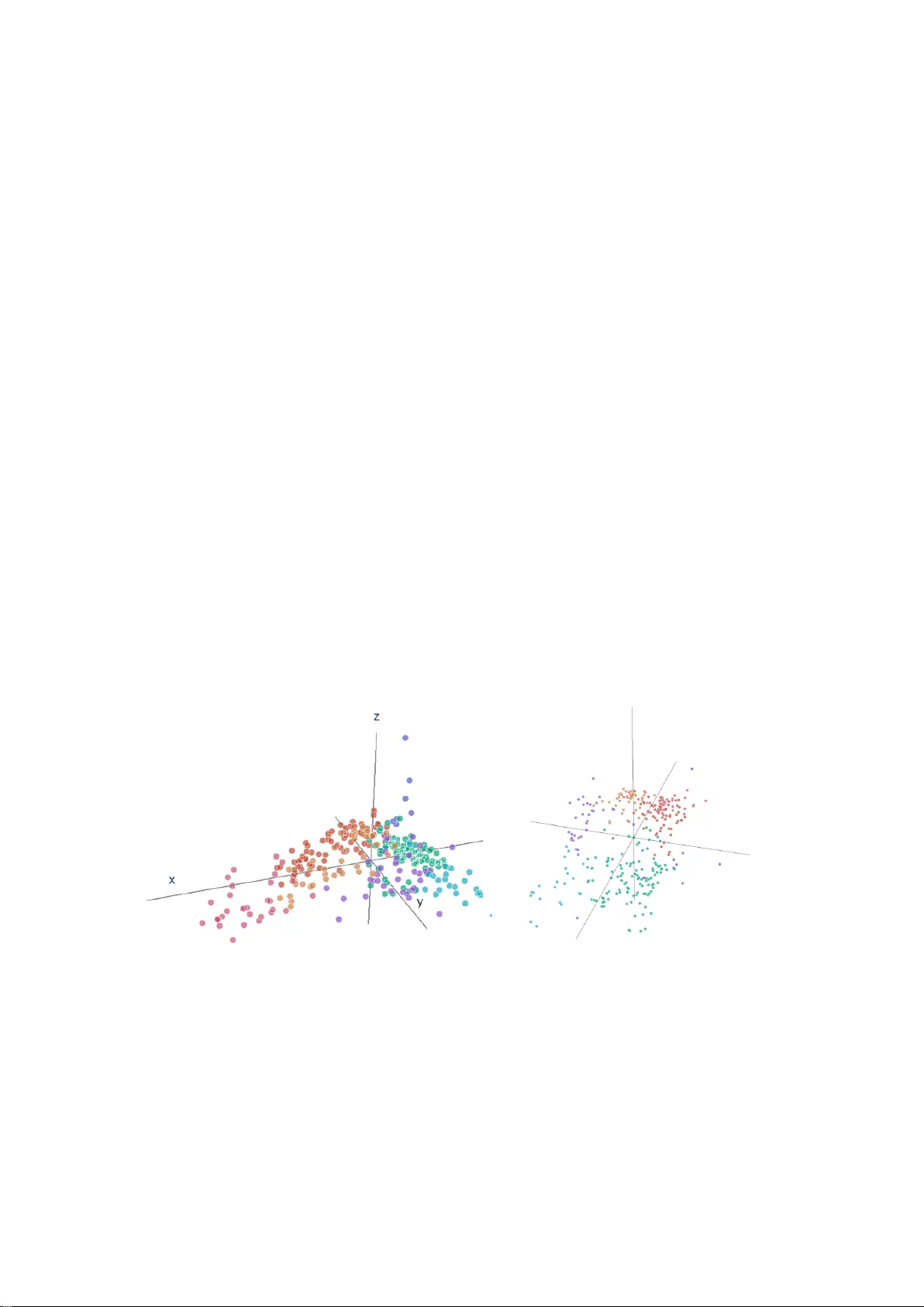
THE GEOMETR Y OF FINANCIAL INSTITUTIONS - W ASSERSTEIN CLUSTERING OF FINANCIAL D A T A L. RIESS † , ‡ , J. BACKHOFF ∗ , † , M. BEIGLBÖCK ∗ , † , J. TEMME ∗ , ‡ , AND A. WOLF ∗ , ‡ Abstract. Financial regulation requires the submission of diverse and often highly granu- lar data from ﬁnancial institutions to regulators. In turn, regulators face the challenge of condensing this data into a comprehensive map that captures the mutual similarity or dis- tance b etw een diﬀeren t institutions and identiﬁes clusters or outliers based on features like size, credit portfolio, or business mo del. Additionally , missing data due to v arying regulatory requirements for diﬀeren t t ypes of institutions, can further complicate this task. T o address these challenges, we in terpret the credit data of ﬁnancial institutions as prob- ability distributions whose respective distances can be assessed through optimal transport theory . Speciﬁcally , w e prop ose a varian t of Lloyd’s algorithm that applies to probabilit y distributions and uses generalized W asserstein barycen ters to construct a metric space. Our approach provides a solution for the mapping of the banking landscap e, enabling regulators to identify clusters of ﬁnancial institutions and assess their relativ e similarit y or distance. 1. Introduction The main contribution of this article is an algorithm that takes sev eral (discrete) probability distributions in a high-dimensional space and clusters them, representing each cluster as a p oint in a metric space. In this space, the distance betw een points reﬂects ho w diﬀeren t the underlying distributions are. A key feature of the algorithm is its abilit y to handle missing data — ev en when entire co ordinates are missing systematically from some distributions. Our original motiv ation to devise this type of algorithm stems from a challenge faced by regu- lators of the ﬁnancial industry . Data that are deliv ered from ﬁnancial institutions to the regulator consist of v arious diﬀerent formats, from highly aggregate data such as the total volume of the balance sheet, do wn to very granular data ab out individual credits describ ed by characteristics suc h as volume, interest rate, etc. T wo individual credits might then b e considered as similar if those c haracteristics take similar numerical v alues, i.e. ha v e small Euclidean distance when view ed as vectors in R d . T o build a distance b et ween ﬁnancial institutions, one can view these institutions as probability distributions on the space of p ossible credits (see Section 7.2 b elow) and determine the resp ective distance as a W asserstein distance. One can then interpret the landscap e of all ﬁnancial institutions as an ensemble of p oints in the W asserstein space, suscepti- ble to familiar metho ds of clustering, outlier detection, etc. A particular challenge which renders the problem more complicated is the “missingness of data” . Data delivered b y institutions may ha ve missing v alues. More crucially , data may b e missing systematically , as diﬀeren t institutions are required to deliver diﬀeren t data at v arying levels of detail and granularit y . Date : July 8, 2025. This research was funded in whole or in part by the A ustrian Science F und (FWF) under grants 10.55776/P36835, P35197, and Y782, and the Oesterreic hische Nationalbank (OeNB) through project EA TE II. F or op en access purp oses, the author has applied a CC BY public copyright license to any author accepted manuscript version arising from this submission. ∗ Authors listed in alphab etical order † Universit y of Vienna ‡ Oesterreichisc he Nationalbank . 1 2 L. RIESS, J. BACKHOFF, M. BEIGLBÖCK, J. TEMME, AND A. WOLF The algorithm w e prop ose as a ramiﬁcation simultaneously clusters probability measures with missing data and represents them as elements of a metric space. The principal structure follows the idea of Lloyd’s algorithm for k -means clustering and combines it with the concept of gener- alized W asserstein barycen ters, recently introduced by Delon, Gozlan and Saint-Dizier [10]. A classical approach to dealing with missing data would b e (e.g.) to impute from weigh ted nearest neigh b ors. Ho w ever, such a t yp e of imputation systematically skews results since probability distributions with less rep orted data tend to app ear closer to other p oin ts which the imputation pro cedure is attempting to mimic. This t yp e of bias may b e undesirable, e.g. when one is try- ing to identify distributions that are “atypical”, where “at ypical” could sp eciﬁcally refer to the manner in which data are missing. W e devise a particular wa y of soft imputation which accoun ts for a random element in ﬁlling up missing v alues, and in particular av oids the ab o ve mentioned bias. It will b e technically conv enient to formulate the algorithm in a more general form in Section 3. That is, we cluster and p erform soft imputation for p oints in an arbitrary metric space rather than a W asserstein space of probability measures. This allows us to simplify the presen tation and has the additional b eneﬁt that we obtain a version of classical Euclidean k -means clustering with missing data. This general persp ective allo ws us in Section 7.1 to compare our metho d to existing solutions for reconstructing the metric arrangement of Euclidean points. A dditionally , further sim ulation exp eriments can b e found in the Supplementary Material, and our metho d is compared to others when view ed solely as a clustering method. In particular, it is compared to k -p o d [7], another metho d that tackles the same problem in the Euclidean case, i.e. (11), meaning the clustering problem without imputing a priori. Notably , our clustering algorithm outp erforms k -p o d consistently . As for the imp ortant case of probabilit y distributions with miss- ing data our con tribution is detailed in Section 5 and complemented exp erimentally in Sections 7.2 and 7.3 with results using actual (anonymized) loan data rep orted by ﬁnancial institutions to Oesterreichisc he Nationalbank, the central bank of Austria. Figure 1. 3-d visualization of the A ustrian Banking Landscap e from tw o dif- feren t persp ectives. In teractive plot: https://lorenzriess.github.io/TGOFI_landscape.html Related Literature. Clustering distributions using W asserstein distances has b een explored in v arious works including [23, 36, 34, 17, 14]. This approach has also b een applied in ﬁnancial con texts, suc h as in [15], for the clustering of market regimes. In [29], Staib et al. prop osed The Geometry of Financial Institutions - W asserstein Clustering of Financial Data 3 W asserstein k -means++ as well as an initialization strategy , generalizing the classical k -means++ algorithm, cf. [4]. How ever, to the b est of our kno wledge, clustering distributions with missing co ordinates has not been in vestigated b efore. T o address this problem, w e rely hea vily on the concept of the generalized W asserstein barycen ter, in tro duced b y Delon, Gozlan, and Sain t- Dizier in [10], which extends the classical W asserstein barycen ter of Agueh and Carlier [1]. In the Euclidean case, w e are a ware of one method for the k -means problem with missing v alues whic h do es not impute p oints b eforehand. This metho d is called k -p o d and was introduced b y Chi et.al. in [7]. F or computational asp ects related to optimal transp ort and regularized W asserstein distance, we refer to the work of Cuturi [8] and the b ook [25] b y Cuturi and P eyré. A dditionally , w e use the POT package (Python package for optimal transp ort, see [11]) extensively for implementation purp oses. 2. k -means Clustering in Metric Sp aces: A Summar y Let x 1 , . . . , x N b e giv en p oin ts in a ﬁxed metric space ( X , d ) . The metric k -means problem is concerned with assigning the p oints to k clusters. The clusters hereby are gov erned by k barycen ters, i.e. an appropriate notion of a verage of the p oints in the corresp onding cluster. k -means was ﬁrst introduced b y MacQueen in [21]. The problem can b e formalized as min c j ∈X a ∈ [ k ] N N X i =1 d ( x i , c a i ) 2 , (KM) where we use the notation [ n ] := { 1 , . . . , n } , n ∈ N . In this form ulation a denotes a vector of assignmen ts, i.e. a i indicates the cluster membership of data p oint x i . The p oints c 1 , . . . , c k serv e as cluster barycen ters. F urthermore, a notion of barycenter, t ypically a function of some of the data p oints, is needed. Then, problem (KM) can b e tackled by the well-established Lloyd algorithm, cf. [20]. F ollowing an initialization phase, tw o steps are iterated: i) assignmen t step: giv en barycen ters c j ∈ X , for each i ∈ [ N ] pick a i ∈ argmin j ∈ [ k ] d ( x i , c j ) , (1) ii) barycen ter step: giv en assignmen t a , up date the barycenters, i.e. for eac h j ∈ [ k ] pic k c j ∈ barycenter ( { x i : a i = j } ) . (2) Let us give tw o examples with particular choices of data space X , metric d , and barycenter op eration, which will b e of interest in the sequel: Example 2.1. Let X = R d and d ( x, y ) = ∥ x − y ∥ 2 , the Euclidean space and distance. Then (KM) simpliﬁes to the classical k -means problem in Euclidean space, min c j ∈ R d a ∈ [ k ] N N X i =1 ∥ x i − c a i ∥ 2 2 . The barycenter function is the Euclidean mean/av erage. Example 2.2 (W asserstein k -means) . Here X = P 2 ( R d ) , the space of probability measures on R d with ﬁnite second moments, and d is taken to b e the W asserstein distance W 2 (recalled in 4 L. RIESS, J. BACKHOFF, M. BEIGLBÖCK, J. TEMME, AND A. WOLF (12) b elow). W e will henceforth write µ i = x i for i ∈ [ N ] . Then (KM) turns in to min ν j ∈P 2 ( R d ) a ∈ [ k ] N N X i =1 W 2 2 ( µ i , ν a i ) . As barycenter one takes the W asserstein barycen ter, i.e. the barycenter up dating step (2) reads ν j ∈ argmin ν ∈P 2 ( R d ) X i : a i = j W 2 2 ( µ i , ν ) . (3) Subsequen tly , w e wan t to generalize the previous examples, in particular Example 2.2, to the case in which certain co ordinates/marginals are missing for some observ ations, for an illustration see Figure 2 in Section 5. When applying Lloyd’s algorithm to a sp eciﬁc setup, one needs to sp ecify a distance function and a notion of barycen ter. In the case of a metric space it is natural to take a F réc het mean for the barycenter op eration, see [12]. In the case of missing co ordinates, ho wev er, the data do es not come from one metric space but from sev eral diﬀeren t spaces, and hence sev eral distances need to b e considered sim ultaneously . In particular, it is also necessary to consider a generalized notion of barycen ter. W e will introduce an approach to this challenge in the next section and discuss our sp eciﬁc examples in more detail in Example 3.2 and Section 5, resp ectively . 3. Clustering Projected Elements of Metric Sp aces Supp ose we are working in a metric space ( X , d ) and hav e p oints x 1 , . . . , x N ∈ X that we w an t to assign to k clusters. Ho wev er, what we actually observe are the points ˜ x i := φ i ( x i ) , where φ i : X → X i is a kno wn map into another metric space X i . F or instance, in the case X = R d the functions φ i migh t be pro jections on to subspaces. Ha ving observed ˜ x i ∈ X i deﬁne for y ∈ X d i ( ˜ x i , y ) := d ( φ − 1 i ( ˜ x i ) , y ) := inf x ∈X : φ i ( x )= ˜ x i d ( x, y ) , whic h serv es as a type of dissimilarity measure of a p oin t y ∈ X in the “full” metric space to the observ ed point ˜ x i . 3.1. Problem and Algorithm. Based on these notations, we introduce the problem min c j ∈X a ∈ [ k ] N N X i =1 d i ( ˜ x i , c a i ) 2 . (4) I.e. we wan t to ﬁnd optimal cluster barycen ters c 1 , . . . , c k ∈ X , as well as a vector a that optimally assigns each observed p oin t to a cluster. It is imp ortan t to note that we are lo oking for cluster barycen ters in the “full” space X . This ensures that w e are b e able to compare them to each observ ed point ˜ x i using d i ( ˜ x i , · ) . W e prop ose tackling (4) using the following tw o steps which are iterated in a Lloyd algorithm fashion after initializing the barycen ters: i) assignmen t step: giv en barycen ters c j ∈ X , set a i ∈ argmin j ∈ [ k ] d i ( ˜ x i , c j ) , (5) ii) barycen ter step: giv en assignmen t a , up date the barycenters, i.e. for eac h j ∈ [ k ] , set c j ∈ argmin y ∈X X i : a i = j d i ( ˜ x i , y ) 2 . (6) The Geometry of Financial Institutions - W asserstein Clustering of Financial Data 5 Let us note that step ii) do es not necessarily admit minimizers. How ever, in our tw o applica- tions – NA k -means (cf. Example 3.2) and NA W asserstein k -means (cf. Section 5) – minimizers alw ays exist. A more precise discussion of this tec hnical p oin t is given in App endix A. W e use the abbreviation “NA” for “Not A v ailable” . Th us, NA k -means and NA W asserstein k -means refer to the resp ective algorithms of Examples 2.1 and 2.2 adapted to handle missing co ordinates. Concerning initialization, w e (slightly) adapt the widely used k -means++ initialization algo- rithm introduced in [4]. In its original form, the initial cluster barycenters are selected from the observ ed p oints themselves. The algorithm b egins by choosing the ﬁrst barycenter uniformly at random from the observed p oints and then rep eatedly choosing p oints at random with probability prop ortional to their squared distance from the already chosen barycenters until k barycenters are c hosen. This approac h is not directly applicable to our setting b ecause not all p oin ts are fully observ ed, and thus not all pairwise distances can b e computed. Therefore we apply the k -means++ initialization algorithm to the subset of fully observed p oints only , i.e. those p oints x i with φ i = Id X . 3.2. Using Clustering for Imputation. After clustering w e obtain a v ector of assignments a and barycenters c 1 , . . . , c k . W e can use these to impute the not fully observed p oin ts. F or this sak e deﬁne I f := { i : φ i = Id X } , I m := [ N ] \ I f , (7) i.e. respectively the set of indices of points b eing observ ed in X (i.e. fully observ ed data) and the set of indices of p oints that are only observ ed after some non-trivial map (i.e. with missing data). The ﬁnal clusters are deﬁned b y letting for j ∈ [ k ] C j := { i ∈ [ N ] : a i = j } . W e wan t to use the clusters to ﬁnd, for a p oin t ˜ x i with i ∈ I m , a probabilit y measure on X , i.e. an element of P ( X ) , whic h attempts to concentrate around the true (unobserv ed) p oint x i . W e deﬁne for i ∈ I m the set of indices w e use for ﬁlling up the missing information of ˜ x i , as J i := I f ∩ C a i . This says that w e wan t to use the “full” p oints in the same cluster as ˜ x i in order to comp ensate the incomplete information that we hav e ab out ˜ x i . It can of course happen that J i = ∅ . In this case we use the corresponding cluster barycen ter c a i to complement the information about ˜ x i . In the following we assume J i  = ∅ . T aking now some x ℓ with ℓ ∈ J i w e set y i ℓ ∈ argmin x ∈X φ i ( x )= ˜ x i d ( x, x ℓ ) , (8) whic h will b e one p oten tial c hoice of “ﬁlling up” . W e introduce the shorthand D i ℓ := d ( y i ℓ , x ℓ ) = d i ( ˜ x i , x ℓ ) . In order to determine the w eights of a probability measure, we set p i ℓ := f ( D i ℓ ) with f : [0 , ∞ ) → [ 0 , ∞ ) b eing some p ositive decreasing function ﬁxed in adv ance, e.g. f ( x ) := exp( − x 2 ) . This wa y p i ℓ ≥ 0 and also P ℓ ∈ J i p i ℓ = 1 after p ossibly renormalizing the weigh ts by a p ositive constan t. Having obtained the w eights, we deﬁne the probability measure which should represen t a r andomly r e c onstructe d x i as θ i := X ℓ ∈ J i p i ℓ δ y i ℓ . (9) T o also em b ed the fully observed p oin ts, for i ∈ I f w e set θ i := δ x i , that is, the Dirac delta concen trated on x i . F or i ∈ I m with J i = ∅ , we use the corresp onding cluster barycenter c a i and set θ i to b e the Dirac delta concen trated on some minimizer of d ( φ − 1 i ( ˜ x i ) , c a i ) . Th us, we embed all observed p oints ˜ x 1 , . . . , ˜ x N in the same space P ( X ) . In other words, w e identify the p ossibly unobserv ed point x i with a probability measure θ i . 6 L. RIESS, J. BACKHOFF, M. BEIGLBÖCK, J. TEMME, AND A. WOLF In order to compare the hitherto constructed probability measures, as we will need to do in Section 7, we deﬁne a (generalized) metric ρ on P ( X ) . Readers primarily interested in clustering and imputation ma y skip this construction. The (generalized) metric ρ is deﬁned via the cost induced by the pr o duct or indep endent c oupling . That is, for µ, ν ∈ P ( X ) we set ρ ( µ, ν ) := 0 if µ = ν and otherwise ρ ( µ, ν ) := Z X Z X d ( x, x ′ ) µ (d x ) ν (d x ′ ) . (10) F or completeness w e provide a short lemma pro ving that ρ is indeed a (generalized) metric. Lemma 3.1. L et ( X , d ) b e a metric sp ac e and deﬁne on P ( X ) the map ρ : P ( X ) × P ( X ) → [0 , ∞ ] by ρ ( µ, ν ) := ( R X ×X d ( x, x ′ ) ( µ ⊗ ν )(d x, d x ′ ) , if µ  = ν 0 , if µ = ν. Then, ρ is a gener alize d metric on P ( X ) . Pr o of. Symmetry of the generalized metric is clear due to the symmetry of the underlying dis- tance d . Concerning the triangle inequality tak e µ, ν, θ ∈ P ( X ) which we assume to b e diﬀerent from each other (otherwise there is nothing to prov e). F urthermore, tak e three independent random v ariables X ∼ µ, Y ∼ ν , Z ∼ θ . Then, ρ ( µ, θ ) = Z X ×X d ( x, x ′ ) ( µ ⊗ θ )(d x, d x ′ ) = E [ d ( X , Z )] ≤ E [ d ( X, Y ) + d ( Y , Z )] = ρ ( µ, ν ) + ρ ( ν, θ ) , whic h prov es the triangle inequality for ρ . Concerning deﬁniteness, if µ = ν , we hav e ρ ( µ, ν ) = 0 b y deﬁnition. Supp ose now that Z X ×X d ( x, x ′ ) ( µ ⊗ ν )(d x, d x ′ ) = 0 . This implies d ( x, x ′ ) = 0 for µ ⊗ ν -almost all ( x, x ′ ) . Since d is a metric, w e ha ve x = x ′ , µ ⊗ ν -almost surely . Thus, µ = δ x = ν for some x ∈ X . □ Using a W asserstein distance or a similar notion of distance in (10), imputed p oin ts w ould b e biased to b e closer than “fully” observed p oints. The metric ρ is designed to av oid this type of bias. Indeed, our choice in (10) formalises the idea that missing v alues are not imputed in a deterministic sense but in a r andom or soft fashion, as indicated in the introduction. The distance b et ween tw o randomly imputed v alues is then estimated as an indep endent av erage of distances, follo wing the rationale that the imputation for one p oint do es not inform the imputation for a diﬀeren t point. Example 3.2 (NA k -means) . Corresp onding to classical k -means, i.e. Example 2.1, consider X = R d . Let φ i = P i : R d → R d i b e pro jections onto some of the co ordinates. Then, ˜ x i = P i ( x i ) and (4) b ecomes min c j ∈ R d a ∈ [ k ] N N X i =1 ∥ ˜ x i − P i ( c a i ) ∥ 2 2 . (11) The Geometry of Financial Institutions - W asserstein Clustering of Financial Data 7 The cluster assignment iteration step assigns eac h p oint to the cluster whose barycenter is closest, considering only the known co ordinates. The barycenter up dating step is solved by  X i : a i = j P T i P i  − 1 X i : a i = j P T i P i ( x i ) , whic h, in each co ordinate, corresp onds to the av erage of all the p oin ts in the cluster for which that co ordinate is av ailable. W e detail in Section 5 how to deal with the case where the inv erse do es not exit. By imputing missing v alues as described ab ov e, w e obtain measures in P 2 ( R d ) , of whic h we can then calculate pairwise distances using the metric ρ , deﬁned in (10). Exp eriments using this metho d ma y be found in Section 7.1. It is worth noting that [7] considers the same loss function, i.e. (11), but proposes a diﬀerent algorithm for clustering Euclidean p oin ts with missing v alues, known as k -p o d. In the Supple- men tary Material a comparison to their algorithm can b e found when w e view our metho d solely as clustering algorithm. Notably , our proposed metho d, NA k -means, consistently outp erforms k -po d. Before discussing our second example in Section 5, which generalizes Example 2.2, we ﬁrst recall the necessary notions from optimal transp ort theory . 4. W asserstein Dist ance and Generalized W asserstein Bar ycenter: a Summar y Optimal T ransp ort and W asserstein Distance. Let µ, ν be probability measures on Polish spaces X , Y resp ectiv ely . F or a measurable map T : X → Y we use # to denote the push-forward op erator of measures (image measure), i.e. for a measurable set B ⊂ Y , we put T # µ ( B ) := µ ( T − 1 ( B )) . Denote by Π( µ, ν ) := { π ∈ P ( X × Y ) : pro j X # π = µ, pro j Y # π = ν } the set of couplings of µ and ν , i.e. the set of all measures on the pro duct space having µ and ν as marginals. The Kantoro vich problem for a cost function c : X × Y → R + , introduced in [18], is inf π ∈ Π( µ,ν ) Z X × Y c ( x, y ) π (d x, d y ) . (KP) W e sp ecialize to the case X = Y = R d and c ( x, y ) = ∥ x − y ∥ p p for p ∈ [ 1 , ∞ ) . The W asserstein distance W p on the space P p ( R d ) of probability measures with ﬁnite p -momen t is then deﬁned via W p ( µ, ν ) p := inf π ∈ Π( µ,ν ) Z R d × R d ∥ x − y ∥ p p π (d x, d y ) . (12) W asserstein Barycen ter. A notion of av eraging probability measures that has recently re- ceiv ed signiﬁcan t attention is the concept of W asserstein barycenters, introduced by Agueh and Carlier [1]. A W asserstein barycenter of µ 1 , . . . , µ n ∈ P 2 ( R d ) with w eights λ 1 , . . . , λ n ≥ 0 sum- ming to 1 , is a solution of inf ν ∈P 2 ( R d ) n X i =1 λ i W 2 2 ( µ i , ν ) . Since we wan t to generalize the algorithm in tro duced in Sections 2-3 to the setting of probability measures, we require a v ariant of the W asserstein barycenter that is still applicable when only some co ordinates of the measures are known. A suitable concept, the gener alize d W asserstein b aryc enter , was in tro duced b y Julien, Gozlan and Saint-Dizier in [10]. T o formally deﬁne it, let probabilit y measures µ 1 , . . . , µ n ∈ P 2 ( R d ) b e giv en along with linear maps P i : R d → R d i . In 8 L. RIESS, J. BACKHOFF, M. BEIGLBÖCK, J. TEMME, AND A. WOLF our intended applications, these maps corresp ond to pro jections onto some of the co ordinates. A generalized W asserstein barycen ter of the push-forw arded measures P 1 # µ 1 , . . . , P n # µ n with asso ciated weigh ts λ 1 , . . . , λ n ≥ 0 summing to 1 , is a solution of inf ν ∈P 2 ( R d ) n X i =1 λ i W 2 2 ( P i # µ i , P i # ν ) . (13) T o solve the problem, it is useful to reform ulate it as a classical W asserstein barycenter problem. By asso ciating each pro jection P i with a matrix P i ∈ R d i × d , w e deﬁne A := P n i =1 λ i P T i P i and assume in the follo wing that A is inv ertible. Next, we set ¯ µ i := ( A − 1 / 2 P T i ) # µ i ∈ P 2 ( R d ) for i ∈ [ n ] , and consider the classical W asserstein barycenter problem inf ¯ ν ∈P 2 ( R d ) n X i =1 λ i W 2 2 ( ¯ µ i , ¯ ν ) . (14) Then, ν is a solution to (13) if and only if ¯ µ = A 1 / 2 # ν is a solution to (14), see Prop osition 3.1 in [10]. Regarding computational asp ects, especially in the discrete case, eﬃcien t algorithms for computing W asserstein barycenters ha ve already b een developed; see e.g. [9], as well as [37], and are implemented in the Python pac kage POT (see [11]). 5. NA W ASSERSTEIN k -MEANS Algorithm Description. W e can now discuss the case of X = P 2 ( R d ) in detail, as w e hav e established the tw o necessary op erations — the W asserstein distance and the generalized W asser- stein barycenter — for an algorithm as describ ed in Section 3. Supp ose we w an t to cluster probabilit y measures µ 1 , . . . , µ N ∈ P 2 ( R d ) in to k clusters but w e only observe their push-forw ards P i # µ i ∈ P 2 ( R d i ) under pro jections P i : R d → R d i for i ∈ [ N ] . Th us, in the language of Section 3, w e hav e φ i ( · ) := P i # ( · ) , and ˜ x i = P i # µ i =: ˜ µ i . Problem (4) then reads as inf ν j ∈P 2 ( R d ) a ∈ [ k ] N N X i =1 W 2 2 ( ˜ µ i , P i # ν a i ) . W e can tac kle this problem by the iterations suggested in Section 3.1, which read as i) up date cluster assignments given barycen ters ν j , i.e. for each i ∈ [ N ] set a i ∈ argmin j ∈ [ k ] W 2 ( ˜ µ i , P i # ν j ) , (15) ii) up date cluster barycenters given an assignment a , i.e. for eac h j ∈ [ k ] set ν j ∈ argmin ν ∈P 2 ( R d ) X i : a i = j W 2 2 ( ˜ µ i , P i # ν ) . Again, we aim to ﬁnd an optimal assignmen t v ector a that assigns each measure to one of the k clusters, as w ell as optimal barycen ters, sp eciﬁcally generalized W asserstein barycen ters, ν 1 , . . . , ν k . Note that once again, we are lo oking for barycen ters in the full space P 2 ( R d ) , i.e. ha ving all co ordinates. It ma y happ en that a cluster consists entirely of measures missing the same co ordinate, i.e. for some j ∈ [ k ] , w e hav e \ i : a i = j k er P i  = { 0 } . T o a void numeric al problems in such cases, one can initialize the barycenters without missing co ordinates and adapt step ii) to include the previous barycenter with a small weigh t. This The Geometry of Financial Institutions - W asserstein Clustering of Financial Data 9 ensures that all subsequent barycen ters hav e no missing co ordinates. Speciﬁcally , assume that at iteration t the barycenters are ν ( t ) j ∈ P 2 ( R d ) and a new assignment v ector a ( t +1) ∈ [ k ] N has b een computed. Given a weigh t λ ( t ) ∈ (0 , 1) , set ν ( t +1) j ∈ argmin ν ∈P 2 ( R d ) (1 − λ ( t ) ) X i : a ( t +1) i = j W 2 2 ( ˜ µ i , P i # ν ) + λ ( t ) W 2 2 ( ν ( t ) j , ν ) . (16) Exp erimen tally we ha ve observ ed that λ ( t ) := 1 ( t +1) 1 / 2 w orks w ell. Ha ving deﬁned the tw o iterativ e steps, we now present the main computational contribution of this w ork: Algorithm 1. If no prior information is av ailable, we prop ose initializing it as describ ed in Section 3.1. Algorithm 1 NA W asserstein k -means Input: N observ ed measures ˜ µ i = P i # µ i , n umber of clusters k , maximum num b er of iterations T , weigh ting schedule ( λ ( t ) ) T t =0 Result: barycenters ν j , assignments a Initialize t = 0 , ν (0) 1 , . . . , ν (0) k ∈ P 2 ( R d ) , and a (0) ∈ [ k ] N while t < T do for i = 1 to N do a ( t +1) i := argmin j ∈ [ k ] W 2 2 ( ˜ µ i , P i # ν ( t ) j ) (17) end for for j = 1 to K do c ho ose ν ( t +1) j according to (16) by including the old barycenter ν ( t ) j with weigh t λ ( t ) end for if a ( t ) == a ( t +1) then break end if t := t + 1 end while In (17) we use the en try of the old assignment v ector a ( t ) i if it is a minimizer. This leads to a simple conv ergence result. F or this sak e let L ( ν 1 , . . . , ν K , a ) := N X i =1 W 2 2 ( P i # µ i , P i # ν a i ) . (18) Theorem 5.1. Given an initialization ν (0) 1 , . . . , ν (0) k ∈ P 2 ( R d ) , a (0) ∈ [ k ] N , A lgorithm 1 strictly de cr e ases L until it terminates after ﬁnitely many steps, for any choic e of ( λ ( t ) ) t ∈ N (even for T = ∞ ). If in every iter ation e ach cluster has a me asur e with al l c o or dinates, then Algorithm 1 with λ ( t ) = 0 yields a lo c al minimum of L . Remark 5.2 (Sp eed of conv ergence) . It is kno wn that the classical Euclidean k -means algorithm can require an exp onential n um b er of iterations in the worst-case. Speciﬁcally , there exists a lo wer b ound 2 Ω( N ) ev en in t w o dimensions, see [33, 3]. Since Algorithm 1 includes k -means as a sp ecial case (sp eciﬁcally , when applied to Dirac measures, i.e. Euclidean data, without missing v alues), this worst-case b ehavior also applies to our metho d. It cannot b e w orse than exp onen tial, ho wev er, due to the trivial upper b ound k N of p ossible cluster assignmen ts. Nev ertheless, in practice, k -means typically conv erges within a mo derate n umber of iterations - often around 20 to 50 - when clustering a not-to o-large num b er of ob jects, see [13, 6]. In our exp erimen ts, w e observ ed a similar b eha vior for b oth NA W asserstein k -means and NA k - means. On a verage, the n um b er of iterations hov ered around 30 iterations without exceeding 50 . 10 L. RIESS, J. BACKHOFF, M. BEIGLBÖCK, J. TEMME, AND A. WOLF Sp eciﬁcally , in all exp erimen ts, we set the maximum num b er of iterations to 100 and this b ound w as nev er reached. Pr o of of The or em 5.1. Let us ﬁrst sho w that the loss function decreases monotonically . Using the assignment step in the ﬁrst and the barycen ter up dating step in the second inequalit y , we obtain (1 − λ ( t +1) ) L ( ν ( t ) 1 , . . . , ν ( t ) k , a ( t ) ) = (1 − λ ( t +1) ) N X i =1 W 2 2  P i # µ i , P i # ν ( t ) a ( t ) i  ( ⋆ ) ≥ (1 − λ ( t +1) ) N X i =1 W 2 2  P i # µ i , P i # ν ( t ) a ( t +1) i  = k X j =1 h (1 − λ ( t +1) ) X i : a ( t +1) i = j W 2 2 ( P i # µ i , P i # ν ( t ) j ) + λ ( t +1) W 2 2 ( ν ( t ) j , ν ( t ) j ) | {z } =0 i ≥ k X j =1 h (1 − λ ( t +1) ) X i : a ( t +1) i = j W 2 2 ( P i # µ i , P i # ν ( t +1) j ) + λ ( t +1) W 2 2 ( ν ( t ) j , ν ( t +1) j ) | {z } ≥ 0 i ≥ (1 − λ ( t +1) ) N X i =1 W 2 2  P i # µ i , P i # ν ( t +1) a ( t +1) i  = (1 − λ ( t +1) ) L ( ν ( t +1) 1 , . . . , ν ( t +1) k , a ( t +1) ) . Since 1 − λ ( t +1) > 0 , this shows the monotonicity . In inequality ( ⋆ ) , equalit y holds if and only if there is no change in the assignment step, i.e. if a ( t ) i = a ( t +1) i , ∀ i ∈ [ N ] . In this case the algorithm terminates. If there is some i ∈ [ N ] such that a ( t ) i  = a ( t +1) i , then we ha ve a strict inequality , since the assignment in Algorithm 1, cf. (17), is only up dated when L decreases due to the new assignment. Since only a ﬁnite num b er of p ossible assignments exist, due to the fact that we are cluster- ing ﬁnitely many measures in to ﬁnitely many clusters, the algorithm strictly decreases L and terminates after a ﬁnite n um b er of steps, thus concluding the pro of. □ Remark 5.3 (Con vergence in abstract metric spaces) . In the setting of abstract metric spaces, that is, Section 3.1, we can mo dify the assignmen t step as in Algorithm 1 – that is, assignments are only up dated when the loss function strictly decreases. If we further assume that barycenters alw ays exist, the con v ergence of the algorithm follows by the same arguments as in the previous pro of. A T oy Example. T o illustrate the algorithm, consider six measures on the plane, one of which misses the vertical co ordinate (indicated by vertical lines). Eac h measure consists of three supp ort p oin ts with equal weigh t. The measures are visualized by diﬀerent colors and depicted on the left of Figure 2. When clustering these measures into three clusters, the natural choice of clusters is eviden t. Applying the ab o v e algorithm indeed yields the results shown in Figure 2. T o obtain these results, we calculated free supp ort barycen ters at each step of the algorithm with a ﬁxed supp ort size of three (cf. [38, 9]). F or the blue and brown barycenters, each support p oint is precisely the a verage of the supp ort p oints of the tw o measures in that cluster. F or the pink barycen ter the situation is slightly diﬀerent. In the y coordinate it inherits the v alues from the The Geometry of Financial Institutions - W asserstein Clustering of Financial Data 11 Figure 2. (left): 6 Measures on the Plane of Whic h One Misses the V ertical Co ordinate of Its P oints. (right) Clustering of the 6 Measures In to 3 Clusters. red measure, while as in the x co ordinate the supp ort p oin ts are the av erages of the x co ordinates of a red and a rose supp ort p oin t, resp ectively . Imputation via NA W asserstein k -means. Next, we consider how the imputation proce- dure describ ed in Section 3.2 lo oks, when X = P 2 ( R d ) . Having clustered measures P i # µ i ∈ P 2 ( R d i ) , i ∈ [ N ] , we obtain generalized W asserstein barycenters ν 1 , . . . , ν k ∈ P 2 ( R d ) and a vec- tor of assignments a ∈ [ k ] N . F or measures that are not fully observ ed, i.e. for i ∈ I m (see (7) for the deﬁnition), we will use the fully observ ed measures in the same cluster, i.e. µ ℓ with ℓ ∈ J i , to impute P i # µ i in a randomized fashion. Therefore, we ha v e to interpret (8) in the current setting. Sp eciﬁcally , for µ ℓ with ℓ ∈ J i w e need to ﬁnd η i ℓ ∈ argmin η ∈P 2 ( R p ) P i # η = P i # µ i W 2 2 ( η , µ ℓ ) . (19) T o obtain suc h η i ℓ w e will apply the follo wing lemma. Lemma 5.4. L et µ 1 ∈ P 2 ( R k ) , ν ∈ P 2 ( R d ) with d > k . Denote by ν 1 the pr oje ction on the ﬁrst k c o or dinates and by π ∗ 1 ∈ Π( µ 1 , ν 1 ) the optimal tr ansp ort c oupling b etwe en µ 1 and ν 1 . Then, the me asur e η ∗ (d x 1 , d x 2 ) := Z Y 1 ν y 1 (d x 2 ) π ∗ 1 (d x 1 , d y 1 ) , (20) solves min η ∈P 2 ( R d ) η 1 = µ 1 W 2 2 ( η , ν ) = W 2 2 ( µ 1 , ν 1 ) . (21) Pr o of. Let us ﬁrst note that for any η ∈ P 2 ( R d ) with η 1 = µ 1 there is the trivial b ound W 2 2 ( η , ν ) ≥ W 2 2 ( η 1 , ν 1 ) = W 2 2 ( µ 1 , ν 1 ) . (22) W e will show that η ∗ , as deﬁned in (20) ac hieves this low er b ound, which will imply its optimality . In order to do this, we deﬁne a coupling π ∈ Π( η ∗ , ν ) ha ving those costs. In the following w e split a p oint z ∈ R d lik e z = ( z 1 , z 2 ) ∈ R k × R d − k and use the notations X 1 , X 2 , Y 1 , Y 2 to emphasize o ver whic h space we are integrating, even though X 1 = Y 1 = R k and X 2 = Y 2 = R d − k . Let us deﬁne π by π (d x 1 , d y 1 , d x 2 , d y 2 ) := π ∗ 1 (d x 1 , d y 1 ) ν y 1 (d y 2 ) δ y 2 (d x 2 ) . (23) 12 L. RIESS, J. BACKHOFF, M. BEIGLBÖCK, J. TEMME, AND A. WOLF T o see that this is actually a coupling of ( η ∗ , ν ) , note that for the second marginal, we ha ve Z X 1 × X 2 π ∗ 1 (d x 1 , d y 1 ) ν y 1 (d y 2 ) δ y 2 (d x 2 ) = Z X 1 Z X 2 δ y 2 (d x 2 ) π ∗ 1 (d x 1 , d y 1 ) ν y 1 (d y 2 ) = Z X 1 π ∗ 1 (d x 1 , d y 1 ) ν y 1 (d y 2 ) = ν 1 (d y 1 ) ν y 1 (d y 2 ) = ν (d y 1 , d y 2 ) . F or the ﬁrst marginal, we hav e Z Y 1 × Y 2 π ∗ 1 (d x 1 , d y 1 ) ν y 1 (d y 2 ) δ y 2 (d x 2 ) = Z Y 1 Z Y 2 δ y 2 (d x 2 ) ν y 1 (d y 2 ) π ∗ 1 (d x 1 , d y 1 ) = Z Y 1 ν y 1 (d x 2 ) π ∗ 1 (d x 1 , d y 1 ) = η ∗ (d x 1 , d x 2 ) . Next, let us calculate the coupling’s cost, Z X × Y | x − y | 2 π (d x, d y ) = Z X 1 × Y 1 | x 1 − y 1 | 2 π ∗ 1 (d x 1 , d y 1 ) + Z X × Y | x 2 − y 2 | 2 π (d x, d y ) = W 2 2 ( µ 1 , ν 1 ) + Z X × Y | x 2 − y 2 | 2 π (d x, d y ) , and note for the second term, Z X × Y | x 2 − y 2 | 2 π (d x, d y ) = Z X 1 × Y 1 Z Y 2 Z X 2 | x 2 − y 2 | 2 δ y 2 (d x 2 ) ν y 1 (d y 2 ) π ∗ 1 (d x 1 , d y 1 ) = 0 . Therefore, W 2 ( η ∗ , ν ) = W 2 ( µ 1 , ν 1 ) , showing that η ∗ solv es (21). □ Remark 5.5. If π ∗ 1 in Lemma 5.4 is of Monge-type, i.e. if there is a measurable map T 1 : R k → R k suc h that π ∗ 1 = (id R k , T 1 ) # µ 1 , then (20) simpliﬁes to η ∗ (d x 1 , d x 2 ) = µ 1 (d x 1 ) ν T 1 ( x 1 ) (d x 2 ) . (24) Lemma 5.4 describ es the form of η i ℓ in (19). T o apply it, let π i ℓ ∈ Π( P i # µ i , P i # µ ℓ ) b e the optimal coupling b et ween P i # µ i and P i # µ ℓ . A dditionally , let I i ⊂ [ d ] denote the indices of the pro jection P i , i.e. P i ( x 1 , . . . , x d ) = ( x j ) j ∈I i , and for the remaining indices deﬁne I C i := [ d ] \ I i . A solution to (19) then is η i ℓ (d x 1 , . . . , d x d ) := Z R |I C i | µ ℓ ( y j ) j ∈I i ((d x j ) j ∈I C i ) π i ℓ ((d x j , d y j ) j ∈I i ) . (25) Ha ving this, we can translate (9) to the current setting by using η i ℓ with ℓ ∈ J i , and deﬁne P i := X ℓ ∈ J i p i ℓ δ η i ℓ (26) to obtain a measure P i ∈ P 2 ( P 2 ( R d )) , i.e. a random measure. F or fully observed measures, i.e. i ∈ I f w e set P i := δ µ i . F or i ∈ I m and | J i | > 1 we suggest the weigh ts p i ℓ ∝ exp  − λ 2 σ 2 i W 2 2 ( P i # µ i , P i # µ ℓ )  , ℓ ∈ J i . This reﬂects the idea that measures whic h are closer to the to b e imputed measure in the known co ordinates should receive more w eight. Here, λ > 0 is a tuning parameter that controls this The Geometry of Financial Institutions - W asserstein Clustering of Financial Data 13 w eighting and the v ariance σ 2 i is used to standardize the distances, i.e. σ 2 i := 1 | J i | − 1 X ℓ ∈ J i W 2 2 ( P i # µ i , P i # µ ℓ ) . If | J i | = 1 it is clear what to do, as there is only one measure av ailable for imputation and for | J i | = 0 we use the barycenter ν a i to impute P i # µ i . After imputation we obtain random measures P 1 , . . . , P N ∈ P 2 ( P 2 ( R d )) . T o calculate their pairwise distances, we use the metric ρ deﬁned in (10). That is, for P , Q ∈ P 2 ( P 2 ( R d )) , ρ ( P , Q ) = 0 , if P = Q , and for P  = Q ρ ( P , Q ) = Z P 2 ( R d ) Z P 2 ( R d ) W 2 ( µ, ν ) P (d µ ) Q (d ν ) . (27) 6. Ev alua tion Method Our main motiv ation for NA W asserstein k -means was to develop a metho d for clustering and reconstructing measures that may hav e missing co ordinates. T o the b est of our knowledge, this is the ﬁrst metho d to address this problem, so we cannot compare it to existing metho ds. In this short section w e prop ose an abstract metho dology for ev aluating the quality of a reconstruction metho d in the setting of metric (measure) spaces, based on the concept of Gromov-W asserstein distance. As just explained this ev aluation metho dology will not b e applied directly to our main problem of interest, since there is no alternative metho d to compare to. How ever, we will apply it to a related problem in Section 7.1, where the data consists of Euclidean p oints rather than measures. F or the Euclidean case we can compare NA k -means, a sp ecial case of NA W asserstein k -means, to existing alternative metho ds. Supp ose there are elements x 1 , . . . , x N in a metric space ( X , d X ) , which we collect in the set X := { x 1 , . . . , x N } . The data we observe are these p oints but only via the maps φ i : X → X i deﬁned in Section 3, i.e. we observ e ˜ x i = φ i ( x i ) . The observ ed p oin ts are collected in ( ˜ x 1 , . . . , ˜ x N ) ∈ X N A , where we deﬁne X N A := X 1 × · · · × X N . This can b e summarized by saying that w e only observe the v alues of ( x 1 , . . . , x N ) under the map h : X N → X N A , in particular h i ( x 1 , . . . , x N ) = φ i ( x i ) = ˜ x i . The goal is to reconstruct the metric structure of X = { x 1 , . . . , x N } , whic h is describ ed b y their resp ectiv e pairwise distances, as accurately as p ossible. This means that w e w an t to ﬁnd a go o d metric space ( Y , d Y ) and a reconstruction map R : X N A → Y N . The reconstructed p oint corresp onding to x i then is R i ( ˜ x 1 , . . . , ˜ x N ) = y i . Before establishing a wa y of comparing the reconstructed p oin ts R (( ˜ x 1 , . . . , ˜ x N )) = ( y 1 , . . . , y N ) to the original p oints X , w e wan t to consider another piece of information, namely that some observ ations of X might b e more imp ortan t for us than others. This is motiv ated by our main in tended application of reconstructing a banking landscap e, in which a bank’s importance may b e linked to attributes such as its size, measured, for example, by its total assets. This follows the rationale that for a regulator it ma y b e more imp ortant to reconstruct the characteristics of a very large bank than those of a smaller bank. A simple wa y to account for this is to assign w eights prop ortional to the (or a function of ) size of the bank. F ormally , we deﬁne a probability measure µ X on X by setting µ X ( { x i } ) := p i ≥ 0 , where we assume P N i =1 p i = 1 . Naturally we deﬁne µ Y , a probability measure on Y , via µ Y ( { y i } ) = µ Y ( R i ( ˜ x 1 , . . . , ˜ x N )) := p i . Mémoli [22], and the related work of Sturm [30], in tro duced the Gr omov-W asserstein distanc e GW 2 in order to compare metric measure spaces. F or tw o metric measure spaces ( X , d X , µ ) and 14 L. RIESS, J. BACKHOFF, M. BEIGLBÖCK, J. TEMME, AND A. WOLF ( Y , d Y , ν ) , it is deﬁned as GW 2 (( X , d X , µ ) , ( Y , d Y , ν )) 2 := inf π ∈ Π( µ,ν ) Z X 2 ×Y 2 | d X ( x, x ′ ) − d Y ( y , y ′ ) | 2 π (d x, d y ) π (d x ′ , d y ′ ) . W e will use the Gromov-W asserstein distance to ev aluate a reconstruction, i.e. w e will use GW 2  ( X , d X , µ X ) , ( { R 1 ( ˜ x 1 , . . . , ˜ x N ) , . . . , R N ( ˜ x 1 , . . . , ˜ x N ) } , d Y , ν Y )  (28) as p erformance measure. Note, that in the case of reconstructing as describ ed in Section 3.2, we ha ve Y = P ( X ) . F or algorithms to compute the Gromov-W asserstein distance we refer to [22] and [26], which are implemented in Python optimal transp ort library POT (see [11]). W e will use this implemen tation in Section 7.1. The curious reader is also referred to [2, 32, 26] for some mac hine learning applications of Gromo v-W asserstein distances and related metrics. 7. Experiment al Resul ts 7.1. Reconstructing P oin ts from a Gaussian Mixture Mo del. W e start by comparing our clustering / reconstruction metho d with existing imputation metho ds in the Euclidean case, i.e. X = R d , and ev aluate the results using the Gromov-W asserstein distance, cf. (28), introduced in Section 6. W e simulate data from a Gaussian Mixture Mo del γ := k X j =1 α j N ( µ j , Σ j ) , (29) with weigh ts α 1 , . . . , α k ≥ 0 and P k j =1 α j = 1 . Additionally , to simulate the imp ortance of p oin ts, i.e. µ X ( { x i } ) from Section 6, we draw samples from a Lognormal ( µ, σ 2 ) distribution and assign each observ ation a weigh t prop ortional to its sampled v alue. In our sim ulation study we ﬁx the parameters k = 5 , d = 5 , and N = 500 , mean ing that we alwa ys sample 500 p oin ts. T o sim ulate missing v alues we employ v arious missingness structures, corresp onding to diﬀerent c hoices of the map h from Section 6. Little and R ubin [19] classify missing data mechanisms in to the following three categories: • MCAR (missing completely at random): The probability of a missing v alue do es not dep end on any observed or unobserved v alues. • MAR (missing at random): The probability of a missing v alue dep ends only on observed data, not on the missing data itself. • MNAR (missing not at random): The probabilit y of a missing v alue dep ends on the missing v alues themselves, even when accounting for observ ed data. In order to achiev e robust results w e incorporate diﬀerent combinations of all these missingness mec hanisms in our simulation study , i.e. in our deﬁnition of h from Section 6. Before describing the metho d used to create missing v alues, we ﬁrst explain how the parameters for the data-generating pro cess are chosen, i.e. α 1 , . . . , α k , µ 1 , . . . , µ k , Σ 1 , . . . , Σ k for the Gaussian Mixture Mo del, and µ, σ 2 for the lognormal distribution go verning the imp ortance of sampled p oin ts. W e set µ = 20 , σ = 1 . 5 , as these parameters (empirically) mo del the total assets of a ﬁnancial institution reasonably well. F or the Gaussian Mixture Mo del, we aim to simulate the w eights of the normal distributions, means and cov ariance matrices in a non-informative manner. Sp eciﬁcally , the weigh ts α j are sampled uniformly from the probability simplex, the means µ j ’s are sampled uniformly from the cube [ − 5 , 5] d and the cov ariance matrices Σ j ’s are drawn from a Wishart distribution with parameters ( d, Id d /d ) . Note that with this c hoice of parameters for the Wishart distribution, we ha ve E [Σ j ] = Id d . The Geometry of Financial Institutions - W asserstein Clustering of Financial Data 15 In order to create missing data, w e aim to com bine the t yp es of missingness mechanisms describ ed ab ov e. T o achiev e this, we choose weigh ts β M C AR , β M AR , β M N AR ≥ 0 with β M C AR + β M AR + β M N AR = 1 . W e then ﬁx a prop ortion p ∈ (0 , 1) which determines the total fraction of missing v alues. Given N = 500 p oints sampled indep enden tly from γ , w e compute for each dimension the pβ M N AR quan tile and pro ceed to create missing v alues as follo ws: i) MCAR : set 100 pβ M C AR % v alues missing completely at random, ii) MNAR : for eac h dimension set all v alues to missing which are b elo w the corresp onding pβ M N AR quan tile, iii) MAR : for p oin ts where the ﬁrst co ordinate is observ ed and non-negative, the probability of missing v alues in the other co ordinates is four times higher than for p oin ts where the ﬁrst co ordinate is observed and negativ e. In total, we create 100 pβ M AR % of missing v alues in the data follo wing this rule. This pro cedure deﬁnes the map h from Section 6. T o generate the results in T able 1, we set p = 0 . 15 . F or β M C AR , β M AR , and β M N AR , w e consider seven diﬀeren t combinations by applying eac h t yp e of missingness individually , in pairs, and all three types together. F or each choice of β M C AR , β M AR , β M N AR , we sample the describ ed parameters of the Gauss- ian Mixture Model 100 times. W e generate data, and compute pairwise distances b etw een data p oin ts. Then, w e create missing v alues according to h and apply diﬀerent imputation pro cedures presen ted b elo w. If missing v alues are imputed by p oints, w e compute pairwise distances b etw een the imputed p oints. If the imputation is done via measures, as abstractly deﬁned in (9), we use the distance ρ from Section 3.2 to compute pairwise distances. Finally , we calculate the cor- resp onding Gromov-W asserstein distance b etw een original pairwise distances and the imputed pairwise distances, using the corresp onding weigh ts deriv ed from the Lognormal ( µ, σ 2 ) samples, i.e. we compute (28). In our exp erimen t we lo ok at the following imputation tec hniques: • NA k -means: Our method in the case of Euclidean data, as outlined in Example 3.2. • NA k -means-m: this corresp onds to ﬁrst applying NA k -means for clustering and impu- tation. After obtaining the measures ( θ i ) N i =1 , we compute their exp ected v alues and use them as the imputed p oin ts. • Mean imputation: Each missing v alue is replaced by the mean of the corresp onding attribute. • Median imputation: Each missing v alue is replaced b y the median of the corresp onding attribute. • Multiple imputation: A metho d [28, 5] that imputes missing v alues by generating mul- tiple p ossible v alues and com bines results. • KNN: K-nearest-neighbor imputation, where each missing v alue is replaced by a weigh ted a verage of p oin ts that are close in the co ordinates which are not missing. W e choose K = 4 . • LR: Missing v alues are imputed by regressing on observed v alues and using the predicted v alues as imputations. F or all metho ds not introduced in this article, i.e. all except NA k -means and NA k -means-m, w e use the implementations from scikit-learn , [24]. In T able 1, w e rep ort the estimated Gromov W asserstein Distances along with their standard errors, based on sampling 100 times for each com bination of β M C AR , β M AR and β M N AR . W e observe that, in the case of Euclidean p oints with missing v alues, the prop osed metho d con- sisten tly outp erforms classical imputation techniques when considering the Gromov-W asserstein distance as ev aluation measure. Speciﬁcally , whether we apply NA k -me ans directly or include an additional av eraging step, i.e. NA k -me ans-m , b oth algorithms outp erform the remaining ﬁve metho ds across all considered missing data scenarios, i.e. com binations of MCAR, MAR and 16 L. RIESS, J. BACKHOFF, M. BEIGLBÖCK, J. TEMME, AND A. WOLF T able 1. Gromov W asserstein Distance for Euclidean Simulation with p = 0 . 15 . β M C AR β M AR β M N AR NA k -means. NA k -means-m mean imp. median imp. KNN multiple imp. LR 1 0 0 0.525 ± 0.016 0.549 ± 0.021 1.28 ± 0.024 1.28 ± 0.024 0.643 ± 0.014 0.724 ± 0.02 0.734 ± 0.02 0 1 0 0.517 ± 0.012 0.574 ± 0.03 1.296 ± 0.034 1.296 ± 0.034 0.619 ± 0.021 0.791 ± 0.029 0.802 ± 0.033 0 0 1 1.534 ± 0.048 1.592 ± 0.052 2.316 ± 0.053 2.316 ± 0.053 1.792 ± 0.047 1.719 ± 0.051 1.743 ± 0.053 0.5 0.5 0 0.51 ± 0.017 0.513 ± 0.016 1.286 ± 0.029 1.286 ± 0.029 0.627 ± 0.019 0.703 ± 0.019 0.709 ± 0.021 0 0.5 0.5 1.035 ± 0.036 1.12 ± 0.04 1.86 ± 0.033 1.86 ± 0.033 1.308 ± 0.034 1.306 ± 0.039 1.316 ± 0.042 0.5 0 0.5 1.012 ± 0.03 1.106 ± 0.039 1.883 ± 0.033 1.883 ± 0.033 1.347 ± 0.04 1.311 ± 0.038 1.335 ± 0.038 0.333 0.333 0.333 0.872 ± 0.035 0.918 ± 0.037 1.702 ± 0.028 1.702 ± 0.028 1.125 ± 0.028 1.126 ± 0.028 1.145 ± 0.033 MNAR. In the Supplementary Material w e use the (adjusted) Rand index [27, 16] as ev aluation metho d when treating NA k -means purely as a clustering algorithm, rather than as a metho d to reconstruct the metric structure of ob jects, i.e. as imputation metho d. There we also compare it to k -p o d which is consistently outp erformed by NA k -means (see T able 3). Moreo ver, we pro vide results for additional v alues of p , i.e. the total share of missing v alues in the observed data, to accompan y and robustify our results. 7.2. Reconstructing Financial Institutions. As describ ed in the introduction, the primary motiv ation for dev eloping NA W asserstein k -means comes from clustering ﬁnancial institutions based on gran ular loan data they are obliged to rep ort to the central bank. This problem is of particular interest to regulators, as it enables a data-driv en assessment of similarities and diﬀerences b et w een ﬁnancial institutions. If prior b eliefs ab out similarities exist, this metho d pro vides a w a y to conﬁrm or challenge them. In particular, if ﬁnancial institutions hav e already b een group ed based on prior knowledge, our approach can serve as a v alidation to ol, highlighting institutions whose cluster assignment deviates from the exp ected grouping and may therefore w arrant further inv estigation. Before presen ting an exp eriment of applying NA W asserstein k -means, note that there is another exp eriment justifying the usage of NA W asserstein k -means in Section 7.3. T o demonstrate NA W asserstein k -means in a practical example, we use real data from Oester- reic hische Nationalbank, the central bank of Austria, and analyze loan data rep orted by 321 ﬁnancial institutions in Austria. In total, our dataset consists of 129230 loans. Each loan is describ ed b y up to four attributes: interest rate, interest rate margin, probabilit y of default and par v alue. In our analysis w e apply a logarithmic transformation to par v alue and then standard- ize all four attributes across all loans. Additionally , we account for loan size by weigh ting each loan within a ﬁnancial institution prop ortionally to the logarithm of its size. Among the 321 institutions, 265 rep orted all four attributes, 45 institutions rep orted three and 11 institutions rep orted only t wo. As a result, our observed data consists of 265 probabilit y measures in P 2 ( R 4 ) , 45 probability measures in P 2 ( R 3 ) and 11 probability measures in P 2 ( R 2 ) . Ideally , the complete dataset w ould consist of 321 probability measures in P 2 ( R 4 ) but due to diﬀerences in rep ort- ing, missing v alues must b e accounted for in practice. While meaningful imputation is already c hallenging for Euclidean data, it is even more diﬃcult when dealing with measure-v alued data. Since prior imputation is not necessary for NA W asserstein k -means, we can apply it directly as describ ed in Section 5 and cluster the ﬁnancial institutions in to seven groups. After clustering, we use the imputation metho d describ ed in the same section to obtain random measures P 1 , . . . , P 321 on R 4 , cf. Equation (19). Using the generalized distance ρ on P 2 ( P 2 ( R 4 )) , deﬁned in (27), we compute pairwise distances b et ween the (imputed) ﬁnancial institutions. Once the pairwise distances are computed, it is p ossible to visualize the reconstructed ﬁnancial institutions and clustering results. T o create such a banking landscap e, dimensionality reduction techniques may b e applied to approximate pairwise distances in a low er-dimensional space. Here, w e choose Isomap (cf. [31]) o v er other methods, such as multidimensional scaling, as it is b etter suited to reco ver nonlinear manifolds. Applying Isomap to the pairwise distance matrix ( ρ ( P i , P j )) 321 i,j =1 The Geometry of Financial Institutions - W asserstein Clustering of Financial Data 17 maps the ﬁnancial institutions to R 3 while preserving the ov erall distance structure as closely as p ossible. Figure 1 presents the result of this three-dimensional representation, i.e. a banking landscape with the corresp onding clusters. Each p oint in the ﬁgure represents one of the 321 ﬁnancial institutions, and each color describ es a cluster. A regulatory analyst can now use this three- dimensional represen tation to reassess prior b eliefs about the banking landscap e or existing groupings of ﬁnancial institutions and to identify institutions of particular interest. Additionally to prior b eliefs, the visualization may help analysts to further their understanding which ﬁnan- cial institutions are similar to eac h other and also identify ﬁnancial institutions whic h behav e signiﬁcan tly diﬀerent to others with resp ect to their loan structure. Detecting p otential outliers is of particular interest. W e also note that, having imputed the measures, i.e. “reconstructed” ﬁnancial institutions, in particular having computed their pairwise distances ( ρ ( P i , P j )) 321 i,j =1 , any distance-based learning algorithm can b e applied. Sp eciﬁcally , distance-based outlier algorithms can b e used to iden tify institutions that deviate signiﬁcantly from the rest. T o conclude this exp eriment, we emphasize that clustering probabilit y measures directly using NA W asserstein k -means can yield signiﬁcantly diﬀerent results compared to clustering their aggregated data, such as their exp ectations, with metho ds like NA k -means. T o illustrate this, w e computed the exp ected v alues of the 321 probability measures considered in this section and applied NA k -means to the resulting p oints (with possibly missing v alues) in R 4 . Using the obtained cluster lab els, we then computed generalized W asserstein barycenters for these clusters. Notably , when these assignments and barycenters were used in the loss function Equation (18), the resulting v alue w as 22 . 26% higher than when clustering the probabilit y measures directly using Algorithm 1. F urthermore, comparing the lab els of the tw o clusterings using the adjusted Rand index 1 yielded a v alue of 0 . 2058 , indicating v ery p oor agreement, as a v alue of 0 would corresp ond to the exp ected agreemen t of a random assignment. This highlights the adv antage of clustering in the space of probability measures rather than relying on simple data aggregation. 7.3. Justifying NA W asserstein k -means. T o justify the use of NA W asserstein k -means, w e carry out another exp erimen t. It is similar to the one in Section 7.1, where we artiﬁcially create missing v alues, but this time using distributional data . T o the b est of our knowledge, no existing metho d can cluster probability measures that are only observed as push-forwards under pro jections. Therefore, we p erform an exp erimen t on the real loan data from the previous section, simulating missing v alues completely at random. Sp eciﬁcally , w e consider 100 ﬁnancial institutions from the previous section that rep orted all four attributes of their credits, meaning there w ere no missing v alues. F or each of these institutions we sample 100 credits to reduce the supp ort size and, consequen tly , the computational cost, as NA W asserstein k -means will b e applied m ultiple times to obtain reliable standard errors. The resulting 100 probability measures on R 4 con tain no missing v alues, allowing us to cluster them into ﬁv e groups using W asserstein k -means. The assignments from this clustering serve as the “ground truth” for this exp eriment. Next, we create missing v alues completely at random: w e choose a p ercentage p ∈ (0 , 1) and a num b er of aﬀected dimensions d m ∈ { 1 , 2 } . Then, we randomly select 100 p institutions and for each selected institution, we randomly c ho ose d m of the 4 dimensions and set them to NA. After sim ulating missing v alues in this w ay , we apply NA W asserstein k -means and compare the resulting cluster assignments to the ground truth using the adjusted Rand index. 1 1 The Rand index [27] is a similarit y measure that ev aluates the agreement b etw een tw o clusterings b y con- sidering agreement or non-agreement of all pairwise assignments. It takes the v alue 1 for p erfect agreement and 0 for complete disagreement. The adjusted Rand index [16] corrects the Rand index for chance by adjusting for 18 L. RIESS, J. BACKHOFF, M. BEIGLBÖCK, J. TEMME, AND A. WOLF F or eac h combination of p and d m , the simulation of missing v alues with subsequent clustering is repeated 100 times. The means and standard errors of the resulting adjusted Rand indices are presented in T able 2. They indicate that in most settings, the “ground truth” lab els are w ell recov ered. As exp ected, the adjusted Rand index decreases as p and d m increase, i.e. as the proportion of missing data grows. Notably , when only one coordinate is missing for up to a quarter of the data, the adjusted Rand index remains ab ov e 0 . 87 . Even when tw o co ordinates are missing, it only drops slightly below 0 . 8 if more than 20% of the measures are aﬀected. W e conclude that this exp erimen t demonstrates the eﬀectiveness of NA W asserstein k -means as a clustering algorithm for probability measures that are only partially observed as push-forwards under pro jections. T able 2. Adjusted Rand Index for Granular Data p = 0 . 05 p = 0 . 1 p = 0 . 15 p = 0 . 2 p = 0 . 25 d m = 1 0.942 ± 0.006 0.919 ± 0.006 0.891 ± 0.006 0.87 ± 0.005 0.871 ± 0.006 d m = 2 0.911 ± 0.006 0.881 ± 0.006 0.838 ± 0.007 0.821 ± 0.007 0.786 ± 0.007 References [1] M. Agueh and G. Carlier. Barycenters in the W asserstein space. SIAM Journal on Mathematic al Analysis , 43(2):904–924, 2011. [2] D. Alvarez-Melis and T. S. Jaakkola. Gromov-w asserstein alignment of w ord em b edding spaces. arXiv pr eprint arXiv:1809.00013 , 2018. [3] D. Arthur and S. V assilvitskii. Ho w slow is the k-means metho d? In Pr o c ee dings of the Twenty-Sec ond Annual Symp osium on Computational Ge ometry , SCG ’06, page 144–153, New Y ork, NY, USA, 2006. Asso ciation for Computing Machinery . [4] D. Arthur and S. V assilvitski i. K-means++: The adv antages of careful seeding. In Pr o c e e dings of the Eigh- te enth A nnual A CM-SIAM Symp osium on Discrete A lgorithms , SOD A ’07, page 1027–1035, USA, 2007. Society for Industrial and Applied Mathematics. [5] M. J. Azur, E. A. Stuart, C. F rangakis, and P . J. Leaf. Multiple imputation by chained equations: what is it and how do es it work? International Journal of Metho ds in Psychiatric Rese ar ch , 20(1):40–49, 2011. [6] A. Broder, L. Garcia-Pueyo, V. Josifovski, S. V assilvitskii, and S. V enkatesan. Scalable k-means by ranked retriev al. In Pr oc e e dings of the 7th ACM International Confer enc e on W eb Se arch and Data Mining , WSDM ’14, page 233–242, New Y ork, NY, USA, 2014. Asso ciation for Computing Machinery . [7] J. T. Chi, E. C. Chi, and R. G. Baraniuk. k -po d: A metho d for k -means clustering of missing data. The A meric an Statistician , 70(1):91–99, jan 2016. [8] M. Cuturi. Sinkhorn distances: Ligh tsp eed computation of optimal transp ort. In C. J. C. Burges, L. Bottou, M. W elling, Z. Ghahramani, and K. Q. W einberger, editors, A dvanc es in Neur al Information Pr o c essing Systems , volume 26. Curran Asso ciates, Inc., 2013. [9] M. Cuturi and A. Doucet. F ast computation of wasserstein barycenters. In E. P . Xing and T. Jebara, editors, Pr o c e e dings of the 31st International Confer enc e on Machine L e arning , volume 32(2) of Pr oc e e dings of Machine Le arning R ese arch , pages 685–693, Bejing, China, 22–24 Jun 2014. PMLR. [10] J. Delon, N. Gozlan, and A. Saint-Dizier. Generalized W asserstein barycenters b etw een probability measures living on diﬀerent subspaces. T o appe ar in A nnals of Applie d Pr ob ability , 2021. [11] R. Flamary , N. Courty , A. Gramfort, M. Z. Ala ya, A. Boisbunon, S. Chambon, L. Chapel, A. Corenﬂos, K. F atras, N. F ournier, L. Gautheron, N. T. Gayraud, H. Janati, A. Rakotomamonjy , I. Redko, A. Rolet, A. Sch utz, V. Seguy , D. J. Sutherland, R. T av enard, A. T ong, and T. V a yer. Pot: Python optimal transp ort. Journal of Machine Le arning R ese ar ch , 22(78):1–8, 2021. [12] M. F réc het. Les éléments aléatoires de nature quelconque dans un espace distancié. Annales de l’institut Henri Poincar é , 10(4):215–310, 1948. [13] S. Har-Peled and B. Sadri. How fast is the k -means metho d? Algorithmic a , 41(3):185–202, 2005. the exp ected similarity under a random mo del. It ranges from − 0 . 5 to 1 , where 1 indicates p erfect agreement, 0 corresponds to random lab eling, and negative v alues suggest less agreement than exp ected by chance. The Geometry of Financial Institutions - W asserstein Clustering of Financial Data 19 [14] N. Ho, X. L. Nguyen, M. Y urochkin, H. H. Bui, V. Huynh, and D. Phung. Multilev el clustering via wasserstein means. In Pr oc e e dings of the 34th International Confer enc e on Machine L e arning - V olume 70 , ICML’17, page 1501–1509. JMLR.org, 2017. [15] B. Horv ath, Z. Issa, and A. Muguruza. Clustering market regimes using the wasserstein distance. arXiv:2110.11848 , 2021. [16] L. Hubert and P . Arabie. Comparing partitions. Journal of Classiﬁc ation , 2:193–218, 1985. [17] V. Huynh, N. Ho, N. Dam, X. Nguyen, M. Y urochkin, H. Bui, and D. Phung. On eﬃcient multilev el clustering via wasserstein distances. Journal of Machine Le arning R ese ar ch , 2021. [18] L. Kantorovic h. On the translo cation of masses. C. R. (Doklady) A c ad. Sci. URSS (N.S.) , 37:199–201, 1942. [19] R. J. Little and D. B. Rubin. Statistic al analysis with missing data . John Wiley & Sons, 2019. [20] S. Lloyd. Least squares quan tization in p cm. IEEE T r ansactions on Information The ory , 28(2):129–137, 1982. [21] J. MacQueen. Some methods for classiﬁcation and analysis of multiv ariate observ ations. Pr o c. 5th Berkele y Symp. Math. Stat. Prob ab., Univ. Calif. 1965/66, 1, 281-297. , 1967. [22] F. Mémoli. Gromov–w asserstein distances and the metric approach to ob ject matching. F oundations of c om- putational mathematics , 11:417–487, 2011. [23] G. I. Papayiannis, G. N. Domazakis, D. Driv aliaris, S. Kouk oulas, A. E. T sekrekos, and A. N. Y annacop oulos. On clustering uncertain and structured data with wasserstein barycenters and a geo desic criterion for the num b er of clusters. Journal of Statistical Computation and Simulation , 91(13):2569–2594, mar 2021. [24] F. Pedregosa, G. V aroquaux, A. Gramfort, V. Michel, B. Thirion, O. Grisel, M. Blondel, P . Prettenhofer, R. W eiss, V. Dub ourg, J. V anderplas, A. Passos, D. Cournap eau, M. Brucher, M. Perrot, and E. Duchesna y . Scikit-learn: Machine learning in Python. Journal of Machine L e arning R ese ar ch , 12:2825–2830, 2011. [25] G. Peyré and M. Cuturi. Computational optimal transp ort. With applications to data sciences. F ound. T r ends Mach. Le arn. , 11(5-6):1–262, 2018. [26] G. Peyré, M. Cuturi, and J. Solomon. Gromov-W asserstein A veraging of Kernel and Distance Matrices. In Pr o c. 33r d International Confer enc e on Machine L e arning , Pro c. 33rd International Conference on Mac hine Learning, New-Y ork, United States, June 2016. [27] W. M. Rand. Objective criteria for the ev aluation of clustering metho ds. Journal of the A meric an Statistic al A sso ciation , 66:846–850, 1971. [28] D. B. Rubin. Multiple imputation for nonr esp onse in surveys. Hoboken, NJ: John Wiley & Sons, reprint of the 1987 original edition, 2004. [29] M. Staib and S. Jegelka. W asserstein k-means++ for cloud regime histogram clustering. In Pr o c e e dings of the Seventh International W orkshop on Climate Informatics: CI 2017 , 2017. [30] K.-T. Sturm. The space of spaces: curv ature b ounds and gradient ﬂo ws on the space of metric measure spaces. to appe ar in Memoirs AMS , 2020. [31] J. B. T enenbaum, V. de Silv a, and J. C. Langford. A global geometric framework for nonlinear dimensionality reduction. Scienc e , 290(5500):2319–2323, 2000. [32] V. Titouan, N. Courty , R. T a venard, and R. Flamary . Optimal transp ort for structured data with application on graphs. In International Conferenc e on Machine L e arning , pages 6275–6284. PMLR, 2019. [33] A. V attani. k -means requires exp onentially man y iterations ev en in the plane. Discr ete Comput. Ge om. , 45(4):596–616, 2011. [34] I. V erdinelli and L. W asserman. Hybrid W asserstein distance and fa st distribution clustering. Ele ctr onic Journal of Statistics , 13(2):5088 – 5119, 2019. [35] C. Villani. T opics in optimal transp ortation , v olume 58 of Gr ad. Stud. Math. Pro vidence, RI: American Mathematical Society (AMS), 2003. [36] Y. Zhuang, X. Chen, and Y. Y ang. W asserstein k -means for clustering probability distributions. In A. H. Oh, A. Agarwal, D. Belgrav e, and K. Cho, editors, A dvanc es in Neur al Information Pro c essing Systems , 2022. [37] P . C. Álv arez Esteban, E. del Barrio, J. Cuesta-Alb ertos, and C. Matrán. A ﬁxed-p oint approach to barycen- ters in wasserstein space. Journal of Mathematical A nalysis and Applic ations , 441(2):744–762, 2016. [38] P . C. Álv arez Esteban, E. del Barrio, J. Cuesta-Alb ertos, and C. Matrán. A ﬁxed-p oint approach to barycen- ters in wasserstein space. Journal of Mathematical A nalysis and Applic ations , 441(2):744–762, 2016. Appendix A. Existence of “bar ycenters” In this section we discuss the existence of minimizers in the general barycenter up dating step (6) of Section 3.1. Thus, let us consider a metric space ( X , d ) and ﬁnitely many contin uous maps in to other metric spaces φ i : X → X i . W e observe the image p oints ˜ x i = φ i ( x i ) for i ∈ [ n ] . The 20 L. RIESS, J. BACKHOFF, M. BEIGLBÖCK, J. TEMME, AND A. WOLF question is: under whic h conditions is inf y ∈X n X i =1 λ i d ( φ − 1 i ( ˜ x i ) , y ) 2 (30) attained? Here, λ i > 0 , P n i =1 λ i = 1 denote some conv ex weigh ts. Since in this general formula- tion the maps φ i can b e arbitrary , minimizers do not ha v e to exist. How ever, if one of the maps φ i is the identit y on X , we can guarantee existence under mild assumptions. Lemma A.1. A ssume ther e exists a metrizable top olo gy τ on X which is we aker than the top olo gy induc e d by the metric d , and such that i) φ − 1 i ( ˜ x i ) is close d in τ for al l i ∈ [ n ] , ii) b al ls, i.e. B d ( y , c ) := { x ∈ X : d ( x, y ) ≤ c } , ar e τ c omp act for al l y ∈ X , c > 0 , iii) d ( · , · ) is lower semi c ontinuous w.r.t. the pr o duct top olo gy τ × τ , iv) ther e exists j ∈ [ n ] such that φ j = I d X . Then (30) admits a minimizer. Pr o of. Let us ﬁrst prov e that for d ( φ − 1 i ( ˜ x i ) , y ) there exists z ∈ φ − 1 i ( ˜ x i ) such that d ( φ − 1 i ( ˜ x i ) , y ) = inf x ∈ φ − 1 i ( ˜ x i ) d ( x, y ) = d ( z , y ) . (31) T o this end, take a sequence { x n } n ≥ 1 ⊂ φ − 1 i ( ˜ x i ) such that d ( x n , y ) ↘ inf x ∈ φ − 1 i ( ˜ x i ) d ( x, y ) . W e then set c := d ( x 1 , y ) , so { x n } n ≥ 1 ⊂ B d ( y , c ) . Due to τ -compactness of B d ( y , c ) we obtain a subsequence ( x n k ) k ≥ 1 suc h that x n k τ → z ∈ B d ( y , c ) . Since { x n k } k ≥ 1 ⊂ φ − 1 i ( ˜ x i ) and φ − 1 i ( ˜ x i ) is closed in τ , we also ha ve z ∈ φ − 1 i ( ˜ x i ) . By lo w er semicon tinuit y of d w.r.t. τ × τ w e obtain d ( z , y ) ≤ lim inf k →∞ d ( x n k , y ) = inf x ∈ φ − 1 i ( ˜ x i ) d ( x, y ) , whic h pro v es the existence of z ∈ φ − 1 i ( ˜ x i ) such that d ( z , y ) = d ( φ − 1 i ( ˜ x i ) , y ) . Let us next prov e that for a set A = φ − 1 i ( ˜ x i ) the map x 7→ d ( A, x ) is almost low er semi con tinuous w.r.t. τ . Precisely , let us show that for a sequence { x n } ≥ 1 ⊂ X such that x n τ → x ∈ X and d ( x n , x ) ≤ c we hav e lim inf n →∞ d ( A, x n ) ≥ d ( A, x ) . (32) Without loss of generality , assume that the left-hand side of (32) is ﬁnite, as otherwise there is nothing to pro ve. Therefore, we may assume the existence of a constant c ′ > 0 such that d ( A, x n ) ≤ c ′ . By (31), for n ≥ 1 there exists z n ∈ A such that d ( A, x n ) = d ( z n , x n ) . W e then ha ve d ( z n , x ) ≤ d ( z n , x n ) + d ( x n , x ) = d ( A, x n ) + d ( x n , x ) ≤ c ′ + c. By τ compactness of B d ( x, c + c ′ ) and since A is closed in τ , there exists z ∈ A ∩ B d ( x, c + c ′ ) suc h that z n τ → z up to switc hing to a subsequence. By low er semi contin uity of d w.r.t. τ × τ , i.e. assumption iii), we ha ve lim inf n →∞ d ( A, x n ) = lim inf n →∞ d ( z n , x n ) ≥ d ( z , x ) ≥ d ( A, x ) , whic h pro v es (32). The Geometry of Financial Institutions - W asserstein Clustering of Financial Data 21 T o prov e the existence of minimizers for (30) we set V := inf y ∈X n X i =1 λ i d ( φ − 1 i ( ˜ x i ) , y ) 2 and take a sequence { y n } n ≥ 1 ⊂ X such that P n i =1 λ i d ( φ − 1 i ( ˜ x i ) , y n ) 2 ↘ V . W e assume without loss of generality that d ( ˜ x j , y n ) ≤ 2 V , since φ j = I d X , so we ha ve { y n } n ≥ 1 ⊂ B d ( ˜ x j , 2 V ) . By τ -compactness of B d ( ˜ x j , 2 V ) we hav e the existence of a subsequence { y n k } k ≥ 1 ⊂ B d ( ˜ x j , 2 V ) such that y n k τ → y ∗ for some y ∗ ∈ B d ( ˜ x j , 2 V ) . W e can now use the pro ved prop erty (32) to obtain V = lim inf k →∞ n X i =1 λ i d ( φ − 1 i ( ˜ x i ) , y n k ) 2 ≥ n X i =1 λ i d ( φ − 1 i ( ˜ x i ) , y ∗ ) 2 . Therefore, we hav e found y ∗ ∈ X suc h that n X i =1 λ i d ( φ − 1 i ( ˜ x i ) , y ∗ ) 2 = inf y ∈X n X i =1 λ i d ( φ − 1 i ( ˜ x i ) , y ) 2 , ﬁnishing the pro of. □ In the pro of we also show ed the existence of minimizers in (8), i.e. p oin ts used for “ﬁlling up”, under the same assumptions. This is precisely (31). Let us discuss the assumptions of Lemma A.1. Note that assumptions i), ii) and iii) are fulﬁlled in our tw o imp ortan t examples of X = R d and X = P 2 ( R d ) . Indeed, for X = R d this is clear, whereas for X = P 2 ( R d ) the role of the metric τ is pla yed b y the metric induced b y weak conv ergence of probability measures. F or details we refer to [35, Chapter 7 ]. As for Assumption iv), this basically (in practical terms) means that for each cluster w e need at least one fully observ ed data p oin t. In our t w o examples, NA k -means and NA W asserstein k -means, this would not even be necessary as in [10, Prop osition 3.1] it is shown that existence of the generalized W asserstein barycenter is alwa ys guaran teed as long as the maps φ i are linear. Still, it might b e numerically adv antageous to hav e at least one fully observed p oin t in each cluster or include the previous barycenter with a small weigh t, cf. (16). 22 L. RIESS, J. BACKHOFF, M. BEIGLBÖCK, J. TEMME, AND A. WOLF Supplement ar y Ma terial: Fur ther Simula tion Experiments Let us here discuss an extended version of our exp erimen t in Section 7.1 to ev aluate our algorithm. In Section 7.1 we ev aluated our metho d in the Euclidean setting, NA k -means, as an imputation metho d. How ever, without the imputation step it can also be view ed as a clustering algorithm. In the case of Euclidean data it can b e view ed as a clustering algorithm for p oin ts with missing v alues. Thus, we can also compare it to classical k -means after imputing the missing data with more standard metho ds for imputing missing v alues as used in 7.1. T o recall, the standard metho ds for imputing missing v alues we consider are mean imputation, median imputation, m ultiple imputation, K-nearest neighbor imputation, and imputation through linear regression. Ho wev er, in the case of clustering Euclidean p oin ts with missing data we also consider the k -po d metho d which was introduced in [7]. These authors consider the same loss function as w e do in Example 3.2, i.e. (11), how ever they prop ose a diﬀeren t algorithm. T o p erform the comparison, w e use the same simulation from Section 7.1, i.e. sampling from a Gaussian Mixture Mo del with k = 5 clusters in 5 dimensions and diﬀerent settings of missing v alues. W e use precisely the same simulated data, and for eac h of those we apply classical k -means to cluster the p oints after imputing them with a standard imputation metho d. F or our prop osed metho d, i.e. NA k -means, and for the k -p od metho d, no imputation step is needed as these directly cluster p oints with missing v alues. T o ev aluate the clustering results we use the so-called Rand index, also known as the Rand score, in tro duced in [27], as well as the adjusted Rand index (c.f. adjusted Rand score), introduced in [16]. They b oth compare a baseline clustering (in our case, the labels from the normal distribution of the Gaussian Mixture Mo del to which an observ ation b elongs) to a clustering of the data using an imputation and/or clustering algorithm. The Rand score takes v alues in [0 , 1] , with 0 meaning nothing is clustered the same, and 1 meaning the clusterings coincide except for renaming of clusters. In particular, a higher Rand score corresp onds to a b etter clustering metho d. The adjusted Rand score is similar to the Rand score but adjusted for c hance. It tak es v alue b etw een − 0 . 5 and 1 with 0 indicating a random clustering. In T able 3 we rep ort the corresp onding mean Rand scores ± standard errors for the simulations of Section 7.1. In T able 4 there are the corresp onding adjusted Rand scores. T able 3. Rand Scores for Euclidean Simulation With p = 0 . 15 . β M C AR β M AR β M N AR NA k -means mean imp. median imp. KNN m ultiple imp. LR k -p o d 1 0 0 0.901 ± 0.008 0.876 ± 0.008 0.864 ± 0.008 0.896 ± 0.008 0.897 ± 0.008 0.892 ± 0.008 0.855 ± 0.008 0 1 0 0.907 ± 0.008 0.874 ± 0.007 0.879 ± 0.007 0.905 ± 0.008 0.894 ± 0.008 0.899 ± 0.008 0.865 ± 0.007 0 0 1 0.861 ± 0.009 0.831 ± 0.007 0.836 ± 0.008 0.857 ± 0.008 0.859 ± 0.008 0.859 ± 0.008 0.838 ± 0.008 0.5 0.5 0 0.897 ± 0.008 0.879 ± 0.007 0.863 ± 0.007 0.902 ± 0.008 0.907 ± 0.008 0.893 ± 0.008 0.866 ± 0.007 0 0.5 0.5 0.884 ± 0.009 0.857 ± 0.007 0.855 ± 0.007 0.879 ± 0.008 0.883 ± 0.008 0.881 ± 0.008 0.856 ± 0.008 0.5 0 0.5 0.882 ± 0.008 0.857 ± 0.007 0.853 ± 0.007 0.877 ± 0.008 0.882 ± 0.008 0.888 ± 0.008 0.85 ± 0.007 0.333 0.333 0.333 0.884 ± 0.009 0.865 ± 0.007 0.864 ± 0.007 0.884 ± 0.008 0.885 ± 0.008 0.879 ± 0.009 0.851 ± 0.007 T able 4. Adjusted Rand Scores for Euclidean Simulation With p = 0 . 15 . β M C AR β M AR β M N AR NA k -means mean imp. median imp. KNN m ultiple imp. LR k -p o d 1 0 0 0.768 ± 0.018 0.706 ± 0.016 0.68 ± 0.016 0.756 ± 0.016 0.756 ± 0.017 0.746 ± 0.017 0.661 ± 0.016 0 1 0 0.778 ± 0.017 0.699 ± 0.015 0.709 ± 0.015 0.778 ± 0.017 0.752 ± 0.017 0.763 ± 0.017 0.68 ± 0.016 0 0 1 0.669 ± 0.018 0.593 ± 0.015 0.608 ± 0.017 0.661 ± 0.018 0.665 ± 0.017 0.664 ± 0.017 0.617 ± 0.018 0.5 0.5 0 0.758 ± 0.018 0.71 ± 0.015 0.676 ± 0.015 0.768 ± 0.017 0.78 ± 0.016 0.75 ± 0.017 0.68 ± 0.016 0 0.5 0.5 0.727 ± 0.019 0.656 ± 0.016 0.654 ± 0.016 0.714 ± 0.016 0.724 ± 0.017 0.717 ± 0.017 0.658 ± 0.017 0.5 0 0.5 0.719 ± 0.018 0.656 ± 0.015 0.648 ± 0.015 0.704 ± 0.017 0.718 ± 0.016 0.735 ± 0.017 0.644 ± 0.015 0.333 0.333 0.333 0.727 ± 0.019 0.676 ± 0.015 0.676 ± 0.015 0.726 ± 0.017 0.728 ± 0.017 0.716 ± 0.018 0.644 ± 0.016 W e can see that the introduced metho d NA k -means either p erforms b est or lies within the standard error of the b est p erforming metho d for each setting of missing v alues when considering The Geometry of Financial Institutions - W asserstein Clustering of Financial Data 23 it solely as clustering algorithm for p oints with missing data. The naive approac hes of mean and median imputation are outp erformed. Also, the k -po d metho d, which uses the same loss function (11) but a diﬀerent algorithm than prop osed here, is outp erformed in eac h setting. Generalizing our Results. In our simulation study , the amount of missing data is controlled by the parameter p , which represents the share of missing v alues. In Section 7.1 and the previous paragraph, this parameter w as ﬁxed at p = 0 . 15 . Ho wev er, to assess the robustness of our metho d, w e now v ary p across diﬀerent v alues. In T able 5, T able 6 and T able 7 w e present the corresp onding results analogous to T able 1, T able 3 and T able 4, resp ectively , when letting p ∈ { 0 . 1 , 0 . 2 , 0 . 25 , 0 . 3 } . T able 5. Gromov W asserstein Distance for Euclidean Simulation With V arying Share of Missing V alues. β M C AR β M AR β M N AR NA k -means. NA k -means-m mean imp. median imp. KNN multiple imp. LR p = 0 . 1 1 0 0 0.447 ± 0.021 0.452 ± 0.02 1.021 ± 0.026 1.021 ± 0.026 0.479 ± 0.019 0.625 ± 0.028 0.618 ± 0.024 0 1 0 0.426 ± 0.018 0.427 ± 0.015 1.012 ± 0.028 1.012 ± 0.028 0.445 ± 0.019 0.617 ± 0.025 0.609 ± 0.023 0 0 1 1.171 ± 0.042 1.189 ± 0.041 1.833 ± 0.038 1.833 ± 0.038 1.335 ± 0.038 1.418 ± 0.042 1.391 ± 0.041 0.5 0.5 0 0.406 ± 0.01 0.453 ± 0.033 1.003 ± 0.024 1.003 ± 0.024 0.446 ± 0.016 0.573 ± 0.017 0.584 ± 0.02 0 0.5 0.5 0.874 ± 0.042 0.923 ± 0.039 1.462 ± 0.028 1.462 ± 0.028 1.013 ± 0.033 1.057 ± 0.029 1.045 ± 0.032 0.5 0 0.5 0.856 ± 0.036 0.876 ± 0.036 1.462 ± 0.026 1.462 ± 0.026 0.989 ± 0.031 1.055 ± 0.031 1.061 ± 0.033 0.333 0.333 0.333 0.764 ± 0.036 0.764 ± 0.03 1.33 ± 0.021 1.33 ± 0.021 0.877 ± 0.032 0.908 ± 0.026 0.914 ± 0.028 p = 0 . 2 1 0 0 0.605 ± 0.02 0.626 ± 0.021 1.547 ± 0.03 1.547 ± 0.03 0.822 ± 0.016 0.857 ± 0.024 0.879 ± 0.03 0 1 0 0.67 ± 0.036 0.697 ± 0.031 1.589 ± 0.039 1.589 ± 0.039 0.778 ± 0.023 0.914 ± 0.026 0.907 ± 0.026 0 0 1 1.884 ± 0.055 1.918 ± 0.055 2.757 ± 0.062 2.757 ± 0.062 2.204 ± 0.054 2.068 ± 0.061 2.062 ± 0.061 0.5 0.5 0 0.601 ± 0.032 0.618 ± 0.032 1.502 ± 0.03 1.502 ± 0.03 0.779 ± 0.02 0.851 ± 0.023 0.847 ± 0.023 0 0.5 0.5 1.208 ± 0.036 1.286 ± 0.041 2.201 ± 0.036 2.201 ± 0.036 1.612 ± 0.036 1.515 ± 0.04 1.493 ± 0.038 0.5 0 0.5 1.24 ± 0.043 1.3 ± 0.04 2.206 ± 0.037 2.206 ± 0.037 1.644 ± 0.04 1.513 ± 0.043 1.511 ± 0.043 0.333 0.333 0.333 1.006 ± 0.034 1.057 ± 0.036 2.041 ± 0.034 2.041 ± 0.034 1.396 ± 0.037 1.314 ± 0.041 1.33 ± 0.043 p = 0 . 25 1 0 0 0.714 ± 0.025 0.73 ± 0.025 1.783 ± 0.033 1.783 ± 0.033 1.023 ± 0.027 0.977 ± 0.022 0.987 ± 0.023 0 1 0 0.783 ± 0.035 0.818 ± 0.031 1.826 ± 0.044 1.826 ± 0.044 0.893 ± 0.027 1.062 ± 0.028 1.081 ± 0.033 0 0 1 2.279 ± 0.06 2.324 ± 0.061 3.177 ± 0.069 3.177 ± 0.069 2.593 ± 0.059 2.414 ± 0.07 2.409 ± 0.069 0.5 0.5 0 0.695 ± 0.026 0.676 ± 0.021 1.742 ± 0.034 1.742 ± 0.034 0.922 ± 0.026 0.981 ± 0.031 0.994 ± 0.033 0 0.5 0.5 1.481 ± 0.044 1.534 ± 0.045 2.544 ± 0.047 2.544 ± 0.047 1.92 ± 0.045 1.759 ± 0.048 1.744 ± 0.046 0.5 0 0.5 1.397 ± 0.038 1.48 ± 0.043 2.574 ± 0.048 2.574 ± 0.048 1.929 ± 0.041 1.743 ± 0.048 1.741 ± 0.047 0.333 0.333 0.333 1.201 ± 0.035 1.313 ± 0.055 2.343 ± 0.039 2.343 ± 0.039 1.638 ± 0.035 1.501 ± 0.038 1.493 ± 0.039 p = 0 . 3 1 0 0 0.758 ± 0.028 0.8 ± 0.024 2.009 ± 0.035 2.009 ± 0.035 1.099 ± 0.018 1.095 ± 0.026 1.085 ± 0.022 0 1 0 0.935 ± 0.032 1.013 ± 0.041 2.071 ± 0.05 2.071 ± 0.05 1.015 ± 0.028 1.256 ± 0.033 1.239 ± 0.033 0 0 1 2.719 ± 0.069 2.78 ± 0.069 3.569 ± 0.073 3.569 ± 0.073 2.988 ± 0.063 2.756 ± 0.074 2.757 ± 0.074 0.5 0.5 0 0.816 ± 0.038 0.819 ± 0.033 1.955 ± 0.039 1.955 ± 0.039 1.059 ± 0.02 1.076 ± 0.025 1.082 ± 0.025 0 0.5 0.5 1.585 ± 0.045 1.635 ± 0.045 2.846 ± 0.051 2.846 ± 0.051 2.105 ± 0.046 1.883 ± 0.045 1.898 ± 0.047 0.5 0 0.5 1.6 ± 0.047 1.673 ± 0.047 2.858 ± 0.051 2.858 ± 0.051 2.147 ± 0.044 1.92 ± 0.05 1.92 ± 0.05 0.333 0.333 0.333 1.351 ± 0.043 1.393 ± 0.04 2.656 ± 0.044 2.656 ± 0.044 1.838 ± 0.038 1.662 ± 0.045 1.647 ± 0.04 F rom T able 5 we conclude that the proposed method NA k -means outp erforms all the other considered metho ds indep enden t of the parameters needed for the missing v alue generation, when considering the Gromov W asserstein distance as ev aluation measure. F rom T ables 6 and 7 we can see that also w.r.t. the (adjusted) Rand score, when NA k -means is solely viewed as clustering pro cedure for Euclidean p oints with missing v alues, it comp etes with the b est p erforming imputation + clustering tec hniques. Notably , k -po d is outperformed consisten tly . 24 L. RIESS, J. BACKHOFF, M. BEIGLBÖCK, J. TEMME, AND A. WOLF T able 6. Rand Scores for Euclidean Simulation With V arying Shares of Missing V alues. β M C AR β M AR β M N AR NA k -means mean imp. median imp. KNN m ultiple imp. LR k -p o d p = 0 . 1 1 0 0 0.906 ± 0.008 0.887 ± 0.008 0.886 ± 0.008 0.911 ± 0.008 0.897 ± 0.008 0.904 ± 0.008 0.875 ± 0.007 0 1 0 0.902 ± 0.008 0.893 ± 0.007 0.888 ± 0.007 0.903 ± 0.008 0.906 ± 0.007 0.906 ± 0.008 0.881 ± 0.007 0 0 1 0.881 ± 0.009 0.864 ± 0.008 0.858 ± 0.008 0.876 ± 0.008 0.88 ± 0.008 0.881 ± 0.008 0.873 ± 0.007 0.5 0.5 0 0.905 ± 0.008 0.888 ± 0.007 0.883 ± 0.007 0.912 ± 0.008 0.906 ± 0.008 0.901 ± 0.008 0.877 ± 0.007 0 0.5 0.5 0.896 ± 0.009 0.874 ± 0.007 0.875 ± 0.007 0.897 ± 0.008 0.885 ± 0.008 0.895 ± 0.008 0.875 ± 0.008 0.5 0 0.5 0.892 ± 0.009 0.878 ± 0.008 0.869 ± 0.007 0.894 ± 0.008 0.891 ± 0.008 0.898 ± 0.008 0.875 ± 0.008 0.333 0.333 0.333 0.896 ± 0.009 0.876 ± 0.008 0.886 ± 0.007 0.905 ± 0.008 0.897 ± 0.009 0.905 ± 0.008 0.883 ± 0.007 p = 0 . 2 1 0 0 0.889 ± 0.009 0.845 ± 0.007 0.842 ± 0.007 0.879 ± 0.008 0.88 ± 0.008 0.878 ± 0.008 0.828 ± 0.006 0 1 0 0.884 ± 0.008 0.862 ± 0.007 0.853 ± 0.007 0.883 ± 0.008 0.888 ± 0.007 0.888 ± 0.008 0.834 ± 0.007 0 0 1 0.837 ± 0.009 0.803 ± 0.008 0.808 ± 0.007 0.821 ± 0.009 0.847 ± 0.008 0.844 ± 0.009 0.796 ± 0.01 0.5 0.5 0 0.898 ± 0.008 0.865 ± 0.007 0.848 ± 0.007 0.895 ± 0.007 0.89 ± 0.008 0.891 ± 0.008 0.835 ± 0.007 0 0.5 0.5 0.857 ± 0.009 0.828 ± 0.008 0.835 ± 0.008 0.853 ± 0.008 0.871 ± 0.009 0.868 ± 0.009 0.821 ± 0.008 0.5 0 0.5 0.87 ± 0.008 0.834 ± 0.007 0.832 ± 0.007 0.859 ± 0.008 0.865 ± 0.007 0.866 ± 0.008 0.826 ± 0.007 0.333 0.333 0.333 0.882 ± 0.008 0.835 ± 0.007 0.841 ± 0.007 0.867 ± 0.008 0.88 ± 0.008 0.879 ± 0.008 0.833 ± 0.007 p = 0 . 25 1 0 0 0.875 ± 0.009 0.824 ± 0.007 0.82 ± 0.006 0.85 ± 0.008 0.867 ± 0.008 0.867 ± 0.008 0.802 ± 0.007 0 1 0 0.873 ± 0.008 0.839 ± 0.007 0.836 ± 0.007 0.873 ± 0.008 0.873 ± 0.007 0.874 ± 0.008 0.817 ± 0.008 0 0 1 0.815 ± 0.009 0.793 ± 0.008 0.793 ± 0.009 0.785 ± 0.008 0.821 ± 0.009 0.826 ± 0.009 0.77 ± 0.01 0.5 0.5 0 0.891 ± 0.008 0.845 ± 0.007 0.841 ± 0.007 0.87 ± 0.008 0.88 ± 0.007 0.881 ± 0.008 0.817 ± 0.007 0 0.5 0.5 0.851 ± 0.009 0.805 ± 0.007 0.805 ± 0.007 0.829 ± 0.008 0.854 ± 0.008 0.856 ± 0.008 0.794 ± 0.008 0.5 0 0.5 0.855 ± 0.008 0.81 ± 0.007 0.812 ± 0.007 0.827 ± 0.008 0.855 ± 0.009 0.856 ± 0.008 0.796 ± 0.008 0.333 0.333 0.333 0.862 ± 0.009 0.822 ± 0.007 0.825 ± 0.007 0.843 ± 0.008 0.864 ± 0.008 0.864 ± 0.009 0.806 ± 0.008 p = 0 . 3 1 0 0 0.87 ± 0.009 0.803 ± 0.007 0.8 ± 0.006 0.849 ± 0.008 0.856 ± 0.008 0.856 ± 0.008 0.765 ± 0.008 0 1 0 0.864 ± 0.008 0.822 ± 0.007 0.828 ± 0.007 0.863 ± 0.008 0.862 ± 0.007 0.865 ± 0.007 0.787 ± 0.007 0 0 1 0.802 ± 0.009 0.781 ± 0.008 0.777 ± 0.008 0.755 ± 0.007 0.81 ± 0.009 0.806 ± 0.008 0.754 ± 0.009 0.5 0.5 0 0.883 ± 0.008 0.825 ± 0.007 0.828 ± 0.006 0.861 ± 0.007 0.868 ± 0.008 0.871 ± 0.007 0.793 ± 0.006 0 0.5 0.5 0.848 ± 0.009 0.798 ± 0.007 0.789 ± 0.007 0.811 ± 0.007 0.846 ± 0.008 0.844 ± 0.008 0.779 ± 0.008 0.5 0 0.5 0.845 ± 0.008 0.792 ± 0.007 0.798 ± 0.007 0.812 ± 0.007 0.84 ± 0.007 0.847 ± 0.007 0.778 ± 0.008 0.333 0.333 0.333 0.862 ± 0.008 0.803 ± 0.006 0.798 ± 0.007 0.833 ± 0.007 0.853 ± 0.008 0.847 ± 0.007 0.78 ± 0.008 The Geometry of Financial Institutions - W asserstein Clustering of Financial Data 25 T able 7. Adjusted Rand Scores for Euclidean Sim ulation With V arying Share of Missing V alues. β M C AR β M AR β M N AR NA k -means mean imp. median imp. KNN m ultiple imp. LR k -p o d p = 0 . 1 1 0 0 0.779 ± 0.017 0.733 ± 0.017 0.732 ± 0.016 0.791 ± 0.017 0.758 ± 0.016 0.774 ± 0.016 0.704 ± 0.015 0 1 0 0.768 ± 0.017 0.748 ± 0.016 0.734 ± 0.015 0.774 ± 0.017 0.779 ± 0.016 0.778 ± 0.017 0.716 ± 0.016 0 0 1 0.72 ± 0.018 0.676 ± 0.017 0.662 ± 0.016 0.707 ± 0.017 0.717 ± 0.017 0.719 ± 0.018 0.698 ± 0.016 0.5 0.5 0 0.776 ± 0.017 0.734 ± 0.016 0.722 ± 0.015 0.793 ± 0.018 0.779 ± 0.016 0.767 ± 0.017 0.711 ± 0.015 0 0.5 0.5 0.757 ± 0.019 0.699 ± 0.015 0.705 ± 0.016 0.757 ± 0.017 0.732 ± 0.018 0.754 ± 0.017 0.705 ± 0.017 0.5 0 0.5 0.744 ± 0.018 0.712 ± 0.016 0.687 ± 0.015 0.752 ± 0.018 0.743 ± 0.017 0.76 ± 0.018 0.705 ± 0.018 0.333 0.333 0.333 0.755 ± 0.018 0.703 ± 0.016 0.73 ± 0.014 0.776 ± 0.017 0.76 ± 0.018 0.776 ± 0.018 0.724 ± 0.016 p = 0 . 2 1 0 0 0.741 ± 0.018 0.629 ± 0.014 0.622 ± 0.014 0.718 ± 0.016 0.72 ± 0.016 0.714 ± 0.017 0.593 ± 0.015 0 1 0 0.728 ± 0.017 0.665 ± 0.015 0.649 ± 0.014 0.723 ± 0.016 0.736 ± 0.015 0.733 ± 0.016 0.608 ± 0.015 0 0 1 0.614 ± 0.019 0.528 ± 0.016 0.537 ± 0.016 0.572 ± 0.018 0.634 ± 0.017 0.629 ± 0.018 0.521 ± 0.02 0.5 0.5 0 0.759 ± 0.017 0.674 ± 0.015 0.634 ± 0.014 0.75 ± 0.015 0.739 ± 0.017 0.742 ± 0.017 0.608 ± 0.016 0 0.5 0.5 0.664 ± 0.018 0.592 ± 0.016 0.605 ± 0.017 0.652 ± 0.016 0.697 ± 0.018 0.691 ± 0.017 0.576 ± 0.018 0.5 0 0.5 0.691 ± 0.017 0.598 ± 0.015 0.596 ± 0.014 0.663 ± 0.016 0.677 ± 0.016 0.682 ± 0.017 0.588 ± 0.016 0.333 0.333 0.333 0.719 ± 0.017 0.6 ± 0.014 0.616 ± 0.015 0.683 ± 0.017 0.714 ± 0.016 0.71 ± 0.016 0.598 ± 0.015 p = 0 . 25 1 0 0 0.709 ± 0.018 0.583 ± 0.014 0.574 ± 0.014 0.646 ± 0.016 0.689 ± 0.016 0.688 ± 0.016 0.538 ± 0.015 0 1 0 0.698 ± 0.016 0.607 ± 0.015 0.606 ± 0.015 0.699 ± 0.016 0.695 ± 0.016 0.701 ± 0.016 0.566 ± 0.017 0 0 1 0.558 ± 0.019 0.505 ± 0.016 0.508 ± 0.02 0.488 ± 0.017 0.574 ± 0.018 0.583 ± 0.019 0.466 ± 0.02 0.5 0.5 0 0.742 ± 0.017 0.628 ± 0.015 0.616 ± 0.015 0.695 ± 0.016 0.713 ± 0.016 0.719 ± 0.016 0.567 ± 0.015 0 0.5 0.5 0.645 ± 0.018 0.53 ± 0.015 0.532 ± 0.015 0.59 ± 0.016 0.651 ± 0.018 0.656 ± 0.017 0.506 ± 0.018 0.5 0 0.5 0.656 ± 0.017 0.544 ± 0.015 0.552 ± 0.016 0.587 ± 0.016 0.657 ± 0.018 0.658 ± 0.018 0.524 ± 0.018 0.333 0.333 0.333 0.674 ± 0.018 0.573 ± 0.015 0.579 ± 0.016 0.627 ± 0.016 0.677 ± 0.017 0.678 ± 0.018 0.54 ± 0.017 p = 0 . 3 1 0 0 0.695 ± 0.017 0.528 ± 0.013 0.525 ± 0.014 0.641 ± 0.015 0.661 ± 0.014 0.662 ± 0.015 0.462 ± 0.014 0 1 0 0.674 ± 0.016 0.571 ± 0.014 0.588 ± 0.015 0.672 ± 0.016 0.667 ± 0.014 0.674 ± 0.015 0.503 ± 0.016 0 0 1 0.522 ± 0.019 0.474 ± 0.015 0.467 ± 0.018 0.407 ± 0.015 0.541 ± 0.019 0.532 ± 0.018 0.425 ± 0.018 0.5 0.5 0 0.722 ± 0.016 0.577 ± 0.014 0.588 ± 0.015 0.669 ± 0.015 0.687 ± 0.016 0.691 ± 0.015 0.51 ± 0.014 0 0.5 0.5 0.634 ± 0.018 0.507 ± 0.014 0.491 ± 0.015 0.543 ± 0.014 0.629 ± 0.016 0.626 ± 0.017 0.478 ± 0.017 0.5 0 0.5 0.624 ± 0.017 0.492 ± 0.014 0.515 ± 0.017 0.542 ± 0.015 0.609 ± 0.016 0.628 ± 0.017 0.469 ± 0.017 0.333 0.333 0.333 0.667 ± 0.017 0.519 ± 0.013 0.511 ± 0.015 0.594 ± 0.015 0.646 ± 0.016 0.629 ± 0.015 0.474 ± 0.016

The geometry of financial institutions -- Wasserstein clustering of financial data

Original Paper

Comments & Academic Discussion

Leave a Comment

Original Paper

Related Papers

Comments & Academic Discussion

Leave a Comment