Towards model based control of the Vertical Gradient Freeze crystal growth process

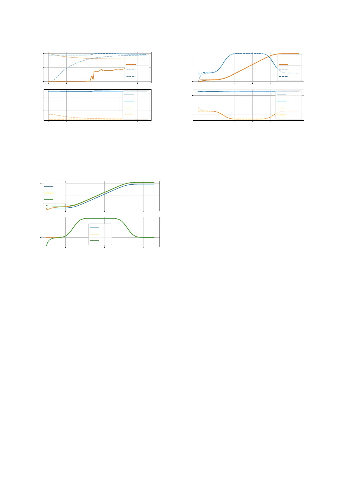
T o w ards mo del based con trol of the V ertical Gradien t F reeze crystal gro wth pro cess S. Ec kleb e a, ∗ , F. W oittennek b , J. Winkler a , Ch. F rank-Rotsch c , N. Dropk a c a Institute of Contr ol The ory, T e chnische Universit¨ at Dr esden, 01062 Dr esden, Germany b IACE, Private University for He alth Scienc es, Me dic al Informatics and T e chnolo gy (UMIT), Eduar d-Wal lno efer-Zentrum 1, A-6060 Hal l in Tir ol, A ustria c L eibniz Institute for Crystal Gr owth (IKZ), Max-Born-Str. 2, 12489 Berlin, Germany Abstract In this con tribution tracking control designs using output feedbac k are presented for a tw o-phase Stefan problem arising in the modeling of the V ertical Gradien t F reeze process. The tw o-phase Stefan problem, consisting of tw o coupled free b oundary problems, is a vital part of man y crystal gro wth processes due to the temporally v arying exten t of the solid and liquid domains during gro wth. After discussing the sp ecial needs of the pro cess, collo cated as well as flatness-based state feedbac k designs are carried out. T o render the setup complete, an observer design is p erformed, using a flatness-based appro ximation of the original distributed parameter system (DPS). The quality of the provided approximations as w ell as the p erformance of the op en and closed lo op control setups is analysed in several simulations. Keywor ds: V ertical Gradien t F reeze, Industrial Crystallization, Distributed Parameter Systems, Differential Flatness, Observ er Design 1. In tro duction The V ertical Gradien t F reeze (VGF) process is the most imp ortan t tec hnology for the pro duction of bulk comp ound semiconductor crystals lik e Gallium-Arsenide (GaAs) or Indium-Phosphide (InP) [1] which are esp ecially used for man ufacturing high-p ow er and high-frequency electronics as well as infrared ligh t-emitting and laser dio des. F or these purp oses the crystals ha ve to meet high requirements with resp ect to their purity and structural p erfection. The basic VGF setup is sho wn in Figure 1: A crucible, usually made of b oron nitride and holding the material whic h is to b e molten and then solidified, is surrounded b y several heaters. The whole setup is enclosed by a thick insulation. A t the b ottom of the crucible a seed crystal is placed which defines the orientation of the crystal to b e gro wn. After melting up the material in the crucible (with- out destro ying the seed crystal) the temp erature field has to b e adjusted and trac ked by means of the heat input of the heaters in suc h a wa y that the melt solidifies from the b ottom to the top in a desired manner. This means that a) the solid-liquid-interface (phase b oundary) maintains a plain shape and b) the gro wth rate (i.e., the v elo cit y of the solid-liquid-in terface) and the temp erature gradien t at the phase b oundary are kept on a certain level throughout the whole pro cess as they hav e b een identified as crucial fac- tors regarding the quality of the grown crystal (see eg. [2] for an analysis regarding the related Czo c hralski pro cess). This solidification by using a trav elling vertical temp era- ture gradient is where the name of the pro cess originates ∗ Corresponding author: stefan.ecklebe@tu-dresden.de Melt Crystal T op Heater Bottom Heater Seed Crucible Heater-Magnet- Mo dules Figure 1: Sketc h of a VGF crystal growth furnace. Pr eprint submitte d to arXiv.or g August 8, 2019 from. T o affect the pro cess, a top and a b ottom heater in form of plane disks, as well as three jack et heaters in form of coils are moun ted in the plant. Due to its imp ortance the improv emen t of this pro cess is in fo cus of the scientific comm unity , resulting e.g. in the application of external tra velling magnetic fields (TMFs) [3, 4, 5, 6]. How ev er, a topic that has not received m uch atten tion is the pro cess control of this growth technique. This lac k of cov erage has tw o main reasons: Firstly , in-situ measuremen ts from the gro wing crystal (e.g. the shape and p osition of the phase b oundary or the growth rate) as a prerequisite for feedback control are not av ailable or not applicable in an industrial environmen t [7]. Secondly , the coupled free b oundary problems for crystal and melt form a so called tw o-phase Stefan problem (SP) [8] which is of nonlinear nature. As is well known, the first issue can b e tackled by an appropriate observer design which has already b een pre- sen ted in [9] for the one-phase SP. How ev er, regarding the implemen tation a simulation mo del is needed for the ob- serv er. Since the sim ulation of solidification pro cesses and therefore of free b oundary problems (FBPs) has b een un- der in vestigation ov er the last decades, there are a lot of differen t numerical schemes like the Enthalp y[10], Level- Set[11] or Moving-Grid[12] method av ailable, to name just a few. How ever, b eing n umerical schemes, identifying their v ariables with a state-space representation for subsequent observ er design is not straight forward. The second issue is broadly discussed in the frame- w ork of DPSs. Making the assumption, that the temp er- ature distribution in one phase is constant (which is often justified due to its dominant spatial exten t) yields the so called one-phase SP. Regarding this sp ecial case, results are lately av ailable for the feedforward design [13] using flatness-, as w ell as for feedback designs using en thalpy- [14, 15], geometrically- [16] or backstepping- [17] based approac hes. Regarding the full problem, [18] e xtends the flatness-based motion planning to the t wo-phase SP, while [19] addresses the problem from the side of optimal con trol. Concerning feedbac k, a direct extension of the approaches for the one-phase case is not feasible since for the tw o- phase case, the coupling b et ween the tw o FBPs has to b e tak en into accoun t. In this context it is notew orthy that [20] already states a Lyapuno v-based con trol law for the t wo-phase SP with actuation at one b oundary . How ev er, according to our curren t knowledge there are no results a v ailable for the trac king control of the tw o-phase SP via output feedbac k concerning multiple inputs. 1.1. Obje ctive and structur e of the p ap er The main goal of this contribution is to in tro duce meth- o ds for tracking con trol of a one dimensional, t wo-phase SP via output feedback (resp. observer based state feed- bac k) as a starting p oin t for an improv emen t of pro cess con trol in the VGF growth pro cess. T o reach this goal, the pap er is structured as follows: In Section 2 the distributed parameter mo del of the pro- Γ l Γ s γ ( t ) z Melt Phase Crystal Boundary ϕ r Bottom Heater T op Heater Γ l − γ ( t ) Γ s − γ ( t ) 0 ˜ z Figure 2: Schematics of the cylindrical co ordinate system ( r , ϕ, z , t ), a meridional plane (blue) and the shifted coordinate ˜ z = z − γ ( t ). cess is introduced. Section 3 outlines a feedforward con- trol design which is based on the flat parametrisation of the solution by means of p o wer series. This feedforward subsequen tly serves as the source of a reference temp era- ture profile. Based on this, Section 4 introduces a collo- cated con troller that trac ks this reference by utilizing state feedbac k. Lo oking at the problem from another p oin t of view and further exploiting the flatness prop erty , Section 5 presen ts a flatness based state feedbac k control. This ap- proac h relies on a finite dimensional approximation of the system dynamics which is obtained from the parametrisa- tion in Section 3. T o comply with the sp ecific demands of the pro cess, different v arian ts of b oth control concepts are in troduced. Since all designs depend on state measure- men ts to some extend, in Section 6 a lump ed observer for the flat system appro ximation is sho wn. Section 7 presents sim ulation results for the different control setups using state and output feedback. Finally , a summary and an outlo ok to further work is given. 2. Mo delling of the VGF pro cess In this section a one dimensional distributed parameter mo del of the VGF pro cess plant is derived. F or this pur- p ose, the following simplifications are made: The crucible geometry is approximated b y a cylinder. Th us, the dis- tribution of the system temp erature T in the crucible de- p ends on the time t and the cylindrical co ordinates, given b y radius r , angle ϕ and height z , as depicted in Figure 2. F urthermore, any conv ectiv e effects in the melt are ne- glected. This is reasonable due to the dominating heat transp ort by diffusion. Bey ond, making use of the fact that the plant itself is rotationally symmetric to the lon- gitudinal axis, the mo del can b e reduced to a meridional plane of the crucible b y taking the a verage o ver the angular co ordinate ϕ . In addition, the lateral heaters are assumed to b e used as active isolation, av oiding an y heat loss in radial direction and therefore rendering the phase b ound- ary a horizon tal line. Hence, av eraging o ver the radius r allows further reduction of the domain to a line whose 2 b oundaries represen t the bottom and top of the crucible at z = Γ s and z = Γ l , resp ectively . Summarising, the system temp erature is given by T ( z , t ) for Γ s ≤ z ≤ Γ l and t > 0 while the phase b oundary is given by γ ( t ) ∈ (Γ s , Γ l ). This leads to the one dimensional nonlinear heat equa- tion [21] ∂ ∂ t  ρ ( T ( z , t )) c p ( T ( z , t )) T ( z , t )  = ∂ ∂ z  k ( T ( z , t )) ∂ ∂ z T ( z , t )  , z ∈ (Γ s , Γ l ) \ { γ ( t ) } (1) with the density ρ , the sp ecific heat capacity c p and k the thermal conductivit y b eing temp erature-dependent. As- suming piecewise constant parameters for the solid and the liquid phase it is p ossible to decomp ose the nonlinear system (1) into tw o FBPs for the temperatures T s ( z , t ) and T l ( z , t ): ∂ t T s ( z , t ) = α s ∂ 2 z T s ( z , t ) , z ∈ Ω s = (Γ s , γ ( t )) (2a) k s ∂ z T s (Γ s , t ) = δ s u s ( t ) (2b) T s ( γ ( t ) , t ) = T m (2c) ∂ t T l ( z , t ) = α l ∂ 2 z T l ( z , t ) , z ∈ Ω l = ( γ ( t ) , Γ l ) (2d) k l ∂ z T l (Γ l , t ) = δ l u l ( t ) (2e) T l ( γ ( t ) , t ) = T m . (2f ) Herein, the index “s” denotes the solid and the index “l” the liquid phase. The heat flows u s ( t ) and u l ( t ) at the b ottom and the top b oundary are considered as system inputs with the orientation factors δ s = − 1 and δ l = 1. The partial deriv ativ e of the quantit y T ( z , t ) with resp ect to z or t is denoted by ∂ z T ( z , t ) or ∂ t T ( z , t ). Finally , α s = k s ρ s c p , s and α l = k l ρ l c p , l denote the thermal diffusivities. Due to the moving phase b oundary latent heat is re- leased b y the solidification pro cess. This effect can b e mo delled by the Stefan condition [22] ρ m L ˙ γ ( t ) = k s ∂ z T s ( γ ( t ) , t ) − k l ∂ z T l ( γ ( t ) , t ) (3) with the density of the melt at melting temp erature ρ m and the sp ecific latent heat L . T ogether, the equations (2) and (3) form the t w o-phase SP whose state is giv en by x ( · , t ) =  T ( · , t ) γ ( t )  ∈ X = L 2 (Ω) × (Γ s , Γ l ) (4) with Ω = [Γ s , Γ l ]. Note that the PDE-ODE system defined b y (2) and (3) is inherently nonlinear since the domains of (2b) and (2e) dep end on the state v ariable γ ( t ). F ur- thermore, with the system b oundaries admitting access for measuremen ts, the system output is given by η ( t ) = h ( x ( t )) =  T (Γ s , t ) T (Γ l , t )  . (5) Exploiting the iden tical structure of the diffusion equa- tions, the following sections will – where applicable – re- sort to discuss merely one generic temp erature distribution T ◦ ( z , t ) for z ∈ Ω ◦ with ◦ to b e replaced by the indices s or l dep ending on the considered domain. 3. F eedforward control This section giv es a short recap of a feedforward control design which was presented in [13] for the one-phase and in [23] for the tw o-phase case to whic h the reader is kindly directed for further details. T o eliminate the temporal dep endency in the b oundary conditions of (2), the co ordinate transform ˜ T ◦ ( ˜ z , t ) = T ◦ ( z , t ) with ˜ z : = z − γ ( t ) (6) is introduced. As a consequence the phase b oundary is shifted into the origin of a new, moving reference frame as it can b e seen on the righ t-hand side of Figure 2. The resulting 1 system is giv en by ∂ t ˜ T ◦ ( ˜ z , t ) = α ◦ ∂ 2 ˜ z ˜ T ◦ ( ˜ z , t ) + ˙ γ ( t ) ∂ ˜ z ˜ T ◦ ( ˜ z , t ) (7a) k ◦ ∂ ˜ z ˜ T ( ˜ Γ ◦ ( t ) , t ) = δ ◦ u ◦ ( t ) (7b) ˜ T ◦ (0 , t ) = T m (7c) ˙ γ ( t ) = 1 Lρ m  k s ∂ ˜ z ˜ T s (0 , t ) − k l ∂ ˜ z ˜ T l (0 , t )  (7d) where ˜ Γ ◦ ( t ) : = Γ ◦ − γ ( t ). By expressing the solution ˜ T ◦ ( ˜ z , t ) of (7) in terms of a p o w er series in ˜ z : ˜ T ◦ ( ˜ z , t ) = ∞ X i =0 c ◦ ,i ( t ) ˜ z i i ! , (8) plugging it into (7a) and comparing the co efficients of lik e p o w ers of ˜ z the recursion formula c ◦ ,i +2 ( t ) = 1 α ◦  ∂ t c ◦ ,i ( t ) − ˙ γ ( t ) c ◦ ,i +1 ( t )  i = 0 , . . . , ∞ (9) is obtained. A closer examination of (8) sho ws that the follo wing holds for the initial co efficien ts : c ◦ , 0 ( t ) = ˜ T ◦ (0 , t ) = T m , c ◦ , 1 ( t ) = ∂ ˜ z ˜ T ◦ (0 , t ) . (10) By utilizing the Stefan condition (7d) solved for the gra- dien t at the liquid side ∂ ˜ z ˜ T l (0 , t ) = 1 k l  k s ∂ ˜ z ˜ T s (0 , t ) − ρ m L ˙ γ ( t )  (11) it follo ws that the solution for b oth phases can b e ex- pressed b y the gradient in the solid ∂ ˜ z ˜ T s (0 , t ) and the gro wth rate ˙ γ ( t ). Th us, the system (2) is differen tially flat with a flat output y ( t ) =  y 1 ( t ) y 2 ( t )  =  ∂ ˜ z ˜ T s (0 , t ) γ ( t )  . (12) Assuming conv ergence and truncating the series (8) at an order N , the mapping ˜ T N ( ˜ z , t ) =  ˜ T N s ( ˜ z , t ) ˜ T N l ( ˜ z , t )  = Θ N  ∂ ˜ z ˜ T s (0 , t ) , . . . , ∂ ˜ z ˜ T ( α 1 ) s (0 , t ) , γ ( t ) , . . . , γ ( α 2 ) ( t )  (13) 1 F or details see Appendix A.1. 3 where α 1 = b N / 2 c − 1 and α 2 = b N / 2 c can b e form ulated. Finally , choosing the tra jectories for the comp onen ts of y ( t ) as y ( t ) = y A + ( y B − y A ) φ  t ϑ  (14) where φ ( τ ) = 1 2  1 + tanh  2(2 τ − 1) (4 τ (1 − τ )) σ  (15) is of Gevrey-order α G = 1 + 1 σ [24] con vergence of the sc heme can b e sho wn for α G ≤ 2 [18]. Hence, by utilizing the b oundary condition (7b) the inputs u s ( t ) and u l ( t ) are obtained b y ev aluating the tem- p erature profile which is given the mapping (13). This yields the input map u ( t ) = Φ N ( y 1 ( t ) , . . . , y ( α 1 ) 1 ( t ) , y 2 ( t ) , . . . , y ( α 2 ) 2 ( t )) (16) giv en in terms of the flat output. Summarising, by prescribing reference tra jectories y r ( t ) for the flat output y ( t ), a reference temp erature distribu- tion T r ( z , t ) and input u r ( t ) can b e computed. These re- sults will serve as the basis for the con trol design in the next section. 4. Collo cated feedback This section will presen t an approach for the collocated trac king control of the tw o-phase SP. T o do this, differ- en t con trol errors are compared concerning their suitabil- it y concerning the V GF pro cess and the stability of the closed lo op is inv estigated. In detail, the profile T r ( z , t ), in tro duced in the previous section, will b e utilised as con- trol reference while the input tra jectories u r ( t ) are not needed. Note that all considerations in this section are conducted in the original spatially fixed co ordinates. 4.1. Err or definitions Cho osing the distributed temp erature error e ( z , t ) : = T ( z , t ) − T r ( z , t ) (17) as deviation of the system temp erature T ( z , t ) from the reference profile T r ( z , t ) ov er the complete spatial domain as in [20] seems natural at a first glance. How ev er, this is not useful in order to meat the tec hnological requiremen ts: Due to the biphasic character of the system, conv ergence of e ( z , t ) into the origin implies conv ergence of the phase b oundary p osition error ∆ γ ( t ) = γ ( t ) − γ r ( t ) . (18) Ho wev er, the qualit y of the crystal does not dep end on the p osition of the phase b oundary but rather on its velocity . Moreo ver, it seems more natural to compare the temp er- ature of like phases only . As a consequence the error is defined on the basis of a shifted reference tra jectory ˜ e ( z , t ) : = T ( z , t ) − T r ( z − ∆ γ ( t ) , t ) (19) in combination with (18). T o do so, how ev er, the planning for the reference profile T r ( z , t ) has to b e carried out on an extended spatial domain. More precisely , for any admissi- ble ∆ γ ( t ), the profile T r ( z − ∆ γ ( t ) , t ) must not b e ev alu- ated outside of its domain. Considering the plant prop er- ties, it follows that ∆ γ ( t ) ∈ (Γ s − Γ l , Γ l − Γ s ). Therefore, a feasible domain for T r ( z , t ) w ould b e ( z , t ) ∈ Ω r × R + , with Ω r = [2Γ s − Γ l , 2Γ l − Γ s ]. Analysing 2 (19), the phase dep en- den t tracking error ˜ e ◦ ( z , t ) = T ◦ ( z , t ) − T ◦ , r ( z − ∆ γ ( t ) , t ) is go verned by ∂ t ˜ e ◦ ( z , t ) = α ◦ ∂ 2 z ˜ e ◦ ( z , t ) + ∆ ˙ γ ( t ) ∂ z T ◦ , r ( z − ∆ γ ( t ) , t ) z ∈ Ω ◦ (20a) ∂ z ˜ e ◦ (Γ ◦ , t ) = δ ◦ k ◦ u ( t ) − ∂ z T ◦ , r (Γ ◦ − ∆ γ ( t ) , t ) (20b) ˜ e ◦ ( γ ( t ) , t ) = 0 (20c) ∆ ˙ γ ( t ) = 1 Lρ m ( k s ˜ e s ( γ ( t ) , t ) − k l ˜ e l ( γ ( t ) , t )) . (20d) Herein, the second term in the rigth-hand side of (20b) can b e understoo d as a feedforward part. Ho wev er, it do es not coincide with the reference input u r ( t ) due to the spatial shift. Finally , the error state is given by ξ ( z , t ) =  ˜ e ◦ ( z , t ) ∆ γ ( t )  ∈ X. (21) 4.2. Contr ol law A very intuitiv e wa y to manipulate the system is to con vert (20b) into ∂ z ˜ e ◦ (Γ ◦ , t ) = − δ ◦ κ ◦ ˜ e ◦ (Γ ◦ , t ) . (22) This leads to the feedbac k law u ◦ ( t ) = k ◦ δ ◦ ∂ z T ◦ , r ( z − ∆ γ ( t ) , t ) − κ ◦ k ◦ ˜ e ◦ (Γ ◦ , t ) . (23) Alb eit reasonable in its comp osition, the control law only honours the b oundary error at z = Γ ◦ . Hence, further analysis is required to ensure con vergence of ∆ ˙ γ ( t ). 4.3. Stability analysis Although the framew ork which will b e applied here was already laid out in [25] for finite dimensional systems, the nomenclature, used in the following is b orro wed from [26] due to its application for the infinite dimensional case. Keeping in mind that the tracking of the growth velocity ˙ γ ( t ) is more imp ortant than the exact adjustment of the b oundary p osition γ ( t ), it is apparent that to obtain the desired results, ξ ( z , t ) may not necessarily con verge in to the origin but rather into a compact subset of the state space, giv en by A : =  ( ξ , γ ) T ∈ X | ξ = 0  (24) 2 Details in App endix A.2. 4 with X from (4). Assuming that ξ ( z , t ) ∈ A for some t , (20d) yields that ∆ ˙ γ ( t ) = 0. Using this information, (20a) gives ∂ t ˜ e ( z , t ) = 0. Thus ξ ( z , 0) ∈ A = ⇒ ξ ( z , t ) ∈ A ∀ t ≥ 0, rendering A an inv ariant set of the system (20). F urthermore let the distance of an element x ∈ X to A b e giv en by | x | A : = min {k x − y k X | y ∈ A} and consider the function classes: K : = { f : R + 7→ R + | f (0) = 0 , f is contin uous and strictly increasing } K ∞ : = { f ∈ K| f is unbounded } . As stated in [26], if there exists a Lyapuno v function V ( ξ ) 3 , so that a 1 ( | ξ | A ) ≤ V ( ξ ) ≤ a 2 ( | ξ | A ) ∀ ξ ∈ X (25a) ˙ V ( ξ ) ≤ − b ( | ξ | A ) ∀ ξ ∈ X (25b) with a 1 , a 2 ∈ K ∞ and b ∈ K hold, the system (20) is uniformly globally asymptotically stable with resp ect to A . F or this purp ose, the Lyapuno v function candidate V ( ξ ) = 1 2 Γ l Z Γ s ˜ e 2 ( z , t ) d z (26) is used, which fulfils condition (25a). F urthermore, in the first part of App endix B it is shown that for a simplified reference profile T r ( z , t ), the candidate (26) satisfies (25b). Th us, rendering it a Lyapuno v function for (20) with re- sp ect to A . Softening those demands on T r ( z , t ) is possible but leads to stricter requirements for the phase b oundary error ∆ γ ( t ), which are again hard to show for the general case. The detailed steps are giv en in in the second part of App endix B. Ho wev er, sim ulation results show that the system state ξ con verges to A for non-trivial reference profiles, to o. 5. Distributed F eedback Exploiting the fact that parametrisation of the system (2)-(3) whic h is introduced in Section 3 is differen tially flat [13, 18] with the flat output (12), this prop ert y can b e used to design a feedback in a straight-forw ard fashion without the explicit computation of a reference temp erature profile. 5.1. System State In [27, Ch. 5] a state space representation for a diffu- sion equation is given by means of the series co efficients of a p ow er approximation. Therein, the comp onents of a new state ζ N ◦ ( t ) : = ( c ◦ , 1 ( t ) , . . . , c ◦ ,N ( t )) T b elong to an appro ximation of an order N . Instead of extending this 3 F or b etter readability , in the following the arguments of ξ ( z , t ) are omitted. approac h b y com bining the co efficients of the solid and liq- uid approximations into an extended state vector ¯ ζ N ( t ) =  x N T s ( t ) , x N T l ( t )  T one may directly use the appropriate deriv ativ es of the flat output. Hence, the state comp o- nen ts χ N n ( t ) , 1 ≤ n ≤ M with M = ( α 1 + α 2 + 2) in flat co ordinates constitute the state v ector χ N ( t ) ∈ R M whic h reads: χ N ( t ) =  y 1 ( t ) , . . . , y ( α 1 ) 1 ( t ) , y 2 ( t ) , . . . , y ( α 2 ) 2 ( t )  T . (27) Herein, the required deriv ativ es can b e obtained from the iterated recursion formulas for b oth phases, cf. (9), for clarit y condensed in the map χ N ( t ) = ψ N  ¯ ζ N ( t )  . (28) Th us, examining the comp onen ts of the deriv ativ e ˙ χ N ( t ) t wo integrator chains b ecome apparent: ˙ χ N n ( t ) = ( y ( n ) 1 ( t ) for 1 ≤ n ≤ α 1 + 1 y ( n − ( α 1 +1)) 2 ( t ) for α 1 + 1 < n ≤ M . (29) Herein, the yet unknown deriv ativ es y ( α 1 +1) 1 and y ( α 2 +1) 2 can b e obtained from an extended version of (28) b y using the extended co efficien t state ¯ ζ N +1 ( t ): χ N +1 ( t ) = ψ N +1  ¯ ζ N +1 ( t )  . (30) Ho wev er this mapping requires the co efficien ts c s ,N +1 ( t ) and c l ,N +1 ( t ). F ortunately , these can b e acquired from the resp ectiv e b oundary conditions of b oth phases, cf. (7b), after inserting the series expansion c ◦ ,N +1 ( t ) = N ! Γ N ◦ k ◦ δ ◦ u ◦ ( t ) − N − 1 X i =0 c ◦ ,i +1 ( t ) ˜ z i i ! ! (31) wherein the co efficien ts c ◦ , 1 ( t ) to c ◦ ,N ( t ) can readily be computed from χ N ( t ). According to (5), the outputs of eac h phase are given by η ◦ ( t ) = ˜ T ◦ ( ˜ Γ ◦ ( t ) , t ) = N X i =0 c ◦ ,i ( t ) ˜ Γ ◦ ( t ) i i ! . (32) Hence, by using ¯ ψ N ( · ), the inv erse of the map (28), the output can b e written as η flat ( t ) = h flat  ¯ ψ N  χ N ( t )   . (33) 5.2. F e e db ack Design Regarding y 1 ( t ) and y 2 ( t ) as the outputs of the system, the trac king errors ε j ( t ) = y j ( t ) − y j, r ( t ) , j = 1 , 2 (34) 5 are defined. Hence, the decoupled linear error dynamics ε ( α 1 +1) 1 ( t ) = − α 1 X i =0 κ 1 ,i ε ( i ) 1 ( t ) (35a) ε ( α 2 +1) 2 ( t ) = − α 2 X i =0 κ 2 ,i ε ( i ) 2 ( t ) (35b) are prescrib ed by c ho osing appropriate co efficien ts κ 1 and κ 2 . Defining the new inputs v 1 ( t ) : = y ( α 1 +1) 1 ( t ) and v 2 ( t ) : = y ( α 2 +1) 2 ( t ), b y using the inv erse of (30) ¯ ζ N +1 ( t ) = ¯ ψ N +1  χ N ( t ) , ( v 1 ( t ) , v 2 ( t )) T  , (36) the extended series co efficient set can be computed. Lastly , ev aluation of (16) yields the control input u ( t ). Ho wev er, this design inherits the problem that an al- ready gro wn crystal will b e remelted if the measured in ter- face p osition is ahead of the reference. Therefore, in view of the shifted error system (19), the pair ( y 1 ( t ) , ˙ y 2 ( t )) may b e regarded as the output of a mo dified system, yielding ˜ ε 2 ( t ) = ˙ y 2 ( t ) − ˙ y 2 , r ( t ) as w ell as the dynamics ˜ ε ( α 2 ) 2 ( t ) = − α 2 − 1 X i =0 ˜ κ 2 ,i ˜ ε ( i ) 2 ( t ) (37) instead of (35b). Th us, a mo dified virtual input can b e stated as ˜ v 2 ( t ) : = ˜ ε ( α 2 ) 2 ( t ) + y ( α 2 +1) 2 , r ( t ) whic h, by using (36) and (16) with ˜ v 2 ( t ) instead of ˜ v 2 ( t ), yields the mo dified con trol input ˜ u ( t ). 6. Observ er Design This section p erforms an observer design as sho wn in [28], ho wev er in this case based on the flat system state (27). The estimated system with the state ˆ x ( t ) is given b y the cop y ˙ ˆ x ( t ) = f ( ˆ x ( t ) , u ( t )) + L ( t ) ¯ η ( t ) (38a) ˆ η ( t ) = h ( ˆ x ( t )) (38b) with L ( t ) to b e chosen later on and ¯ η ( t ) = ˆ η ( t ) − η ( t ). The plan t mo del (38) is extended in the following w ay: ˙ x ( t ) = f ( x ( t ) , u ( t ) + µ ( t )) , η ( t ) = h ( x ( t ) + ν ( t )) . (39) Herein, µ ( t ) and ν ( t ) represent disturbances acting on the system input and output, resp ectively . F urthermore, de- noting ¯ x ( t ) = ˆ x ( t ) − x ( t ), the observ er error dynamics ˙ ¯ x ( t ) = f ( ˆ x ( t ) , u ( t )) + L ( t ) ¯ η ( t ) − f ( x ( t ) , u ( t ) − µ ( t )) (40a) ¯ η ( t ) = h ( ˆ x ( t )) − h ( x ( t ) − ν ( t )) (40b) is obtained. In the following, the computation of L ( t ) will b e p erformed on a linearisation of (40) along the reference tra jectory y r ( t ), giv en by: ˙ ¯ x ( t ) = A ( t ) ¯ x ( t ) − B ( t ) µ ( t ) + L ( t ) ¯ η ( t ) (41a) ¯ η ( t ) = C ( t ) ( ¯ x ( t ) − ν ( t )) . (41b) By defining the cost functional J = ¯ x T (0) S ¯ x (0) + t Z 0 µ T ( t ) Rµ ( t ) + ¯ η T ( t ) Q ¯ η ( t ) d t (42) where S ∈ R M × M and R , Q ∈ R 2 × 2 denote p enalties con- cerning the initial error as well as the disturbances on in- put and output, respectively . As [29, Th. 40, p.378] states, using the solution Π ( t ) ∈ R M × M of the Filtering Riccati Differen tial Equation (FDRE) ˙ Π ( t ) = Π ( t ) A T ( t ) + A ( t ) Π ( t ) − Π ( t ) C T ( t ) QC ( t ) Π ( t ) + B ( t ) R − 1 B T ( t ) (43a) with the initial condition Π (0) = S − 1 , (43b) the c hoice L ( t ) : = − Π ( t ) C T ( t ) Q (44) yields the optimal estimation for (41) regarding (42). Note that the solution of (43) can b e done in adv ance. 7. Results The theoretical results of the previous sections will no w b e ev aluated by simulations. A finite element method (FEM) approximation using the b oundary-immobilisation metho d will serve as a simulation mo del to compare the differen t feedbac k designs on a process orien ted b enc hmark from the V GF pro cess. The corresp onding parameters are giv en in T able 1. 7.1. Setup and fe e dforwar d F or the tra jectory planning, the following initial situ- ation is assumed: The phase b oundary is resting ( ˙ γ (0) = 0 m s − 1 ) at γ (0) = 0 . 2 m. F urthermore, as a result of a pre- vious step (as shown in [18]) a gradient of ∂ t T s ( γ (0) , 0) = 17 K cm − 1 has b een established at the solid side of the phase b oundary . Now, the gro wth pro cess is p erformed by prescribing γ r ( t ). Figure 3 shows the generated tra jecto- ries for ∂ t T s , r ( γ r ( t ) , t ) and γ r ( t ) as well as the calculated system inputs u s ( t ) and u l ( t ). 7.2. F e e db ack T o emulate a real gro wth pro cess, an initial error of γ e (0) = 100 mm and ˙ γ e (0) = − 3 mm h − 1 is introduced to the test-setup. T o gain an extensiv e o v erview, t wo v ersions of the collo cated controller from Section 4 are ev aluated, one using the fixed error definition from (17) and one using the shifted error from (19). F urthermore, t w o v ariants 4 The given unit refers to the second argument 6 T able 1: Parameters of the System Name Sym b ol V alue (s/l) Unit Sp ec. heat cap. c p 423 . 59 / 434 J kg − 1 K − 1 Therm. conduct. k 7 . 17 / 17 . 8 W m − 1 K − 1 Therm. diffus. α s 3 . 27 · 10 − 6 / m 2 s − 1 α l 7 . 19 · 10 − 6 m 2 s − 1 Densities ρ s 5171 . 24 / kg m − 3 ρ l 5702 . 37 kg m − 3 ρ m 5713 . 07 kg m − 3 Melting temp. T m 1511 . 15 K Sp ec. latent heat L 668 . 5 · 10 3 J kg − 1 Left Boundary Γ s 0 m Righ t Boundary Γ l 0 . 4 m F eedf. Appr. Order N ff 10 Obs. Appro x. Order N ob 5 Con t. Approx. Order N fb 5 Inp. W eigh t Mat. R 1 · 10 − 4 I 2 m 4 W − 2 s − 1 Out. W eigh t Mat. Q 1 · 10 − 4 I 2 K − 2 s − 1 Inp. dist. µ ( t ) = N (0 , 100) 4 kW 2 m − 4 Output dist. ν ( t ) = N (0 , 10) 4 K 2 Init. W eigh t Mat. S 1 · 10 − 3 I 5 m 2 K − 2 Sim. Disc. No des N fem 41 200 250 300 γ ( t ) / mm γ r ( t ) 0 5 10 15 20 25 t / h − 10 0 10 u ( t ) / kW m − 2 u rl ( t ) u rs ( t ) 5 10 15 ∂ z T r ( γ r ( t ) , t ) / K cm − 1 ∂ z T s ( γ − r ( t ) , t ) ∂ z T l ( γ + r ( t ) , t ) Figure 3: Reference tra jectories for gradients and phase b oundary (top) as well as the generated heater tra jectories for the system in- puts (b ottom) of the feedforward control. t / h 0 5 10 15 20 25 z / mm 0 100 200 300 400 T r ( z , t ) / K 1000 1100 1200 1300 1400 1500 1600 Figure 4: Calculated reference temp erature profile T r ( z , t ) with the reference phase b oundary tra jectory γ r ( t ) (blue). of the distributed con troller from Section 5 are analysed, using the standard (34) and mo dified tracking error (37). As Figure 5a shows, the “fixed” collo cated feedback (orange, solid) successfully corrects the initial error in the phase b oundary p osition and tracks the reference. T o do this how ev er, a part of the already grown crystal has to b e remolten which is to b e av oided. In contrast, the col- lo cated feedback with the shifted error system (orange, dashed) ignores the error in γ ( t ) and makes no attempts on remelting the crystal. F urthermore, in Figure 5b it can b e seen that this v ariant corrects the growth rate error faster than its fixed counterpart. How ev er, a drawbac k that remains for this controller is that due to the simple reference shifting, a larger crystal is obtained at the end of the pro cess if no further logic is sup erimp osed. No w to the standard v ariant of the distributed feed- bac k (green, solid). As it can b e seen in Figure 5a, the error in γ ( t ) is successfully corrected and the growth tar- get is reached. Nevertheless, Figure 5b sho ws a severe spik e in the growth rate, originating from the swift cor- rection of γ ( t ), thus remelting the crystal. Opp osed to this, the version with the mo dified tracking error (green, dashed) tolerates the initial deviation in γ ( t ) and contin- ues tracking the tra jectory of ˙ γ ( t ). Ho w ever, as for the shifted v ariant of the collo cated feedback, the deviation in γ ( t ) still app ears at the end. The control parameters for these sim ulations can b e found in App endix D. 7.3. Observer T o analyse the observer p erformance a system under pure feedforward control is considered. F or this case, the initial state estimate ˆ χ N (0) of the observ er is sp ecified using the reference tra jectory y r (0). T o examine the ro- bustness against disturbances, the real system starts with the initial errors γ e (0) = 100 mm and ˙ γ e (0) = − 3 mm h − 1 for b oth, the crystallisation interface and the growth rate, resp ectiv ely . F urthermore, the pro cess disturbances µ ( t ) and ν ( t ) are realised b y zero-mean normal distributed noise, distorting the input and output measurements as illus- trated in Figure 6. As Figure 7b displays, the state esti- mate quickly conv erges against the real one and the system state is prop erly track ed afterw ards. Due to the different scales of the comp onen ts in χ N ( t ), in ternally a scaled ver- sion ˜ χ N ( t ) = T N χ N ( t ) has b een used, with T N giv en in App endix D. 7.4. Complete c ontr ol system T o examine the p erformance of the feedback controller when supplied with the state estimates from the observer instead of the real system state, a similar setup is used. P articularly , the estimate is generated by an observer of t yp e (39) which is using the mo del introduced in Subsec- tion 5.1. By wa y of example, the distributed feedbac k con troller with mo dified tracking error is used to close the con trol lo op. As the b ottom plot in Figure 8 shows, the closed lo op p erforms as exp ected. 7 0 5 10 15 20 25 t / h 200 220 240 260 280 300 γ ( t ) / mm (a) Phase b oundary p osition 0 5 10 15 20 25 t / h − 15 − 10 − 5 0 5 ˙ γ ( t ) / mm h − 1 (b) Growth velocity Figure 5: Comparison of the tracking b eha viour of the reference (blue) b etw een collo cated (orange) and distributed feedbac k (green) using the original (solid) or mo dified error (dashed), resp ectively . Note that the orange and green dashed lines are nearly equal. 5 10 u l ( t ) / kW m − 2 u l ( t ) + µ l ( t ) ˆ u l ( t ) 0 5 10 15 20 25 t / h 1600 1700 y l ( t ) / K y l ( t ) + ν l ( t ) ˆ y l ( t ) − 14 − 13 − 12 u s ( t ) / kW m − 2 u s ( t ) + µ s ( t ) ˆ u s ( t ) 1200 1300 y s ( t ) / K y s ( t ) + ν s ( t ) ˆ y s ( t ) Figure 6: Inputs (top) and outputs (b ottom) of the original system (dark) and their disturbed coun terparts (light), used by the observ er. 8. Conclusion and outlo ok In this contribution, reference tracking control strate- gies for the V GF pro cess, mo delled as a tw o-phase SP ha ve b een presented. Based on the pro cess demands not to remelt the already solidified domain, tw o different con- trol approaches hav e b een dev elop ed. The p erformance of comp onen ts of the control system has b een prov en by a sim ulation study . A drawbac k of the prop osed solutions is the conv er- gence of the utilised series for smaller transition times. While this is not a problem for the growth of GaAs, it ma y cause complications for the pro duction of other mate- rials. A direct alternativ e would be to use so called ( N , ξ )- appro ximate k -sums as introduced in [30]. How ev er, an- other promising approach is the control via a time-v arian t bac kstepping transformation c.f [31] which is curren tly un- der in vestigation and will b e cov ered in a forthcoming pub- lication. Ac kno wledgments This w ork has b een funded b y the Deutsche F orsch ungs- gemeinsc haft (DFG) [pro ject num bers WI 4412/1-1, FR 3671/1-1]. References [1] M. Jurisch, F. B¨ orner, T. B¨ unger, S. Eichler, T. Flade, U. Kret- zer, A. K¨ ohler, J. Stenzenberger, B. W einert, LEC- and VGF- growth of SI GaAs single crystals—recent developmen ts and current issues, Journal of Crystal Gro wth 275 (1) (2005) 283 – 291, proceedings of the 14th International Conference on Crys- tal Growth and the 12th International Conference on V apor Growth and Epitaxy . doi:10.1016/j.jcrysgro.2004.10.092 . [2] J. V anhellemon t, The v/g criterion for defect-free silicon sin- gle crystal growth from a melt revisited: Implications for large diameter crystals, Journal of Crystal Gro wth 381 (2013) 134 – 138. doi:https://doi.org/10.1016/j.jcrysgro.2013.06.039 . [3] C. F rank-Rotsc h, N. Dropk a, A. Glacki, U. Juda, VGF growth of GaAs utilizing heater-magnet mo dule, Journal of Crystal Growth 401 (2014) 702–707. [4] N. Dropka, C. F rank-Rotsch, Accelerated VGF-crystal growth of GaAs under trav elling magnetic fields, Journal of Crystal Growth 367 (2013) 1–7. [5] N. Dropk a, C. F rank-Rotsch, Enhanced VGF-GaAs gro wth us- ing pulsed unidirectional TMF, Journal of Crystal Growth 386 (2014) 146 – 153. doi:10.1016/j.jcrysgro.2013.09.027 . [6] N. Dropk a, C. F rank-Rotsch, GaAs -– vertical gradient freeze process intensification, Crystal Growth and Design 14 (2014) 5122–5130. [7] P .W ellmann, G. Neubauer, L. F ahlbusc h, M. Salamon, N. Uhlmann, Growth of SiC bulk crystals for application in power electronic devices – pro cess design, 2D and 3D X-ray in situ visualization and adv anced doping, Cryst. Res. T ec hnol. 50 (2015) 2–9. [8] J. Crank, F ree and Mo ving Boundary Problems (Oxford Science Publications), Oxford Science Publications, Oxford University Press, 1984. [9] S. Koga, M. Diagne, M. Krstic, Output feedback con trol of the one-phase Stefan problem, in: 2016 IEEE 55th Conference on Decision and Control (CDC), 2016, pp. 526–531. doi:10.1109/ CDC.2016.7798322 . 8 200 205 210 y 2 ( t ) / mm y 2 ( t ) ˆ y 2 ( t ) 0 . 0 0 . 5 1 . 0 1 . 5 2 . 0 2 . 5 t / h 1000 1500 y 1 ( t ) / K m − 1 y 1 , s ( t ) ˆ y 1 , s ( t ) y 1 , l ( t ) ˆ y 1 , l ( t ) − 2 0 ˙ y 2 ( t ) / mm h − 1 ˙ y 2 ( t ) ˙ ˆ y 2 ( t ) (a) Beginning 200 250 300 y 2 ( t ) / mm y 2 ( t ) ˆ y 2 ( t ) 0 5 10 15 20 25 t / h 500 1000 1500 y 1 ( t ) / K m − 1 y 1 , s ( t ) ˆ y 1 , s ( t ) y 1 , l ( t ) ˆ y 1 , l ( t ) 0 5 ˙ y 2 ( t ) / mm h − 1 ˙ y 2 ( t ) ˙ ˆ y 2 ( t ) (b) Complete simulation Figure 7: Estimates from the observer (dark), compared to the evolution of the real system’s v ariables (light) for the phase b oundary and growth rate (top) as well as the gradients at the phase b oundary for crystal and melt. 200 250 300 γ ( t ) / mm γ r ( t ) ˆ γ ( t ) γ ( t ) 0 5 10 15 20 25 t / h 0 5 ˙ γ ( t ) / mm h − 1 ˙ γ r ( t ) ˆ ˙ γ ( t ) ˙ γ ( t ) Figure 8: Resulting tra jectories of the phase b oundary (top) and the growth rate (bottom) for the complete control lo op with distributed output feedback (green), compared to the reference (blue) and the estimated (orange). [10] J. Brusche, A. Segal, C. V uik, H. Urbach, A comparison of en- thalpy and temp erature metho ds for melting problems on com- posite domains, Numerical Mathematics and Adv anced Appli- cations. [11] S. Chen, B. Merriman, S. Osher, P .Smerek a, A simple level set method for solving Stefan problems, Journal of Computational Physics. [12] G. Beck ett, J. A. Mack enzie, M. L. Rob ertson, A moving mesh finite element method for the solution of two-dimensional Ste- fan problems, Journal of Computational Physics doi:10.1006/ jcph.2001.6721 . [13] W. B. Dunbar, N. Petit, P . Rouchon, P . Martin, Motion plan- ning for a nonlinear Stefan problem, European Series in Applied and Industrial Mathematics (ESAIM): Control, Optimization and Calculus of V ariations 9 (2003) 275–296. [14] B. Petrus, J. Bentsman, B. Thomas, Enthalp y-based feedback control algorithms for the Stefan problem, in: Pro ceedings of the IEEE Conference on Decision and Control, 2012, pp. 7037– 7042. [15] B. Petrus, J. Ben tsman, B. G. Thomas, Application of en thalp y- based feedback control metho dology to the tw o-sided stefan problem, in: 2014 American Control Conference, 2014, pp. 1015–1020. doi:10.1109/ACC.2014.6859062 . [16] A. Maidi, J.-P . Corriou, Boundary geometric control of a linear Stefan problem, Journal of Pro cess Control 24 (6) (2014) 939 – 946, energy Efficient Buildings Sp ecial Issue. doi:https:// doi.org/10.1016/j.jprocont.2014.04.010 . [17] S. Koga, M. Diagne, S. T ang, M. Krstic, Backstepping control of the one-phase Stefan problem, in: 2016 American Control Con- ference (ACC), 2016, pp. 2548–2553. doi:10.1109/ACC.2016. 7525300 . [18] J. Rudolph, J. Winkler, F. W oittennek, Flatness based tra- jectory planning for tw o heat conduction problems in crys- tal growth technology , e-ST A (Sciences et T echnologies de l’Automatique) 1 (1). [19] M. Hinze, O. P¨ atzold, S. Ziegenbalg, Solidification of a gaas melt—optimal control of the phase in terface, Journal of Crystal Growth 311 (8) (2009) 2501 – 2507. doi:https://doi.org/10. 1016/j.jcrysgro.2009.02.031 . [20] B. Petrus, J. Bentsman, B. G. Thomas, F eedbac k control of the tw o-phase Stefan problem, with an application to the contin u- ous casting of steel, in: 49th IEEE Conference on Decision and Control (CDC), 2010, pp. 1731–1736. doi:10.1109/CDC.2010. 5717456 . [21] J. R. Cannon, The One-Dimensional Heat Equation, V ol. 23 of Encyclop edia of Mathematics and its Applications, Addison- W esley , 1984. [22] J. Stefan, ¨ Uber die Theorie der Eisbildung, insb esondere ¨ uber die Eisbildung in Polarmeere, Annalen der Ph ysik alischen Chemie (1891) 269–286. [23] J. Rudolph, J. Winkler, F. W oittennek, Flatness based con- trol of distributed parameter systems: Examples and com- puter exercises from v arious tec hnological domains, Beric hte aus der Steuerungs- und Regelungstechnik, Shaker V erlag, Aachen, 2003. [24] M. Gevrey , Sur la nature analytique des solutions des ´ equations aux d´ eriv´ ees partielles. premier m´ emoire, Annales scientifiques de l’ ´ Ecole Normale Sup´ erieure 35 (1918) 129–190. URL http://eudml.org/doc/81374 [25] V. I. Zubov, Methods of A.M. Lyapuno v and their application, P . No ordhoff, Groningen, 1964. [26] A. Mironchenk o, F. Wirth, A non-co erciv e Ly apuno v framework for stability of distributed parameter systems, in: 2017 IEEE 56th Annual Conference on Decision and Control (CDC), 2017, pp. 1900–1905. doi:10.1109/CDC.2017.8263927 . [27] T. Meurer, F eedforw ard and feedback tracking control of diffusion-conv ection-reaction systems using summability meth- ods, Ph.D. thesis, Universit y of Stuttgart (2005). doi:http: //dx.doi.org/10.18419/opus- 4075 . [28] T. Meurer, M. Zeitz, F eedforward and feedback tracking con- trol of nonlinear diffusion–conv ection–reaction systems using summability metho ds, Industrial & Engineering Chemistry Re- 9 search 44 (8) (2005) 2532–2548. arXiv:https://doi.org/10. 1021/ie0495729 , doi:10.1021/ie0495729 . URL https://doi.org/10.1021/ie0495729 [29] E. D. Son tag, Mathematical Control Theory , 2nd Edition, V ol. 6 of T exts in Applied Mathematics, Springer-V erlag, 1998. [30] T. Meurer, M. Zeitz, Flatness-based feedback control of diffusion-conv ection-reaction systems via k-summable p ow er se- ries, IF AC Pro ceedings V olumes 37 (13) (2004) 177 – 182, 6th IF AC Symp osium on Nonlinear Control Systems 2004 (NOL- COS 2004), Stuttgart, Germany , 1-3 September, 2004. doi: https://doi.org/10.1016/S1474- 6670(17)31219- 3 . [31] T. Meurer, A. Kugi, T racking control for b oundary controlled parabolic p des with varying parameters: Combining backstep- ping and differential flatness, Automatica 45 (5) (2009) 1182 – 1194. doi:https://doi.org/10.1016/j.automatica.2009.01. 006 . URL http://www.sciencedirect.com/science/article/pii/ S0005109809000478 [32] A. S. Mirosla v Krstic, Boundary control of PDEs: a course on backstepping designs, siam Edition, Adv ances in Design and Control, So ciety for Industrial and Applied Mathematic, 2008. App endix A. T ransformations App endix A.1. Moving r efer enc e system The co ordinate transform ˜ T ( ˜ z , t ) = T ( z , t ) with ˜ z : = z − γ ( t ) T aking the partial deriv ativ e w.r.t. z gives ∂ 2 z T ( z , t ) = ∂ 2 ˜ z ˜ T ( ˜ z , t ) (A.1) while according to the chain rule, the time deriv ativ e b e- comes ∂ t T ( z , t ) = d d t  ˜ T ( ˜ z , t )  = ∂ ˜ z ˜ T ( ˜ z , t ) ∂ t ˜ z ( t ) + ∂ t ˜ T ( ˜ z , t ) = − ∂ ˜ z ˜ T ( ˜ z , t ) ˙ γ ( t ) + ∂ t ˜ T ( ˜ z , t ) (A.2) where ˙ γ ( t ) denotes the growth rate. Inserting (A.2) and (A.1) in to (2) yields the transformed generic system ∂ t ˜ T ( ˜ z , t ) = α ◦ ∂ 2 ˜ z ˜ T ( ˜ z , t ) + ˙ γ ( t ) ∂ ˜ z ˜ T ( ˜ z , t ) k ◦ ∂ ˜ z ˜ T (Γ ◦ − ˜ z , t ) = δ u ◦ ( t ) ˜ T (0 , t ) = T m . App endix A.2. Shifte d err or system The evolution of the “shifted” error can b e describ ed b y taking the time deriv ativ e of (19) for the real and the planned profile ∂ t ˜ e ( z , t ) = ∂ t T ( z , t ) − d d t  T r ( z − ∆ γ ( t ) , t )  = ∂ t T ( z , t ) − ∂ t T r ( z − ∆ γ ( t ) , t ) + ∂ z T r ( z − ∆ γ ( t ) , t )∆ ˙ γ ( t ) and then substituting the partial differen tial equations (PDEs) according to (2), whic h hold for the real as well as for the reference system: ∂ t ˜ e ( z , t ) = α ◦ ∂ 2 z T ( z , t ) − α ◦ ∂ 2 z T r ( z − ∆ γ ( t ) , t ) + ∆ ˙ γ ( t ) ∂ z T r ( z − ∆ γ ( t ) , t ) . Making use of definition (19), one arriv es at ∂ t ˜ e ( z , t ) = α ◦ ∂ 2 z ˜ e ( z , t ) + ∆ ˙ γ ( t ) ∂ z T r ( z − ∆ γ ( t ) , t ) , while the related b oundary conditions are given by ∂ z ˜ e (Γ ◦ , t ) = ∂ z T (Γ ◦ , t ) − ∂ z T r (Γ ◦ − ∆ γ ( t ) , t ) = δ k ◦ u ( t ) − ∂ z T r (Γ ◦ − ∆ γ ( t )) ˜ e ( γ ( t ) , t ) = T ( γ ( t ) , t ) − T r ( γ ( t ) − ∆ γ ( t ) , t ) = T m − T m = 0 . Hence, the resulting error system is go verned by ∂ t ˜ e ( z , t ) = α ◦ ∂ 2 z ˜ e ( z , t ) + ∆ ˙ γ ( t ) ∂ z T r ( z − ∆ γ ( t ) , t ) ∂ z ˜ e (Γ ◦ , t ) = δ k ◦ u ( t ) − ∂ z T r (Γ ◦ − ∆ γ ( t ) , t ) ˜ e ( γ ( t ) , t ) = 0 . App endix B. Stabilit y analysis Firstly , V ( ξ ) is decomp osed into V ( ξ ) = V s ( ξ ) + V l ( ξ ) (B.1) with V s ( ξ ) = 1 2 γ ( t ) R Γ s ˜ e 2 s ( z , t ) d z and V l ( ξ ) = 1 2 Γ l R γ ( t ) ˜ e 2 l ( z , t ) d z . F or the sake of brevity , the next steps will fo cus on the generic function V ◦ ( ξ ) since they are similar for V s ( ξ ) and V l ( ξ ). Differentiation of V ◦ ( ξ ) = δ ◦ 2 Γ ◦ Z γ ( t ) ˜ e 2 ◦ ( z , t ) d z (B.2) leads to ˙ V ◦ ( ξ ) = − δ ◦ 2 ˙ γ ( t ) ˜ e 2 ◦ ( γ ( t ) , t ) + δ ◦ Γ ◦ Z γ ( t ) ˜ e ◦ ( z , t ) ∂ t ˜ e ◦ ( z , t ) d z . Using (20c) and substituting the system dynamics (20a) one obtains ˙ V ◦ ( ξ ) = δ ◦ Γ ◦ Z γ ( t ) ˜ e ◦ ( z , t )  α ◦ ∂ 2 z ˜ e ( z , t ) + ∆ ˙ γ ( t ) ∂ z T ◦ , r ( z − ∆ γ ( t ) , t )  d z . In tegration by parts of the first summand yields ˙ V ◦ ( ξ ) = α ◦ δ ◦  ˜ e ◦ ( z , t ) ∂ z ˜ e ◦ ( z , t )  Γ s γ ( t ) − α ◦ δ ◦ Γ s Z γ ( t ) ( ∂ z ˜ e ◦ ( z , t )) 2 d z + δ ◦ ∆ ˙ γ ( t ) Γ s Z γ ( t ) ˜ e ◦ ( z , t ) ∂ z T ◦ , r ( z − ∆ γ ( t ) , t ) d z . 10 Using the b oundary conditions (20b), (20c) as well as the feedbac k law (23) gives = − α ◦ κ ◦ ˜ e 2 ◦ (Γ ◦ , t ) − α ◦ δ ◦ Γ ◦ Z γ ( t ) ( ∂ z ˜ e ◦ ) 2 d z + δ ◦ ∆ ˙ γ ( t ) Γ ◦ Z γ ( t ) ˜ e ◦ ∂ z T ◦ , r ( z − ∆ γ ( t ) , t ) d z (B.3) since δ 2 ◦ = 1. T o reassemble ˙ V ◦ ( ξ ) in the expression, the first term has to b e rearranged. Therefore, a slightly mod- ified v ersion of the P oincar ´ e inequalit y (CSI) is in troduced, based on the one giv en in [32]. Poinc ar ´ e ine quality. Consider the partially integrated term Γ ◦ Z γ ( t ) ˜ e 2 ◦ ( z , t ) d z =  z ˜ e 2 ◦ ( z , t )  Γ ◦ γ ( t ) − 2 Γ ◦ Z γ ( t ) z ˜ e ◦ ( z , t ) ∂ z ˜ e ◦ ( z , t ) d z = Γ ◦ ˜ e 2 ◦ (Γ ◦ , t ) − 2 Γ ◦ Z γ ( t ) z ˜ e ◦ ( z , t ) ∂ z ˜ e ◦ ( z , t ) d z whic h, by making use of the Cauch y-Sc hw arz inequality (CSI), can b e estimated as Γ ◦ Z γ ( t ) ˜ e 2 ◦ ( z , t ) d z ≤ = : a z }| { v u u u t Γ ◦ Z γ ( t ) ˜ e 2 ◦ ( z , t ) d z = : b z }| { 2 v u u u t Γ ◦ Z γ ( t ) ( z ∂ z ˜ e ◦ ( z , t )) 2 d z + Γ ◦ ˜ e 2 ◦ (Γ ◦ , t ) . Using Y oung’s inequality (YI) ab ≤ 1 2 σ a 2 + σ 2 b 2 with σ = 1 one arriv es at Γ ◦ Z γ ( t ) ˜ e 2 ◦ ( z , t ) d z ≤ 1 2 Γ ◦ Z γ ( t ) ˜ e 2 ◦ ( z , t ) d z + 2 Γ ◦ Z γ ( t ) ( z ∂ z ˜ e ◦ ( z , t )) 2 d z + Γ ◦ ˜ e 2 ◦ (Γ ◦ , t ) , whic h after rearranging can b e further estimated b y 1 2 Γ ◦ Z γ ( t ) ˜ e ◦ ( z , t ) d z ≤ 2 Γ ◦ Z γ ( t ) ( z ∂ z ˜ e ◦ ( z , t )) 2 d z + Γ ◦ ˜ e 2 ◦ (Γ ◦ , t ) ≤ 2Γ 2 l Γ ◦ Z γ ( t ) ( ∂ z ˜ e ◦ ( z , t )) 2 d z + Γ ◦ ˜ e 2 ◦ (Γ ◦ , t ) , since Γ s ≤ γ ( t ) ≤ Γ l ∀ t . F urther rearrangement finally pro vides the required inequality: − Γ ◦ Z γ ( t ) ( ∂ z ˜ e ◦ ( z , t )) 2 d z ≤ − 1 4Γ 2 l Γ ◦ Z γ ( t ) ˜ e 2 ◦ ( z , t ) d z − Γ ◦ 2Γ 2 l ˜ e 2 ◦ (Γ ◦ , t ) . (B.4) R e assembly. Substitution of (B.4) in (B.3) yields ˙ V ◦ ( ξ ) ≤ − α ◦ ˜ e 2 ◦ (Γ ◦ , t )  κ ◦ + δ ◦ Γ ◦ 2Γ 2 l  − α ◦ δ ◦ 4Γ 2 l Γ ◦ Z γ ( t ) ˜ e 2 ◦ ( z , t ) d z + δ ◦ ∆ ˙ γ ( t ) Γ ◦ Z γ ( t ) ˜ e ◦ ( z , t ) ∂ z T ◦ , r ( z − ∆ γ ( t ) , t ) d z . Th us, comparison with (B.2) leads to ≤ − b ◦ ˜ e 2 ◦ (Γ ◦ , t ) − α ◦ 2Γ 2 l V ◦ ( ξ ) + ∆ ˙ γ ( t ) Γ ◦ Z γ ( t ) ˜ e ◦ ( z , t ) ∂ z T ◦ , r ( z − ∆ γ ( t ) , t ) d z with the p ositive constant b ◦ = α ◦  κ ◦ + δ ◦ Γ ◦ 2Γ 2 l  b y an ap- propriate choice of κ ◦ . Hence, by substituting the results for V s ( ξ ) and V l ( ξ ) in (B.1), ˙ V ( ξ ) can b e expressed as ˙ V ( ξ ) ≤ − b s ˜ e 2 s (Γ s , t ) − b l ˜ e 2 l (Γ l , t ) − C V ( ξ ) + ∆ ˙ γ ( t ) Γ l Z Γ s ˜ e ( z , t ) ∂ z T r ( z − ∆ γ ( t ) , t ) d z (B.5) with C = 1 2Γ 2 l max { α s , α l } ≥ 0. Simplifie d variant. Cho osing the reference profile to b e constan t w.r.t. the spatial dimension z makes the integral term in (B.5) v anish. This can b e achiev ed by using the reference T 0 r ≡ T m , which may b e the case if the pro cess should b e brought to halt. The resulting deriv ative ˙ V ( ξ ) ≤ − b s ˜ e 2 s (Γ s , t ) − b l ˜ e 2 l (Γ l , t ) − C V ( ξ ) (B.6) is obviously negative definite, yielding uniformly , globally , asymptotic stability of the system (20a) with resp ect to A for this case. Gener al variant. Ignoring the b oundary terms in (B.5) and fo cussing on the last term, by using CSI, the esti- mation ∆ ˙ γ ( t ) Γ l Z Γ s ˜ e ( z , t ) ∂ z T r ( z − ∆ γ ( t ) , t ) d z ≤ | ∆ ˙ γ ( t ) | K p V ( ξ ) is obtained, where K = √ 2 (Γ l − Γ s ) max z ,t | ∂ z T r ( z , t ) | . Summarizing, ˙ V ( ξ )) is b ounded by ˙ V ( ξ ) ≤ − C V ( ξ ) + | ∆ ˙ γ ( t ) | K p V ( ξ ) . (B.7) F urthermore, for every V ( ξ ) a scaling ν > 0 can b e found suc h that V ( ξ ) ≥ ν p V ( ξ ) 11 holds. As a consequence, for V ( ξ ) ≥ ν 2 the estimate ˙ V ( ξ ) ≤  | ∆ ˙ γ ( t ) | ¯ K − C  V ( ξ ) (B.8) with ¯ K = K ν can be used. Finally by using Gronw alls lemma, a gro wth b ound for V ( ξ ) is given by V ( ξ ) ≤ V (0) exp( ¯ K Ψ t 0 (∆ γ ) − C t ) . (B.9) Th us, (26) is decreasing for V ( ξ ) ≥ ν 2 if Ψ t 0 (∆ γ ) ≤ C ¯ K t (B.10) holds, hence, if there exists an upp er b ound for the total v ariation Ψ t 0 (∆ γ ) that grows linear in time. App endix C. Matrices and V ectors P 0 , 0 =  h ¯ ϕ 0 ( ¯ z ) | ¯ ϕ 0 ( ¯ z ) i ... h ¯ ϕ N − 1 ( ¯ z ) | ¯ ϕ 0 ( ¯ z ) i . . . . . . . . . h ¯ ϕ 0 ( ¯ z ) | ¯ ϕ N − 1 ( ¯ z ) i ... h ¯ ϕ N − 1 ( ¯ z ) | ¯ ϕ N − 1 ( ¯ z ) i  P 1 , 0 =  h ¯ z ∂ ¯ z ¯ ϕ 0 ( ¯ z ) | ¯ ϕ 0 ( ¯ z ) i ... h ¯ z ∂ ¯ z ¯ ϕ N − 1 ( ¯ z ) | ¯ ϕ 0 ( ¯ z ) i . . . . . . . . . h ¯ z ∂ ¯ z ¯ ϕ 0 ( ¯ z ) | ¯ ϕ N − 1 ( ¯ z ) i ... h ¯ z ∂ ¯ z ¯ ϕ N − 1 ( ¯ z ) | ¯ ϕ N − 1 ( ¯ z ) i  P 1 , 1 =  h ∂ ¯ z ¯ ϕ 0 ( ¯ z ) | ¯ ϕ 0 ( ¯ z ) i ... h ∂ ¯ z ¯ ϕ N − 1 ( ¯ z ) | ¯ ϕ 0 ( ¯ z ) i . . . . . . . . . h ∂ ¯ z ¯ ϕ 0 ( ¯ z ) | ¯ ϕ N − 1 ( ¯ z ) i ... h ∂ ¯ z ¯ ϕ N − 1 ( ¯ z ) | ¯ ϕ N − 1 ( ¯ z ) i  q 1 , 0 =  h ¯ z ∂ ¯ z ¯ ϕ N ( ¯ z ) | ¯ ϕ 0 ( ¯ z ) i . . . h ¯ z ∂ ¯ z ¯ ϕ N ( ¯ z ) | ¯ ϕ N − 1 ( ¯ z ) i  , q 1 , 1 =  h ∂ ¯ z ¯ ϕ N ( ¯ z ) | ¯ ϕ 0 ( ¯ z ) i . . . h ∂ ¯ z ¯ ϕ N ( ¯ z ) | ¯ ϕ N − 1 ( ¯ z ) i  App endix D. Con trol parameters The parameters of the collo cated feedback hav e b een c hosen as κ s = κ l = 20 m − 1 , while the distributed feed- bac k was parametrised with κ 1 , 0 = 2 · 10 − 6 m − 2 , κ 1 , 1 = 3 · 10 − 3 m − 1 as w ell as κ 2 , 0 = 6 · 10 − 9 s − 3 , κ 2 , 1 = 1 . 1 · 10 − 5 s − 2 , κ 2 , 2 = 6 · 10 − 3 s − 1 for the original and ˜ κ 2 , 0 = 6 · 10 − 6 s − 2 , ˜ κ 2 , 1 = 5 · 10 − 3 s − 1 for the mo dified error. The scaling matrix for ˜ χ 5 ( t ) w as chosen as T 5 = diag(1 · 10 − 3 , 1 · 10 − 3 m , 1 · 10 7 , 1 · 10 10 m , 1 · 10 13 m 2 ) . 12