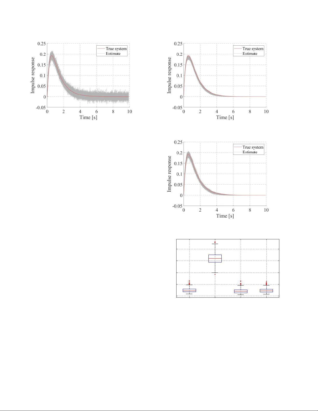
On the Coordinate Change to the First-Order Spline Kernel for Regularized Impulse Response Estimation

On the Coordinate Change to the First-Order Spline K er nel for Regularized Impulse Response Estimation ? Y usuke Fujimoto a and T ianshi Chen b a F aculty of En vir onmental Engineering, The University of Kitak yushu, W akamatsu-ku, Kitak yushu, 808-0135, Japan b School of Science and Engineering and Shenzhen Resear ch Institute of Big Data, The Chinese Univer sity of HongKong , Shenzhen, 518172, China Abstract The so-called tuned-correlated kernel (sometimes also called the first-order stable spline kernel) is one of the most widely used kernels for the regularized impulse response estimation. This kernel can be deri ved by applying an exponential decay function as a coordinate change to the first-order spline kernel. This paper focuses on this coordinate change and deri ves new kernels by inv estigating other coordinate changes induced by stable and strictly proper transfer functions. It is sho wn that the corresponding kernels inherit properties from these coordinate changes and the first-order spline kernel. In particular, they hav e the maximum entropy property and moreover , the inverse of their Gram matrices has sparse structure. In addition, the spectral analysis of some special kernels are provided. Finally , a numerical example is gi ven to sho w the e ffi cacy of the proposed kernel. K ey wor ds: Identification methods, kernel-based regularization methods, impulse response estimation, kernels. 1 INTR ODUCTION One of the main di ffi culties in system identification is to balance the data fit and the model complexity [1]. Recently , a new method to handle this issue is proposed by Pillonetto and De Nicolao, especially for the impulse response es- timation of linear time-inv ariant systems [2]. Their main idea comes from the regression over the Reproducing K er- nel Hilbert Space (RKHS) [3,4] in the machine learning field. These spacecs are related to biv ariate functions that are called kernels and this class of methods is often referred to as the kernel-based regularization methods. In contrast with the classical Prediction Error Methods (PEMs), a property of such methods is that it is possible to design through the kernel a model structure that contains a wide class of im- pulse responses. More specifically , recall that the classical PEMs first determines the model structure, and then tune its parameters according to the observed data. In this case, the set of all possible impulse responses is a finite dimensional manifold. On the other hand, the kernel-based regularization method, with a carefully designed kernel, searches the im- pulse response within a possibly infinite dimensional RKHS ? This paper was not presented at an y IF AC meeting. Correspond- ing author Y . Fujimoto. T el. + 81-93-695-3545. Email addr esses: y-fujimoto@kitakyu-u.ac.jp (Y usuke Fujimoto), tchen@cuhk.edu.cn (T ianshi Chen). and thus has the potential to model complex systems. One of the main issues for the kernel-based regularization method is how to design a suitable kernel. While various kernels hav e been proposed (e.g., [5,6,7]), three most widely used kernels are the so-called Stable Spline kernel (SS) [2], the T uned-Correlated kernel (sometimes also called the first- order stable spline kernel) [8], and the Diagonal-Correlated (DC) kernel [8]. These three kernels hav e simple structures and fa vorable properties, and their e ff ecti veness are shown in v arious works, e.g., [8,9,10,11]. Interestingly , these three kernels share some common prop- erties [7,12]. For e xample, they can be derived by apply- ing an exponential decay function as a coordinate change to di ff erent kinds of spline kernels [13] (cf. Section 2.2 for details). Moreover , the y also inherit some properties from the corresponding spline kernel [14], such as the maximum entropy (MaxEnt) property and the spectral analysis. Based on the abov e observations, the follo wing questions then arise naturally: • Instead of the exponential decay coordinate change, can we design kernels with other type of coordinate change suitable for system identification? • What is the corresponding a priori kno wledge embedded in such kernels? Preprint submitted to Automatica 20 December 2024 In this paper , we aim to address the above questions. In par- ticular , we will focus on the kernels deriv ed by applying the impulse response of a stable and strictly proper transfer function G ( s ) as the coordinate change function to the first- order spline k ernel, where s is the comple x frequenc y for the Laplace transform. Then it is obvious to see that the expo- nential decay function e − α t is a special case of the proposed kernels with G ( s ) = 1 s + α . Besides, in our preliminary work [15], we considered the case where the coordinate change is giv en by t n e − α t , which corresponds to G ( s ) = 1 ( s + α ) n . Here, we will consider more general cases and moreover , we will show that such coordinate change embeds a priori knowledge from G ( s ) on the re gularized impulse response, or equiv- alently , the corresponding RKHS inherits properties from G ( s ). For instance, the proposed kernels are always stable, and the estimated impulse response has the same con ver- gence rate as the coordinate change function. The relati ve degree of the impulse response is determined by the coor- dinate change function. More voer , we also sho w that the proposed kernels hav e the Maximum Entropy property and giv e the spectral analysis for some special cases based on the corresponding ones for the first-order spline kernel. The remaining part of this paper is or ganized as follo ws. Sec. 2 recaps the kernel-based regularization methods, and states the problem considered in this paper . Sec. 3 first shows the positi ve definiteness and stability of the proposed ker - nel. Then Sec. 4 shows properties of the proposed kernels related to zero-crossing. Sec. 5 discusses the Maximum En- tropy property of the proposed kernel, and Sec. 6 gi ves spec- tral analysis for some special cases. Sec. 7 sho ws a numer - ical example to demonstrate the e ff ectiv eness of coordinate changes. Finally Sec. 8 concludes this paper . [Notations] Sets of nonnegati ve real numbers and natural numbers are denoted by R 0 + and N , respecti vely . The n - dimensional identity matrix is denoted by I n . The in verse and the transposition of a matrix A are denoted by A − 1 and A > , respectiv ely . The determinant of a square matrix A is denoted by det( A ). k A k FR O denotes the Frobenius norm of matrix A . The ( i , j ) element of a matrix A is denoted by { A } i , j . When a is a vector , { a } i denotes the i th element of a . The Lebesgue integral of f ( x ) over X is denoted by R X f ( x ) d x , and the integral with the measure µ is denoted by R X f ( x ) d µ ( x ). In particular , the Lebesgue integral of f ( x ) over [ a , b ) is denoted by R b a f ( x ) d x . L 1 [0 , ∞ ] sho ws the set of absolute integrable functions o ver [0 , ∞ ), i.e., L 1 [0 , ∞ ] = { f | R ∞ 0 | f ( x ) | d x < ∞} . The set { a 1 , . . . , a n } is denoted by { a k } n k = 1 . The expected value and v ariance of random v ariables are denoted by E and V , respectiv ely . The limit lim t → + 0 f ( t ) denotes the right- sided limit at zero. Throughout the paper , s denotes the complex frequenc y for the Laplace transform, and e denotes the Napier’ s constant. 2 PR OBLEM SETTING 2.1 K ernel-based re gularization methods W e first recap the kernel-based regularized method for continuous-time systems. This paper focuses on single- input-single-output, bounded-input-bounded-output, stable, linear time in variant and causal systems described by y ( t ) = Z t 0 u ( t − τ ) g ( τ ) d τ + w ( t ) , (1) where t ∈ R 0 + is the time inde x, u ( t ) ∈ R , y ( t ) ∈ R , and w ( t ) ∈ R are the input, the measured output, and the mea- surement noise at time t , respectiv ely , g ( t ) : R 0 + → R is the impulse response of the system, and R t 0 u ( t − τ ) g ( τ ) d τ is the con volution of the input and the impulse response, w ( t ) is in- dependently and identically Gaussian distrib uted with mean 0 and variance σ 2 . The identification problem in this paper is to estimate g ( t ) from the measured output { y ( t k ) } N k = 1 and the input u ( t ) ov er the interval [0 , t N ], where t 1 , t 2 , . . . , t N are the sampling time instants. T o this end, we use the kernel-based regularization method where the estimated impulse response ˆ g ( t ) is given by ˆ g = argmin g ∈H N X k = 1 y ( t k ) − Z t k 0 u ( t k − τ ) g ( τ ) d τ ! 2 + γ k g k 2 H . (2) Here, H is a Hilbert space of functions g : R 0 + → R , and k · k H is the norm endowed to H , and γ > 0 is a regularization parameter . Clearly , a good estimate of the impulse response depends on a good choice of H . In the sequel, we assume that H is a Reproducing Kernel Hilbert Space (RKHS). The definitions of RKHS and the reproducing kernel are as follows. Let X be a nonempty set, and consider the Hilbert space of functions f : X → R denoted by H . Then H is a RKHS if ∀ x ∈ X , ∃ C x : | g ( x ) | ≤ C x k g k H , ∀ g ∈ H . (3) Further let h · , · i be the inner product endo wed to H . Then a symmetric bi variate function K : X × X → R is the repro- ducing kernel of H if it satisfies f ( x ) = h f , K ( x , · ) i , ∀ f ∈ H , (4) where K ( x , · ) indicates the single-v ariable function defined by setting the first argument of K to x . Reproducing kernels are also called kernels for short. It is well-known that the kernel K exists if the Hilbert space H is RKHS. W ith the abov e definitions, the optimal solution of (2) has explicit expression. Let K : R 0 + × R 0 + → R be the kernel of 2 H in (2). Also let O ∈ R N × N be a matrix which is defined as { O } i , j = Z t i 0 u ( t i − τ 1 ) Z t j 0 u ( t j − τ 2 ) K ( τ 1 , τ 2 ) d τ 1 d τ 2 . (5) Let y = [ y ( t 1 ) , . . . , y ( t N )] > ∈ R N and c ∈ R N be c = ( O + γ I N ) − 1 y . (6) Then, the optimal solution of (2) is gi ven by ˆ g ( t ) = N X i = 1 { c } i K u i ( t ) , (7) where K u i ( t ) is a function of t defined by K u i ( t ) = Z t i 0 u ( t i − τ ) K ( τ , t ) d τ . (8) See e.g., [9] for more details. 2.2 Pr oblem statement The Stable Spline (SS) kernel, the T uned-Correlated kernel (sometimes also called the first-order stable spline kernel), and the DC kernel can all be deri ved by applying an e x- ponential decay function as a coordinate change to di ff er - ent kinds of spline kernels. T o make this point clear, we let W ( · , · ) be a kernel function and X ( t ) be a coordinate change function. Then the aforementioned three kernels can all be put into the follo wing form K ( t 1 , t 2 ) = W ( X ( t 1 ) , X ( t 2 )) , t 1 , t 2 ∈ R 0 + . (9) Moreov er, the coordinate change functions X ( t ) are all e − α t : R 0 + → [0 , 1] for these three kernels, while the kernel W is the second order spline kernel for the SS kernel, the first order spline kernel for the TC kernel, and a generalized first order spline kernel for the DC kernel, cf. [16]. In particular , the TC kernel, K TC ( t 1 , t 2 ) = β min( e − α t 1 , e − α t 2 ) , t 1 , t 2 ∈ R 0 + (10) can be derived by applying e − α t : R 0 + → [0 , 1] as the coor- dinate change to the first-order spline kernel K S ( τ 1 , τ 2 ) = β min( τ 1 , τ 2 ) , τ 1 , τ 2 ∈ [0 , 1] , (11) where β > 0 and α > 0 are hyperparameters of the kernel. W e consider more general coordinate changes in this paper . Problem 1 Let G 0 ( s ) be a stable and strictly pr oper transfer function and g 0 ( t ) : R 0 + → R be the impulse r esponse of G 0 ( s ) . Her eafter , we consider pr operties of the kernel given by the first-or der spline kernel with | g 0 ( t ) | as the coor dinate change function, i.e., K G 0 ( τ 1 , τ 2 ) = min( | g 0 ( τ 1 ) | , | g 0 ( τ 2 ) | ) . (12) or equivalently the pr operties of the RKHS associated with K G 0 that is denoted by H G 0 below . 3 POSITIVE DEFINITENESS AND ST ABILITY W e first recall some definitions. A kernel K : X × X → R is said to be positive definite if the Gram matrix of K defined as                         K ( x 1 , x 1 ) K ( x 1 , x 2 ) · · · K ( x 1 , x m ) K ( x 2 , x 1 ) K ( x 2 , x m ) . . . . . . . . . K ( x m , x 1 ) K ( x m , x 2 ) · · · K ( x m , x m )                         ∈ R m × m , (13) is positi ve semidefinite for any [ x 1 , . . . , x m ] > ∈ X m and for any m ∈ N . The Moore-Aronszajin theorem states that if K is positi ve definite, then there exists a unique RKHS whose reproducing kernel is K [3]. A kernel K : R 0 + × R 0 + → R is said to be stable if H , the RKHS associated with K , satisfies H ⊂ L 1 [0 , ∞ ]. Then we hav e the following result 1 . Theorem 2 The kernel (12) is positive definite and mor e- over , stable, i.e., the corr esponding RKHS H G 0 is a subspace of L 1 [0 , ∞ ] . Theorem 2 shows that the kernel (12) is a positive semidef- inite kernel and moreo ver , for any g ∈ H G 0 , g ∈ L 1 [0 , ∞ ]. 4 ZER O-CROSSING RELA TED PROPER TIES The follo wing proposition shows that if g 0 ( t ) has a zero- crossing, then any g ∈ H G 0 inherits this zero-crossing. Proposition 3 Assume that g 0 ( t ) satisfies g 0 ( τ ) = 0 for some τ ∈ R 0 + . Then, g ( τ ) = 0 for any g ∈ H G 0 . This proposition suggests that, if one kno ws that the true impulse response is zero at some time instant τ , then one should design G 0 ( s ) such that g 0 ( τ ) = 0. A typical case is τ = 0, i.e., the relativ e degree of the system is known to be higher than or equal to two. For this case, the result can be further strengthened and is sho wn in the following theorem. 1 All proofs of propositions are deferred to the Appendix. 3 Theorem 4 Assume that the identification input u ( t ) is k − 1 times di ff er entiable, and satisfies       d i u d t i       < ∞ , i = 0 , 1 , . . . , k − 1 . (14) If g 0 ( t ) satisfies lim t → + 0 d j dt j g 0 ( t ) = 0 for j = 0 , 1 , . . . , k , then lim t → + 0 d j dt j ˆ g ( t ) = 0 for j = 0 , 1 , . . . , k . Moreov er, for any g ∈ H G 0 , ho w fast g ( t ) con verges to 0 also depends on g 0 ( t ), which is stated in the following theorem. Theorem 5 Assume that the input u ( t ) is bounded, and let U ∈ R N be a vector whose i-th element is R t i 0 u ( t i − τ ) d τ . When G 0 ( s ) is stable and G 0 ( s ) , 0 , ˆ g ( t ) | g 0 ( t ) | con ver ges to U > c when t → ∞ , where c is defined as (6). In summary , H G 0 inherits some properties of g 0 , i.e., how g 0 crosses or con verges to zero. This is because the linear spline kernel in (12) is emplo yed. More specifically , let H S be the RKHS associated with the first order spline kernel (11). Noting that f (0) = 0 for any f ∈ H S from the reproducing property , the properties of H G 0 giv en in this section can be deriv ed accordingly . 5 MAXIMUM ENTR OPY PROPER TY Interestingly , the kernel (12) also inherits the maximum en- tropy property of the linear spline kernel (11). Theorem 6 F or a given g 0 ( t ) with t 0 , . . . , t n be a sequence fr om R 0 + ∪ {∞} , let T 0 , . . . , T n be the permutation of { t 0 , . . . , t n } such that 0 = | g 0 ( T 0 ) | < | g 0 ( T 1 ) | < · · · < | g 0 ( T n ) | , (15) and consider the stochastic pr ocess defined by h o ( T k ) = k X j = 1 w ( j ) q | g 0 ( T j ) | − | g 0 ( T j − 1 ) | , k = 1 , . . . , n , h ( T 0 ) = 0 , (16) wher e w ( k ) is a white Gaussian noise with unit variance. Then, h o ( T k ) is a Gaussian pr ocess with zer o mean and K G 0 ( T i , T j ) as its covariance function. In addition, let h ( T ) be any stochastic pr ocess defined over { T 0 , . . . , T n } with h ( T 0 ) = 0 . Then, the Gaussian process h o is the solution of the MaxEnt pr oblem max h ( · ) H ( h ( T 0 ) , . . . , h ( T n )) subject to E ( h ( T i )) = 0 , i = 1 , . . . , n , V ( h ( T i ) − h ( T i − 1 )) = | g 0 ( T i ) | − | g 0 ( T i − 1 ) | . wher e H ( h ( T 0 ) , . . . , h ( T n )) denotes the di ff erential entr opy of [ h ( T 0 ) , . . . , h ( T n )] > 2 . This Maximum Entropy interpretation also suggests the spe- cial structure of the in verse of the Gram matrix of K G 0 . For a given g 0 ( t ) with t 0 , . . . , t n be a sequence from R 0 + ∪ {∞} , let T 0 , . . . , T n be a permutation of t 0 , . . . , t n , which satisfies (15). Also let ¯ K ∈ R ( n + 1) × ( n + 1) be a Gram matrix of K G 0 de- fined as ¯ K =                 K G 0 ( t 0 , t 0 ) · · · K G 0 ( t 0 , t n ) . . . . . . . . . K G 0 ( t n , t 0 ) · · · K G 0 ( t n , t n )                 . (17) Since | g 0 ( T 0 ) | is assumed to be zero, ¯ K has a ro w and a column whose all elements are zero. W e define K ∈ R n × n as a matrix constructed by removing such a row and column from ¯ K . Note that K is also a Gram matrix of K G 0 . Before showing the structure of K − 1 , we first gi ve the follo wing result. Theorem 7 The determinant of K is given as det ( K ) = | g 0 ( T 1 ) | Π n − 1 i = 1 ( | g 0 ( T i + 1 ) | − | g 0 ( T i ) | ) . (18) Theorem 7 gi ves the condition where the in verse of K exists; g 0 ( t i ) , 0 for all i and | g 0 ( t i ) | , | g 0 ( t j ) | for all i , j . Theorem 8 Let ¯ g = [ | g 0 ( t 0 ) | , . . . , | g 0 ( t n ) | ] > ∈ R n + 1 , and also let g ∈ R n be a vector which r emoves the element corr e- sponds to | g 0 ( T 0 ) | fr om ¯ g. Let R ∈ R n × n be a row-permutation matrix such that Rg =                 | g 0 ( T 1 ) | . . . | g 0 ( T n ) |                 ,                 g 1 . . . g n                 . (19) Then the in verse matrix of K is given as K − 1 = R > PR , (20) wher e P ∈ R n × n is the in verse matrix of the Gram matrix of the first-or der spline kernel [14], { P } i , j =                        g 2 g 1 ( g 2 − g 1 ) i = j = 1 , g i + 1 − g i − 1 ( g i + 1 − g i )( g i − g i − 1 ) i = j = 2 , . . . , n − 1 . 1 g n − g n − 1 i = j = n , 0 | i − j | > 1 , − 1 max( g i , g j ) − min( g i , g j ) otherwise , (21) 2 The di ff erential entropy of random v ariable x is defined by − R p ( x ) log p ( x ) d x , where the integral is taken over the support of p ( x ). 4 0 10 20 30 40 0 10 20 30 40 (a) Sparsity pattern of K − 1 0 10 20 30 40 0 10 20 30 40 (b) Sparsity pattern of P Fig. 1. Sparsity pattern of matrices Theorem 8 gi ves the explicit form of the in verse matrix of K . Note that P is a tri-diagonal matrix. This theorem indicates that K − 1 has a sparse structure, i.e., it has at most three elements in each ro w (or column). Example 1 F or illustr ation, we consider the case g 0 ( t ) = te − t , or equivalently , G 0 ( s ) = 1 ( s + 1) 2 , and show that the cor- r esponding K − 1 has a sparse structur e. W e set t i = 0 . 1 × i ( i = 1 , . . . , 40) , and computed K − 1 accor ding to Theor em 8. F igs. 1a and 1b show the sparsity patterns of K − 1 and P, r e- spectively , by using the matlab command spy . The horizon- tal and vertical axes show the column and r ow of each ma- trix, respectively , and the dots show the non-zer o elements. W e can see that P is tri-diagonal, and K − 1 has at most thr ee non-zer o elements in each r ow or column. The sparsity pat- tern may not be seen in a numerically computed K − 1 , e .g., the one computed by using matlab command inv . F or in- stance, spy(inv( K )) shows that all elements in inv( K ) ar e non-zer o. T o illustr ate the e ff ectiveness of Theor em 8, we compute     2 × I 100 − K  K − 1  0 −  K − 1  0 K     FR O , wher e  K − 1  0 shows a numerically computed in verse of K with Theor em 8 or inv . Then we have 1 . 4 × 10 − 12 with Theor em 8 and 1 . 6 × 10 − 12 with inv , r espectively . 6 SPECTRAL ANAL YSIS OF MUL TIPLE POLE SPLINE KERNEL It is well-kno wn from Mercer’ s Theorem that under suitable assumptions on the kernel an y function in the RKHS can be represented by an orthonormal series. W e sho w such an orthonormal basis for H G 0 , which can yield a reasonable finite dimensional approximation of H G 0 and can make some computations easy and f ast. In this section, we focus on (12) where G 0 ( s ) = 1 ( s + α ) n + 1 with n = 1 , 2 , . . . , and show the spectral analysis of (12). This kernel is proposed in [15] and called the Multiple pole Spline kernel. 6.1 Pr eliminary W e first introduce some definitions for a positive semidefi- nite kernel K : X × X → R with a compact set X . Let µ be a nondegenerate Borel measure on X . Also let L 2 ( X , µ ) denote the space of functions of f : X → R such that R X | f ( x ) | 2 d µ ( x ) < + ∞ . F or a giv en kernel K and φ ∈ L 2 ( X , µ ), we define an integral operator on L 2 ( X , µ ): L K φ ( x ) = Z X K ( x , x 0 ) φ ( x 0 ) d µ ( x 0 ) , x ∈ X . (22) If for some λ , L K φ ( x ) = λφ ( x ) , x ∈ X , (23) has the solution other than φ ( x ) = 0, λ and the solution are called the eigenv alues and eigenfunctions of L K , respec- tiv ely . T wo distinct eigenfunctions φ ( x ) and ψ ( x ) are orthog- onal, i.e., h φ, ψ i L 2 ( X ,µ ) = 0. Then, the kernel K has a series expansion K ( x , x 0 ) = ∞ X i = 1 λ i φ i ( x ) φ i ( x 0 ) , (24) which con ver ges uniformly and absolutely on X × X . Consider the first-order spline kernel K S ( x , x 0 ) = min( x , x 0 ) : [0 , 1] × [0 , 1] → R with µ being the Lebesgue measure. In this case, the eigen values and eigenfunctions are given by λ i = 1  i − 1 2  2 π 2 , φ i ( x ) = √ 2 sin i − 1 2 ! π x ! , (25) Z 1 0 min( x , x 0 ) φ i ( x 0 ) d x 0 = λ i φ i ( x ) ( i = 1 , 2 , . . . ) . (26) W ith these λ i and φ i , the spline k ernel has the series expan- sion (24). 6.2 Main r esult W e consider the case G 0 ( s ) = κ ( s + α ) n + 1 , n = 1 , 2 , . . . , i.e., K G 0 ( τ 1 , τ 2 ) = min  τ n 1 e − ατ 1 , τ n 2 e − ατ 2  . (27) For the simplicity of notations and discussions, we take κ = 1 in the following. The extension to other κ ∈ R is straightfor- ward. In the rest of this section, λ i and φ i denote the values and functions defined in (25). Before sho wing the main result, we first show a lemma. Lemma 9 Let T > 0 , and x ∈ [0 , T ] . Then, λ i and φ i defined by (25) satisfy Z T 0 min( x , x 0 ) φ i ( x 0 / T ) d x 0 = T 2 λ i φ i ( x / T ) . (28) In addition, Z T 0 φ i ( x 0 / T ) φ j ( x 0 / T ) d x 0 = ( 0 i , j , T i = j . (29) 5 Lemma 9 gi ves the eigen values and eigenfunctions of min( x , x 0 ) over ( x , x 0 ) ∈ [0 , T ] × [0 , T ] for T > 0. In partic- ular , 1 √ T φ i ( x 0 / T ) are orthonormal eigenfunctions. The main result of this section is stated as follo ws. Theorem 10 Let m : R 0 + → R 0 + be a function defined by m ( τ ) =        1 2 τ n e − ατ 0 ≤ τ ≤ n α  n α  n e − n − 1 2 τ n e − ατ τ ≥ n α , (30) and consider the measure induced by m; d m = dm d τ d τ with the Lebesgue measur e d τ . Also let λ n , i and φ n , i be λ n , i =  n α e  2 n λ i , φ n , i ( τ ) =  ae n  n 2 φ i  τ n e − ατ  α e n  n  . (31) Then, we have Z ∞ 0 min( τ n 1 e − ατ 1 , τ n 2 e − ατ 2 ) φ n , i ( τ 2 ) d m ( τ 2 ) = λ n , i φ n , i ( τ 1 ) , (32) with Z ∞ 0 φ n , i ( τ ) φ n , j ( τ ) d m ( τ ) = ( 1 i = j , 0 i , j . (33) Theorem 10 suggests that λ n , i and φ n , i are the eigen values and eigenfunctions of K G 0 with the measure induced by d m , respectiv ely . Based on Theorem 10, we hav e the following theorem. Theorem 11 Let G 0 ( s ) = 1 ( s + α ) n + 1 . (1) the series expansion K G 0 ( τ 1 , τ 2 ) = ∞ X i = 1 λ n , i φ n , i ( τ 1 ) φ n , i ( τ 2 ) , (34) con ver ges uniformly and absolutely on R 0 + × R 0 + . (2) n p λ n , i φ n , i o ∞ i = 1 forms an orthonormal basis of H G 0 , and H G 0 has an equivalent r epr esentation; H G 0 = { f | f ( τ ) = ∞ X i = 1 f i φ n , i ( τ ) , ∞ X i = 1 f 2 i λ n , i < ∞} . (35) Mor eover , the norm of f is given by k f k 2 H G 0 = ∞ X i = 1 f 2 i λ n , i . (36) 0 0 5 10 15 0.1 0.2 0.3 0.4 Fig. 2. Illustration of m ( τ ) with n = 1 , α = 1 0 0 5 10 15 0.1 0.2 0.3 0.4 0.5 Fig. 3. Illustration of dm d τ with n = 1 , α = 1 0 5 10 15 0 0 0 2 2 2 -2 -2 1 1 Fig. 4. Illustration of φ n , i ( τ ) with n = 1 , α = 1 Example 2 F or illustration, we show the case with n = 1 and α = 1 . F igs. 2 and 3 shows m ( τ ) defined by (30) and dm d τ , r espectively . The horizontal axes show τ , and the vertical axes show m ( τ ) and dm d τ , r espectively . In this case , n α = 1 and dm d τ = 0 at τ = 1 . F ig. 4 shows φ 1 , i ( τ ) for i = 1 , 2 , 3 . The horizontal axes show τ , and the vertical axes show φ 1 , i ( τ ) . The top, middle, and bottom figur es show φ 1 , 1 ( τ ) , φ 1 , 2 ( τ ) , and φ 1 , 3 ( τ ) . These eigenfunctions satisfy φ n , i (0) = 0 and lim τ →∞ φ n , i ( τ ) = 0 as we expected. 6 Fig. 5. Illustration of k K − K M k FRO W ith the same n and α , we also compute k K − K M k FR O wher e ( i , j ) elements of K and K M ar e given as K G 0 ( t i , t j ) and P M ` = 1 λ n ,` φ n ,` ( t i ) φ n ,` ( t j ) , r espectively , with t i = 0 . 1 × i ( i = 1 , . . . , 40) . F ig. 5 illustrates how k K − K M k FR O con ver ges to zer o with incr easing M . The horizontal and vertical axes show M and k K − K M k FR O , r espectively . 7 ILLUSTRA TIVE EXAMPLE In Sec. 7, we gi ve a numerical example to illustrate the e ff ectiv eness of the proposed kernel. The target system is giv en by G ∗ ( s ) = 1 ( s + 1)( s + 3) , (37) hence the relativ e degree of the target is two. For G 0 ( s ), we employ G 0 ( s ) = θ 3 ( θ 1 − θ 2 ) ( s + θ 1 )( s + θ 2 ) = θ 3 1 s + θ 2 − 1 s + θ 1 ! , (38) with θ = [ θ 1 , θ 2 , θ 3 ] > ∈ R 3 as the hyperparameters of the kernel. The impulse response of G 0 ( s ) is g 0 ( t ) = θ 3 ( e − θ 2 t − e − θ 1 t ) , (39) thus g 0 (0) = 0 for any θ . As sho wn in Sec. 4, this makes the estimated impulse response ˆ g (0) = 0. This means that we enjoy a priori knowledge on the system that its relati ve degree is higher or equal to tw o. W e consider the case where the input is the impulsive input, and the noise v ariance σ 2 = 10 − 4 . The sampling period T s is set to 0.1 [s], and we collect { y ( T s ) , y (2 T s ) , . . . , y (100 T s ) } = { y ( kT s ) } 100 k = 1 . Fig. 6 shows an example of such observed data { y ( kT s ) } 100 k = 1 . The horizontal axis shows time, and the vertical axis shows the observed output. Each dot shows the observed data ( iT s , y ( iT s )). In the follo wing, we identify the impulse 02468 10 -0.05 0 0.05 0.1 0.15 0.2 0.25 T ime [s] Output Fig. 6. Illustration of observed data Fig. 7. Estimated impulse responses with K G 0 response from such data for 300 times with independent noise realizations. W e employ the Empirical Bayes method to tune the hyper - parameters, i.e., θ is tuned so as to maximize −  log det  O + σ 2 I N  + y >  O + σ 2 I N  − 1 y  , (40) where γ is set to σ 2 . Note that O depends on the hyperparam- eter θ . This is based on the Gaussian process interpretation of the kernel based regularization methods. In this interpre- tation, the kernel is regarded as the cov ariance function of the zero-mean Gaussian process, and (40) shows the loga- rithm of marginal likelihood (some constants are ignored). Such a tuning is called the Empirical Bayes [9]. Using G 0 ( s ) defined by (38) and the Empirical Bayes method, we perform the identification with K G 0 for 300 times with independent noise realizations. Fig. 7 shows the estimated and true impulse response of the target system. The horizontal axis sho ws time, and the vertical axis sho ws the impulse response. The gray lines are 300 estimated impulse responses, and the red line shows the true impulse response. Apparently , the behavior of the original impulse response is well approximated with K G 0 . 7 Fig. 8. Estimated impulse responses with TC k ernel (Empirical Bayes) For comparison, we also show the result with the TC ker- nel and the Empirical Bayes. Recall that the TC k ernel is defined as (10). Fig. 8 shows the 100 estimated impulse re- sponses with the TC kernel and the Empirical Bayes. The estimated impulse responses conv erge to zero slowly , and show overfitting beha vior . For comparison, we also show the results with oracle hyper - parameters, i.e., hyperparameters tuned with the true impulse response. Let ˆ g = [ ˆ g ( T s ) , ˆ g (2 T s ) , . . . , ˆ g (100 T s )] > ∈ R 100 and g ∗ = [ g ∗ ( T s ) , g ∗ (2 T s ) , . . . , g ∗ (100 T s )] > ∈ R 100 . Noting that we consider the case with impulsi ve input, we hav e ˆ g = K  K + σ 2 I 100  − 1 ( g ∗ + w ) =  I 100 − σ 2  K + σ 2 I 100  − 1  ( g ∗ + w ) , (41) where K ∈ R 100 × 100 is a Gram matrix of the k ernel with t i = iT s and w = [ w ( T s ) , w (2 T s ) , . . . , w (100 T s )] > ∈ R 100 . Then, ˆ g − g ∗ = − σ 2  K + σ 2 I 100  − 1 g ∗ +  I 100 − σ 2  K + σ 2 I 100  − 1  w , (42) and the mean square error on the sampled instants t i = iT s ( i = 1 , . . . , 100) becomes E h ( ˆ g − g ∗ ) > ( ˆ g − g ∗ ) i = σ 4 ( g ∗ ) >  K + σ 2 I 100  − 2 g ∗ + 100 σ 2 + σ 6 T r  ( K + σ I 100 ) − 2  − 2 σ 4 T r  ( K + σ I 100 ) − 1  . (43) In the following, we show the results with hyperparameters which minimize (43). Figs. 9 and 10 show the 300 estimated impulse responses with such hyperparameters. Figs. 9 and 10 employ the pro- Fig. 9. Estimated impulse response with K G 0 (oracle) Fig. 10. Estimated impulse responses with TC kernel (Oracle) Proposed (EB) SS-1 (EB) Proposed (oracle) SS-1 (oracle) 0 0.04 0.08 0.12 0.16 Square errors Fig. 11. Boxplots of square errors on sampled instants posed and TC kernel, respectiv ely . In this case, the esti- mated impulse response with the TC kernel con ver ges to zero smoothly . Fig. 11 shows the boxplots of the square errors on the sam- pled instants, i.e., ( ˆ g − g ) > ( ˆ g − g ), with 300 independent noise realizations. The left two boxes sho w the results with the Empirical Bayes, and the right two boxes sho w the results with the hyperparameter tuned according to the mean square 8 error on the sampled instants. The proposed kernel with the Empirical Bayes shows almost the same performance as the TC with the oracle hyperparameter, and the proposed ker - nel with the oracle hyperparameter outperforms the others. These results sho w that the proposed kernel is more appro- priate for G ∗ ( s ) than the TC kernel. As a statistical analysis, we perform the W ilcoxon rank sum tests for two cases. In the first case, we focus on the proposed kernel with the Empirical Bayes and the TC kernel with the oracle hyperparameter . The null hypothesis is that two medians of the square errors on the sampled instants are the same (two-sided rank sum test). The p -v alue is 0.37, thus this null hypothesis can not be rejected. This implies that the proposed method with the Empirical Bayes performs as well as the TC kernel with the optimal hyperparameter . In the second case, we focus on the proposed and the TC kernel with the oracle hyperparameters. The null hypothesis is that the median of the square errors become smaller with the TC kernel (one-sided rank sum test). The p -value is 2 . 0 × 10 − 4 , thus the alternati ve hypothesis is highly significant. This suggests that the proposed kernel has potential to achie ve better estimate than the TC kernel. From the abov e results, it is confirmed that the prposed kernel (12) can be useful for regularized impulse resopnse estimation, provided that the coordinate change is designed by taking into account the a priori knowledge on the system to be identified. 8 CONCLUSION This paper focuses on kernels deri ved by appling coordinate changes induced by stable and strictly proper transfer func- tions to the first-order spline kernel. The y are generaliza- tions of the tuned-correlated kernel, which is one of the most widely used kernels in the regularized impulse response esti- mation. It is shown that the proposed kernels inherit proper- ties from the coordinate changes such as the relati ve de gree and the con vergence rate. Also they inherit the Maximum Entropy property from the first-order spline kernel. Spectral analysis is giv en for the case where the coordinate change is chosen as t n e − α t . Numerical le xample is giv en to demon- strate the e ff ectiveness of the proposed kernel and shows that a suitable coordinate change could gi ve better performance than the tuned-correlated kernel. Extension to cases for the second-order spline kernel or the generalized spline kernel are future tasks. Another future task is to find the optimal coordinate change in some sense for gi ven a priori knowledge on the system to be identified. References [1] L. Ljung. System Identification: Theory for the User . Prentice Hall, Upper Saddle Riv er, NJ, 2nd edition edition, 1999. [2] G. Pillonetto and G. De Nicolao. A new k ernel-based approach for linear system identification. Automatica , 46(1):81–93, 2010. [3] N. Aronszajn. Theory of Reproducing Kernels. T ransactions of the American Mathematical Sociery , 68(3):337–404, 1950. [4] B. Sch ¨ olkopf and A. J. Smola. Learning with K ernels: Support V ector Machines, Regularization, Optimization, and Beyond . MIT press, 2001. [5] G. Prando and A. Chiuso. Model reduction for linear Bayesian System Identification. In Pr oceedings of IEEE 54th Conference on Decision and Contr ol , pages 2121–2126, 2015. [6] T . Chen and L. Ljung. Regularized system identification using orthonormal basis functions. In Pr oceedings of 2015 European Contr ol Conference , pages 1291–1296. IEEE, 2015. [7] T . Chen. On k ernel design for regularized L TI system identification. Automatica , 90:109–122, 2018. [8] T . Chen, H. Ohlsson, and L. Ljung. On the estimation of transfer functions, re gularizations and Gaussian processes–Revisited. Automatica , 48(8):1525–1535, 2012. [9] G. Pillonetto, F . Dinuzzo, T . Chen, G. De Nicolao, and L. Ljung. Kernel methods in system identification, machine learning and function estimation: A surve y . A utomatica , 50(3):657–682, 2014. [10] G. Bottegal, G. Pillonetto, and H. Hjalmarsson. Bayesian Kernel- Based System Identification with Quantized Output Data. In Pr oceedings of 17th IF A C Symposium on System Identification , 2015. [11] G. Prando, D. Romeres, G. Pillonetto, and A. Chiuo. Classical vs. Bayesian methods for linear system identification: point estimators and confidence sets. In Pr oceedings of 2016 European Contr ol Confer ence , pages 1365–1370, 2016. [12] T . Chen. Continuous-Time DC Kernel — A Stable Generalized First-Order Spline Kernel. Tr ansactions on Automatic Contr ol , 2018. [13] G. W ahba. Spline Models for Observational Data . SIAM, 1990. [14] T . Chen, T . Ardeshiri, F . P . Carli, A. Chiuso, L. Ljung, and G. Pillonetto. Maximum entropy properties of discrete-time first- order stable spline kernel. Automatica , 66:34–38, 2016. [15] Y . Fujimoto, I. Maruta, and T . Sugie. Extension of first-order stable spline kernel to encode relativ e degree. In Pr oceedings of 20th IF AC W orld Congr ess , pages 15481–15486, 2017. [16] T . Chen, G. Pillonetto, A. Chuso, and L. Ljung. Continuous-time dc kernel – a stable generalized first order spline kernel. In Pr oceedings of IEEE 55 th Conference on Decision and Control , pages 4647– 4652, 2016. [17] F . Cucker and S. Smale. On the mathematical foundations of learning. Bulletin of the American mathematical society , 39(1):1–49, 2001. [18] R. M. Corless, G. H. Gonnet, D. E. G. Hare, D. J. Je ff rey , and D. E. Knuth. On the Lambert W function. Advances in Computational mathematics , 5(1):329–359, 1996. A Proofs A.1 Pr oof of Theor em 2 K G 0 is interpreted as the first-order spline kernel with β = max t | g 0 ( t ) | and the coordinate change | g 0 ( t ) | max t | g 0 ( t ) | : R 0 + → [0 , 1]. This suggests that K G 0 is positi ve definite, hence there exists an RKHS associated with K G 0 . W e recall the following proposition for the proof about the stability; if the kernel K is a nonnegati ve valued function, i.e., K : R 0 + × R 0 + → R 0 + , then K is stable if and only if " R 2 0 + K ( τ 1 , τ 2 ) d τ 1 d τ 2 < ∞ . (A.1) 9 See Proposition 15 in [9] for more detail about the stability of the kernel. The proof about the stability is based on the follo wing Lemma. Lemma 12 F or any stable and strictly pr oper rational transfer function G 0 ( s ) , ther e e xists β ∗ > 0 and α ∗ > 0 which satisfies | g 0 ( t ) | ≤ β ∗ e − α ∗ t ∀ t ∈ R 0 + . (A.2) The proof of Lemma 12 is gi ven in Appendix A.2. Based on Lemma 12, " R 2 0 + K G 0 ( τ 1 , τ 2 ) d τ 1 d τ 2 ≤ " R 2 0 + β ∗ min( e − α ∗ τ 1 , e − α ∗ τ 2 ) d τ 1 d τ 2 = 2 β ∗ α 2 ∗ < ∞ . (A.3) Since K G 0 is a nonne gativ e valued kernel and satisfies (A.1), the statement is prov en. A.2 Pr oof of Lemma 12 From the assumption that G 0 ( s ) is stable and a strictly proper rational function of s , g 0 ( t ) is divided into four parts; derived from single-real poles, single-complex poles, repeated real poles, and repeated complex poles. In summary , we ha ve g 0 ( t ) = N real X i = 1 M real − 1 X j = 0 A i , j t j e − α real t + N comp X i = 1 M comp − 1 X j = 0 t j e − α comp i t ( B i , j sin ω i t + C i , j cos ω i t ) , (A.4) where N real , N comp , M real , and M comp denote the number of distinct real poles, the number of distinct comple x poles, the largest multiplicity of the real poles, and the largest multi- plicity of the complex poles, respecti vely . − α real i ∈ R , ( i = 1 , . . . , N real ) and and − α comp i ± ω i i , ( i = 1 , . . . , N comp ) show the distinct real poles and complex poles, respecti vely . Note that α real i > 0 and α comp i > 0 from the stability assumption. In the following, we show that each term of (A.4) is bounded by an exponential. For the ease notations, we employ α instead of α real i for a while. W e sho w that t j e − α t ( i ≥ 1) is bounded by j !  2 α  j e − α 2 t , where j ! denotes the factorial of j , i.e., j ! = j × ( j − 1) × ( j − 2) × · · · × 2 × 1. For ∀ t ∈ R 0 + , j ! 2 α ! j e − α 2 t − t j e − α t = j ! 2 α ! j e − α t e α 2 t − 1 j !  α 2  j t j ! = j ! 2 α ! j e − α t X k ≥ 0 , k , j 1 k !  α 2 t  k ≥ 0 , (A.5) holds. The second equality is deri ved from the T aylor ex- pansion of the exponential function, and the last inequality is deri ved from α > 0 , e − α t > 0 and t ≥ 0. From this inequal- ity , we have         N real X i = 1 M real − 1 X j = 0 A i , j t j e − α real i t         ≤ N real X i = 1 M real − 1 X j = 0    A i , j        t j e − α real i t     ≤ N real X i = 1 M real − 1 X j = 0    A i , j    c i , j ∗ e − 1 2 α real i t , (A.6) where c i , j ∗ = j !  2 α real i  j . Let α real ∗ = min i ( 1 2 α real i ). Then, e − 1 2 α real i t ≤ e − α real ∗ t for t ∈ R 0 + and we hav e         N real X i = 1 M real − 1 X j = 0 A i , j t j e − α real i t         ≤         N real X i = 1 M real − 1 X j = 0    A i , j    c i , j ∗         e − α real ∗ t ≤ β real ∗ e − α real ∗ t , (A.7) with β real ∗ = N real X i = 1 M real − 1 X j = 0    A i , j    c i , j ∗ . (A.8) By noting    ( B i , j sin ω i t + C i , j cos ω i t )    ≤ q B 2 i , j + C 2 i , j , (A.9) the same proof can be applied for the second term of (A.4), and         N comp X i = 1 M comp − 1 X j = 0 t j e − α comp i t ( B i , j sin ω i t + C i , j cos ω i t )         ≤ β comp ∗ e − α comp ∗ t , (A.10) with α comp ∗ = min i 1 2 α comp i , β comp ∗ = N comp X i = 1 M comp − 1 X j = 0 q B 2 i , j + C 2 i , j j !       2 α comp i       j . (A.11) 10 From the abov e discussions, we have | g 0 ( t ) | ≤ β real ∗ e − α real ∗ t + β comp ∗ e − α comp ∗ t ≤ β ∗ e − α ∗ t , (A.12) where β ∗ = 2 max  β real ∗ , β comp ∗  , α ∗ = min  α real ∗ , α comp ∗  , (A.13) and this completes the proof. A.3 Pr oof of Pr oposition 3 From the reproducing property of K G 0 , g ( τ ) =  g , K G 0 ( τ , · )  = h g , 0 i = 0 . (A.14) Here we use K G 0 ( τ , t ) = min(0 , | g 0 ( t ) | ) = 0. A.4 Pr oof of Theor em 4 W e first pro ve the case where k = 0. Consider K u i ( t ) defined by (8). From the assumption that g 0 ( t ) → 0 when t → + 0, K u i ( t ) is rewritten as K u i ( t ) = Z t 0 u ( t i − τ ) g 0 ( τ ) d τ + Z t i t u ( t i − τ ) g 0 ( t ) d τ , (A.15) for su ffi ciently small t . By noting | R t i 0 u ( t i − τ ) d τ | < ∞ , we hav e lim t → + 0 K u i ( t ) = 0 from    K u i ( t )    ≤       Z t 0 u ( t i − τ ) g 0 ( τ ) d τ       + | g 0 ( t ) |       Z t i t u ( t i − τ ) d τ       . (A.16) This holds for all i , and we conclude lim t → 0 ˆ g ( t ) → 0. Next, we consider the case k = 1. From (A.15), we have d d t K u i ( t ) = d g 0 d t Z t i t u ( t i − τ ) d τ . (A.17) Again by noting that u ( t ) is bounded and dg 0 dt → 0 from the assumption, we hav e lim t → + 0 d dt K u i = 0 and d ˆ g dt → 0. Finally , we prov e the case where k ≥ 2. Let U i ( t ) = R t i t u ( t i − τ ) d τ . When k ≥ 2, we have d k d t k K u i ( t ) = k X j = 0 d j g 0 d t j d k − j U i d t k − j . (A.18) From the assumption that u ( t ) and its deriv ativ es are bounded, the deriv ati ves of U i ( t ) are also bounded for j = 0 , 1 , . . . , k . Thus, if d j g 0 dt j → 0 for all j = 0 , . . . , k , we hav e lim t → + 0 d k dt k K u i ( t ) = 0 and the proof has been completed. A.5 Pr oof of Theor em 5 Consider K u i ( t ) defined by (8). Let T 1 , i ( t ) ⊂ [0 , t i ] and T 2 , i ( t ) ⊂ [0 , t i ] be sets defined by T 1 , i ( t ) = { τ | | g 0 ( t ) | ≤ | g 0 ( τ ) | , 0 ≤ τ ≤ t i } and T 2 , i ( t ) = { τ | | g 0 ( t ) | ≥ | g 0 ( τ ) | , 0 ≤ τ ≤ t i } . This indicates that K G 0 ( t , τ ) = | g 0 ( t ) | when τ ∈ T 1 , i ( t ) and K G 0 ( t , τ ) = | g 0 ( τ ) | when τ ∈ T 2 , i ( t ). Hence, we have K u i ( t ) | g 0 ( t ) | = Z T 1 , i ( t ) u ( t i − τ ) d τ + Z T 2 , i ( t ) u ( t i − τ )      g 0 ( τ ) g 0 ( t )      d τ . (A.19) Note that 0 ≤     g ( τ ) g ( t )     ≤ 1 when τ ∈ T 2 , i ( t ). Since the integrand of the second term is bounded and the Lebesgue measure of T 2 , i ( t ) goes to zero when t → ∞ (because g 0 ( t ) → 0), lim t →∞ K u i ( t ) | g 0 ( t ) | = Z t i 0 u ( t i − τ ) d τ , (A.20) and this indicates lim t →∞ ˆ g ( t ) | g 0 ( t ) | = U > c . (A.21) A.6 Pr oof of Theor em 2 The former half of the theorem is easily confirmed by the direct calculation; E [ h o ( T i ) h o ( T j )] = min( i , j ) X ` = 1 | g 0 ( T ` ) | − | g 0 ( T ` − 1 ) | = | g 0 ( T min( i , j ) ) | , (A.22) and by noting | g 0 ( T min( i , j ) ) | = min( | g 0 ( T i ) | , | g 0 ( T j ) | ), K G 0 is the cov ariance function of h o ( T k ). The latter half of the theorem is based on the Lemma 1 of [14], which is stated as follo ws. Lemma 13 (Chen et al .) Let h ( t ) be any stoc hastic pr ocess with h ( t 0 ) = 0 for t 0 = 0 . F or any n ∈ N and 0 = t 0 ≤ t 1 ≤ · · · ≤ t n , the discr ete-time W iener pr ocess is the solution of the MaxEnt pr oblem max h ( · ) H ( h ( t 0 ) , . . . , h ( t n )) subject to E ( h ( t i )) = 0 , i = 1 , . . . , n , V ( h ( t i ) − h ( t i − 1 )) = c ( t i − t i − 1 ) , 11 wher e the discr ete-time W iener pr ocess is given by h W ( t 0 ) = 0 , t 0 = 0 , h W ( t k ) = k X i = 1 w ( i − 1) √ t i − t i − 1 , k = 1 , 2 , . . . (A.23) Let g † 0 ( t ) be a function which maps | g 0 ( T i ) | to T i for i = 0 , . . . , n , i.e., g † 0 ( | g 0 ( T i ) | ) = T i . Also let g i and h 0 ( g i ) be | g 0 ( T i ) | and h ( g † 0 ( g i )) = h ( T i ), respecti vely . W ith these nota- tions, the original MaxEnt problem becomes max h 0 ( · ) H ( h 0 ( g 0 ) , . . . , h 0 ( g n )) subject to E ( h 0 ( g i )) = 0 , i = 1 , . . . , n , V ( h 0 ( g i + 1 ) − h 0 ( g i )) = g i − g i − 1 . From Lemma 1 of [14], the optimal solution of this MaxEnt problem is gi ven by (A.23), and this completes the proof. A.7 Pr oof of Theor ems 7 and 8 W e use the result in [14]. Proposition 14 (Chen et al. ) Consider the discr ete-time W iener kernel K W iener ( τ i , τ j ) = min( τ i , τ j ) . (A.24) Under the assumption that 0 ≤ t 1 ≤ · · · ≤ t n < ∞ , the Gram matrix K W iener =                 K W iener ( t 1 , t 1 ) · · · K W iener ( t 1 , t n ) . . . . . . . . . K W iener ( t n , t 1 ) · · · K W iener ( t n , t n )                 . (A.25) satisfies det  K W iener  = t 1 Π n − 1 i = 1 ( t i + 1 − t i ) , (A.26) and  K W iener  − 1 =                        t 2 t 1 ( t 2 − t 1 ) i = j = 1 , t i + 1 − t i − 1 ( t i + 1 − t i )( t i − t i − 1 ) i = j = 2 , . . . , n − 1 , 1 t n − t n − 1 i = j = n , 0 | i − j | > 1 , − 1 max( t i , t j ) − min( t i , t j ) otherwise , (A.27) By noting that R K R > is equiv alent to K W iener and ( det( R ) ) 2 = 1, we hav e the results. A.8 Pr oof of Lemma 9 W ith the transformation X 0 = x 0 / T , we have Z T 0 min( x , x 0 ) φ i ( x 0 / T ) d x 0 = Z 1 0 min( x , T X 0 ) φ i ( X 0 ) T d X 0 = T 2 Z 1 0 min( x / T , X 0 ) φ i ( X 0 ) d X 0 = T 2 λ i φ i ( x / T ) . (A.28) A.9 Pr oof of Theor ems 10 and 11 Divide the interval [0 , ∞ ) into [0 , n α ] and [ n α , ∞ ). Note that g 0 ( τ ) = τ n e − ατ is monotonic on each interv al from d g 0 d τ = τ n − 1 e − ατ ( n − ατ ) , (A.29) and g 0 ( τ ) has the in verse function on each interval. In par- ticular , the in verse function on [0 , n α ] is giv en by Z p ( y ) = − n α W p ( − α n y 1 n ) where W p ( x ) denotes the principal branch of the Lambert W function (see Appendix B for a brief intro- duction of the Lambert W function). This is confirmed from the direct calculation; g 0 ( Z p ( y )) =  − n α W p ( − α n y 1 n )  n exp  − α · − n α W p ( − α n y 1 n )  =  − n α  n  W p ( − α n y 1 n )  n  exp  W p ( − α n y 1 n )  n =  − n α  n  − α n y 1 n  n = y , (A.30) where exp( x ) denotes e x . Similarly , the inv erse func- tion of g 0 ( τ ) on the interv al [ n α , ∞ ) is given by Z m ( y ) = − n α W m ( − α n y 1 n ) where W m ( x ) denotes the minor branch of the Lambert W function. Note that Z p ( y ) : [0 ,  n α e  n ] → [0 , n α ] and Z m ( y ) : [0 ,  n α e  n ] → [ n α , ∞ ) satisfy m ( Z p ( y )) = 1 2 y and m ( Z m ( y )) =  n α e  n − 1 2 y , respectiv ely . This indicates d m ( Z p ( y )) − d m ( Z m ( y )) = d y . W ith these inv erse relations, we change the inte gration vari- able from τ to y = τ n e − ατ . Z ∞ 0 min( τ n 1 e − ατ 1 , τ n 2 e − ατ 2 ) φ n , i ( τ 2 ) d m ( τ 2 ) = Z ( n α e ) n 0 min( τ n 1 e − ατ 1 , y )  ae n  n 2 φ i  y  α e n  n   d m ( Z p ( y )) − d m ( Z m ( y ))  = Z ( n α e ) n 0 min( τ n 1 e − ατ 1 , y )  ae n  n 2 φ i  y  α e n  n  d y =  n α e  2 n λ i  ae n  n 2 φ i  τ n 1 e − ατ 1  α e n  n  = λ n , i φ n , i ( τ 1 ) . (A.31) 12 -1/e 01 z -5 -4 -3 -2 -1 0 1 W ( z ) Principal branch Minor branch Fig. B.1. Illustration of the Lambert W function Here we use Lemma 9. The orthonormality of φ n , i ( τ ) is shown with the same integration variable change. Z ∞ 0 φ n , i ( τ ) φ n , j ( τ ) d m ( τ ) =  ae n  n Z ( n α e ) n 0 φ i  y  α e n  n  φ j  y  α e n  n  d y =  ae n  n Z 1 0 φ i  y 0  φ j  y 0   n ae  n d y 0 = ( 1 i = j , 0 i , j . (A.32) The last equality is based on the orthonormality of φ i ov er [0 , 1]. Theorem 11 is a direct consequence of Theorem 4 in page 37 of [17]. B The Lambert W function This appendix gi ves a brief introduction of the Lambert W function. See e.g., [18] for more detail. The Lambert W function is a set of functions which satisfies z = W ( z ) e W ( z ) , (B.1) for any z ∈ C . If we restrict our attention to the case z ∈ R , the Lambert W function is divided into two branches; the principal branch and the minor branch. Fig. B.1 illustrates the Lambert W function on the real axis. The Lambert W function is double-v alued on − e − 1 < z < 0, and divided into two branches; W ( z ) ≥ − 1 and W ( z ) ≤ − 1. The former one is called the principal branch, and the latter one is called the minor branch. W e use notations W p ( z ) and W m ( z ) to denote the principal and the minor branch, respecti vely . 13