Directed Formation Control of n Planar Agents with Distance and Area Constraints

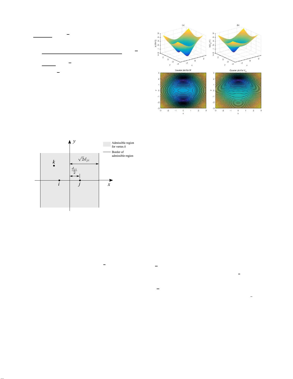
Directed F ormation Control of n Planar Agents with Distance and Area Constraints T airan Liu, Marcio de Queiroz, Pe ngpeng Zhang and Milad Kh aledyan Abstract — In this paper , we take a first step towards general- izing a recently proposed method f or d ealing with the problem of con ver gence to in correct equilibriu m points of d istance-based fo rmation controllers. Specifi cally , we in t roduce a distance and area-base d sch eme f or th e f ormation control of n -agent systems in two dimensions u sing directed graphs and the single- integrator model. W e show that under certain condit i ons on t h e edge lengths of the triangul ated desired form ation, th e control ensures almost-global conv ergence to the correct fo rmation. I . I N T RO D U C T I O N Formation contro l is an importan t pr oblem in mu lti-agent coordin ation an d cooperation where the objecti ve is f or agents to f orm a prescribed g eometric sha pe in spac e . This requirem ent is intr insic to tasks such as area coverage, perimeter protection , and co-tr a nsportation of large o bjects. One of two metho ds are typically used in formation control: i) regulate the r elative p osition of certain agent pair s to prescribed values [ 1], [2], or ii) re gulate a set of inter- agent distances (magnitu de of the relative p osition vector) to prescrib ed values [3], [4]. The first m ethod requires the agents to have a com mon global coor dinate frame or that their local coo rdinate frames b e aligned which may n ot be feasible in practice. On the other hand, the feedback variables in the secon d method can be c a lculated in each agen t’ s lo cal coordin ate f rame, wh ic h do not hav e to be aligned with a global coord inate fram e or with e a c h other . As a result, the desired fo rmation is, at best, on ly acq uired up to translation and rotation; i.e., the agen ts can conv erge to any formation that is isomorp hic to the desired on e. An imp ortant conside r ation in the d istance-based metho d is h ow to prevent agents from conver ging to a forma tio n that is equ ivalent but n oncong ruent to the d e sired one (see Section II-A for the form al defin itions o f equiv alency and congru ency). Such f o rmations are undesira b le be c ause they do not have th e same shape or orien tation as the pre scr ibed formation , althou gh the y satisfy th e set of distance con- straints. In o ther w ords, the distance constraints do not uniquely d efine th e relative positions o f th e age n ts and lead to positiona l amb ig uities [5]. Rigid graph theory pr ovid es a partial solutio n to this p roblem by requiring th e fo rmation graph to be rigid [6 ], [7]. Sp ecifically , imposing a m in imum number of distances to be controlled reduces the undesirab le T ai ran Liu, Marcio de Queiroz , and P engpeng Zhang are with the Departmen t of Mechanica l and Industrial Engineeri ng, Louisiana State Uni- versi ty , Baton Rouge, LA 70803, USA (Email: tliu7@lsu.edu; mdeque1@lsu.e du; pzhan16 @lsu.edu). Milad Khaledy an is with the Department of E lectri cal and Computer E ngineeri ng, Uni- versi ty of New Mexico , Alb uquerque, NM 87131, USA (Email: milad@unm.edu ). “equilibriu m p o ints” to fo rmations th a t are flipped/reflecte d versions of the desired one [ 5 ]. Th en, the determin ing factor whether convergence is to a congru ent fo rmation or a flipped formation is the initial conditio n of the r ig id formation. That is, rigidity distance-based f ormation con trollers on ly h av e local stab ility properties. A few appr oaches hav e been recently pr oposed to ad d ress the afo r emention e d issues with distance-b ased controller s. I n [8], a comb ination of in ter-agent distance an d angular con- straints was used to red uce the likelihood of convergence to nonco n gruen t fo rmations in two dimen sions (2D). Althoug h the region of attraction of th e de sired e q uilibrium can be somewhat enlarged b y a pro per choice of co ntrol g a ins, the stability of the control proposed in [8] is still loca l in n a ture. An extension of this work to 3D app eared in [ 9] by using ar e a and volume constraints. T he control method avoids flipped formation s but introduces o ther undesired equilibrium points due to the multiple local minim a of the pro posed potential function . A re lated appr oach was intr o duced in [10] fo r the single-integrator agent model where th e signed area o f a triangle was e m ployed as a controlled variable to prevent flipped form ations. That is, the sign o f the area enc losed by the for mation a long with th e inter-agent distances were used to u n iquely define the correct fo rmation up to translatio n and ro tation. The fo rmation contro l law in [10] was based on the gradient of a p otential func tio n that incorpora tes d istan ce error an d signed are a error term s and o n the u se of undir ected graphs (i.e., bid irectional sen sing and con trol). Co nvergence analyses were cond ucted f or special cases o f 3- and 4- a gent planar form ations. The pu rpose o f this paper is to explore the approa ch intro- duced in [10] f urther . Specifically , we aim to gener alize the approa c h to systems of n ag ents while intro ducing explicit, sufficient condition s for convergence to th e 2D desired for- mation. The key to o ur solutio n is triangu lating the dir e cted formation graph to facilitate the use o f in terconn e cted system theory . The u se of a directed g r aph has the ad ded benefit o f leading to a unidirection a l fo rmation con troller . Unde r our solution, mild conditions ar e imposed on th e ed ge len gths of the intercon nected trian gles, and the overall form ation graph is requ ired to b e a L eader-First-Follo wer (LFF) type o f minimally p ersistent directed gr aph [1 1]. W e show that our gradient- type co ntrol law ensures conv ergence to the d e sired formation a s lo ng as th e lead e r an d first follower are no t initially collocated. Th at is, no restrictions are p la c e d on the initial co n ditions of the ordinar y followers. The clo sed-loop system is proven to have an a lmost-globa l asymptotic equi- librium point correspon ding to the desired form ation. Th u s, the colline ar inv ariant set and flip ped form ation pro blems are hereby solved by the pro posed c o ntrol scheme. W e note that our result is no t a straigh tforward extension of [1 0] since th e interconn ected trian gles for m coupled n onlinear subsystems, which complicates the stability analysis of the overall system. I I . B AC K G RO U N D M AT E R I A L A. Undir ected Graph s An u ndirected graph G is represente d b y a pa ir ( V , E ) , where V = { 1 , 2 , ..., n } is the set of vertices and E = { ( i, j ) | i, j ∈ V , i 6 = j } ⊂ V × V is a set of und ir ected edges. The to tal numb er of edg es in E is denoted b y a ∈ { 1 , ..., n ( n − 1) / 2 } . Th e set o f neigh b ors of vertex i ∈ V is represented by N i ( E ) = { j ∈ V | ( i, j ) ∈ E } . (1) If p = [ p 1 , ..., p n ] ∈ R 2 n where p i ∈ R 2 is the coor dinate of the i th vertex, the n a fram ew ork F is d efined as the pair ( G, p ) . The edge functio n γ : R 2 n → R a is defined as γ ( p ) = [ ..., || p i − p j || 2 , ... ] , ( i, j ) ∈ E (2) such th at its m th compone n t, || p i − p j || , relates to the m th edge of E connecting the i th and j th vertices. The rigidity matrix R : R 2 n → R a × 2 n is given b y R ( p ) = 1 2 ∂ γ ( p ) ∂ p (3) where we hav e that ran k [ R ( p )] ≤ 2 n − 3 [6]. Fr amew ork s ( G, p ) a n d ( G, ˆ p ) are equ iv alent if γ ( p ) = γ ( ˆ p ) , and are congru ent if || p i − p j || = || ˆ p i − ˆ p j || , ∀ i , j ∈ V [12]. An isometry of R 2 is a map T : R 2 → R 2 satisfying [7] || w − z || = ||T ( w ) − T ( z ) || , ∀ w , z ∈ R 2 . (4) This map inclu des ro tation and translation of the vector w − z . T wo framew ork s are isomorp hic if they are corr elated via an isometry . It is obvio u s that (2 ) is inv ariant und er isomorph ic motions of the framework. A framework F = ( G, p ) is rigid in R 2 if all of its motions satisfy p i ( t ) = T ( p i ) , ∀ i ∈ V and ∀ t ∈ [0 , 1] ; i.e., the family o f fram eworks F ( t ) is isomorphic [6], [7]. Some related notions of rigidity ar e the following. A gener ic framework ( G, p ) is infinitesima lly rigid if and only if rank [ R ( p )] = 2 n − 3 [7 ]. A rig id f ramework is said to be minimally rigid if and on ly if a = 2 n − 3 [5]. I f the in finitesimally rig id f r amew ork s ( G, p ) and ( G, ˆ p ) a r e equiv alent but not con gruent, then th ey are refer red to a s ambiguo us [5] since th e edge fu nction canno t uniq uely defin e the framework. Common type s of am biguities are shown in Figure 1. Note that reflected f rameworks are an extreme fo rm of flip ambig uity w h ere m ore than one vertex is flipped. In fact, reflection s are the only fo rm of flip amb iguity that can occur in a triangular framework. B. Dir ected Graph s A directed gr aph G is a pair ( V , E d ) where th e ed ge set E d is directed in the sense that if ( i, j ) ∈ E d then i is the source vertex of the ed ge and j is the sink vertex. For i ∈ V , the out-d egree of i (d enoted by out ( i ) ) is the n u mber o f edges in E d whose sourc e is vertex i an d sinks are in V − { i } . Fig. 1. T ypes of ambiguous frame works. For directed grap hs, th e notion o f rigidity defin ed in Sec- tion II-A is no t e n ough to maintain th e f o rmation structure (see [13] for an examp le), and two additiona l co ncepts are needed. The first one is the no tion of a con straint consistent gr aph. As explained in [13], the intuitive meanin g of constraint consistency is that ev ery agent is able to satisfy all its distan ce constraints when all the others are trying to do the same. A sufficient conditio n fo r a directed g raph  V , E d  in R 2 to be constraint consistent is that ou t ( i ) ≤ 2 for all i ∈ V (see Lem ma 5 of [14]). The secon d co ncept is gra p h persistency , which has the meaning tha t, provided all agents are tryin g to satisfy their distance co nstraints, the structure of the agent fo rmation is preserved [ 13]. A directed graph is persistent if and only if it is co n straint consistent and its un derlying und irected gr aph is infinitesimally rigid (see Theor em 3 o f [14]). A persistent grap h in R 2 is said to be minimally persistent if no sin g le edge can b e removed without lo sing per sistence. A n e cessary con dition for a persistent graph in R 2 to be min im ally persistent is out ( i ) ≤ 2 for all i ∈ V , while a sufficient co ndition is minimal rigidity [ 14]. Starting fr om two vertices with an edge, a minimally persistent (resp., rig id) g raph can be constru cted by the Henneberg insertion of type I [15], i.e., iteratively adding a vertex with two o utgoing (resp. , und irected) edges. Hencefor th , we refer to a g raph constructed in this manne r as a Henneb e rg gra p h. C. Signed Ar ea The signed ar ea of a trian gular framework, S : R 6 → R , is d efined as [10] S ( p ) = 1 2 det  1 1 1 p 1 p 2 p 3  = 1 2 ( p 3 − p 1 ) ⊺ J ( p 3 − p 2 ) (5) where J =  0 1 − 1 0  . (6) This quantity is positive ( resp., negati ve) if the vertices a r e ordered c o unterclo ckwise (resp., clockwise) . Further, (5) is zero if any two vertices are collocated o r the th r ee vertices are co llinear . A Henn eberg fra m ew ork can be divided into triangular sub-fram ew orks. Ther e fore, th e signed are a of a Henneberg framework with n vertices an d direc ted edge set E d , χ : R 2 n → R n − 2 , is defined as χ ( p ) =  ..., 1 2 det  1 1 1 p i p j p k  , ...  , ∀ ( k , i ) , ( k, j ) ∈ E d − { (2 , 1) } (7) such that its m th compo nent is related to the signed are a of the m th triangle co nstructed with vertices i , j , an d k . For example, the signed area of the framework in Figu re 2a is giv en b y χ ( p ) = h 1 2 ( p 3 − p 1 ) ⊺ J ( p 3 − p 2 ) , 1 2 ( p 4 − p 2 ) ⊺ J ( p 4 − p 3 ) , 1 2 ( p 5 − p 3 ) ⊺ J ( p 5 − p 4 ) i , (8) where the thre e elements of χ ( p ) are po siti ve, negativ e, an d positive, respectively . For the f ramework in Figu re 2b, it would b e χ ( p ) = h 1 2 ( p 3 − p 1 ) ⊺ J ( p 3 − p 2 ) , 1 2 ( p 4 − p 1 ) ⊺ J ( p 4 − p 2 ) , 1 2 ( p 5 − p 3 ) ⊺ J ( p 5 − p 4 ) i . (9) Fig. 2. Signed area examples. W e introduce ne xt is an extension of th e concept of congru ency that in c lu des the signe d ar ea. Definition 1: Henneb erg frameworks F = ( G, p ) and ˆ F = ( G, ˆ p ) where G = ( V , E ) ar e said to be str ongly congruen t if th ey are cong ruent and χ ( p ) = χ ( ˆ p ) . W e repr esent the set o f all frameworks that are stron gly congru ent to F by SCgt ( F ) . It is o bvious th at frameworks that ar e co ngruen t but not strongly con gruen t are r eflected frameworks. Note that if ˆ F is a reflected version of F , then χ ( p ) = − χ ( ˆ p ) . In sum mary , the signed area f u nction will be used to rule o u t the the o ccurren ce o f framework amb ig uities, especially reflections. Lemma 1 : Henneberg fra m ew orks F = ( G, p ) and ˆ F = ( G, ˆ p ) are strongly con gruent if and on ly if th ey ar e equ iv- alent an d χ ( p ) = χ ( ˆ p ) . Pr oof: See Append ix VI-A. D. Quartic P olyno mials Lemma 2 : [16], [17], [18], [ 19] For any q uartic polyn o - mial equatio n ax 4 + b x 3 + cx 2 + dx + e = 0 wher e a 6 = 0 , Λ = 256 a 3 e 3 − 1 92 a 2 bde 2 − 1 28 a 2 c 2 e 2 + 1 44 a 2 cd 2 e − 2 7 a 2 d 4 + 1 44 ab 2 ce 2 − 6 ab 2 d 2 e − 80 abc 2 de + 1 8 abcd 3 + 1 6 ac 4 e − 4 ac 3 d 2 − 2 7 b 4 e 2 + 1 8 b 3 cde − 4 b 3 d 3 − 4 b 2 c 3 e + b 2 c 2 d 2 , P =8 a c − 3 b 2 , D =64 a 3 e − 16 a 2 c 2 + 1 6 ab 2 c − 1 6 a 2 bd − 3 b 4 , the equa tion has n o real solution if Λ > 0 and P > 0 , o r Λ > 0 and D > 0 . Cor ollary 1 : Consider the equation ax 4 + b x 3 + cx 2 + dx + e = 0 (10) where a = − 2 δ 2 1 ( γ − 2) 2 b = δ 1 ( γ 2 − 4 ) q 2 δ 2 1 δ 2 2 − δ 4 1 + 2 δ 2 1 δ 2 3 − δ 4 2 + 2 δ 2 2 δ 2 3 − δ 4 3 c = − 1 2 δ 4 1 γ 3 + δ 2 1  3 2 δ 2 1 + δ 2 2 + δ 2 3  γ 2 − 4 δ 2 1  δ 2 2 + δ 2 3  γ d = 1 4 δ 1 γ 2 (2 δ 2 1 γ − 3 δ 2 1 − 2 δ 2 2 − 2 δ 2 3 ) × q 2 δ 2 1 δ 2 2 − δ 4 1 + 2 δ 2 1 δ 2 3 − δ 4 2 + 2 δ 2 2 δ 2 3 − δ 4 3 e = − 1 8 δ 2 1 γ 3 (2 δ 2 1 δ 2 2 − δ 4 1 + 2 δ 2 1 δ 2 3 − δ 4 2 + 2 δ 2 2 δ 2 3 − δ 4 3 ) , γ is a positive constant, and δ 1 , δ 2 , δ 3 are th e leng ths of the edges of a triangle. If δ 2 6 = δ 3 and     δ 2 3 − δ 2 2 δ 2 1     < 2 √ 2 , (11) then ther e exists a γ > 0 suc h that (10) has n o real solu tion for γ > max { γ , 2 } . Pr oof: See Append ix VI-B. Remark 1 : The geometr ic mea n ing o f co ndition (11) is discussed in Remark 3 . Althou g h the existence of the lower bound γ in Co r ollary 1 is g uaranteed , a clo sed -form expr e s- sion for γ does not exist in g eneral. Howev er, γ can be easily determ in ed by num e rical mean s onc e δ 1 , δ 2 , and δ 3 are selected . E. Stability Results Lemma 3 : [20] Consider th e system ˙ x = f ( x, u ) where x is the state, u is the control input, an d f ( x, u ) is locally Lipschitz in ( x, u ) in some neighb orhoo d of ( x = 0 , u = 0) . Then, the system is locally input-to-state stable if and only if the unfor ced system ˙ x = f ( x, 0 ) h as a locally asympto tically stable equilibr ium point at the or igin. Lemma 4 : [21] Consider the interco nnected system Σ 1 : ˙ x = f ( x, y ) Σ 2 : ˙ y = g ( y ) . (12) If su b system Σ 1 with inp ut y is locally input- to-state stable and y = 0 is a locally asymp totically stable equilibrium po int of subsystem Σ 2 , then [ x, y ] = 0 is a locally asymp totically stable equilibr ium point of the interc o nnected system. I I I . P R O B L E M S T A T E M E N T Consider a system of N ≥ 2 mobile agen ts governed by the kinem a tic equation ˙ p i = u i , i = 1 , ..., N (13) where p i ∈ R 2 is the position of the i th agent relative to an Earth-fixed coo r dinate f r ame, and u i ∈ R 2 is the velocity- lev el c o ntrol in p ut. The desired formation o f agents is mod eled b y the di- rected framework F ∗ = ( G ∗ , p ∗ ) where G ∗ = ( V ∗ , E ∗ ) , dim( E ∗ ) = a , p ∗ = [ p ∗ 1 , ..., p ∗ N ] , and p ∗ i ∈ R 2 denotes the desired position of the i th ag ent. T he fixed desired distanc e separating th e i th and j th agents is defined as d j i = || p ∗ j − p ∗ i || > 0 , i, j ∈ V ∗ (14) W e assume F ∗ is con structed to satisfy the following co n - ditions: Condition 1 out (1) = 0 , out (2) = 1 , and ou t ( i ) = 2 , ∀ i ≥ 3 . Condition 2 If ther e is an edge between agen ts i a nd j , the direction must be i ← j if i < j . The above con ditions imply that F ∗ should be a LFF- type minimally persistent form ation [1 1], wh e re agen t 1 is the leader, agent 2 is the first f ollower , an d agen ts i fo r i ≥ 3 are ca lled ordinar y followers. The actual fo rmation o f ag ents is mod e led by F ( t ) = ( G ∗ , p ( t )) wher e p = [ p 1 , ..., p N ] . Note that F and F ∗ share the sam e dir ected graph, which remains u nchang ed for all time. The physical meaning o f ( j, i ) ∈ E ∗ in the actual formation is th at ag ent j ca n m easure its relative position to agent i , p j − p i , but not vice versa. The control objective of th is p aper is to en su re F ( t ) → SCgt ( F ∗ ) a s t → ∞ , (15) which is equiv alent to saying || p j ( t ) − p i ( t ) || → d j i as t → ∞ , i, j ∈ V ∗ and (16a) χ ( p ( t )) → χ ( p ∗ ) a s t → ∞ . (16b) The control objective will be q uantified by two types of error variables. If the relative position o f two agents is defined as ˜ p j i = p j − p i , the distan c e err or is g iven by [4] z j i = || ˜ p j i || 2 − d 2 j i . (17) The stacked vector of all distances errors is defined as z = [ z 21 , ..., z j i , ... ] , ∀ ( j, i ) ∈ E ∗ . The a r ea err or is de fined as [10] ˜ S ij k = S ij k − S ∗ ij k , ( k , i ) , ( k , j ) ∈ E ∗ (18) where S ij k = S ( p ) with p = [ p i , p j , p k ] and S ∗ ij k = S ( p ∗ ) with p ∗ = [ p ∗ i , p ∗ j , p ∗ k ] . The stacked vecto r of all a r ea error s is g iv en by ˜ S = [ ˜ S 123 , ..., ˜ S ij k , ... ] , ∀ ( k , i ) , ( k , j ) ∈ E ∗ . Since F ∗ is ty pically specified in terms of the d esired inter-agent d istances, a useful f ormula for calculating S ∗ ij k is g iv en by [22] S ∗ ij k = ± q d ij k ( d ij k − d j i ) ( d ij k − d ki ) ( d ij k − d kj ) (19) where d ij k = d j i + d ki + d kj 2 . (20) Note that if the o r der of ag ents i, j, k is counterclo ckwise (resp., clockwise), th en (19) takes the positive (resp., n ega- ti ve) sign. I V . C O N T R O L L AW F O R M U L AT I O N The control law will be dictated by the choice of potential function associa te d with the error variables (1 7) an d (18). T o this end, we con sider the L yapunov function candid ate [10] V k =    α 2 4 z 2 21 , if k = 2 α k 4  z 2 ki + z 2 kj  + β k ˜ S 2 ij k , if 2 < k ≤ N (21) where α k and β k are p ositiv e constants, i < j < k , an d ( k , i ) , ( k , j ) ∈ E ∗ . Based on (21) and its time der i vati ve, we prop ose the following contro l law u 1 = 0 (22a) u 2 = − α 2 z 21 ˜ p 21 (22b) u k = − α k ( z ki ˜ p ki + z kj ˜ p kj ) − β k ˜ S ij k J ⊺ ( ˜ p ki − ˜ p kj ) (22c) for 2 < k ≤ N , i < j < k , an d ( k , i ) , ( k , j ) ∈ E ∗ . The control law is only a functio n of ˜ p ki , ˜ p kj , d ki , d kj and d j i for i, j ∈ N k ( E ∗ ) . Thu s, the co ntrol law is d istributed since it on ly requires the k th agent to m e asure its rela tive position to neigh b oring agents in the directed gr a ph. The following theorem states ou r main re su lt. Theor em 1: Let the initial co nditions o f th e f ormation F ( t ) = ( G ∗ , p ( t )) be such that p 1 (0) 6 = p 2 (0) , an d let F ∗ satisfy      d 2 ki − d 2 kj d 2 j i      < 2 √ 2 , (23) for all i, j, k such that 2 < k ≤ N , i < j < k , an d ( k , i ) , ( k, j ) ∈ E ∗ . Then, the contr ol (22) with β k α k >    d 2 kj − d 2 j i / 4 d 2 j i , if d ki = d kj γ , if d ki 6 = d kj (24) where γ is deter mined fro m Corollary 1, ren ders h z , ˜ S i = 0 asymptotically stable and ensures F ( t ) → SCgt ( F ∗ ) as t → ∞ . Pr oof: The op en-loop dynamics for ( 1 7) and ( 18) are g iv en by ˙ z j i = 2 ˜ p ⊺ j i ( u j − u i ) (25) and · ˜ S ij k = 1 2 [( u k − u i ) ⊺ J ˜ p kj + ˜ p ⊺ ki J ( u k − u j )] , (26) where (1 3) was u sed. Ther efore, th e time derivati ve of (2 1) becomes ˙ V k =                α 2 z 21 ˜ p ⊺ 21 ( u 2 − u 1 ) , if k = 2 α k  z ki ˜ p ⊺ ki ( u k − u i ) + z kj ˜ p ⊺ kj ( u k − u j )  + β k ˜ S ij k  ( u k − u i ) ⊺ J ˜ p kj + ˜ p ⊺ ki J ( u k − u j )  , if 2 < k ≤ N (27) Step 1: Consider the subsystem composed of agents 1 an d 2 only . Substituting (22a) and (22b ) into (25 ) yield s ˙ z 21 = − 2 α 2 z 21 || ˜ p 21 || 2 = − 2 α 2 z 21  z 21 + d 2 21  (28) where (17) was used. The solution to the ab ove no nlinear ODE is z 21 ( t ) = d 2 21 z 21 (0) d 2 21 exp(2 d 2 21 α 2 t ) ( z 21 (0) + d 2 21 ) − z 21 (0) . (29) From (17) , it is clear that z 21 ∈  − d 2 21 , ∞  where z 21 = − d 2 21 correspo n ds to agents 1 and 2 being collocated . If z 21 (0) > − d 2 21 , we can sh ow from (2 9 ) th at z 21 ( t ) > − d 2 21 ∀ t > 0 as fo llows: z 21 ( t ) > − d 2 21 ⇔ z 21 (0) d 2 21 exp(2 d 2 21 α 2 t ) ( z 21 (0) + d 2 21 ) − z 21 (0) > − 1 ⇔ z 21 (0) > z 21 (0) − d 2 21 exp(2 d 2 21 α 2 t )  z 21 (0) + d 2 21  ⇔ d 2 21 exp(2 d 2 21 α 2 t )  z 21 (0) + d 2 21  > 0 ⇔ z 21 (0) > − d 2 21 . (30) Now , af ter substituting (22 a) and ( 2 2b) in to (27), we obtain ˙ V 2 = − α 2 2 z 2 21 || ˜ p 21 || 2 ≤ 0 . (31) Since z 21 ( t ) > − d 2 21 implies || ˜ p 21 ( t ) || > 0 , we can see tha t ˙ V 2 = 0 on ly at z 21 = 0 . Th e r efore, ˙ V 2 is negative definite and z 21 = 0 is asy mptotically stable for z 21 (0) > − d 2 21 (or equiv alently , p 1 (0) 6 = p 2 (0) ). Step 2: Consider th at a thir d agent is added to the p revious subsystem as shown in Figure 3. W e can view this n ew system as the intercon nected system ˙ ξ 3 = f 3 ( ξ 3 , Ξ 2 ) (32a) ˙ Ξ 2 = g 3 (Ξ 2 ) (32b) where ξ 3 := [ z 31 , z 32 , ˜ S 123 ] is th e state of the error dynam ics of agent 3 and Ξ 2 = ξ 2 := z 21 . Fig. 3. Three-agent system. W e seek to estab lish the inp ut-to-state stab ility of (32 a) with r espect to in put Ξ 2 via Lemma 3 . Whe n Ξ 2 = 0 , we can see from ( 22b) that u 2 = 0 . Therefor e, fr om (27) with k = 3 under the con d ition that Ξ 2 = 0 , we have that ˙ V 3 = h α 3 ( z 31 ˜ p 31 + z 32 ˜ p 32 ) ⊺ + β 3 ˜ S 123 ( ˜ p 31 − ˜ p 32 ) ⊺ J i u 3 . (33) Substituting ( 22c) with k = 3 in (33 ) gives ˙ V 3 = −    α 3 ( z 31 ˜ p 31 + z 32 ˜ p 32 ) + β 3 ˜ S 123 J ⊺ ( ˜ p 31 − ˜ p 32 )    2 . (34) If ξ 3 = 0 is the only value at which ˙ V 3 = 0 , th en (33 ) is negati ve d efinite and (32a) is input-to-state stable. I t then fo llows that the o rigin of (3 2), i.e., [Ξ 2 , ξ 3 ] = 0 , is asymptotically stable accordin g to Lemma 4. T o this en d, note that translation al and rotation al motion s of the triangle will n ot chan g e the value of ˙ V 3 since it is a function of the relativ e po sition of agen ts and th e triangle area [23], [2 4]. Thus, witho ut th e loss of generality , let p 1 = [ − d 21 / 2 , 0] , p 2 = [ d 21 / 2 , 0] , an d p 3 = [ x, y ] fo r simplicity . T hen, ˙ V 3 = 0 is eq uiv alent to  2 x 2 + 2 y 2 + d 2 21 2 − d 2 32 − d 2 31  x + d 21 2  2 d 21 x − d 2 31 + d 2 32  = 0 and  2 x 2 + 2 y 2 + d 2 21 2 − d 2 32 − d 2 31  y + β 3 α 3  d 2 21 2 y − d 21 S ∗ 123  = 0 . (35) One so lu tion to (35) is x =  d 2 31 − d 2 32  / (2 d 21 ) and y = 2 S ∗ 123 /d 21 , (36) which co rrespond s to ξ 3 = 0 . W e will show next that β 3 /α 3 can be selected such that this is the only solution to ( 35). This proof will be conduc te d fo r two distinct cases: an isosceles triangle and the non- isosceles case. (Case 2a) Con sider that the trian gle is such that d 32 = d 31 . From (35), we get  2 x 2 + 2 y 2 + 3 d 2 21 2 − 2 d 2 32  x = 0 and  2 x 2 + 2 y 2 + 1 2 d 2 21 − 2 d 2 32  y + β 3 2 α 3 d 2 21  y − 1 2 q 4 d 2 32 − d 2 21  = 0 . (37) The first eq uation o f (3 7) implies x = 0 or x 2 + y 2 = d 2 32 − 3 4 d 2 21 . Sub stituting x = 0 into th e second eq uation o f (37) y ields  y − 1 2 q 4 d 2 32 − d 2 21  ×  8 y 2 + 4 q 4 d 2 32 − d 2 21 y + 2 β 3 α 3 d 2 21  = 0 . (38) It is easy to show that when β 3 α 3 > d 2 32 − 1 4 d 2 21 d 2 21 , (39) the discrimin ant of 8 y 2 + 4 p 4 d 2 32 − d 2 21 y + 2 β 3 α 3 d 2 21 is less than 0. Th at is, ine q uality (3 9) will lead to x = 0 and y = 1 2 p 4 d 2 32 − d 2 21 being the only solution to (38 ). Now , su b stituting x 2 + y 2 = d 2 32 − 3 4 d 2 21 (40) into th e second equation of (3 7) gives 2 y  β 3 α 3 − 2  = β 3 α 3 q 4 d 2 32 − d 2 21 . (41) After squaring ( 41) an d using (4 0) ag ain to eliminate y , we obtain 2 x 2  β 3 α 3 − 2  2 = − " d 2 21  β 3 α 3  2 +  8 d 2 32 − 6 d 2 21  β 3 α 3 + 6 d 2 21 − 8 d 2 32 # | {z } . φ ( β 3 /α 3 ) (42) Since th e lef t han d side of (4 2) is no nnegative for any β 3 /α 3 , this equatio n has no solution if φ ( β 3 /α 3 ) > 0 . Th is means that φ ( β 3 /α 3 ) should have n o real roots, o r β 3 /α 3 should be chosen to be gr eater (resp. , smaller) than the largest (resp., smallest) roo t. Th e discriminant of φ ( β 3 /α 3 ) is given by ∆ = 4  4 d 2 32 − 3 d 2 21   4 d 2 32 − d 2 21  . (43) If 4 3 d 2 32 < d 2 21 < 4 d 2 32 , then ∆ < 0 for any β 3 /α 3 > 0 and φ ( β 3 /α 3 ) > 0 . If d 2 21 ≤ 4 3 d 2 32 , then ∆ ≥ 0 an d φ ( β 3 /α 3 ) h as real roots. Since the smallest root is less than ze ro, the only o ption for ensuring φ ( β 3 /α 3 ) > 0 is to ch oose β 3 /α 3 greater th an th e largest roo t, i.e., β 3 α 3 > 3 d 2 21 − 4 d 2 32 + p (4 d 2 32 − 3 d 2 21 )(4 d 2 32 − d 2 21 ) d 2 21 . (44) Note that th e case where d 2 21 ≥ 4 d 2 32 is not possible since it contradicts the fact that d 32 + d 31 = 2 d 32 > d 21 . Combining the three cases, we see that (41 ) will have no solution if ( 44) ho lds. Fina lly , it is no t difficult to show that (39) is a sufficient condition f or (4 4). There f ore, for the isosceles triang le, the condition fo r ξ 3 = 0 to b e the on ly value where ˙ V 3 = 0 is g iven by (39) . (Case 2b) Consider that the triangle is not isosceles ( d 32 6 = d 31 ) . Afte r substituting th e first eq uation of (35) in to the seco nd one, eliminating x , and factoring the resulting polyno mial of y , we ob tain  y − 2 S ∗ 123 d 21   c 4 y 4 + c 3 y 3 + c 2 y 2 + c 1 y + c 0  = 0 (45 ) where c 4 = − 2 d 2 21  β 3 α 3 − 2  2 (46a) c 3 = d 21 "  β 3 α 3  2 − 4 # × q 2 d 2 21 d 2 32 − d 4 21 + 2 d 2 21 d 2 31 − d 4 32 + 2 d 2 32 d 2 31 − d 4 31 (46b) c 2 = − 1 2 d 4 21  β 3 α 3  3 + d 2 21  3 2 d 2 21 + d 2 32 + d 2 31   β 3 α 3  2 − 4 d 2 21  d 2 32 + d 2 31  β 3 α 3 (46c) c 1 = 1 4 d 21  β 3 α 3  2  2 d 2 21 β 3 α 3 − 3 d 2 21 − 2 d 2 32 − 2 d 2 31  × q 2 d 2 21 d 2 32 − d 4 21 + 2 d 2 21 d 2 31 − d 4 32 + 2 d 2 32 d 2 31 − d 4 31 (46d) c 0 = − 1 8 d 2 21  β 3 α 3  3 ×  2 d 2 21 d 2 32 − d 4 21 + 2 d 2 21 d 2 31 − d 4 32 + 2 d 2 32 d 2 31 − d 4 31  . (46e) Note that the qu artic polynomia l in (45) is similar to (10). Thus, by Corollary 1, if     d 2 31 − d 2 32 d 2 21     < 2 √ 2 (47) and β 3 /α 3 > max { γ , 2 } (see pr oof of Corollary 1 for detail of γ ), th e qu a rtic polyn omial has no real solu tion, and y = 2 S ∗ 123 /d 21 is th e only solution to (45 ). Step k: The pro cess o f add ing a vertex k with two outgoin g edges to any two distinct vertices i an d j of the previous graph can be fo llowed on e step at a time, resulting at each step in th e intercon nected system ˙ ξ k = f k ( ξ k , Ξ k − 1 ) (48a) ˙ Ξ k − 1 = g k (Ξ k − 1 ) (48b) where ξ k := [ z ki , z kj , ˜ S ij k ] , ( k , i ) , ( k, j ) ∈ E ∗ is the state o f error d ynamics of the k th age nt an d Ξ k − 1 := [ ξ 2 , ..., ξ k − 1 ] . Note that the asy mptotic stability of Ξ k − 1 = 0 for (48b) was already established in Step k − 1 . Ther efore, we o nly need to chec k the inp ut-to-state stability of (48a) with respect to input Ξ k − 1 . T o this en d, when Ξ k − 1 = 0 , (27 ) becom es ˙ V k = h α k ( z ki ˜ p ki + z kj ˜ p kj ) ⊺ + β k ˜ S ij k ( ˜ p ki − ˜ p kj ) ⊺ J i u k . (49) Now , su b stituting (2 2 c) in to ( 4 9) gives ˙ V k = −    α k ( z ki ˜ p ki + z kj ˜ p kj ) + β k ˜ S ij k J ⊺ ( ˜ p ki − ˜ p kj )    2 . (50) Similar to Step 2, we can show that if the gain ratio β k /α k is selected accord ing to (2 4) and the edg es of triangle ∆ ij k satisfy (23 ), then (50 ) is negative definite. As a r esult, (48a) is input-to-state stable and [Ξ k − 1 , ξ k ] = 0 in (48) is asymptotically stable by Lemm a 4. Repeating this p rocess until k = N lead s to th e conclu sion that [ ξ 2 , ..., ξ N ] = 0 is asymptotically stable, wh ic h im plies z ( t ) → 0 and χ ( p ( t )) → χ ( p ∗ ) a s t → ∞ . G iven that F ∗ and F ( t ) have the same edg e set and F ∗ is minimally persistent by de sig n, then we h av e that F ( t ) → SCgt ( F ∗ ) as t → ∞ from Lemm a 1. Remark 2 : Theorem 1 only requires tha t the lead e r an d first fo llower not be collo cated at t = 0 . If agents 1 and 2 were in itialized at th e same position, then u 1 = u 2 = 0 and they would re m ain at this position for ev er . I n other words, the condition p 1 = p 2 is an inv ariant set. As for the ord inary followers, ( 22) guar antees f ormation acquisition r egar dless of their initial co nditions. For examp le, if agents 2, 3, 4 , and 5 in Figu re 2 ar e all in itially collo cated, then u 4 = u 5 = 0 at t = 0 which means ag ents 4 and 5 will not move at first. Howe ver , u 3 6 = 0 , so ag ent 3 will move. Th is results in u 4 6 = 0 , cau sing agen t 4 to move, and finally u 5 becomes nonzer o , so agent 5 moves. Remark 3 : Condition (2 3) on th e desired for mation has the following geo metric inter pretation. Consider the three vertices in Figu re 4 where, for simplicity , p ∗ i = [ − d j i / 2 , 0] , p ∗ j = [ d j i / 2 , 0] , and p ∗ k = [ x, y ] . 1 1 Tra nslation and rotati on of these vertice s as a rigi d body will not affec t the followi ng analysis since it is only depe ndent on their dista nces. Giv en that      d 2 ki − d 2 kj d 2 j i      < 2 √ 2 ⇐ ⇒    ( x + d j i / 2) 2 + y 2 − ( x − d j i / 2) 2 − y 2    d 2 j i < 2 √ 2 ⇐ ⇒ | 2 xd j i | d 2 j i < 2 √ 2 ⇐ ⇒ | x | < √ 2 d j i , (51) any p o int p ∗ k inside the shaded r egio n in Figu re 4 satisfies (23). It is importan t to point out that (23) is sufficient but not necessary fo r stability . For example, consid e r a tr iangular formation with d 21 = 1 , d 31 = 2 . 1 , and d 32 = 3 , which does not satisfy (23 ). If howe ver β 3 /α 3 is selected in the rang e (10 . 42 , 13 . 55) , the stability result of Theorem 1 will hold. In fact, the g ain ratio β k /α k and ( 2 4) impose a lower bound on the relative weight of the distance error and area error in the poten tial function (21) in ord er to gu arantee stability . Fig. 4. Geometeri c interpretati on of (23). Remark 4 : Mathematically , the role of the a rea-based term β k ˜ S 2 ij k is to guar antee the existence of a un ique minimum for th e po tential f unction (21) in th e Euclidean plane, and thus av oid th e system from co n verging to an u nde- sirable local minima. T o illustrate this, consider a triangu lar formation where p 1 = [ − 1 , 0] , p 2 = [1 , 0] , p 3 = [ x, y ] , an d d 21 = d 31 = d 32 = 2 , and let W = 1 4 ( z 2 31 + z 2 32 ) be the potential func tio n with only the distance e rror terms of (2 1) with k = 3 . In Figure 5, we plo t ln( W + 1 ) and ln( V 3 + 1) versus p 3 to have a better view o f th eir m in ima. 2 W e can clearly see th at W ( p 3 ) has two minima, co rrespon d ing to the desired position fo r agent 3 and its reflec ted position , whereas V 3 ( p 3 ) h as a uniqu e minimu m. V . C O N C L U S I O N S This pap e r presented a 2D formatio n control scheme that u ses distance and signed ar ea inf o rmation to guaran tee conv ergence to the desired for mation shape . Th e asymptotic conv ergence r esult is valid und er mild con ditions on th e 2 Since functio ns ln( V + 1) and V are positi vely correlate d, this varia ble change does not af fect the funct ion extre ma. Fig. 5. a) Potential function W ( q 3 ) and corresponding counter plot; b) Potenti al function V 3 ( q 3 ) and corresponding counte r plot. edge length s of the triangulated -like fr amew ork and when the leader agen t and the first fo llower are not colloca te d at time zer o. The scheme is ap plicable to sy stems with any number of agents governed by the single-in tegrator model. V I . A P P E N D I X A. Pr oof of Lemma 1 (Pr oof of ⇒ ) If F and ˆ F are stron gly congr uent, then || p i − p j || = || ˆ p i − ˆ p j || , ∀ i, j ∈ V and χ ( p ) = χ ( ˆ p ) by definition. Therefo r e, since E ⊂ V × V , we know || p i − p j || = || ˆ p i − ˆ p j || , ∀ ( i, j ) ∈ E , i.e., F and ˆ F ar e equivalent. (Pr oof of ⇐ ) If dim( V ) = 3 , then framework equ iv alency and con gruency a r e equ iv alent, so the cond itions f o r strong congru ency are tr ivially satisfied. If a vertex is added suc h that dim ( V ) = 4 , the result- ing framew ork would have two additio n al edges and one additional triangle. Consider without lo ss of generality the framework in Figure 6(a), wh ere the area o f th e quad rilateral is g iv en by S Q := S 123 − S 234 . Since χ ( p ) = χ ( ˆ p ) , we know that S Q ( p ) = S Q ( ˆ p ) , so it fo llows from th e gener al quadrilater al area formu la [22] that 1 4 h 4 k p 3 − p 2 k 2 k p 4 − p 1 k 2 −  k p 2 − p 1 k 2 + k p 4 − p 3 k 2 − k p 3 − p 1 k 2 − k p 4 − p 2 k 2  2 i 1 2 = 1 4 h 4 k ˆ p 3 − ˆ p 2 k 2 k ˆ p 4 − ˆ p 1 k 2 −  k ˆ p 2 − ˆ p 1 k 2 + k ˆ p 4 − ˆ p 3 k 2 − k ˆ p 3 − ˆ p 1 k 2 − k ˆ p 4 − ˆ p 2 k 2  2 i 1 2 . (52) Since F and ˆ F are equivalent, k p 2 − p 1 k = k ˆ p 2 − p 1 k , k p 3 − p 1 k = k ˆ p 3 − ˆ p 1 k , k p 3 − p 2 k = k ˆ p 3 − ˆ p 2 k , k p 4 − p 2 k = k ˆ p 4 − ˆ p 2 k , and k p 4 − p 3 k = k ˆ p 4 − ˆ p 3 k . Therefo re, we have fro m (5 2) th at k p 4 − p 1 k = k ˆ p 4 − ˆ p 1 k , so F and ˆ F are strongly congru e nt fo r dim ( V ) = 4 . Sinc e the quad rilateral signed area form ula in (52) ap plies to both conv ex and concave quadr ilaterals, a similar analy sis exists for all other cases, some of which are shown in Fig ure 6. Fig. 6. Con vex and concav e quadrila terals with five edges. As mo r e vertices ar e added, each ad d itional vertex will create a quad rilateral, so above pr ocess ca n be repeated to show that F and ˆ F are strong ly con gruent fo r dim( V ) = n . B. Pr oof of Cor ollary 1 Based o n Lem ma 2, ( 10) has n o real solution if the following quantities are positive: Λ = γ 6 ( γ − 2) 2 h − 1 16 δ 12 1  δ 2 2 − δ 2 3  2  8 δ 4 1 −  δ 2 2 − δ 2 3  2  ×  δ 4 1 − 2 δ 2 1  δ 2 2 + δ 2 3  +  δ 2 2 − δ 2 3  2  γ 7 + f 1 ( δ 1 , δ 2 , δ 3 , γ ) i (53a) P = ( γ − 2) 2  8 δ 6 1 γ 3 + f 2 ( δ 1 , δ 2 , δ 3 , γ )  (53b) where f 1 ( · ) and f 2 ( · ) are poly nomials in γ of, at most, degree 6 and 2, respectively . Giv en a p olynom ial p ( γ ) = a n γ n + P n − 1 i =0 a i γ i where n ≥ 3 is an odd integer, we c a n see from Figur e 7 that p ( γ ) = 0 has at least o ne real ro ot. Denote the largest or th e unique real roo t by γ ∗ . Then, p ( γ ) > 0 ∀ γ > γ ∗ , if a n > 0 p ( γ ) < 0 ∀ γ > γ ∗ , if a n < 0 . (54) Fig. 7. Odd de gree polynomia l. Consider th at γ 6 = 2 in (53a) and (53b) . It follows fro m the cond itions δ 2 6 = δ 3 and    δ 2 3 − δ 2 2  /δ 2 1   < 2 √ 2 that δ 4 1 − 2 δ 2 1 ( δ 2 2 + δ 2 3 ) + ( δ 2 2 − δ 2 3 ) 2 = ( δ 1 + δ 2 + δ 3 )( δ 1 − δ 2 − δ 3 )( δ 1 + δ 2 − δ 3 )( δ 1 − δ 2 + δ 3 ) < 0 . Therefo re, the coefficient of γ 7 in (53 a ) is p ositiv e, and Λ > 0 for γ > γ ∗ 1 where γ ∗ 1 is the lower b ound from (54). Like wise, the co e fficient of γ 3 in (53 b) is positive, and P > 0 for γ > γ ∗ 2 where γ ∗ 2 is some lower bound . Thu s, the overall sufficient cond ition for Λ > 0 and P > 0 is given by γ > max { γ , 2 } wher e γ := max { γ ∗ 1 , γ ∗ 2 } . R E F E R E N C E S [1] R. Olfati -Saber and R. M. Murray , “Consensus problems in netw orks of agents with switching topology and time-delays, ” IEEE T ransac- tions on Automatic Contr ol , vol. 49, no. 9, pp. 1520–153 3, 2004. [2] W . Ren and R. W . Beard, Distribut ed consensus in multi-vehi cle cooper ative contr ol . Springer -V erlag London, 2008. [3] F . Dorfler and B. Francis, “Geometric analysis of the formation problem for autonomous robots, ” IEEE T ransactio ns on Automatic Contr ol , vol . 55, no. 10, pp. 2379–2384, 2010. [4] L. Krick, M. E. Brouck e, and B. A. Francis, “Stabil isation of infinitesi- mally rigid formations of multi-robot networks, ” Internati onal Journal of Contro l , vol. 82, no. 3, pp. 423–439, 2009. [5] B. D. O. Anderson, C. Y u, B. Fidan, and J. M. Hendric kx, “Rigid graph control architectur es for autonomous formations, ” IEEE Contr ol Systems , vol. 28, no. 6, 2008. [6] L. Asimow and B. Roth, “The rigidity of graphs, II, ” J ournal of Mathemat ical Analysis and Applicati ons , vol. 68, no. 1, pp. 171–190, 1979. [7] I. Izmestie v , “Infinitesimal rigidity of framewo rks and surfaces, ” Lectur es on Infinitesimal Rigidity , K yushu Unive rsity , Japan , 2009. [8] E. D. Ferreira-V azquez , E. G. Hernandez -Martinez , J. J. Flores- Godoy , G. Fernandez-Anay a, and P . Paniagua-C ontro, “Distance- based formation control using angular information between robots, ” J ournal of Intellig ent & Robotic Systems , vol. 83, no. 3-4, pp. 543–560, 2016. [9] E. D. Ferreira-V azquez, J. J. Flores-Godo y , E . G. Hernandez-Mart inez, and G. Fernandez-Anaya , “ Adapt iv e control of distance-based spatial formations with planar and volume restricti ons, ” in Contr ol Applica- tions (CCA), 2016 IEEE Confere nce on . IEEE, 2016, pp. 905–910. [10] B. D. O. Anderson, Z. Sun, T . Sugie, S. Azuma, and K. Sakurama, “Format ion shape control with distance and area constrain ts, ” IF AC J ournal of Syste ms and Contr ol , v ol. 1, pp. 2–12, 2017. [11] T . H. Summers, C. Y u, S. Dasgupta, and B. D. O. Anderson, “Control of minimally persistent leader -remote-foll ower and colead er forma- tions in the plane, ” IEEE T ransacti ons on Automatic Contr ol , vol. 56, no. 12, pp. 2778–2792 , 2011. [12] B. Jackson, “Notes on the rigidity of graphs, ” in Levico Confer ence Notes , vol. 4, 2007. [13] J. M. Hendrickx, B. D. O. Anderson, J. Delve nne, and V . D. Blon- del, “Directed graphs for the analysis of rigidity and persistence in autonomous agent systems, ” Internati onal Jo urnal of Robust and Nonline ar Contr ol , vol. 17, no. 10-11, pp. 960–981, 2007. [14] C. Y u, J. M. Hendrickx , B. Fidan, B. D. O. Anderson, and V . D. Blondel , “Three and higher dimensional autonomous formations: Rigidi ty , persistenc e and structura l persistence, ” Automatica , vol. 43, no. 3, pp. 387–402, 2007. [15] S. Bereg, “Certifying and constructing minimally rigid graphs in the plane, ” in Proce edings of the T wenty -first A nnual Symposium on Computati onal Geometry . A CM, 2005, pp. 73–80. [16] I. N. Stew art, Galois theory , 4th ed. CRC Press, 2015. [17] L. E. Dickson, Elementary theory of equations . J. Wile y & Sons, Inc., 1914. [18] E. L. Rees, “Graphical discussion of the roots of a quarti c equation, ” The American Mathemat ical Monthly , vol. 29, no. 2, pp. 51–55, 1922. [19] D. L azard, “Quantifier elimina tion: optimal solution for two classical exa mples, ” Journal of Symbolic Computation , vol. 5, no. 1-2, pp. 261– 266, 1988. [20] H. K. Khalil, Nonlinear contr ol . Pearson Education, Harlow , UK , 2015. [21] H. J. Ma rquez, Nonline ar contr ol syst ems: analysis and desig n . Wile y , Hoboke n, NJ. , 2003. [22] D. Zwillinge r , CRC standar d mathemati cal tables and formulae , 31st ed. CRC Press, 2002. [23] K. Sakurama, “Distribut ed control of netw orked multi-ag ent s ystems for formation with freedom of special euclid ean group, ” in Decision and Contr ol (CDC), 2016 IEE E 55th Confer ence on . IEEE, 2016, pp. 928–932. [24] Z. Sun, B. D. O. Anderson, M. Deghat , and H. Ahn, “Rigid forma- tion control of double-int egrator systems, ” Internat ional Journal of Contr ol , vol . 90, no. 7, pp. 1403–1419, 2017.