StocHy: automated verification and synthesis of stochastic processes

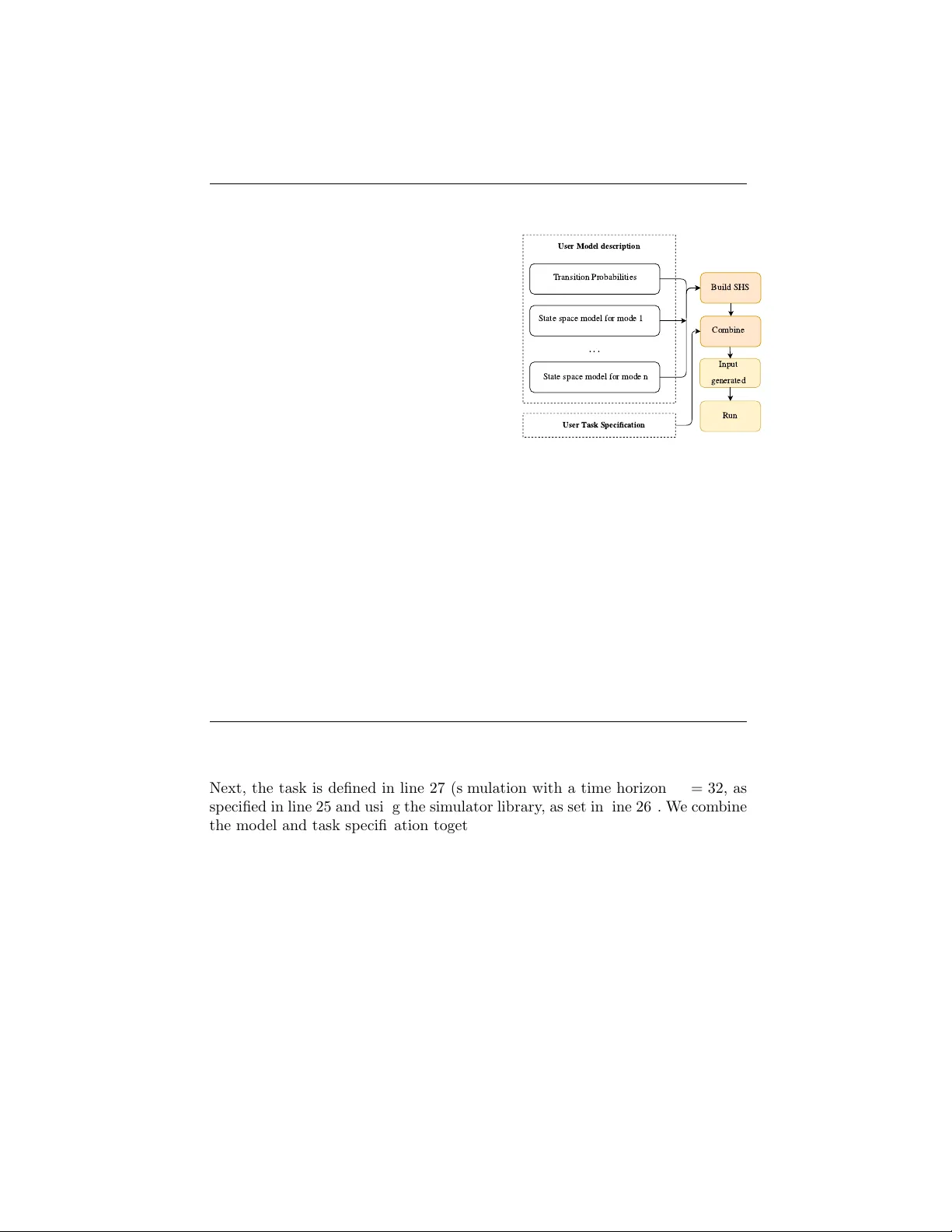
Sto cHy : automated v erification and syn thesis of sto c hastic pro cesses Nathalie Cauc hi 1 , Kurt Degiorgio 2 , and Alessandro Abate 1 1 Departmen t of Computer Science, Univ ersit y of Oxford, United Kingdom, { nathalie.cauchi, alessandro.abate } @cs.ox.ac.uk , 2 Diffblue Ltd, United Kingdom, kurt.degiorgio@diffblue.com Abstract. StocHy is a soft w are tool for the quan titativ e analysis of discrete-time sto chastic hybrid systems ( shs ). StocHy accepts a high-lev el description of sto c hastic models and constructs an equiv alent shs mo del. The to ol allows to (i) sim ulate the shs evolution o ver a giv en time hori- zon; and to automatically construct formal abstractions of the shs . Ab- stractions are then emplo yed for (ii) formal verification or (iii) con trol (p olicy , strategy) syn thesis. Sto cHy allows for modular mo delling, and has separate simulation, verification and syn thesis engines, which are implemen ted as indep endent libraries. This allows for libraries to b e eas- ily used and for extensions to b e easily built. The to ol is implemented in c++ and employs manipulations based on v ector calculus, the use of sparse matrices, the symbolic construction of probabilistic kernels, and m ulti-threading. Exp erimen ts sho w StocHy ’s mark edly improv ed p er- formance when compared to existing abstraction-based approaches: in particular, StocHy beats state-of-the-art tools in terms of precision (ab- straction error) and computational effort, and finally attains scalability to large-sized models (12 contin uous dimensions). Sto cHy is a v ailable at www.gitlab.com/natchi92/StocHy . 1 In tro duction Sto chastic hybrid systems ( shs ) are a ric h mathematical mo delling framework capable of describing systems with complex dynamics, where uncertaint y and h ybrid (that is, b oth contin uous and discrete) components are relev an t. Whilst earlier instances of shs hav e a long history , shs proper ha v e b een thoroughly in v estigated only from the mid 2000s, and hav e b een most recen tly applied to the study of complex systems, both engineered and natural. Amongst the first class, shs ha v e been used for mo delling and analysis of smart grids [27], automation of medical devices [3], a vionics [7], prognostics and health managemen t [29]. Ho w ev er, a wider adoption of shs in real-w orld applications is st ymied b y a few factors: (i) the complexit y associated with mo delling shs ; (ii) the gener- alit y of their mathematical framework, which requires an arsenal of adv anced and div erse techniques to analyse them; and (iii) the undecidabilit y of v erifi- cation/syn thesis problems ov er shs and the curse of dimensionality asso ciated with their appro ximations. 2 Cauc hi et al. This pap er introduces a new softw are tool - StocHy - whic h is aimed at sim- plifying both the mo delling of shs and their analysis, and targets the wider adoption of shs by non-exp ert users. With fo cus on the three limiting factors ab o ve, Sto cHy allows to describ e shs by parsing or extending w ell-kno wn and -used state-space mo dels and generates a standard shs mo del automatically and formats it to be analysed. StocHy can (i) p erform v erification tasks, e.g., compute the probability of sta ying within a certain region of the state space from a giv en set of initial conditions; (ii) automatically synthesise policies (strategies) max- imising this probability , and (iii) simulate the shs evolution o v er time. Sto cHy is implemen ted in c++ and mo dular making it both extendible and p ortable. Related work. There exist only a few tools that can handle (classes of ) shs . Of muc h inspiration for this contribution, f aust 2 [26] generates abstractions for uncoun table-state discrete-time stochastic processes, natively supporting shs mo d- els with a single discrete mo de and finite actions, and p erforms verification of reac habilit y-lik e prop erties and corresp onding syn thesis of p olicies. f aust 2 is na ¨ ıv ely implemen ted in ma tlab and lac ks in scalabilit y to large models. mod- est toolset [17] allo ws to mo del and to analyse classes of con tin uous-time shs , particularly probabilistic hybrid automata ( pha ) that combine probabilis- tic discrete transitions with deterministic ev olution of the contin uous v ariables. The to ol for sto c hastic and dynamically coloured p etri nets ( sdcpn ) [12] sup- p orts comp ositional mo delling of pha and focuses on simulation via Mon te Carlo tec hniques. The existing tools highlight the need for a new softw are that allo ws for (i) straigh tforw ard and general shs mo delling construction and (ii) scalable automated analysis. Con tributions. The Sto cHy to ol newly enables – formal verific ation of shs via either of t w o abstraction tec hniques: • for discrete-time, contin uous-space mo dels with additiv e disturbances, and p ossibly with multiple discrete modes, w e emplo y formal abstrac- tions as general Marko v chains or Mark o v decision proces ses [26]; StocHy impro v es tec hniques in the f aust 2 to ol by simplifying the input mo del description, b y emplo ying sparse matrices to manipulate the transition probabilities and by reducing the computational time needed to generate the abstractions. • for mo dels with a finite n um b er of actions, we emplo y in terv al Mark o v decision pro cesses and the model c hec king framework in [21]; Sto cHy pro- vides a nov el abstraction algorithm allo wing for efficient computation of the abstract model, b y means of an adaptive and sequential refining of the underlying abstraction. W e sho w that we are able to generate sig- nifican tly smaller abstraction errors and to v erify mo dels with up to 12 con tin uous v ariables. – c ontr ol (strategy , p olicy) synthesis via formal abstractions, employing: • stochastic dynamic programming; Sto cHy exploits the use of symbolic k ernels. Sto cHy 3 • robust syn thesis using in terv al Mark o v decision processes; StocHy auto- mates the synthesis algorithm with the abstraction pro cedure and the temp oral property of in terest, and exploits the use of sparse matrices; – simulation of complex sto c hastic pro cesses, suc h as shs , b y means of Monte Carlo techniques; Sto cHy automatically generates statistics from the sim- ulations in the form of histograms, visualising the evolution of b oth the con tin uous random v ariables and the discrete mo des. This con tribution is structured as follo ws: Sec. 2 crisply presents the theoreti- cal underpinnings (modelling and analysis) for the tool. W e provide an ov erview of the implementation of Sto cHy in Sec. 3. W e highligh t features and use of Sto cHy by a set of experimental ev aluations in Sec. 4: w e provide four differ- en t case studies that highlight the applicability , ease of use, and scalability of Sto cHy . Details on executing all the case studies are detailed in this pap er and within a Wiki page that accompanies the Sto cHy distribution. 2 Theory: Mo dels, Abstractions, Simulations 2.1 Mo dels - Sto c hastic Hybrid Systems Sto cHy supp orts the modelling of the following general class of shs [1, 4]. Definition 1. A shs [4] is a discr ete-time mo del define d as the tuple H = ( Q , n, U , T x , T q ) , w here (1) – Q = { q 1 , q 2 , . . . , q m } , m ∈ N , r epr esents a finite set of mo des (lo c ations); – n ∈ N is the dimension of the c ontinuous sp ac e R n of e ach mo de; the hybrid state sp ac e is then given by D = ∪ q ∈Q { q } × R n ; – U is a c ontinuous set of actions, e.g. R v ; – T q : Q × D × U → [0 , 1] is a discr ete sto chastic kernel on Q given D × U , which assigns to e ach s = ( q , x ) ∈ D and u ∈ U , a pr ob ability distribution over Q : T q ( ·| s, u ) ; – T x : B ( R n ) × D × U → [0 , 1] is a Bor el-me asur able sto chastic kernel on R n given D × U , which assigns to e ach s ∈ D and u ∈ U a pr ob ability me asur e on the Bor el sp ac e ( R n , B ( R n )) : T x ( ·| s, u ) . In this mo del the discrete comp onen t takes v alues in a finite set Q of mo des (a.k.a. lo cations), each endow ed with a contin uous domain (the Euclidean space R n ). As suc h, a point s o ver the h ybrid state space D is pair ( q , x ), where q ∈ Q and x ∈ R n . The seman tics of transitions at any p oin t o v er a discrete time domain, are as follo ws: giv en a p oin t s ∈ D , the discrete state is chosen from T q , and dep ending on the selected mo de q ∈ Q the con tin uous state is updated according to the probabilistic la w T x . Non-determinism in the form of actions can affect b oth discrete and con tinuous transitions. 4 Cauc hi et al. R emark 1. A rigorous c haracterisation of shs can be found in [1], whic h in tro- duces a general class of mo dels with probabilistic resets and a hybrid actions space. Whilst in principle we can deal with general shs models, in the case stud- ies of this pap er w e fo cus on sp ecial instances, as described next. u t R emark 2 (Sp e cial instanc e). In Case Study 2 (see Sec. 4.2) w e lo ok at mo dels where actions are asso ciated to a deterministic selection of lo cations, namely T q : U → Q and U is a finite set of actions. u t R emark 3 (Sp e cial instanc e). In Case Study 4 (Section 4.4) w e consider non- linear dynamical mo dels with bilinear terms, whic h are characterised for an y q ∈ Q b y x k +1 = A q x k + B q u k + x k P v i =1 N q ,i u i,k + G q w k , where k ∈ N represents the discrete time index, A q , B q , G q are appropriately sized matrices, N q ,i represen ts the bilinear influence of the i − th input component u i , and w k = w ∼ N ( · ; 0 , 1) and N ( · ; η , ν ) denotes a Gaussian densit y function with mean η and cov ariance matrix ν 2 . This expresses the con tin uous k ernel T x : B ( R n ) × D × U → [0 , 1] as N ( · ; A q x + B q u + x v X i =1 N q ,i u i + F q , G q ) . (2) In Case Study 1-2-3 (Sec. 4.1-4.3), we lo ok at the sp ecial instance from [21], where the dynamics are autonomous (no actions) and linear: here T x is N ( · ; A q x + F q , G q ) , (3) where in Case Studies 1, 3 Q is a single element. u t Definition 2. A Markov de cision pr o c ess ( mdp ) [5] is a discr ete-time mo del define d as the tuple H = ( Q , U , T q ) , w here (4) – Q = { q 1 , q 2 , . . . , q m } , m ∈ N , r epr esents a finite set of mo des; – U is a finite set of actions; – T q : Q × Q × U → [0 , 1] is a discr ete sto chastic kernel that assigns, to e ach q ∈ Q and u ∈ U , a pr ob ability distribution over Q : T q ( ·| q , u ) . Whenev er the set of actions is trivial or a p olicy is syn thesised and used (cf. discussion in Sec. 2.2) the mdp reduces to a Marko v c hain ( mc ), and a k ernel T q : Q × Q → [0 , 1] assigns to eac h q ∈ Q a distribution ov er Q as T q ( ·| q ). Definition 3. A n interval Markov de cision pr o c ess ( imdp ) [24] extends the syn- tax of an mdp by al lowing for unc ertain T q , and is define d as the tuple H = ( Q , U , ˇ P , ˆ P ) , wher e (5) – Q and U ar e as in Def. 2; – ˇ P and ˆ P : Q × U × Q → [0 , 1] is a function that assigns to e ach q ∈ Q a lower (upp er) b ound pr ob ability distribution over Q : ˇ P ( ·| q , u ) ( ˆ P ( ·| q , u ) r esp e ctively). Sto cHy 5 F or al l q, q 0 ∈ Q and u ∈ U , it holds that ˇ P ( q 0 | q , u ) ≤ ˆ P ( q 0 | q , u ) and, X q 0 ∈Q ˇ P ( q 0 | q , u ) ≤ 1 ≤ X q 0 ∈Q ˆ P ( q 0 | q , u ) . Note that when ˇ P ( ·| q , u ) = ˆ P ( ·| q , u ) , the imdp r e duc es to the mdp with ˇ P ( ·| q , u ) = ˆ P ( ·| q , u ) = T q ( ·| q , u ) . 2.2 F ormal V erification and Strategy Syn thesis via Abstractions F ormal v erification and strategy syn thesis ov er shs are in general not decid- able [4, 28], and can b e tackled via quantitativ e finite abstractions. These are precise approximations that come in t w o main different fla v ours: abstractions in to mdp [4, 26] and into imdp [21]. Once the finite abstractions are obtained, and with focus on sp ecifications expressed in (non-nested) pctl or fragments of l tl [5], formal v erification or strategy syn thesis can b e p erformed via proba- bilistic mo del c hecking to ols, suc h as prism [20], storm [11], iscasMc [16]. W e o v erview next the t w o alternativ e abstractions, as implemen ted in Sto cHy . Abstractions in to Marko v decision pro cesses F ollowing [25], mdp are gen- erated by either (i) uniformly gridding the state space and computing an ab- straction error, which dep ends on the contin uit y of the underlying contin uous dynamics and on the chosen grid; or (ii) generating the grid adaptively and se- quen tially , by splitting the cells with the largest lo cal abstraction error until a desired global abstraction error is achiev ed. The tw o approaches display an in- tuitiv e trade-off, where the first in general requires more memory but less time, whereas the second generates smaller abstractions. Either w ay , the probability to transit from eac h cell in the grid into any other cell c haracterises the mdp matrix T q . F urther details can b e found in [26]. StocHy newly provides a c++ imple- men tation and employs sparse matrix representation and manipulation, in order to attain faster generation of the abstraction and use in formal v erification or strategy syn thesis. V erific ation via mdp (when the action set is trivial) is p erformed to c hec k the abstraction against non-nested, b ounded-un til sp ecifications in pctl [5] or c o- safe line ar temp or al lo gic ( csl tl ) [19]. Str ate gy synthesis via mdp is defined as follows. Consider, the class of determin- istic and memoryless Marko v strategies π = ( µ 0 , µ 1 , . . . ) where µ k : Q → U . W e compute the strategy π ? that maximises the probability of satisfying a formula, with algorithms discussed in [26]. Abstraction in to In terv al Mark ov decision pro cesses ( imdp ) is based on a pro cedure in [10] performed using a uniform grid and with a finite set of actions U (see Remark 2). Sto cHy newly provides the option to generate a grid using adaptiv e/sequen tial refinements (similar to the case in the paragraph ab o v e) [25], whic h is performed as follows: (i) define a required minimal maxim um abstraction error ε max ; (ii) generate a coarse abstraction using the Algorithm in [10] and compute the local error ε q that is associated to eac h abstract state q ; (iii) split 6 Cauc hi et al. all cells where ε q > ε max along the main axis of eac h dimension, and up date the probabilit y b ounds (and errors); and (iv) rep eat this pro cess un til ∀ q, ε q < ε max . V erific ation via imdp is run ov er properties in csl tl or bounded-L TL ( bl tl ) form using the imdp mo del c hecking algorithm in [21]. Synthesis via imdp [10] is carried out b y extending the notions of strategies of mdp to dep end on memory , that is on prefixes of paths. 2.3 Analysis via Monte Carlo sim ulations Mon te Carlo techniques generate numerical sampled tra jectories represen ting the ev aluation of a sto c hastic pro cess o v er a predetermined time horizon. Given a sufficien t n um b er of tra jectories, one can appro ximate the statistical properties of the solution process with a required confidence lev el. This approach has b een adopted for simulation of different t yp es of shs . [18] applies sequential Monte Carlo sim ulation to shs to reason ab out rare-ev en t probabilities. [12] performs Mon te Carlo sim ulations of classes of shs describ ed as Petri nets. [8] prop oses a metho dology for efficient Monte Carlo simulations of contin uous-time shs . In this work, w e analyse a shs model using Monte Carlo sim ulations following the approac h in [4]. Additionally , we generate histogram plots at eac h time step, pro viding further insigh t on the ev olution of the solution pro cess. 3 Ov erview of Sto cHy Installation StocHy is set up using the pro vided get dep file found within the distribution pack age, which will automatically install all the required dep en- dencies. The executable run.sh builds and runs Sto cHy . This basic installation setup has b een successfully tested on mac hines running Ubuntu 18.04.1 L TS GNU and Lin ux op erating systems. Input interface The user in teracts with Sto cHy via the main file and m ust sp ecify (i) a high-level description of the mo del dynamics and (ii) the task to b e performed. The description of model dynamics can take the form of a list of the transition probabilities b et w een the discrete mo des, and of the state-space mo dels for the contin uous v ariables in eac h mo de; alternativ ely , a description can b e obtained by sp ecifying a path to a ma tlab file con taining the mo del descrip- tion in state-space form together with the transition probability matrix. T asks can b e of three kinds (eac h admitting specific parameters): simulation, v erifica- tion, or syn thesis. The general structure of the input in terface is illustrated via an example in Listing 1.1: here the user is interested in simulating a shs with t w o discrete modes Q = { q 0 , q 1 } and t w o con tin uous v ariables ev olv e according to (3). The mo del is autonomous and has no control actions. The relationship b et ween the discrete modes is defined by a fixed transition probabilit y (line 1). The ev olution of the contin uous dynamics are defined in lines 2-14. The initial condition for b oth the discrete mo des and the con tin uous v ariables are set in lines 16-21 (this is needed for simulation tasks). The equiv alent shs mo del is then set up b y instan tiating an ob ject of type shs t (line 23). Sto cHy 7 1 arma::mat Tq = { {0.4, 0.6},{0.7,0.3}}; // Transition probabilities 2 // Evolution of the continuous variables for each discrete mode 3 // First model 4 arma::mat Aq0 = {{0.5, 0.4},{0.2,0.6}}; 5 arma::mat Fq0 = { {0},{0}}; 6 arma::mat Gq0 = {{0.4,0},{0.3, 0.3}}; 7 ssmodels_t modelq0(Aq0, Fq0, Gq0); 8 // Second model 9 arma::mat Aq1 = {{0.6, 0.3},{0.1,0.7}}; 10 arma::mat Fq1 = { {0},{0}}; 11 arma::mat Gq1 = {{0.2,0},{0.1, 0}}; 12 ssmodels_t modelq1(Aq1,Fq1, Gq1); 13 std::vector models = 14 {modelq1,modelq2}; 15 // Set initial conditions 16 // Initial state q_0 17 arma::mat q_init = arma::zeros(1,1); 18 // Initial continuous variables 19 arma::mat x1_init = arma::ones(2,1); 20 exdata_t data(x1_init,q_init); 21 // Build shs 22 shs_t mySHS(Tq,models,data); 23 // Time horizon 24 int K = 32; 25 // Task definition (1 = simulator, 2 = faust^2, 3 = imdp) 26 int lb = 1; 27 taskSpec_t mySpec(lb,K); 28 // Combine 29 inputSpec_t myInput(mySHS,mySpec); 30 // Perform task 31 performTask(myInput); Listing 1.1: Description of main file for simulating a shs consisting of t w o discrete mo des and t wo con tin uous v ariables evolving according to (2). I n p u t g e n e r a t e d U s e r M o de l de s c r ip t io n T r a n s i t i o n P r o b a b i l i t i e s S t a t e s p a c e m o d e l f o r m o d e 1 S t a t e s p a c e m o d e l f o r m o d e n . . . B u i l d S H S U s e r T a s k Spe c i fi c a t io n C o m b i n e R u n Next, the task is defined in line 27 (simulation with a time horizon K = 32, as sp ecified in line 25 and using the sim ulator library , as set in line 26). W e com bine the mo del and task specification together in line 29. Finally , Sto cHy carries out the sim ulation using the function performTask (line 31). Mo dularit y Sto cHy comprises independent libraries for differen t tasks, namely (i) f aust 2 , (ii) imdp , and (iii) sim ulator. Each of the libraries is separate and dep ends only on the model structure that has b een entered. This allows for seamless extensions of individual sub-mo dules with new or existing tools and metho ds. The function performTask acts as multiplexer for calling any of the libraries dep ending on the input model and task sp ecification. Data structures Sto cHy makes use of m ultiple techniques to minimise com- putational o v erhead. It emplo ys v ector algebra for efficien t handling of linear op erations, and whenever p ossible it stores and manipulates matrices as sparse 8 Cauc hi et al. structures. It uses the linear algebra library Armadillo [22, 23], whic h applies m ulti-threading and a sophisticated expression ev aluator that has b een shown to sp eed up matrix manipulations in c++ when compared to other libraries. f aust 2 based abstractions define the underlying kernel functions symbolically using the library GiNaC [6], for easy ev aluation of the sto c hastic k ernels. Output in terface W e pro vide outputs as text files for all three libraries, which are stored within the resul ts folder. W e also pro vide additional python scripts for generating plots as needed. F or abstractions based on f aust 2 , the user has the additional option to export the generated mdp or mc to prism format, to interface with the popular model c heck er [20] ( Sto cHy prompts the user this option follo wing the completion of the v erification or synthesis task). As a future extension, w e plan to exp ort the generated abstraction mo dels to the mo del c hec k er storm [11] and to the mo delling format jani [9]. 4 Sto cHy : Exp erimental Ev aluation W e apply StocHy on four differen t case studies highlighting differen t mo dels and tasks to b e p erformed. All the experiments are run on a standard laptop, with an In tel Core i7-8550U CPU at 1.80GHz × 8 and with 8 GB of RAM. 4.1 Case Study 1 - F ormal V erification W e consider the shs mo del first presen ted in [2]. The mo del tak es the form of (1), and has one discrete mo de and t w o contin uous v ariables representing the lev el of CO 2 ( x 1 ) and the am bien t temp erature ( x 2 ), resp ectiv ely . The con tin uous v ariables evolv e according to x 1 ,k +1 = x 1 ,k + ∆ V ( − ρ m x 1 ,k + % c ( C out − x 1 ,k )) + σ 1 w k , (6) x 2 ,k +1 = x 2 ,k + ∆ C z ( ρ m C pa ( T set − x 2 ,k ) + % c R ( T out − x 2 ,k )) + σ 2 w k , where ∆ the sampling time [ min ], V is the volume of the zone [ m 3 ], ρ m is the mass air flow pumped inside the ro om [ m 3 /min ], % c is the natural drift air flo w [ m 3 /min ], C out is the outside C O 2 lev el [ ppm/min ], T set is the desired temp erature [ o C ], T out is the outside temp erature [ ◦ C /min ], C z is the zone capacitance [ J m 3 / ◦ C ], C pa is the sp ecific heat capacity of air [ J / ◦ C ], R is the resistance to heat transfer [ ◦ C /J ], and σ ( · ) is a v ariance term asso ciated to the noise w k ∼ N (0 , 1). W e are in terested in v erifying whether the con tinuous v ariables remain within the safe set X saf e = [405 , 540] × [18 , 24] ov er 45 minutes ( K = 3). This property can b e enco ded as a bl tl property , ϕ 1 :=  ≤ K X saf e , where  is the “ always ” temp oral op erator considered ov er a finite horizon. The semantics of bl tl is defined ov er finite traces, denoted b y ζ = { ζ j } K j =0 . A trace ζ satisfies ϕ 1 if ∀ j ≤ K, ζ j ∈ X saf e , and we quan tify the probabilit y that traces generated by the shs satisfy ϕ 1 . Sto cHy 9 Case study 1: Listings explaining task sp ecification for (a) f a ust 2 and (b) imdp 1 // Dynamics definition 2 shs_t myShs( ’../CS1.mat’ ); 3 // Specification for FAUST^2 4 // safe set 5 arma::mat safe = {{18,24},{18,24}}; 6 // max error 7 double eps = 1; 8 // grid type 9 // (1 = uniform, 2 = adaptive) 10 int gridType = 1; 11 // time horizon 12 int K = 3; 13 // task and property type 14 // (1 = verify safety , 2 = verify reach-avoid, 15 // 3 = safety synthesis, 4 = reach-avoid synthesis) 16 int p = 1; 17 // library (1 = simulator, 2 = faust^2, 3 = imdp) 18 int lb = 2; 19 // task specification 20 taskSpec_t mySpec(lb,K,p,safe,eps,gridType); Listing 1.2: (a) f aust 2 // Dynamics definition shs_t myShs( ’../CS1.mat’ ); // Specification for IMDP // safe set arma::mat safe = {{18,24},{18,24}}; // grid size for each dimension arma::mat grid = {{0.0845,0.0845}}; // relative tolerance arma::mat reft = {{1,1}}; // time horizon int K = 3; // task and property type // (1 = verify safety , 2 = verify reach-avoid, // 3 = safety synthesis, 4 = reach-avoid synthesis) int p = 1; // library (1 = simulator, 2 = faust^2, 3 = imdp) int lb = 3; // task specification taskSpec_t mySpec(lb,K,p,safe,grid,reft); Listing 1.3: (b) imdp When tac kled with the metho d based on f a ust 2 that hinges on the compu- tation of Lipschitz constants, this verification task is n umerically tric ky , in view of difference in dimensionalit y of the range of x 1 and x 2 within the safe set X saf e and the v ariance asso ciated with each dimension G q 0 = [ σ 1 0 0 σ 2 ] = [ 40 . 096 0 0 0 . 511 ]. In order to mitigate this, w e rescale the state space so all the dynamics evolv e in a comparable range and also apply the abstraction based on imdp . More pre- cisely (this is done externally to Sto cHy ), we consider an affine map x = J y with J = [ 22 . 5 0 0 1 ], whic h results in the safe set X saf e to [18 , 24] 2 and in G q 0 = [ 1 . 782 0 0 0 . 511 ]. Consequently , the generated cell partitions are more uniform, with finer partitioning along x 2 . The dynamics of the new state space are pro vided in the file cs1.ma t . Implemen tation Sto cHy provides tw o v erification metho ds, one based on f a ust 2 and the second based on imdp . W e parse the mo del from file cs1.ma t (see line 2 of Listings 1.2(a) and 1.3(b), corresp onding to the tw o methods). cs1.ma t sets parameter v alues to (6) and uses a ∆ = 15 [ min ]. As anticipated, we emplo y b oth tec hniques ov er the same model description: 10 Cauc hi et al. – for f aust 2 w e sp ecify the safe set ( X saf e ), the maximum allow able error, the grid type (whether uniform or adaptive grid), the time horizon, together with the type of property of in terest (safety or reac h-a v oid). This is carried out in lines 5-21 in Listing 1.2(a). – for the imdp metho d, we define the safe set ( X saf e ), the grid size, the relative tolerance, the time horizon and the prop ert y t ype. This can be done by defining the task sp ecification using lines 5-21 in Listing 1.3 (b). Finally , to run either of the metho ds on the defined input mo del, w e com- bine the mo del and the task sp ecification using inputSpec t myInput(myShs,mySpec) , then run the command performTask(myInput) . The v erification results for b oth methods are stored in the resul ts directory: – for f aust 2 , Sto cHy generates four text files within the resul ts folder: represent a tive points.txt contains the partitioned state space; tran- sition ma trix.txt consists of the transition probabilities of the generated abstract mc ; pr oblem solution.txt contains the sat probability for eac h state of the mc ; and e.txt stores the global maximum abstraction error. – for imdp , StocHy generates three text files in the same folder: stepsmin.txt stores ˇ P of the abstract imdp ; stepsmax.txt stores ˆ P ; and solution.txt con tains the sat probabilit y and the errors ε q for eac h abstract state q . T o ol Impl. |Q| Time Error Metho d Platform [states] [s] ε max f aust 2 ma tlab 576 186.746 1 f aust 2 c++ 576 51.420 1 imdp c++ 576 87.430 0.236 f aust 2 ma tlab 1089 629.037 1 f aust 2 c++ 1089 78.140 1 imdp c++ 1089 387.940 0.174 f aust 2 ma tlab 2304 2633.155 1 f aust 2 c++ 2304 165.811 1 imdp c++ 2304 1552.950 0.121 f aust 2 ma tlab 3481 7523.771 1 f aust 2 c++ 3481 946.294 1 imdp c++ 3481 3623.090 0.098 f aust 2 ma tlab 4225 10022.850 0.900 f aust 2 c++ 4225 3313.990 0.900 imdp c++ 4225 4854.580 0.089 T able 1: Case study 1: Comparison of v erification results for ϕ 1 when using f aust 2 vs imdp . Fig. 1: Case study 1: Lo w er b ound probabilit y of satisfying ϕ 1 gener- ated using imdp with 3481 states. Outcomes W e p erform the v erification task using b oth f a ust 2 and imdp , o ver differen t sizes of the abstraction grid. W e employ uniform gridding for both metho ds. W e further compare the outcomes of Sto cHy against those of the f aust 2 to ol, which is implemen ted in ma tlab [26]. Note that the imdp con- sists of |Q| + 1 states, where the additional state is the sink state q u = D \ X saf e . Sto cHy 11 gr e en purple gr e en -1 0 1 -1 0 1 (a) (b) (c) Fig. 2: Case study 2: (a) Gridded domain together with a sup erimp osed sim- ulation of tra jectory initialised at ( − 0 . 5 , − 1) within q 0 , under the synthesised optimal switching strategy π ∗ . Low er probabilities of satisfying ϕ 2 for mo de q 0 (b) and for mo de q 1 (c), as computed b y Sto cHy . The results are sho wn in T able 1. W e saturate (conserv ativ e) errors output that are greater than 1 to this v alue. W e show the probability of satisfying the for- m ula obtained from imdp for a grid size of 3481 states in Fig. 1 – similar prob- abilities are obtained for the remaining grid sizes. As eviden t from T able 1, the new imdp metho d outperforms the approach using f aust 2 in terms of the maxim um error asso ciated to the abstraction ( f aust 2 generates an abstraction error < 1 only with 422 5 states). Comparing the f a ust 2 within StocHy and the original f aust 2 implemen tation (running in ma tlab ), Sto cHy offers computa- tional speed-up for the same grid size. This is due to the faster computation of the transition probabilities, through Sto cHy ’s use of matrix manipulations. f aust 2 within StocHy also simplifies the input of the dynamical mo del descrip- tion: in the original f aust 2 implemen tation, the user is ask ed to manually input the sto c hastic kernel in the form of sym bolic equations in a ma tlab script. This is not required when using Sto cHy , whic h automatically generates the underlying sym b olic k ernels from the input state-space mo del descriptions. 4.2 Case Study 2 - Strategy Synthesis W e consider a stochastic process with t w o modes Q = { q 0 , q 1 } , whic h con tinu- ously ev olv es according to (3) with A q 0 =  0 . 43 0 . 52 0 . 65 0 . 12  , G q 0 =  1 0 . 1 0 0 . 1  , A q 0 =  0 . 65 0 . 12 0 . 52 0 . 43  , G q 1 =  0 . 2 0 0 0 . 2  , F q i =  0 0  , and i ∈ { 0 , 1 } . Consider the con tinuous domain shown in Fig.2a ov er b oth dis- crete lo cations. W e plan to syn thesise the optimal switc hing strategy π ? that maximises the probability of reaching the gr e en region, whilst av oiding the pur- ple one, o v er an unbounded time horizon, giv en an y initial condition within the domain. This requirement can b e expressed with the l tl formula, ϕ 2 := ( ¬ pur ple ) U g r een, where U is the “ until ” temp oral op erator, and the atomic 12 Cauc hi et al. prop ositions { pur ple, g r een } denote regions within the set X = [ − 1 . 5 , 1 . 5] 2 , as sho wn in Fig. 2a. Implemen tation W e define the mo del dynamics follo wing lines 3-14 in List- ing 1.1, while w e use Listing 1.3 to specify the synthesis task and together with its asso ciated parameters. The l tl prop erty ϕ 2 is ov er an un b ounded time hori- zon, which leads to employing the imdp metho d for synthesis (recall that the f aust 2 implemen tation can only handle time-b ounded prop erties, and its ab- straction error monotonically increases with the time horizon of the formula). In order to enco de the task we set the v ariable safe to corresp ond to X the grid size to 0 . 12 and the relative tolerance to 0 . 06 along b oth dimensions (cf. lines 5-10 in Listing 1.3). W e set the time horizon K = -1 to represent an un- b ounded time horizon, let p = 4 to trigger the syn thesis engine o ver the giv en sp ecification and mak e lb = 3 to use imdp metho d (cf. lines 12-19 in List- ing 1.3). This task sp ecification partitions the set X into the underlying imdp via uniform gridding. Alternativ ely , the user has the option to make use of the adaptiv e-sequen tial algorithm b y defining a new v ariable eps max whic h charac- terise the maxim um allo wable abstraction error and then sp ecify the task using taskSpec t mySpec(lb,K,p,boundary,eps max,grid,rtol); . Next, w e define t w o files ( phi1 .txt and phi2.txt ) containing the coordinates within the grid- ded domain (see Fig.2a) asso ciated with the atomic prop ositions purple and gr e en , resp ectiv ely . This allo ws for automatic lab elling of the state-space ov er whic h syn thesis is to be p erformed. Running the main file, Sto cHy generates a Solution.txt file within the resul ts folder. This con tains the syn thesised π ? p olicy , the lo w er b ound for the probabilities of satisfying ϕ 2 , and the lo cal errors ε q for an y region q . Outcomes The case study generates an abstraction with a total of 2410 states, a maximum probabilit y of 1, a maxim um abstraction error of 0.21, and it requires a total time of 1639.3 [s]. In this case, we witness a slightly larger abstraction error via the imdp metho d then in the previous case study . This is due the non- diagonal co v ariance matrix G q 0 whic h in troduces a rotation in X within mode q 0 . When lab elling the states asso ciated with the regions pur pl e and gr een , an additional error is introduced due to the ov er- and under-approximation of states associated with eac h of the tw o regions. W e further sho w the sim ulation of a tra jectory under π ? with a starting p oin t of ( − 0 . 5 , − 1) in q 0 , within Fig.2a. 4.3 Case Study 3 - Scaling in Contin uous Dimension of Mo del W e now fo cus on the contin uous dynamics by considering a sto c hastic pro cess with Q = { q 0 } (single mo de) and dynamics ev olving according to (3), charac- terised b y A q 0 = 0 . 8 I d , F q 0 = 0 d and G q 0 = 0 . 2 I d , where d corresponds to the n um b er of con tin uous v ariables. W e are interested in c hec king the l tl sp ecifica- tion ϕ 3 :=  X saf e , where X saf e = [ − 1 , 1] d , as the contin uous dimension d of the mo del v aries. Here “  ” is the “ always ” temp oral op erator and a trace ζ satisfies ϕ 3 if ∀ k ≥ 0 , ζ k ∈ X saf e . In view of the focus on scalabilit y for this Case Study Sto cHy 13 Dimensions 2 3 4 5 6 7 8 9 10 11 12 [d] |Q| 4 14 30 62 126 254 510 1022 2046 4094 8190 [states] Time taken 0.004 0.06 0.21 0.90 4.16 19.08 79.63 319.25 1601.31 5705.47 21134.23 [s] Error 4.15e-5 3.34e-5 2.28e-5 9.70e-5 8.81e-6 1.10e-6 2.95e-6 4.50e-7 1.06e-7 4.90e-8 4.89e-8 ( ε max ) T able 2: Case study 3: V erification results of the imdp -based approach o v er ϕ 3 , for v arying dimension d of the sto c hastic process. 3, we disregard discussing the computed probabilities, whic h we instead co v ered in Section 4.1. Implemen tation Similar to Case Study 2, w e follow lines 3-14 in Listing 1.1 to define the mo del dynamics, while we use Listing 1.3 to sp ecify the v erification task using the imdp metho d. F or this example, we emplo y a uniform grid having a grid size of 1 and relativ e tolerance of 1 for each dimension (cf. lines 5-10 in Listing 1.3). W e set K = -1 to represen t an unbounded time horizon, p = 1 to p erform verification o ver a safety property and lb = 3 to use the imdp metho d (cf. lines 12-19 in Listing 1.3). In T able 2 w e list the n umber of states required for eac h dimension, the total computational time, and the maximum error asso ciated with eac h abstraction. Outcomes F rom T able 2 we can deduce that by emplo ying the imdp metho d within Sto cHy , the generated abstract mo dels hav e manageable state spaces, thanks to the tight error b ounds that is obtained. Notice that since the num- b er of cells p er dimension is increased with the dimension d of the mo del, the asso ciated abstraction error ε max is decreased. The small error is also due to the underlying contractiv e dynamics of the pro cess. This is a key fact leading to scalability ov er the contin uous dimension d of the mo del: Sto cHy displays a significant improv emen t in scalability o v er the state of the art [26] and al- lo ws abstracting sto c hastic mo dels with relev an t dimensionality . F urthermore, Sto cHy is capable to handle sp ecifications ov er infinite horizons (such as the considered until form ula). 4.4 Case Study 4 - Sim ulations F or this last case study , w e refer to the C O 2 mo del describ ed in Case Study 1 (Sec. 4.1). W e extend the C O 2 mo del to capture (i) the effect of o ccupan ts leaving or en tering the zone within a time step (ii) the op ening or closing of the windows in the zone [2]. ρ m is no w a con trol input and is an exogenous signal. This can b e describ ed as a shs comprising tw o-dimensional dynamics, o v er discrete mo des in the set { q 0 = ( E , C ) , q 1 = ( F , C ) , q 2 = ( F , O ) , q 3 = ( E , O ) } describing p ossible configurations of the room (empt y (E) or full (F), and with windows op en (O) or closed (C)). A mc represen ting the discrete modes and their dynamics is in Figure 3a. The con tin uous v ariables ev olv e according to Eqn. (6), which now 14 Cauc hi et al. captures the effect of switc hing b et ween discrete modes, as x 1 ,k +1 = x 1 ,k + ∆ V ( − ρ m x 1 ,k + % o,c ( C out − x 1 ,k )) + 1 F C occ,k + σ 1 w k , (7) x 2 ,k +1 = x 2 ,k + ∆ C z ( ρ m C pa ( T set − x 2 ,k ) + % o,c R ( T out − x 2 ,k )) + 1 F T occ,k + σ 2 w k , where the additional terms are: % ( · ) is the natural drift air flo w that changes dep ending whether the windo w is open ( % o ) or closed ( % c ) [ m 3 /min ]; C occ is the generated C O 2 lev el when the zone is o ccupied (it is m ultiplied b y the indicator function 1 F ) [ ppm/min ]; T occ is the generated heat due to occupants [ ◦ C /min ], whic h couples the dynamics in (7) as T occ,k = v x 1 ,k + ~ . q 1 =(F,C) q 2 =(F,O) q 0 =(E,C) q 3 =(E,O) 0 . 25 0 . 15 0 . 1 0 . 75 0 . 65 0 . 4 0 . 4 0 . 6 0 . 6 0 . 1 (a) 0 5 10 15 20 25 30 0 . 4 0 . 6 0 . 8 1 Time steps Control Signal ( ρ m ) (b) Fig. 3: Case study 4: (a) mc for the discrete mo des of the C O 2 mo del and (b) input con trol signal. 1 // Number of simulations 2 int monte = 5000; 3 // Initial continuous variables 4 arma::mat x_init = arma::zeros(2,monte); 5 // Initialise random generators 6 std::random_device rand_dev; 7 std::mt19937 generator(rand_dev()); 8 // Define distributions 9 std::normal_distribution< double > d1{450,25}; 10 std::normal_distribution< double > d2{17,2}; 11 for (size_t i = 0; i < monte; ++i) 12 { 13 x_init(0,i) = d1(generator); 14 x_init(1,i) = d2(generator); 15 } 16 // Initial discrete mode q_0 = (E,C) 17 arma::mat q_init = arma::zeros(1,monte); 18 // Definition of control signal 19 // Read from .txt/.mat file or define here 20 arma::mat u =readInputSignal( "../u.txt" ); 21 //Combining 22 exdata_t data(x_init,u,q_init); Listing 1.4: Case study 4: Definition of intial conditions for sim ulation Implemen tation The provided file cs4.ma t sets the v alues of the parameters in (7) and con tains the transition probability matrix representing the relation- ships b et w een discrete mo des. W e select a sampling time ∆ = 15 [ min ] and sim ulate the evolution of this dynamical model ov er a fixed time horizon K = 8 hours (i.e. 32 steps) with an initial CO 2 lev el x 1 ∼ N (450 , 25) [ ppm ] and a Sto cHy 15 0 5 10 15 20 25 30 380 400 Time steps x 1 (a) 0 5 10 15 20 25 30 18 18 . 5 19 19 . 5 20 Time steps x 2 (b) 0 5 10 15 20 25 30 (E,C) (F,C) (F,O) (E,O) Time steps (c) (d) (e) (f ) Fig. 4: Case study 4: Sim ulation single traces for con tinuous v ariables (a) x 1 , (b) x 2 and discrete modes (c) q . Histogram plots with resp ect to time step for (d) x 1 , (e) x 2 and discrete mo des (f ) q . temp erature lev el of x 2 ∼ N (17 , 2) [ ◦ C ]. W e define the initial conditions us- ing Listing 1.4. Line 2 defines the num b er of Mon te Carlo simulations using by the v ariable monte and sets this to 5000. W e instantiate the initial v alues of the con tin uous v ariables using the term x init , while we set the initial discrete mo de using the v ariable q init . This is done using lines 4-17 which defines inde- p enden t normal distribution for eac h of the contin uous v ariable from whic h we sample 5000 p oin ts for eac h of the contin uous v ariables and defines the initial discrete mode to q 0 = ( E , C ). W e define the control signal ρ m in line 20, by parsing the u.txt whic h contains discrete v alues of ρ m for eac h time step (see Fig. 3b). Once the mo del is defined, w e follow Listing 1.1 to p erform the sim- ulation. The simulation engine also generates a python script, simPlots.py , whic h giv es the option to visualise the sim ulation outcomes offline. Outcomes The generated sim ulation plots are shown in Fig. 4, whic h depicts: (i) a sample trace for each contin uous v ariable (the evolution of x 1 is shown in Fig. 4a, x 2 in Fig. 4b) and for the discrete mo des (see Fig. 4c); and (ii) histograms depicting the range of v alues the contin uous v ariables can be in during eac h time step and the associated coun t (see Fig. 4d for x 1 and Fig. 4e for x 2 ); and a histogram sho wing the likelihoo d of being in a discrete mode within each time step (see Fig. 4f). The total time taken to generate the simulations is 48.6 [s]. 5 Conclusions and Extensions W e ha v e presented Sto cHy , a new softw are to ol for the quantitativ e analysis of sto c hastic h ybrid systems. There is a plethora of en ticing extensions that we are planning to explore. In the short term, we in tend to: (i) interface with other mo del c hec king to ols such as storm [11] and the modest toolset [15]; (ii) 16 Cauc hi et al. em b ed algorithms for p olicy refinemen t, so w e can generate p olicies for mo dels ha ving n umerous con tin uous input v ariables [14]. In the longer term, w e plan to extend StocHy such that (i) it emplo ys a graphical user-in terface; (i) it ma y allo w analysis of contin uous-time shs ;and (iii) it mak es use of data structures suc h as m ulti-terminal binary decision diagrams [13] to reduce the memory requirements during the construction of the abstract mdp or imdp . Ac kno wledgemen ts The author’s would also like to thank Sadegh Soudjani, Sofie Haesaert, Luca Lauren ti, Morteza Lahijanian and Vira j Brian Wijesuriy a. This w ork is in part funded b y the Alan T uring Institute, UK, and by Malta’s ENDEA V OUR Scholarships Sc heme. References 1. Abate, A., Prandini, M., Lygeros, J., Sastry , S.: Probabilistic reachabilit y and safet y for controlled discrete time stochastic h ybrid systems. Automatica 44 (11), 2724–2734 (2008) 2. Abate, A.: F ormal v erification of complex systems: mo del-based and data-driven metho ds. In: Proceedings of the 15th A CM-IEEE In ternational Conference on F or- mal Methods and Models for System Design, MEMOCODE 2017, Vienna, Austria, Septem b er 29 - Octob er 02, 2017. pp. 91–93 (2017) 3. Abate, A., Blom, H., Cauchi, N., Haesaert, S., Hartmanns, A., Lesser, K., Oishi, M., Siv aramakrishnan, V., Soudjani, S., V asile, C.I., Vinod, A.P .: ARCH-COMP18 category rep ort: Sto c hastic mo delling. EPiC Series in Computing 54 , 71 – 103 (2018) 4. Abate, A., Kato en, J.P ., Lygeros, J., Prandin, M.: Approximate mo del chec king of sto c hastic h ybrid systems. European Journal of Con trol 16 (6), 624–641 (2010) 5. Baier, C., Katoen, J.P .: Principles of mo del c hecking. MIT press (2008) 6. Bauer, C., F rink, A., Kreck el, R.: In troduction to the GiNaC framework for sym- b olic computation within the C++ programming language. Journal of Symbolic Computation 33 (1), 1–12 (2002) 7. Blom, H., J. Lygeros (Eds.): Sto c hastic Hybrid Systems: Theory and Safet y Crit- ical Applications. No. 337 in Lecture Notes in Control and Information Sciences, Springer V erlag, Berlin Heidelb erg (2006) 8. Bouissou, M., Elmqvist, H., Otter, M., Benv eniste, A.: Efficien t monte carlo sim- ulation of sto c hastic hybrid systems. In: Pro ceedings of the 10 th International Mo delica Conference; March 10-12; 2014; Lund; Sw eden. pp. 715–725. No. 96, Link¨ oping Universit y Electronic Press (2014) 9. Budde, C.E., Dehnert, C., Hahn, E.M., Hartmanns, A., Junges, S., T urrini, A.: JANI: Quantitativ e mo del and to ol interaction. In: International Conference on T o ols and Algorithms for the Construction and Analysis of Systems. pp. 151–168. Springer (2017) 10. Cauc hi, N., Lauren ti, L., Lahijanian, M., Abate, A., Kwiatko wsk a, M., Cardelli, L.: Efficiency through uncertain ty: Scalable formal syn thesis for stochastic hybrid systems. In: 22nd A CM In ternational Conference on Hybrid Systems: Computation and Control (HSCC) (2019), arXiv: 1901.01576 11. Dehnert, C., Junges, S., Kato en, J.P ., V olk, M.: A storm is coming: A mo dern probabilistic model chec k er. In: Ma jumdar, R., Kun ˇ cak, V. (eds.) Computer Aided V erification. pp. 592–600. Springer International Publishing, Cham (2017) Sto cHy 17 12. Ev erdij, M.H., Blom, H.A.: Hybrid p etri nets with diffusion that hav e into- mappings with generalised sto c hastic hybrid pro cesses. In: Stochastic Hybrid Sys- tems, pp. 31–63. Springer (2006) 13. F ujita, M., McGeer, P .C., Y ang, J.Y.: Multi-terminal binary decision diagrams: An efficien t data structure for matrix represen tation. F ormal methods in system design 10 (2-3), 149–169 (1997) 14. Haesaert, S., Cauchi, N., Abate, A.: Certified policy syn thesis for general marko v decision pro cesses: An application in building automation systems. Performance Ev aluation 117 , 75–103 (2017) 15. Hahn, E.M., Hartmanns, A., Hermanns, H., Kato en, J.P .: A comp ositional mod- elling and analysis framework for sto chastic hybrid systems. F ormal Metho ds in System Design 43 (2), 191–232 (2013) 16. Hahn, E.M., Li, Y., Schew e, S., T urrini, A., Zhang, L.: iscasMc: A web-based probabilistic mo del c hec k er. In: Jones, C., Pihla jasaari, P ., Sun, J. (eds.) FM 2014: F ormal Methods. pp. 312–317. Springer International Publishing, Cham (2014) 17. Hartmanns, A., Hermanns, H.: The Mo dest T oolset: An Integrated En vironmen t for Quan titativ e Modelling and V erification, pp. 593–598. Springer Berlin Heidel- b erg, Berlin, Heidelberg (2014) 18. Krystul, J., Blom, H.A.: Sequen tial monte carlo sim ulation of rare ev en t probabilit y in sto chastic hybrid systems. IF A C Proceedings V olumes 38 (1), 176–181 (2005) 19. Kupferman, O., V ardi, M.Y.: Model chec king of safet y prop erties. F ormal Metho ds in System Design 19 (3), 291–314 (2001) 20. Kwiatk owsk a, M., Norman, G., Park er, D.: PRISM 4.0: V erification of probabilistic real-time systems. In: Gopalakrishnan, G., Qadeer, S. (eds.) Pro c. 23 rd In terna- tional Conference on Computer Aided V erification (CA V’11). LNCS, vol. 6806, pp. 585–591. Springer (2011) 21. Lahijanian, M., Andersson, S.B., Belta, C.: F ormal v erification and syn thesis for discrete-time sto c hastic systems. IEEE T ransactions on Automatic Control 60 (8), 2031–2045 (2015) 22. Sanderson, C., Curtin, R.: Armadillo: a template-based c++ library for linear algebra. Journal of Op en Source Softw are (2016) 23. Sanderson, C., Curtin, R.R.: A user-friendly hybrid sparse matrix class in C++. In: Mathematical Soft ware - ICMS 2018 - 6th In ternational Conference, South Bend, IN, USA, July 24-27, 2018, Pro ceedings. pp. 422–430 (2018) 24. ˇ Skulj, D.: Discrete time marko v chains with interv al probabilities. International journal of appro ximate reasoning 50 (8), 1314–1329 (2009) 25. Soudjani, S.E.Z.: F ormal Abstractions for Automated V erification and Synthesis of Sto chastic Systems. Ph.D. thesis, TU Delft (2014) 26. Soudjani, S.E.Z., Gev aerts, C., Abate, A.: F AUST 2 : F ormal Abstractions of Uncoun table-STate ST o c hastic pro cesses. In: T ACAS. vol. 15, pp. 272–286 (2015) 27. Stelec, M., Macek, K., Abate, A.: Modeling and simulation of a microgrid as a sto c hastic hybrid system. In: 2012 3 rd IEEE PES Innov ative Smart Grid T echnolo- gies Europ e (ISGT Europ e). pp. 1–9 (Oct 2012) 28. Summers, S., Lygeros, J.: V erification of discrete time sto c hastic h ybrid systems: A sto chastic reach-a void decision problem. Automatica 46 (12), 1951–1961 (2010) 29. Zhao, Z., Quan, Q., Cai, K.Y.: A health p erformance prediction metho d of large- scale stochastic linear hybrid systems with small failure probability . Reliabilit y Engineering & System Safety 165 , 74 – 88 (2017)