Electric Vehicle Charge Scheduling on Highway Networks from an Aggregate Cost Perspective

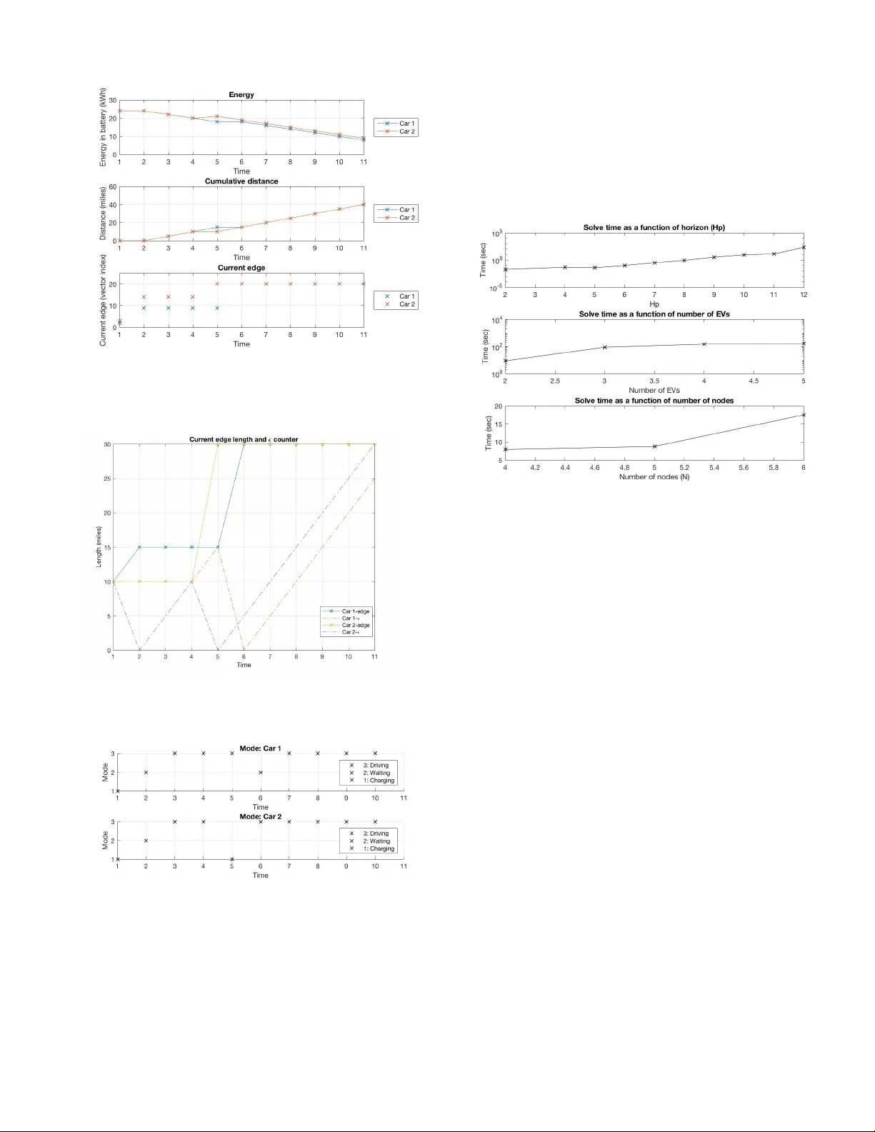
1 Electric V ehicle Char ge Scheduling on Highway Networks from an Aggre g ate Cost Perspecti v e Sean Anderson and V ineet Nair Abstract —In this paper , we attempt to optimally schedule the charging of long-range battery electric vehicles (BEVs) along highway networks, in order to minimize aggregate costs to the overall system consisting of utilities or electricity pro viders, station operators and other infrastructure, as well as EV users. Thus, we approach the problem from the perspectiv e of both customers (EV car owners), as well as charging station operators and utilities using a hybrid systems based formulation. I . I N T RO D U C T I O N A. Motivation The popularity of electric vehicles has been rising rapidly in recent years, driven mainly by the greater dri ving comfort, improv ed safety , cheaper maintenance and lower e xhaust emis- sions they offer . As battery and materials costs continue to decline and we transition tow ards cleaner , more div ersified and renew able electricity generation, the use of both plug-in hybrid and battery electric vehicles is likely to expand e ven more. Increased EV utilization rates also mean that we will need more sophisticated and effecti ve techniques to schedule the charging of both plug-in and battery electric vehicles in real- time, and allocate charging capacity or power in the most efficient manner . This is in order to minimize negati ve effects like congestion, long waiting times for customers and high infrastructure costs like uneven demands or loads for utilities and station operators. On a broader lev el, optimal EV charging will also play an important role in realizing smart grids of the future. B. Literatur e Review The work proposed thus far for EV scheduling has been focused on four areas: optimization with respect to load on power distribution networks [5], [9], [12], [13], [14], queuing models for input-output dynamics of char ging stations [1], [2], [6], [17], game-based approaches for trajectory optimization [2], [4], [8], and more traditional trajectory optimal control methods [3], [7], [10], [11], [15]. Note that po wer distrib ution problems either use game-based approaches or traditional optimal control methods but are considered distinct in their objectiv es: the former looks at power quality on netw orks whereas the latter has objective functions related to time or expected financial costs. The work done in power distribution considers the effect of EV charging on the grid, mainly with regard to base load. In this sense EVs are treated as dispatchable loads that can fill valleys during otherwise low demand. Other work has considered topological effects of char ging station power dra ws. The work described in [5] uses statistical estimation to predict future EV arriv als and the associated charging demands in order to perform load-shifting via model predicti ve control. [9] proposes a mean-field game-based approach for large EV populations. The objecti ve is to fill the ov ernight valle y in base load and does not consider EV routing. The work in [12] coordinates plug-in hybrid EVs (PHEV) in order to reduce system power losses, maximize load factor , and minimize load variance. A decentralized approach is proposed in [13] that focuses on load shifting via dispatch signals provided by a centralized authority . The issue of load shifting is considered in [14] with emphasis on circumventing load forecasting limi- tations. A locally optimal distrib uted approach is demonstrated. The work mentioned here focuses on optimization in the time domain–load shifting for valley filling throughout a day . Many different queuing model approaches hav e been pro- posed for optimal EV scheduling. These works generally focus on modeling the arriv al and departure/service rates of the EVs. While some approaches utilize probability theory as the foundation for the scheduling, others rely on optimization. The work in [1] presents a first-come first-served queuing model with arriv al rates corresponding to an exponential distribution and Poisson departure rates in a Markov chain. This does not account for location and path planning. The dynamics of the EV battery are not considered. A similar approach is shown in [2] where the objective is to minimize EV waiting time at charging stations. This mak es more considerations around path planning between nodes but limits the road network to a one-dimensional, unidirectional flow . [6] also minimizes EV waiting time using a similar queuing model. Theoretical bounds on waiting time are presented as well as a communication strategy (vehicle-to-charging station). A battery-swapping station approach in [17] utilizes queues and also defines probabilities around customer dissatisfaction. T rajectory optimization problems hav e been formulated for electric vehicle charging with an emphasis on finding effi- cient algorithms and sensible objectiv e functions. In [3] a hierarchical approach is proposed that considers power system network dynamics and battery dynamics. Giv en a fleet of EVs the highest le vel problem is station location. The pro visioning problem sits below this in which the number of chargers per station is allocated according to a queuing model and the giv en demand. The final layer consists of a global cost minimization. The work in [7] focuses on a graph theoretic framework for EV scheduling. The work exploits previous classical work done in path planning to reduce the complexity of scheduling EV char ging in lar ge networks. [10] details heuristic search algorithms for solving the EV -routing problem on a road network with charging stations located at specific nodes. A mixed approach is described in [11] whereby probabilistic tools, po wer distribution concerns, and an objectiv e function 2 formulated for routing efficiency are used. More specifically , the problem maximizes the station profits while maintaining a high equality of service. Finally , the work in [15] utilizes finite horizon and receding horizon approaches to consider the two cases of 1) a priori knowledge of all users and 2) new inputs (vehicles) to the system during the horizon for vehicle routing on a char ging network. The objecti ve function takes into consideration the customer’ s perspectiv e in an attempt to satisfy demand while keeping the cost low . Here a v ariable charging rate is implemented, which adds complexity to the required infrastructure and solution space but enables more interesting solutions. I I . C O N T R I B U T I O N S In this paper, we propose looking at the scheduling problem for EV charging from the perspective of minimizing aggr e gate costs to the system as a whole. This addresses an important null space in the literature since much of the previous work in this area has focused on optimizing the allocation of charging power with respect to only one of the players i.e. utilities, charging station operators, or customers. A lot of the past research has also focused on determin- ing optimal locations for char ging stations in a giv en area. Howe ver , in this paper, we take the station locations (i.e. the nodes) as a fixed parameter for a particular city or urban area’ s highway network. Instea d, we aim to design a central controller or algorithm that determines the optimal trajectory that an EV can take gi ven their starting position and desired destination, in a manner that maximizes benefits to all stakeholders inv olved. Furthermore, a great deal of effort has gone into minimizing losses to utilities and the grid - and utilizing EVs to provide services like load flattening, voltage and frequency regulation. Howe ver , we place more emphasis on the opportunity costs paid by customers as well, in terms of both time spent and physical degradation of their car batteries. Follo wing the prescribed route will also help alleviate range anxiety among users, and potentially contribute tow ards increased EV penetration. Additionally , this work defines a hybrid systems theoretic model and uses finite state machines to describe the dynamics of electric vehicles on a highway network under two dif ferent framew orks. The model is first described under a frame work that is more easily con verted into code. The second description allows for more thorough analysis of the model’ s properties. I I I . M O D E L The following model definitions and formulations formalize the Mixed Integer Quadratic Programming (MIQP) problem. A. Definitions and Notation T able I defines the basic terms that are used throughout the work. The remainder of the notation is defined in-text when first introduced. V ariable and Symbol Notes Car index c ∈ { 1 , ......, p } p = T otal no. of cars Time step k ∈ { 1 , ....., H p } H p = Prediction horizon Station index n ∈ { 1 , ....N } N = T otal no. of stations ν 0 Starting node for a car ν H p Ending node for a car d k Discrete trip distance counter  k Discrete local (edge) distance counter γ ∈ { 0 , 1 } Constrained input: at a node or on an edge y ∈ { 0 , 1 } Constrained input: charging or not E k Energy level of an EV at time k T ABLE I. D E FIN I T I ON S O F G E NE R A L N OTA T I ON B. Ke y Assumptions of F ormulation • All nodes or intersections in our highw ay network (rep- resented as a graph) have a charging station. • All EVs in our network ha ve identical battery energy lev el capacities and the same discharging power dynam- ics while driving. • All char ging stations in our network provide identical identical charging power profiles for all EV customers. C. Highway Network Model A highway network can be described as a connected graph G = ( V , E , A ) where V = { 1 , .., N } is a non-empty set of N nodes that represent road intersections and the potential loca- tion of a EV charging station, E is the set of edges representing the road segment lengths, and A is the adjacency matrix where a ii = 0 and a ij > 0 for all connected nodes i 6 = j . The adjacency matrix defines whether nodes are connected. For the set of edges, E , an entry e ij > 0 indicates the transition from node i to node j with a positiv e weight. Generally , a graph can be directed or undirected. Considering that the graph represents a highway , traffic is assumed to be able to flo w both ways without loss of generality . This can be generalized to cases with only one-way traf fic flo ws, because if ∃ e ij > 0 then and physically @ e j i > 0 , then e j i := 0 where the con vention is taken to be that only positiv e-valued edges can be trav ersed. Equiv alently , the zero-valued edges can be assigned to N aN or any placeholder value. Finally , the neighborhood of a node is defined where N i := { j | ( i, j ) ∈ E s.t. e ij > 0 } . The graph representation helps to formalize the work in notation but no nov el or extensi ve graph theory is used here. The network used in the simulations is presented in figure 1. It is included here to help moti vate the application of graph theory to the EV network. D. Costs for the Network C electr icity = N X n =1 H p − 1 X k =1 p X c =1 P elec k ( n ) ∗ y c k ∗ ( E k +1 − E k ) (1) Let P elec k ( n ) represent the electricity price (dollars/kWh) at a particular station n, as a function of location in the network and according to the time step k. The difference in energy 3 Fig. 1. Nodes represent charging stations. Node sizes correspond to station capacities. Edge weights represent distances in miles. Assume all nodes connected through two-way highways/roads results in an undirected graph when it is charging (i.e. when y k is true) is taken to be the amount of electricity , in kWh, that was just injected into the battery . This cost term then is in terms of dollars. W e originally considered including electricity costs using T ime-of-Use (TOU) rates as part of stations’ costs, as de- scribed in equation (III-D) above. Howe ver , we later decided against this since previous studies [8] have shown that elec- tricity costs are much smaller than costs associated with trav el times. Thus, we chose time minimization for customers as the dominant decision criterion, where tra velers choose the fastest feasible path while also satisfying the other constraints. C station = H p X k =1 N X n =1 ¯ C ∗ | sg n  U ( k , n ) S n − 0 . 5  | ∗ ( U ( k , n ) − S n ) (2) U ( k , n ) = p X c =1 y c k ( n ) (3) In order to avoid either excessiv e under or over -utilization of charging stations and ensure a uniform burden on all nodes across the network, we decided to penalize stations whenev er they use abov e or below 50% of their maximum rated capacity , as shown in (3). W e imposed a flat linear cost ¯ C on the difference between the current station utilization and the preferred capacity of that station S n . For simplicity , we defined station utilization U ( k , n ) in terms of the number of cars charging at a particular station n at any given time k . This can be easily computed by summing ov er the boolean variables y c k ( n ) in our logic FSM described in Section IV -C, as shown in (3) above. In general the following definition holds: sg n  U ( k , n ) S n − 0 . 5  =    1 , U ( k , n ) > 50% of S n 0 , U ( k , n ) = S n − 1 , U ( k , n ) < 50% of S n (4) E. Electric V ehicle Model The EV model is defined as three-mode finite-state machine (FSM) (Fig. 2). Namely , there is a charging mode, driving mode, and a waiting mode (at the charging station). The three piecewise-continuous states are the energy in the battery , the trip distance as a scalar v alue, and the current edge distance trav ersed. While less accurate than state of charge, the energy in the battery can be manipulated much more easily and with enough accuracy for the scheduling of trajectories. The dynamics of the battery are then a simplified version of Coulomb counting where the change in energy is a function of the power injected or consumed. Given ∂ E ∂ t := P ( t ) as the most basic form of Coulomb counting, let it be discretized under the one- step Euler to ∆ E := E k +1 − E k = P k ∗ T s , such that E k +1 = E k + P k ∗ T s where k denotes the discrete time and T s is the sampling time. This describes both the charge and discharge dynamics in this work. The charging power is a function of the energy in the battery as presented in [3] and the discharge power is a function of the incremental velocity , ˙ δ k . Thus the switched dynamics can defined on [ E , ¯ E ] where W aiting = β (1) , Charging = β (2) , and Driving = β (3) : E k +1 =    E k + P ( E k ) T s , β (1) E k , β (2) E k − P driv e ( ˙ δ k ) T s ) , β (3) (5) 3 X i =1 β k ( i ) = 1 (6) The second continuous state, the discrete distance ( d k ∈ [0 , d max ), is defined as a trip distance counter . d max is the maximum feasible distance that a car would reasonably travel on the giv en network. This is later useful for forming the con ve x hull of the continuous-v alued variables. The discrete local distance  k has the same ev olution as the trip distance when in [0 , e ij ) . Again, the dynamics here in continuous time are ∂ d ∂ t := ˙ δ ( t ) . In discrete-time, under the one-step Euler it becomes d k +1 = d k + ˙ δ k T s . The state d k is primarily useful for keeping track of whether the vehicle is moving or not. Given the incremental velocity , ˙ δ k , the distance counter is defined: d c k +1 =    d c k , β (1) d c k , β (2) d c k + ˙ δ c k T s , β (3) (7) 3 X i =1 β k ( i ) = 1 (8) Similarly ,  c k ∈ [0 , e ij + ] but with a reset at each node:  c k +1 =    0 , β (1) 0 , β (2)  c k + ˙ δ c k T s , β (3) (9) 3 X i =1 β k ( i ) = 1 (10) 4 Fig. 2. Finite-state machine of an EV with the extended logic finite-state machine The guard for each of the three states is defined by boolean algebra. The extended logic is defined in Section IV. For the rest of this work, since the logic is the same for the three continuous states, the state vector will be denoted x k . F . Costs to customers (EVs) The costs to the customers will be the time spent charging, the time to driv e along a specified path, the degradation of the battery , and the time to wait in a queue at a full charging station. C customer := C t charg ing (∆ E ) + C t driv ing ( e ij ) (11) + C deg rade (∆ E ) + C t waiting The cost of trav el time along a specific edge e ij was obtained from [8]. Here t 0 e ij and c e ij are the free flow travel time (in the absence of traf fic) and capacity of link e ij ∈ A respectiv ely , which are both predetermined. Then, the trav el time is a strictly increasing function of the traffic flow v k e ij : C t driv ing ( e ij ) := t e ij = t 0 e ij ∗  1 + 0 . 15 ∗  v k e ij c e ij  (12) The traf fic flo w v k e ij along a particular edge can be calculated by summing over our vector-v alued exogenous input variable ~ ξ c k (explained in Section IV -C) over all cars at any giv en time k , which gi ves us the total number of cars currently on that highway . ~ v k e ij = p X c =1 ξ c k ( e ij ) (13) It is easiest to instead assign a quadratic cost to C t driv ing that acts directly on the mode selector as a time-series vector instead of penalizing each edge. The time dependence on traffic/congestion can be separated out to be penalized inde- pendently . This will be a squared two-norm penalty on (13) i.e. k ~ v k e ij k 2 2 for the prediction horizon. Both the charging time costs as well as the battery degra- dation model were pulled from [3], where E i and E f are the battery energies before and after the charging step. C t charg ing ( e ij ) := ( ( E c − E i ) P max + 1 n log ( m − nE c m − nE f ) , E i < E c 1 n log ( m − nE i m − nE f ) , else (14) The charging time can be directly penalized with a quadratic cost since there is direct access to the time spent charging, β (1) . The function in (14) is useful for understanding ho w the charging time increases with increased final state of charge, SOC. The charging power can be deriv ed from the charging power function in [3]: 5 P ( E ) :=  P max , E < E c m − n · E , else (15) Where m and n are constant parameters for all the charging stations, since we assume they all use identical batteries. Fig. 3. Charging power graph from [3] As seen in Fig. 3 abo ve, the rate of charging po wer decreases and charging duration increases as the SOC of the battery increases be yond the threshold value E c . Physically , this implies that it may often be optimal to not charge cars to 100% of their capacity since this would greatly slow down the charging time. Instead, the controller would have them mov e on to the next a vailable station/node and let other vehicles waiting in queue charge at that station. Once the mean charging time E ( t charg ing ) and mean charg- ing power E ( P ow ) are determined using the above relations, the expected battery degradation cost can then be calculated for each EV can then be calculated as follows: C deg rade :=  a ( E ( P ow )) 2 + b ∗ E ( P ow ) + c  E ( t charg ing ) (16) Where parameters a, b, and c are related to the Li-ion battery , which is the most common battery type used in EV applications. Most of the pre vious literature encodes the time spent by EVs waiting at a charging outlet, as some function of the arriv al rate λ at that node and its blocking probability ν , to characterize the random process. C waiting := f ( λ, ν ) (17) Howe ver , we decided to simplify matters by just penalizing the total waiting time with a quadratic cost. This was partly because neither of us had much prior experience working with queuing theory or Marko v chains and also since the customer’ s actual waiting time can be obtained directly from our two finite state machines described belo w in Section IV, if necessary . This does away with the need to estimate wait-times probabilistically . I V . H Y B R I D S Y S T E M S T H E O R E T I C F O R M U L A T I O N The EV scheduling problem is demonstrated to be piece wise continuous in the two states, E k andd k . The problem can be posed as a hybrid systems theoretic MIQP where the equality constraints are linear , the inequality constraints are affine, and the cost quadratic. Furthermore, the position of each vehicle on the highway graph can be represented as a finite-state machine in addition to the dynamics FSM. Thus, there exists two finite- state machines in this formulation. A. F ramework In accordance with the work presented in [21], it is con- venient to define a general frame work to describe mix ed discrete-time horizon automaton trajectories. The superscripts ct denote continuous v alued v ariables while l denotes logi- cal/binary v ariables. These superscripts are dropped outside of this section in order to simplify notation and allow for indexing cars, times, and nodes. The switched affine system, x ct k +1 = A i k x ct k + B i k γ ct k is defined in Section III-E. This gen- erally encodes piecewise-af fine dynamics. The ev ent generator, h , creates a binary output vector , δ e , that is a function of state ev ents that satisfy some affine condition. This is considered to be the endogenous input to the other binary functions as it is an input that is decided based on the ev olution of the dynamics in relation to the domains. In the framework de veloped in EECS C291E/ME290S, it is equiv alent to a guard. Next, define the FSM, f l , that encodes state transitions and that outputs x l . Lastly , the mode selector , µ , is defined to decide which discrete state, x l k +1 , the finite-state machine is switching to. The general input-output relations for this work’ s modeling purposes are shown as follows and are not exhausti ve of the work presented in [21]: δ e k = h ( x ct k , γ ct k , k ) (18) x l k +1 = f l ( x l k , γ l k , δ e k ) (19) i k = µ ( x l k , γ l k , δ e k ) (20) x ct k +1 = A ( i k ) x ct k + B ( i k ) γ ct k (21) (22) T o summarize these equations, the event generator is a function of the continuous v alued state, x ct k , and input, γ ct k , where this exogenous input is zero for this work. This can also be time-variant for cases where there exist time-dependent guards. The logic FSM encodes the previously outputted v alue, the discrete input, γ l k , and the output from the ev ent generator , δ e k . The mode selector takes in the information from the inputs and decides what mode of the switched af fine system to be in. The dynamics then propagate forward one time-step. The work can be similarly presented in the frame work from EECS C291E/ME C290S; ho wever , for formalizing the work for coding purposes with a controller , (18) seemed to be a canonical formulation worth adopting. The analysis (Section V) of the resulting automaton is conducted with the tools dev eloped in EECS C291E. 6 B. Event Generator and Guards The event generator for this automaton is fairly simple. The domains of the continuous v alued variables are box constraints, x ct ∈ [ x, ¯ x ] except for  k ∈ [0 , e ij + ] , where the + denotes that depending on the step value, the length of e ij can be ov erstepped in one time-step. If the domain of x ct is violated, then the problem is infeasible. The first element of the ev ent generator returns x l = true when the upper bound of  is reached. The first element of the event generator returns f alse for  k +1 ∈ [0 , e ij ) . δ e k +1 (1) =  1 ,  k ≥ e ij k 0 ,  k ∈ [0 , e ij ) (23) The second element of the output of the ev ent generator indicates whether the vehicle is moving on an edge, or has arriv ed at a node: δ e k +1 (2) =  1 ,  k ∈ (0 , e ij ) 0 ,  k / ∈ (0 , e ij ) (24) C. Logic FSM The logic FSM (boolean output) keeps track of what edge a car is currently on. In particular it encodes the event generator as well as the exogenous input variable, γ l k . This variable decides whether the vehicle is at a node or on an edge. It is bounded under certain conditions: γ l k +1 =    1 , δ e k (1) 0 / 1 , ¬ δ e k (1) 0 , δ e k (2) (25) This indicates that the exogenous input is tr ue when the ev ent generator is also true and can be { 0 , 1 } when the e vent generator returns f al se since this physically means that the car can stay or leav e a node when it wants to. The input is further restricted when it is on an edge, which is the third case; it says that it has to be zero when it is traversing an edge. The value of the second input v ariable, y l k , indicates whether a car is charging or not: y l k +1 =        0 , ¬ γ l k +1 0 , γ l k +1 ∧ P c y ct k ( c ) = cap n k ∧ y k = 0 0 / 1 , γ l k +1 ∧ P c y ct k ( c ) = cap n k ∧ y k = 1 0 / 1 , γ l k +1 ∧ P c y ct k ( c ) < cap n k (26) p X c =1 y ct k +1 ( c ) ≤ cap n k +1 (27) If the car is at a node, indicated by γ l k +1 , then the car may charge. If it is not at a node, then it cannot charge. An additional charging station capacity constraint, denoted cap n k ( ∈ Z ) is included as stations can only provide service to a certain number of EVs at a time. For continuity of charging, the condition y k = 1 is included to allo w for cars to keep charging at the next time step if they already were in the previous time step, or y k = 0 prevents cars from char ging if they hadn’t been pre viously and a station is at capacity . This is where the time indexing becomes muddled. The logic FSM is generally defined to output one-step ahead. Ho wever , since the first input affects the second input in a disjunctive condition, it should presumably still be labeled as k + 1 . T o check this, the event generator at k could be introduced directly into the condition for the second input. Thus, the time index for this is correct. The time index for the capacity condition is also non-obvious. The way it is written indicates that if the station is currently at capacity , then new cars can’t start charging until one time step has passed during which the station is not at capacity . While this is not optimal for large time steps, it creates an appropriate condition. (27) makes sure that numerous EVs don’t start charging in the next time step and exceed the station’ s capacity constraints. The third, vector -valued exogenous input v ariable is ξ l k . This encodes which edge a vehicle is currently on. Specifically , ξ l k ∈ { 0 , 1 } N 2 , or can be represented in a N xN matrix corresponding to whether an edge is selected, since there are a maximum of N 2 edges in a graph with N nodes. For example, in the vector form, if ξ l k (5) is selected in a fi ve-node graph, then it indicates the vehicle is tra veling from node 1 to node 5. This allows for the ne xt edge to be selected each time a car reaches a node. Under the FSM framew ork with h acting as the index in [1 , N 2 ] : ξ l k +1 ( h ) =      ξ l k ( h ) , ¬ δ e k 0 / 1 , δ e k ∧ h ∈ N ξ l k +1 0 , δ e k ∧ h / ∈ N ξ l k +1 (28) N 2 X h =1 ξ l k ( h ) = 1 (29) The notation for the latter two cases is poor but essentially indicate that ξ l k +1 can only be true if that edge is connected to the current node. Here the constraints on the e xogenous inputs under specific constraints were shown but the unconstrained conditions (as it is not deterministic) allow for a solver to choose values that minimize the objectiv e function. The output of the FSM is then a binary vector x l k +1 := [ γ l k +1 , y l k , ( ξ l k ) T ] T . D. Mode Selector The discrete mode is then selected as a function of the results from the event generator , the exogenous input, and the logic FSM. Let W aiting = β (1) , Charging = β (2) , and Driving = β (3) be binary v ariables in this illustration of the mode selection: µ l k +1 =    β (1) , γ l k ∧ y l k β (2) , γ l k ∧ ¬ y l k β (3) , ¬ γ l k (30) 3 X i =1 β k ( i ) = 1 (31) 7 The utility of ξ l k becomes apparent now as the ev olution of the current edge must be considered. If a node j ∈ N i , then ξ l k ( h ) can be positiv e. The algebra for this relation is incon venient and non-intuitive (Section XI) but the relation is as follo ws: e k +1 =    e k , ¬ δ e k ξ l k ( h ) e ij ,δ e k ∧ j ∈ N i , ξ l k ( h ) e ij > 0 , ∀ h ∈ { 1 , ..., N 2 } (32) The incremental velocity mentioned in Section III-E is defined as a non-constant increment as it decreases with congestion on an edge and is highest in free-flow conditions. In general it is of the form ˙ δ k := e ij t ij where t ij is the time to trav erse an edge. For future work this can be e xploited but for now it is left as constant. Thus, the mode for the switched dynamics, as well as the next edge can be chosen. This is also illustrated in the left-hand FSM of Fig. 2. V . A N A L Y S I S F RO M A H Y B R I D S Y S T E M S P E R S P E C T I V E The EV and highway netw ork models described in the previous sections incorporates sev eral elements of hybrid systems, according to the framew ork developed in the ME 290S/EE291E class. These can be thought of as both 1) con- tinuous, embedded systems (in distance travelled and battery energy lev el) controlled by discrete logic and 2) multi-agent subsystems, with many subsystems (EVs) interacting with one another . W e can explicitly define the following entities for the hybrid automaton H ( Q, X , I nit, f , Dom, R ) of the EV model described abov e: • Discrete states of the EV q ∈ Q where Q = { w aiting β (1) , char g ing β (2) , dr iv ing β (3) } is a finite collection of states possible for the two FSMs shown in Fig. 2. • Continuous states X = { d c k , E c k ,  c k } ⊆ R 3 +++ for the distance trav eled from the source d c k and energy lev el of the battery E c k or equiv alently state of charge S O C = E c k E c max , and  c k is the counter for distance trav eled along a specific edge. • Discrete inputs Σ = { γ c k , y c k , ~ ξ c k } , where γ c k ∈ { 0 , 1 } switches the EV between nodes and edges, y c k ∈ { 0 , 1 } switches it between charging and waiting, and ξ c k ∈ { 0 , 1 } N 2 chooses between edges at a node. • Continuous inputs V = ø • Initial state I nit ⊂ Q x X where the car always starts off by w aiting at a source node v 0 ,i at a certain distance d c k from the origin, with an initial energy level E c k ≥ 0 and  c k = 0 • Continuous dynamics f : Both the battery energy lev el and distance traveled vary continuously and can be represented using continuous state, continuous time differential equations as a vector field. Howe ver , one step Euler discretizations were used for this digital control system instead, using the charging/dischar ging powers and the incremental velocity ˙ δ k respectiv ely . • The e vent generator δ e k is the guard that switches the EV between edges and nodes in the first FSM, and thus keeps the EV automaton inside the domain (e.g. this ensures that the EV nev er violates the prescribed domain by running out of charge while traveling along an edge). • A transition relation or reset map R : Q X Σ 7→ 2 Q that describes the switching logic of the finite automaton. In our automaton, this is the mode selector µ that switches between the discrete states of charging, waiting, and driving states in the second FSM. • Domain for the endogenous inputs, D om = ( β (1) , { d c k ≥ 0 , E c k ≥ 0 ,  c k = 0 } ) ∪ ( β (2) , { d c k ≥ 0 , E c k ≥ 0 ,  c k = 0 } ) ∪ ( β (3) , { d c k ≥ 0 , E c k > 0 ,  c k ≥ 0 } ) where ∪ denotes the union of sets W e attempted to analyze this system from a reachability standpoint but it is computationally challenging and time intensiv e to explicitly calculate the feasible trajectories/paths as well as all their possible permutations given a particular starting node and initial energy level. Howe ver , we can clearly see that all nodes and states in our EV network’ s domain are reachable with finite ex ecutions, even without explicitly computing the reachable sets. This is because we can assume that any realistic highway road network will most likely be a connected graph i.e. there e xists at least one path that you can take between e very pair of vertices. Thus giv en a particular starting node, an EV can reach any other node in finite time and without running out of charge. Furthermore, we can also argue that our automaton is domain preserving (i.e. the domain of possible discrete states (modes) and continuous states (state of charge and distance trav eled ∈ R + ) is an inv ariant set). Since our initial set of states is in the domain, and all the reachable states in the network from these initial states is in the domain, the hybrid automaton is domain preserving i.e I nit ⊆ D om = ⇒ Reach ⊆ Q X D om. Similar to what we learned in the class, we can then proceed to also define hybrid time sets τ and trajectories/executions ( τ , q , x ) ov er which our EV system (automaton) is allowed to ev olve. For the EV system, we can en vision hybrid trajectories with either finite, finite-open or Zeno hybrid time sets. Since R ( q , x ) = µ c k 6 = φ ∀ states ( q , x ) ∈ D om , we can conclude that H is non-blocking. This means that for all reachable states for which continuous ev olution (in distance or energy) is impossible, a discrete transition (i.e. switching to a different mode) is possible. Of course, this is only true when the edges 8 are short enough such that a car can traverse an edge without running out of energy and the horizon is long enough such that cars can wait to charge before driving further . The automaton is also non-deterministic since 1) continu- ous ev olution in d c k and E c k is possible even when discrete transitions between the modes { β (1) , β (2) , β (3) } occur and 2) each discrete transition between any two of these modes could lead to multiple dif ferent destinations, implying that | R ( q , x ) |  1 in general. This makes intuiti ve sense since gi ven a particular starting node (initial condition), the EV could reach sev eral different destinations and thus there are a whole family of state trajectories (solutions) possible. There could also be multiple ways to trav el between the same start and end nodes while meeting all the constraints and minimizing our objective (especially for larger networks than our 5-node example). Thus, the non-blocking property implies the e xistence of finite and infinite executions for all initial states i.e. local existence of solutions is guaranteed. Non-determinism implies that e ven though all ex ecutions ( τ , q, x ) can be extended to infinite ex ecutions, these are not necessarily unique. By construction, the EV system defined above is also non- Zeno since our model only allows one discrete transition per time step. Thus, H can nev er accept Zeno ex ecutions since it’ s impossible to complete infinite discrete transitions within finite time. V I . O P T I M I Z A T I O N P R O B L E M The modeling framew ork proposed in the previous section is for each car . In order to account for each car , the conditions hold for each vehicle on the network. Interactions between the cars are only considered insofar as they af fect the incremental velocity , ˙ δ k , and the availability of a charger at a station. The idea behind this formulation is that it will be run as a receding horizon control (RHC) problem. The prediction horizon, Hp, will be computed, applied, and then calculated again at the next sampling time in the control horizon H p . min { y ,γ ∈{ 0 , 1 } H p ,ξ ∈{ 0 , 1 } H p ,N 2 } p C total (33) s.t. C total = C stations + C customers + C electr icity (34) (18) x ≤ x k ≤ ¯ x, ∀ c, ∀ k ∈ { 0 , 1 , ...H p } (35)  0 = 0 , ∀ c, ∀ k ∈ { 0 , 1 , ...H p } (36)  H p = 0 , ∀ c, ∀ k ∈ { 0 , 1 , ...H p } (37) ξ 0 ( ν 0 ) = tr ue ∀ c (38) ξ H p ( ν H p ) = tr ue ∀ c (39) The constraints on the problem are the mixed logic dynamics defined in Section III-E and IV. The box constraints here are reiterated for clarity , and the initial and terminal constraints are added. The counter variable,  k , is zero at the start and the end. The starting and ending nodes are dictated by ξ k ; the actual indexing on ξ is non-trivial as it relates the coming- from and going-to a node in inde x arrays. It is included in the Appendix (Section XI) for brevity here but are fully-defined in ho w a node is selected. A. Disciplined formulation In order to con vert this MIQP into a problem for a numerical solver , it must be reformulated into a problem that has ”good” numerical properties and uses the tools av ailable in disciplined con ve x programming. The canonical way of expressing piecewise functions is via the big-M relaxation [21], [20]. The problem, x k +1 =  A 1 x k + B 1 u k , ¬ δ k A 2 x k + B 2 u k , δ k (40) can be formulated to be, x k +1        ( m 1 − M 2 ) δ k + x k +1 ≤ A 1 x k + B 1 u k ( m 2 − M 1 ) δ k + x k +1 ≤ A 1 x k + B 1 u k ( m 2 − M 1 )(1 − δ k ) + x k +1 ≤ A 2 x k + B 2 u k ( m 1 − M 2 )(1 − δ k ) + x k +1 ≤ A 2 x k + B 2 u k (41) The four inequality constraints represent the two equality constraints where the first statement of (40) is tight when the logical, δ k is f al se in the first two constraints and the second statement of (40) is tight when δ k is tr ue . The point of interest is when the bound is not tight. In this case the values of m i , M i are important as they define the box constraints on the continuous variable x k ∈ R . If the bounds are arbitrarily small, (for m i it means | m i | is large). Then the domain for x k is very large. This leads to bad numerics for solvers. For bounds that are on the order of the actual solutions bounds, the solve time can be longer than necessary due to extra branching [20] in branch-and-bound solvers. Thus, ”good” means that the conv ex hull of the piecewise- polytopes is found. This is generally non-trivial as the feasible set at a specific timestep is a subset of the box constraints that define the domain of the states and the inputs for all time. Fortunately , the modeling languages Y ALMIP provides a tool that allows for direct implications to be made. Y ALMIP uses the function implies(a,b) for logic programming to imply that if a is tr ue , then b is too. If a is f alse , then b may or may not be f al se as well. While implies() is con venient in clarity of expressions, it does have existing bugs. For instance, through talking with the developer of Y ALMIP , it was discov ered that the operator not() was not ov erloaded while all the other MA TLAB logical expressions were. Errors such as this while using a somewhat black-box tool (based on big-M but with many numerical tools adjusting it) made debugging the program more difficult. The problem was coded in both Y ALMIP using implies() and purely with the big-M formulation. While including more binary variables in both cases is cumbersome and intuitiv ely 9 more complicated for a solver , it actually creates cleaner big- M relaxations in both cases. The reason for this is that it cre- ates disjunctiv e behavior between conditional cases in volving multiple continuous-valued v ariables. For example, the trivial implication ”if x > 5 , then y < 3 ” where y is the variable that should be constrained can result in the v alue of x being modified so that the condition is true. A disjunctiv e equi valent would then include δ ∈ { 0 , 1 } so that ”if x > 5 , then δ . If δ , then y < 3 ”. V I I . P RO C E S S A N D P R E L I M I N A RY R E S U L T S A. Pr ocess V arious reformulations of the problem hav e been undertaken ov er the past two months. Originally , the problem used a model that was more consistent with pre vious work done [8], [3]. In order to keep it in the same space as more hybrid system theoretic approaches, a first draft of the current model was proposed. The first draft incorporated the basic dynamics of keeping track of trip distance and energy in the battery . In order to reduce the order of computational complexity , it was thought that it would be best to pre-compute the n shortest total trav el time trajectories, for example n = 3 , under fully available charging stations and zero traffic congestion (i.e. free-flow). While this would seem to reduce the solution space when using a branch-and-bound solver as the number of ”branch- ing” v ariables is reduced, the scaling of this was very poor because ev ery combination of each car’ s n feasible trajectories would need to be computed with e very other car’ s n feasible trajectories. The next step was to allo w for the model to switch edges itself. While this would increase the complexity of each prob- lem being solved, it removed all of the pre-computation. Since moving to this scheme, the basic model has been modified multiple times. The main modifications have been the guard and reset relations. The guards for the problem were originally defined based on the relation of the counter variable  to the current edge length in both transitions to and from a node. This often led to blocking cases where once in the driving state, the vehicle could not stop again to charge. Throughout this process, it was dif ficult to understand ho w relaxing a constraint would affect the feasible set. Generally , visualizing N-step inv ariant sets is straightforward with time- in variant dynamics that are continuous-valued functions. W ith mixed-inte ger programs it becomes more difficult. Y ALMIP has conv enient plotting functions: the constraints can be formed into n-dimensional polyhedra and projected do wn onto arbitrary lo wer dimensions. Unfortunately , the computation time for using this for mixed-integer constraints is prohibitive due to the large number of binary variables. One of the key areas that is misunderstood in this formula- tion is the evolution of the logical operators as defined in Sec- tion IV -C. Somewhat counter-intuiti vely , there are numerous cases where ”if z k +1 , then w k +1 ”, with z k +1 , w k +1 ∈ { 0 , 1 } , is different (i.e. feasible/infeasible) than ”if z k , then w k ” where the entire disjuncti ve logic’ s time indices is changed appropriately . B. Preliminary Results 1) Impr oper constr aints: The current version of the code exhibits somewhat reasonable behavior when constrained un- der the switched dynamics and logic defined in Section III but there exists faulty edge conditions due to unknown errors in the discrete time logic. In particular, Fig. 4 sho ws the trajectory of a vehicle under all of the constraints sav e for the station capacity . The objectiv e here is to simply maximize the distance traveled via a quadratic penalty on the difference between the terminal distance and some arbitrarily large distance. This is the test cost function to exploit the modes and the dynamics. In the example, it can be seen from Fig. 6 that the first car does not charge despite reaching a switching condition (a node) where it can charge under the relaxed constraints. Instead, it waits at a node. This reduces the cumulativ e distance trav eled and thus exposes an issue in the logic defined above. The second car , ho wever , is able to charge, and does so for one time-step. Ostensibly , neither should be waiting in the beginning but do so. This is thought to be the manifestation of issues with initialization and time indexing errors at this point in the project. The local distance counter ,  , is shown in Fig. 5 to be increasing ov er H p = 10 and resets when a node is reached. The counter logic is thus illustrated to function well. The fourth quadrant indicates that the current edge changes. This is indicated in terms of the vector-v alue of the indicator function ξ . The edges take values defined by the set of edges, E , then and can change at a node. The terminal condition is numerically poor in this example where the end-node constraint cannot be written explicitly due to the construction focused on edges and adjacency instead of nodes. This results in the condition: At Hp, the car must be within ∆ of the final node, j, (either pointing to j (i.e. ij) or fr om j (i.e. ji)) . The formulation is non-intuitive making it difficult to debug. In this example the cars should point from the end destination node 4. This means that it can tak e the v alue (4,9,14,19,24) insof ar as that edge is connected by a node that is incident with the previous edge. The resultant edge is in fact labeled 20, which corresponds to node 5 pointing at node 4. This outcome occurs because the terminal constraint on  was relaxed to maintain feasibility . The terminal constraint here needs to be reformulated to be more intuitiv e. 2) Computational comple xity- scaling: Another issue is that the problem scales poorly . The parameters that change with the problem parameters are H p , C , and N . Fig. 7 indicates that the time to solve the problem increases dramatically with increased prediction horizon, Hp, o ver H p = 10 . Increasing the number of EVs has diminished effects at some threshold and is thus not considered to be as much of a computational barrier . The number of nodes in the netw ork does not seem to hav e a drastic effect on computation but lar ger networks hav e not been tested. The computational issue lies in the complexity underlying the prediction horizon. In particular , there is a trade-off be- tween the time-step size and the horizon length. With larger time-steps, the precision of the model begins to falter and cars can overshoot nodes (i.e.  can attain a value much 10 Fig. 4. Example trajectories of two cars on a five-node network. The current edge is characterized as the vector shown in Section XI. Fig. 5. The local edge length is kept track of the and the local distance is encoded by the counter state denoted as  . Fig. 6. The mode of the two cars (Fig 4) as a time-series is shown with the three discrete modes of the EV greater than its current edge length in one time-step). This results in inaccurate characterization of the trip distance of a vehicle. Smaller time-steps improve this. Howe ver , in order to reach a terminal node from a defined initial node, the time horizon must be sufficiently large. The requirements for these two parameters are in versely proportional. As a result of this complexity and desired small time-step, the current algorithm (i.e. the e xact solution provided by Gurobi–a branch- and-bound solver) is not a good option. Fig. 7. The scaling complexity of the problem is shown here. The primary influence is the prediction horizon length V I I I . N E X T S T E P S Moving forward, we aim to polish and fix MA TLAB code bugs in our most recent approach for programming the logic FSM and counter v ariables. In particular , the definitions for the initial and terminal conditions need to be refined or reformulated. This will allow the optimal trajectory to be computed correctly gi ven starting and ending nodes on the small example network. Howe ver , we recognize that our current solution does not scale well with larger netw orks as we increase the time horizon and number of participating agents (stations and EVs) greatly . Considering the relatively high-le vel nature of this scheduling formulation, it may make sense to explore heuristic approaches that scale very well and compromise the optimality of the solution. Further time should be spent visualizing the feasible sets and understand how they vary with time. Understanding the nuances of the variant sets will enable the logic to be smoothed out and the time indices to be coded with more rigorous reasoning. The last step in mind is to simulate this using data from real highway networks that hav e high EV penetration, multiple charging stations that hav e finite capacity , and many , perhaps directed, edges. W e will try to use data sets that have already been used by [8] and [3] in the past. 11 I X . C O N C L U S I O N This work demonstrated the formulation of an EV schedul- ing model that is hybrid systems theoretic. The model is represented using two frameworks, one that is more canonical from a control standpoint, and one that is more rigorous when considering desirable properties of the model. The simulations indicate that the model has logical, or at least inde xing, errors. The simulations illustrate the working principle of a switched dynamical system with extended decision-making logic. Cost functions accounting for the aggregate cost to all players were introduced, many drawn from recent works in the field and cited as such. The utility of creating such a cost function is yet to be realized operationally . The immediate next steps for this work are laid out so that the model can be implemented in simulations using data from real highway networks. X . A C K N O W L E D G E M E N T S W e would like to thank Prof. Claire T omlin and Forrest Laine for their informative in-class lectures and discussions related to modeling hybrid systems, as well as for of fering advice and help during office hours. W e also thank Prof. Francesco Borrelli since we dre w a lot of inspiration for our latest hybrid systems theoretic approach from his book on Model Predictiv e Control. Finally , we would like to thank Johan Lofberg for offering some assistance in working through existing issues with implies() in Y ALMIP . X I . A P P E N D I X A. Indexing with respect to edges and nodes The constraints are built iterati vely . In particular , in the Y ALMIP modeling language with the ”constraints” list recur- siv ely defined: % create the switching conditions for edges for i = 1:n_nodes % Consider the cases where a switch must be made due to reaching a node % There are n of these cases since this can occur at each node in a % network. next = (i-1) * n_nodes; xi_idx = i:n_nodes:n_nodesˆ2; % disp([num2str(i) ’ | ’ num2str(xi_idx) ’ | ’ num2str(next+1:next+n_nodes)]); constraints = [constraints,... implies(state_preserve(c,k+1) + sum (xi{c}(xi_idx,k))== 2,... current_edge(c,k+1) == xi{c}(next+1:next+n_nodes,k+1)’ * E(:,i)),... ]; end R E F E R E N C E S [1] Said, Dhaou, Soumaya Cherkaoui, and L yes Khoukhi. ”Queuing model for EVs charging at public supply stations. ” 9th International Wir eless Communications and Mobile Computing Confer ence (IWCMC). IEEE, 2013. [2] Gusrialdi, Azwirman, Zhihua Qu, and Marwan A. Simaan. ”Scheduling and cooperativ e control of electric vehicles’ char ging at highway service stations. ” 53rd Annual Confer ence on Decision and Control (CDC). IEEE, 2014. [3] Kong, Cuiyu, et al. ”A hierarchical optimization model for a network of electric vehicle charging stations. ” Ener gies 10.5 (2017): 675. [4] Mohammadi, Jav ad, Soummya Kar , and Gabriela Hug. ”Distributed cooperativ e charging for plug-in electric vehicles: A consensus+ in- nov ations approach. ” Global Confer ence on Signal and Information Pr ocessing (GlobalSIP) . IEEE, 2016. [5] T ang, W anrong, and Ying Jun Angela Zhang. ”A model predictive con- trol approach for low-complexity electric vehicle charging scheduling: optimality and scalability . ” IEEE T ransactions on P ower Systems 32.2 (2017): 1050-1063. [6] Qin, Hua, and W ensheng Zhang. ”Charging scheduling with minimal waiting in a network of electric vehicles and charging stations. ” Pro- ceedings of the Eighth ACM international workshop on V ehicular inter- networking . A CM, 2011. [7] Eisner, Jochen, Stefan Funke, and Sabine Storandt. ”Optimal Route Planning for Electric V ehicles in Large Networks. ” AAAI . 2011. [8] He, Fang, Y afeng Y in, and Siriphong Lawphongpanich. ”Network equi- librium models with battery electric vehicles. ” T ransportation Research P art B: Methodological 67 (2014): 306-319. [9] Ma, Zhongjing, Duncan S. Callaw ay , and Ian A. Hiskens. ”Decentral- ized charging control of large populations of plug-in electric vehicles. ” IEEE T ransactions on Control Systems T echnolo gy 21.1 (2013): 67-78. [10] Michael Schneider, Andreas Stenger, and Dominik Goeke. ”The Electric V ehicle-Routing Problem with T ime Windo ws and Recharging Sta- tions. ” T ransportation Science 2014 48:4 , 500-520 [11] Bayram, I. Safak, et al. ”Electric power allocation in a network of fast charging stations. ” IEEE Journal on Selected Ar eas in Communications 31.7 (2013): 1235-1246. [12] Sortomme, Eric, et al. ”Coordinated charging of plug-in hybrid electric vehicles to minimize distribution system losses. ” IEEE transactions on smart grid 2.1 (2011): 198-205. [13] Gan, Lingwen, Ufuk T opcu, and Stev en H. Low . ”Optimal decentralized protocol for electric vehicle charging. ” IEEE Transactions on Power Systems 28.2 (2013): 940-951. [14] He, Y ifeng, Bala V enkatesh, and Ling Guan. ”Optimal scheduling for charging and discharging of electric vehicles. ” IEEE transactions on smart grid 3.3 (2012): 1095-1105. [15] Jin, Chenrui, Jian T ang, and Prasanta Ghosh. ”Optimizing electric vehicle charging: A customer’ s perspective. ” IEEE T ransactions on V ehicular T echnology 62.7 (2013): 2919-2927. [16] Ortega-V azquez, Miguel A. ”Optimal scheduling of electric vehicle charging and vehicle-to-grid services at household le vel including bat- tery degradation and price uncertainty . ” IET Generation, Tr ansmission & Distribution 8.6 (2014): 1007-1016. [17] T an, Xiaoqi, Bo Sun, and Danny HK Tsang. ”Queueing network models for electric vehicle charging station with battery swapping. ” Interna- tional Conference on Smart Grid Communications (SmartGridComm) . IEEE, 2014. [18] Richards, Arthur, and Jonathan P . How . ”Aircraft trajectory planning with collision av oidance using mixed integer linear programming. ” Pr oceedings of the American Control Conference V ol. 3. IEEE, 2002. [19] Richards, Arthur , et al. ”Coordination and control of multiple U A Vs. ” AIAA Guidance, Navigation, and Control Confer ence and Exhibit . 2002. [20] Lofberg, Johan. Y ALMIP . [Online]. https://yalmip.github .io/tutorial/bigmandconv exhulls/ 12 [21] F . Borrelli, A. Bemporad, and M. Morari,Predictiv e Control for Lin- earand Hybrid Systems. Cambridge University Press, 2011.