Learning the optimal state-feedback via supervised imitation learning

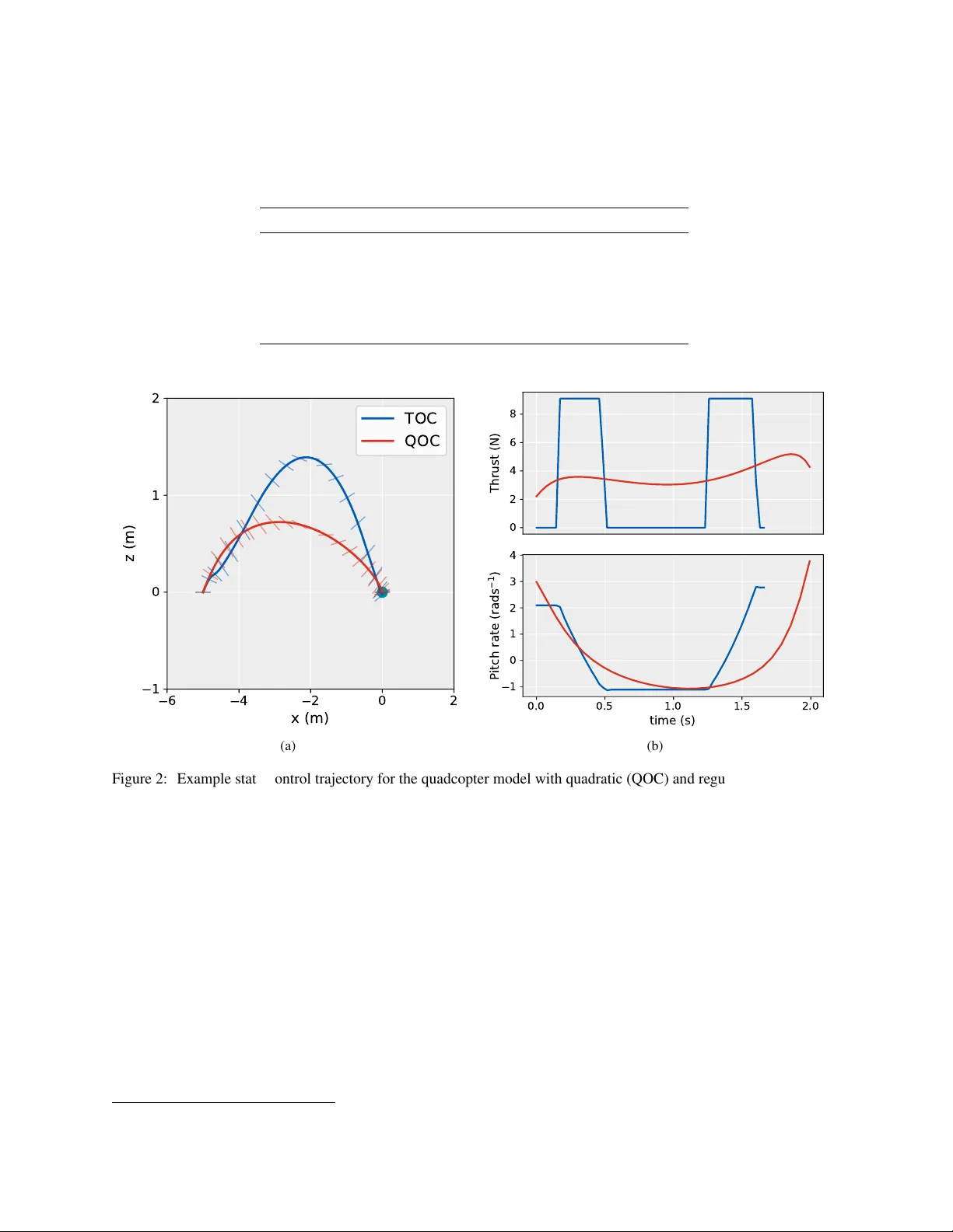
L E A R N I N G T H E O P T I M A L S T A T E - F E E D B A C K V I A S U P E RV I S E D I M I T A T I O N L E A R N I N G Dharmesh T ailor , Dario Izzo ∗ Advanced Concepts T eam European Space Agency Noordwijk, 2201 AZ Netherlands dharmesh.tailor@live.co.uk dario.izzo@esa.int A B S T R AC T Imitation learning is a control design paradigm that seeks to learn a control policy reproducing demonstrations from e xpert agents. By substit uting expert demonstrations for optimal behaviours, the same paradigm leads to the design of control policies closely approximating the optimal state- feedback. This approach requires training a machine learning algorithm (in our case deep neural networks) directly on state-control pairs originating from optimal trajectories. W e hav e shown in pre vious work that, when restricted to low-dimensional state and control spaces, this approach is very successful in se veral deterministic, non-linear problems in continuous-time. In this work, we refine our previous studies using as a test case a simple quadcopter model with quadratic and time-optimal objectiv e functions. W e describe in detail the best learning pipeline we hav e developed, that is able to approximate via deep neural netw orks the state-feedback map to a very high accurac y . W e introduce the use of the softplus acti vation function in the hidden units of neural netw orks showing that it results in a smoother control profile whilst retaining the benefits of rectifiers. W e sho w how to ev aluate the optimality of the trained state-feedback, and find that already with two layers the objectiv e function reached and its optimal value dif fer by less than one percent. W e later consider also an additional metric linked to the system asymptotic beha viour - time taken to con verge to the policy’ s fixed point. W ith respect to these metrics, we show that improv ements in the mean absolute error do not necessarily correspond to better policies. K eywords Optimal control · Deep learning · Imitation learning · G&CNET 1 Introduction The dynamic programming approach to deterministic optimal control indicates the existence of an optimal state-feedback map or policy [ 15 ]. This is a consequence of the Hamilton-Jacobi-Bellman (HJB) equation in continuous-time settings. If the solution is pursued in the viscosity sense [ 1 ] then such a solution is also unique, making the optimal control problem (in terms of the value function) well-posed in the Hadamard sense [ 9 ]. Howe ver , for most problems of interest analytic solutions to the HJB equation cannot be found and approximate methods are resorted to (e.g. [ 2 ]). This is particularly the case for systems modelled by non-linear dynamics or where the cost function is not quadratic in the state and control. The alternate approach to optimal control is Pontryagin’ s minimum principle [ 22 ] in which the optimal solution sought is one defined between two states (or sets) only (i.e. a single trajectory). When applicable, one can use the solutions coming from the repeated use of Pontryagin’ s principle to learn an approximation to the solution of the HJB equations [ 25 ]. This could be vie wed as a form of imitation learning (see [ 21 ] for an e xample of early pioneering work) defined as "[training] a classifier or r egr essor to replicate an e xpert’ s policy given training data of the encounter ed observations and actions performed by the expert" [ 23 ]. In our case the encountered observations and actions are substituted for ∗ Dario Izzo is the corresponding author optimal trajectories. In general, learning a policy from optimal control actions is a troublesome approach as reported in [ 19 ]. This has been attrib uted to the fact that the distrib ution of states the policy encounters during e xecution dif fers from the distribution the policy is trained on [ 24 ]. T o ov ercome the issue, various methods are proposed e.g. D A GGER [ 24 ]. These methods share in common the ability for the polic y being learned to influence the trajectories (and therefore states) contained within the training dataset. This is achiev ed by iterating between trajectory optimisation and polic y ex ecution whereby the states encountered constrain the optimal trajectories. In more recent years, the use of a trajectory optimiser to aid polic y learning has been in vestigated within reinforcement learning e.g. [ 17 , 18 ] with great success. It was reported that even D A GGER-like approaches are unsuccessful at tasks in volving contact dynamics or with high-dimensional state/action spaces. Instead it was proposed to augment the objectiv e function of the trajectory optimiser with a term measuring the de viation of the controls from the current polic y . Such work w as intended to fix the issues that arise when learning a policy from a database of optimal trajectories. Sánchez-Sánchez, et al. (2018) [ 25 ] demonstrated that when applied to low-dimensional problems and, in particular , systems that con ver ge to a small region of the state space, such issues do not arise and a straightforward approach is therefore desirable and v ery successful. This is attrib uted to the scaling up of the number of trajectories used resulting in a dense co verage of the state space for relativ ely low dimensional problems. Intuitiv ely this can be understood by considering a non-parametric policy in which control selection is based on a nearest-neighbour look-up in the library of trajectories [28]. Effecti ve learning from such large datasets was achiev ed using deep neural networks trained by stochastic gradient descent. It is worth noting here that feedforward networks were used despite training for a task resembling sequence prediction. This choice is justified by the Bellman optimality principle and can also be seen by considering that the solution to the HJB equation depends solely with respect to the current state. Despite this, neural networks with a recurrent architecture have been used in a similar context, for example in [ 6 ]), and could be advantageous when modelling errors or imperfect sensing are considered during simulation. In this work we b uild upon the work of Sánchez-Sánchez, et al. (2018) [ 25 ] using as a test case the tw o-dimensional quadcopter model with quadratic and time-optimal objecti ve functions considered there. This model was chosen due to its simplicity , to av oid this work becoming too in volved in the intricacies of a particular control problem. The generality of the methods presented means the insights drawn are equally applicable to other control problems pre viously considered such as spacecraft pinpoint landing [ 25 ] and orbital transfers [ 13 ]. W e describe in detail an improved learning pipeline and confirm that it is able to approximate the state-feedback map to a very high accuracy . In order to determine the limits on this accuracy , we perform a wider search on the hyperparameters of the neural networks, with particular attention to the depth and number of units per hidden layer . W e introduce the use of the softplus activ ation function in the hidden units sho wing how this results in a smoother and more meaningful control profile whilst retaining the benefits of rectifiers during training (e.g. improved gradient propagation in multi-layer networks). W e propose a new method to e valuate the optimality of the trained state-feedback, a voiding the comple xities that were introduced in [ 25 ], and find that already with two layers the objecti ve function reached and its optimal v alue diff er by less than one percent. W ith respect to this metric, we find that improv ements in the mean absolute error do not necessarily correspond to improv ed policies. For many of the trained policies, we observe that the resulting system stabilises at a nearby equilibrium state after reaching the tar get state. This property forms the basis of a second metric we consider and that describes the asymptotic behaviour of the system, namely the time tak en to con verge to the stability point. 2 Quadcopter model W e consider a two-dimensional model of a quadcopter with 3 de grees of freedom [ 11 ] in which the task is to manoeuvre the vehicle to a goal location (see Fig. 1). The system states x ∈ I R n x and control inputs u ∈ I R n u ( n x = 5 , n u = 2 ) are defined to be: x = [ x, v x , z, v z , θ ] T , u = [ F T , ω ] T (1) where x is the horizontal position, z is the vertical position, ( v x , v z ) is the velocity , θ is the pitch angle, F T is the total thrust force and ω is the pitch rate. The dynamics of the system is giv en by: ˙ x =      ˙ x ˙ v x ˙ z ˙ v z ˙ θ      = f ( x , u ) =      v x F T m sin θ − β v x v z F T m cos θ − g − β v z ω      (2) where g is the gravitational acceleration and m is the mass of the quadcopter . Compared with previous work [ 25 ], the dynamics hav e been modified to take into account the ef fect of drag forces via a drag coefficient β . The control inputs 2 x z ω F T θ Figure 1: T wo-dimensional model of a quadcopter considered in this study . Control inputs { F T , ω } as well as the state variables { x, z , θ } are indicated. are constrained as follows: 0 ≤ F T ≤ F max T , | ω | ≤ ω max (3) where F max T and ω max are limits on the maximum allow able thrust and pitch rate respectiv ely . As per the standard formulation of the optimal control problem, the task of manoeuvring the quadcopter is equiv alent to finding the state-control trajectory { x ( t ) , u ( t ) : 0 ≤ t ≤ T } satisfying: minimize u ( t ) , T J ( x ( t ) , u ( t ) , T ) sub ject to ˙ x ( t ) = f ( x ( t ) , u ( t )) ∀ t, x (0) = x o , x ( T ) = x f (4) where x o is the initial state, x f is the target state, J is the objectiv e function determining the path cost and T is the total trajectory time. W e consider two objecti ve functions, the first is quadratic control, J = Z T 0 || u ( t ) || 2 d t = Z T 0 ( F T ( t ) 2 + ω ( t ) 2 ) d t, (5) and the second seeks to minimise time, J = T . (6) There are multiple ways of solving optimal control problems of this form [ 4 ]. W e use a direct transcription and collocation method, namely Hermite-Simpson transcription, which transforms the trajectory optimisation problem into a non-linear programming (NLP) problem [ 5 ]. The modelling language AMPL was used to specify the NLP problem. This is then solved using an NLP solver , many of which are supported by AMPL. For our problem we used SNOPT [ 7 ], a sequental quadratic programming NLP solver . W e observe that this solver is able to con verge to the optimal solution starting from an arbitrary initial guess for most choices of the initial and target state. When solving the time optimal control problem, the resulting trajectories raised a few issues. The first was the occurrence of chattering in the control profiles. The second w as the very aggressiv e nature of the time optimal manoeuvres including mid-flight flips, which we wanted to avoid as the y limit the use of our results on real quadcopters where such manoeuvres would be considered unnecessarily dangerous. By penalising the time objectiv e with a weighted cost functional quadratic in ω , we were able to eliminate chattering in the profiles of both control inputs. The weighting factor α was tuned such that chattering was removed across a range of choices for the initial and final state. The regularised time objecti ve function is: J = T + α Z T 0 ω ( t ) 2 d t, where α = 0 . 1 (7) Clearly this has the effect of making the resulting solutions sub-optimal with respect to the original objecti ve function. The v alue of α was thus chosen such that the optimal time w as only marginally increased. Con vergence in the time- optimal case was also improved using the follo wing continuation procedure: we first solve for the original problem and then use the solution as an initial guess for the re gularised problem. Preventing flips means keeping the orientation of 3 the quadcopter close to upright. This was achie ved by adding the follo wing path constraint: | θ | ≤ θ max . An example trajectory for both objecti ve functions is sho wn in Fig. 2. A summary of all numerical parameters and their values 2 is stated in T able 1. T able 1: Numerical parameters of the quadcopter model Parameter V alue Description m 0 . 38905 kg Mass of the quadcopter g 9 . 81 m s − 1 Acceleration due to Earth’ s gravity β 0 . 5 Drag coefficient θ max π / 4 rad Maximum pitch angle F max T 9 . 1 N Maximum thrust ω max 35 rad s − 1 Maximum pitch rate 6 4 2 0 2 x (m) 1 0 1 2 z (m) TOC QOC (a) 0 2 4 6 8 T h r u s t ( N ) 0.0 0.5 1.0 1.5 2.0 time (s) 1 0 1 2 3 4 P i t c h r a t e ( r a d s 1 ) (b) Figure 2: Example state-control trajectory for the quadcopter model with quadratic (QOC) and regularised time (TOC) objectiv e functions. For the presented example, the initial state is ( x = − 5 , z = 0 , v x = 2 , v z = 2 , θ = 0 ) and the target state is 0 (green dot). (a) State trajectory plotted for the position v ariables ( x, z ) with the pitch angle indicated. (b) Corresponding optimal control profiles. W e note that with respect to the thrust profile (top right), QOC is continuous and TOC is bang-bang. 3 State-feedback approximation For each control task (either quadratic or time objectiv e functions), we seek to learn a close approximation to the optimal state-feedback map that na vigates the quadcopter from arbitrary initial states, within a specified region of the state space, to some fixed target state. Optimal trajectories are generated using the method described in 2. These can be considered demonstrations of the optimal policy π ∗ from which a regressor is trained to approximate the mapping from state to optimal control. W e first define our state space as the compact set X ⊂ I R n x where closed interv als are specified for each dimension (see T able 2). This constrains the optimal trajectories to belong to this region. The intervals ha ve changed with respect to our previous w ork [ 25 ]. Since we consider the problem of quadcopter manoeuvres rather than landing, the interv als now contain the tar get state and the endpoints are equidistant from the target. Then M states are drawn uniformly , x ( i ) o ∼ U ( X ) for i = 1 , ..., M , each corresponding to an initial state of a trajectory optimisation 2 V alues used are based on the Parrot Bebop drone 4 problem to be solved (the final state is k ept constant). M must be chosen suitably large as to ensure a dense co verage of the state space. T able 2: State space intervals State variable Interv al x [ − 10 , 10] m z [ − 10 , 10] m v x [ − 5 , 5] m s − 1 v z [ − 5 , 5] m s − 1 θ [ − π 4 , π 4 ] rad For each trajectory optimisation problem, the solv er outputs a sequence of state-control pairs of the form: τ i = ( x ( i ) j , u ( i ) j ) J j =1 where x ( i ) 1 = x ( i ) o , x ( i ) J = x f i = 1 , ..., M (8) where J is the number of points on a uniformly spaced grid. The level of discretisation is determined by the number of nodes K chosen in the direct transcription method. Since the Hermite-Simpson transcription method was used, the midpoints of the nodes are also e valuated thus the number of grid points J is 2 K − 1 . A summary of the parameters used for the large-scale trajectory generation and the values chosen is provided in T able 3; this is the same for both objectiv e functions. As stated in Section 2, the optimal trajectory could be found with the solver simply presented with an arbitrary initial guess for most initial conditions. This means each trajectory optimisation problem could be solved independently allo wing for parallelization of trajectory generation thus speeding up the process and resulting in a considerably lar ger dataset than previously considered. W e also note that an unintended benefit of this approach is the distribution of initial conditions has more uniform co verage of the state space. This is a consequence of directly sampling the initial conditions rather than the random walk approach adopted in [6]. For each control task, it took approximately 1 hour to generate the corresponding library of trajectories when distributed o ver 40 CPUs. T able 3: Dataset generation parameters Parameter V alue Description x f 0 Final state M 200 000 Number of trajectories K 30 Number of nodes W e then construct the datasets by con verting each library of trajectories into a collection of state-control pairs, { ( x i , u i ) } N i =1 with N = M · J , where trajectory information and ordering is discarded. Since the trajectories hav e the same final state, the distrib ution of inputs within the datasets is ske wed tow ards the target state. Despite this, we find that the lack of uniformity does not pose a problem when fitting a regressor to approximate the map from states to controls. Once trained, the regressor is a deterministic policy π : X → U where X is the state space defined previously and U is the compact set corresponding to the constraints in T able 1. 4 Deep neural network training W e approach this in the standard machine learning way . Firstly each dataset is partitioned into a training set (90%) and a held-out test set (10%) such that state-control pairs in each set come from distinct trajectories. The datasets are also preprocessed by way of scaling features of both the inputs and tar gets to have zero mean and unit v ariance. There are many machine learning algorithms appropriate for this task. W e choose to train neural networks as regressors. This is motiv ated by their high degree of flexibility (e.g. number of hidden layers, number of units per layer etc.) allo wing for a comparison based on the amount of parameterisation. Furthermore, giv en the size of the dataset generated, we can use specialised libraries for neural networks that can take advantage of GPUs for faster training. In our case, we perform neural network training in Keras ex ecuted on a NVIDIA GeForce GTX 1080 Ti GPU. W e restrict our attention to feedforward, fully-connected networks with equal number of units in the hidden layers and a squared error loss function. In contrast to previous work [ 25 ], we consider the problem of jointly learning both targets (controls) in a single regressor . It is worth noting that since the thrust control for time-optimal control has a bang-bang structure, the 5 learning problem for this particular target could be structured as a classification task. W e decided against pursuing this as we seek to demonstrate a policy learning pipeline applicable to the broadest set of control problems. From pre vious work, we take the best performing acti vation functions, that is the non-saturating rectified linear non- linearity (ReLU) [ 20 ], with analytic form f ( x ) = max(0 , x ) , for the hidden layers and hyperbolic tangent for the output layer . Since the hyperbolic tangent is bounded, the targets in the dataset are further scaled to lie within the range [-1,1]. W eights are initialised using Xavier’ s uniform method [ 8 ]. W e use the Adam optimiser , a v ariant of gradient descent optimisation, with its default v alues [ 14 ]. This was settled on after a comparison with plain stochastic gradient descent with momentum, a widely used non-adaptiv e optimiser . The minibatch size was fix ed to 512; this was chosen after a number of preliminary trials. W e found that reducing the minibatch size to v ery small values consistently resulted in a substantial drop in the performance. This is in contrast to accepted deep learning practice that smaller minibatch sizes result in better generalisation [ 16 ]. W e partition each training set gi ving a validation set (10% held out) that is used to track performance during training. This is necessary for early stopping for which training ends if no improv ement in the validation loss is observ ed for more than 5 epochs. The state of the network is sa ved after e very epoch and the final parameter v alues selected at the end of a training run are those that gav e the smallest validation loss. W e also use a learning rate schedule in which the learning rate drops by a factor of 2 if there is no improv ement in the validation loss for 3 epochs. 1 0 6 1 0 5 1 0 4 1 0 3 1 0 2 learning rate loss 1 0 5 1 0 4 1 0 3 1 0 2 learning rate d loss Figure 3: Learning rate finder method from [ 26 ]. Learning rate is increased on a logarithmic scale during training of a single epoch starting from a small value. Optimal learning rate is the one that giv es the largest decrease in the loss. Left : Initially with small learning rates, the loss improves slowly . As the learning rate increases, the loss improves faster until it explodes (not shown) when the learning rate becomes very large. Fastest decrease in the loss is when the slope of the loss curve is the most negati ve (dotted red line). Right : Plot of the change in loss per iteration with a moving a verage filter applied. The optimal learning rate is the minimum of this curve (dotted red line). Despite using an adaptiv e optimiser , the initial learning rate still needs to be appropriately set. The learning rate is one of the most important hyperparameters and the success of a gi ven training run is lar gely determined by it [ 3 ]. Giv en that we plan to experiment with many netw ork architectures, performing a grid (or better random) search on the learning rate would be too time consuming. W e instead use a simple b ut relativ ely unknown method from [ 26 ] to determine a suitable initial learning rate. This works by training for a single epoch, with the learning rate initially set to a very small value (e.g. 10 − 6 ), whilst increasing the learning rate at each iteration (i.e. minibatch update). The particular v alue of the learning rate that giv es rise to the largest decrease in the loss is the optimal learning rate (ignoring stochasticity due to the order and batching of the training examples) - see Fig. 3. Since the learning rate is decayed during training, we round the optimal rate up to the nearest po wer of 10 and set this to be the initial learning rate in the full training run. For the majority of networks, the initial learning rate was set to 10 − 3 ; only for the deeper and wider architectures did the method indicate a smaller initial learning rate of 10 − 4 . 5 T raining experiments W e train a large number of networks with dif ferent architectures all following the same training procedure described in Section 4. W e consider networks with the hyperparameters: no. of units per hidden layer: {50,100,200,500,1000}; no. of layers: [1..10]. The purpose of this is to in vestigate limits on the maximum attainable performance of the datasets. W e ev aluate the networks using the mean absolute error (MAE) metric, shown in T able 4, and from now on ‘error’ should be read as meaning MAE. 6 T able 4: Mean absolute error on the test set ev aluated for each dataset: Quadratic optimal control (QOC) and T ime optimal control (TOC). Neural networks are compared by their architecture where “units” and “layers” in the 1st column heading refer to the number of units per hidden layer and the number of hidden layers respecti vely . The “normalised” column gi ves the error on the dataset after preprocessing and a veraged for both targets. The columns “ u 1 ” and “ u 2 ” gi ve the error on the datasets before preprocessing ev aluated for each target separately . For each number of units considered, the network architecture with the best performance is highlighted for both datasets. Network architecture - QOC error TOC error normalised u 1 u 2 normalised u 1 u 2 50-1 0.0293 0.2132 0.3931 0.0506 0.3737 0.3957 50-2 0.0127 0.0903 0.1839 0.0282 0.2096 0.2120 50-3 0.0094 0.0667 0.1364 0.0224 0.1711 0.1480 50-4 0.0096 0.0683 0.1394 0.0203 0.1509 0.1541 50-5 0.0077 0.0554 0.1055 0.0197 0.1463 0.1509 50-6 0.0075 0.0543 0.1008 0.0187 0.1377 0.1464 50-7 0.0073 0.0531 0.0995 0.0188 0.1382 0.1476 50-8 0.0072 0.0527 0.0978 0.0186 0.1368 0.1474 50-9 0.0072 0.0526 0.0966 0.0186 0.1372 0.1438 50-10 QOC,TOC 0.0072 0.0523 0.0968 0.0185 0.1372 0.1422 100-1 0.0223 0.1586 0.3260 0.0455 0.3342 0.3606 100-2 0.0087 0.0635 0.1141 0.0252 0.1963 0.1498 100-3 0.0070 0.0516 0.0909 0.0185 0.1439 0.1105 100-4 0.0067 0.0496 0.0858 0.0181 0.1379 0.1197 100-5 0.0066 0.0487 0.0835 0.0175 0.1337 0.1162 100-6 0.0066 0.0487 0.0821 0.0175 0.1334 0.1172 100-7 0.0066 0.0485 0.0818 0.0174 0.1325 0.1152 100-8 0.0065 0.0482 0.0817 0.0174 0.1322 0.1184 100-9 TOC 0.0065 0.0481 0.0825 0.0174 0.1320 0.1174 100-10 QOC 0.0065 0.0481 0.0818 0.0174 0.1326 0.1171 200-1 0.0176 0.1276 0.2385 0.0406 0.3043 0.2952 200-2 0.0077 0.0569 0.0961 0.0220 0.1775 0.1040 200-3 0.0064 0.0475 0.0778 0.0175 0.1377 0.0980 200-4 0.0081 0.0597 0.1021 0.0169 0.1318 0.1007 200-5 0.0063 0.0467 0.0761 0.0168 0.1297 0.1055 200-6 TOC 0.0062 0.0462 0.0754 0.0166 0.1292 0.0976 200-7 0.0062 0.0459 0.0744 0.0166 0.1290 0.1018 200-8 0.0062 0.0461 0.0749 0.0167 0.1294 0.1008 200-9 0.0062 0.0460 0.0745 0.0169 0.1312 0.1043 200-10 QOC 0.0061 0.0458 0.0742 0.0167 0.1298 0.1021 500-1 0.0137 0.1004 0.1759 0.0353 0.2749 0.2119 500-2 0.0065 0.0488 0.0793 0.0195 0.1563 0.0952 500-3 0.0062 0.0462 0.0745 0.0169 0.1340 0.0908 500-4 0.0061 0.0456 0.0734 0.0165 0.1295 0.0945 500-5 TOC 0.0060 0.0451 0.0724 0.0161 0.1268 0.0889 500-6 0.0067 0.0492 0.0866 0.0163 0.1283 0.0906 500-7 0.0060 0.0447 0.0713 0.0172 0.1333 0.1063 500-8 0.0059 0.0444 0.0691 0.0163 0.1276 0.0942 500-9 0.0059 0.0443 0.0692 0.0220 0.1653 0.1582 500-10 QOC 0.0059 0.0442 0.0692 0.0164 0.1285 0.0945 1000-1 0.0142 0.1058 0.1722 0.0310 0.2478 0.1546 1000-2 0.0064 0.0476 0.0759 0.0185 0.1485 0.0916 1000-3 0.0061 0.0455 0.0720 0.0166 0.1311 0.0888 1000-4 0.0060 0.0448 0.0709 0.0160 0.1267 0.0864 1000-5 0.0059 0.0443 0.0696 0.0161 0.1274 0.0863 1000-6 TOC 0.0059 0.0441 0.0689 0.0160 0.1269 0.0853 1000-7 0.0058 0.0438 0.0679 0.0161 0.1271 0.0872 1000-8 0.0058 0.0439 0.0682 0.0161 0.1266 0.0904 1000-9 QOC 0.0058 0.0435 0.0672 0.0162 0.1268 0.0916 1000-10 0.0058 0.0439 0.0680 0.0196 0.1495 0.1303 7 0 10 20 30 40 50 60 70 number of epochs 0.0026 0.0027 0.0028 0.0029 0.0030 0.0031 loss train valid Figure 4 : T raining and validation set loss, as a function of the number of training epochs, for the neural network with 1000 units per hidden layer and 10 hidden layers e valuated on the quadratic optimal control dataset. W e should note that the errors are not definiti ve for each architecture. This is because we did not repeat training with different random seeds and the other hyperparameters (e.g. minibatch size) were not fine-tuned. Despite this, the random seed for each network was initialised independently and so the results are demonstrativ e of how changes in the network architecture af fect performance. Consistent with pre vious work [ 25 ], when comparing the normalised errors between the two datasets, we observ e the error for quadratic optimal control (QOC) to be consistently smaller than that of time optimal control (TOC). This is not surprisingly as the controls (particularly the thrust) is continuous with saturated re gions for QOC and bang-bang for TOC. For a gi ven number of units, we observe that, as the number of layers increases, the error initially decreases as expected. Howe ver , after approximately 5 hidden layers, there is little further improvement - the error saturates or in a fe w cases increases. W e also observ e a difference in beha viour here between the datasets, that is for QOC, the best architecture consistently appears to be the one with 10 layers albeit only small improvement compared with 5 layers or more. Howe ver , for TOC, we observe that with 200 units or more, the best performing network is the one with 5 or 6 hidden layers. In all, this suggests that stacking more layers is ineffecti ve after a certain point and an increase in the number of units is necessary to gain an improv ement in performance. By looking at the final values of the training and v alidation loss across all networks, we observe that overfitting is v ery minor . For instance the highest parameterised network trained on QOC ov erfit by under 2%. This learning curve is shown in Fig. 4. W e can see that from approximately 30 epochs the training loss plateaus. Despite training continuing for 40 more epochs, the increase in the v alidation loss is not considerable. This indicates that we are still operating in an underfitting regime suggesting further improvement is possible. It is likely the reason for the underfitting is the large training set size. Considering the highest parameterised network, this has fewer parameters than the number of training set datapoints (9,017,002 vs 9,440,000). Thus, the training set size had a re gularising effect eliminating the need for techniques such as DropOut [27] or weight decay . W e found that adding more layers led to a higher training loss. This degr adation problem is a common occurrence in deep learning. Methods have been de veloped in recent years to alle viate this such as batch normalisation [ 12 ] and residual connections [ 10 ]. W e decided against pursuing this due to the saturation observed with the depths already considered. Although it is likely we would ha ve been able to further reduce the error with more units per layer , we also observed saturation in the test error - see the shaded ro ws in T able 4. 6 Policy ev aluation For a given dataset, the different neural networks correspond to different instances of the same control policy . As shown in T able 4, the neural networks v ary in their accuracy at reproducing the state-to-control mapping of the optimal trajectories. Even the highest parameterised neural network does not reproduce the mapping exactly exhibiting a minimum error . Therefore, the resulting policies can only be considered to be approximations to the optimal state- feedback. Despite this, the difference between prediction and ground truth is small when compared to the range of control values that can be attained. 8 The policies must also be ev aluated on their ability to perform the control task. By numerical integration of the system dynamics with the policy substituted for the control inputs we can compute the state trajectory , x ( t ) = x o + Z t 0 f ( x ( τ ) , π ( x ( τ ))) d τ , (9) starting from any initial state x (0) = x o . This can be seen as a closed-loop (feedback) control strategy . Clearly , the control trajectory can also be computed by ev aluating the policy at predefined intervals along the state trajectory . W e repeat the analysis undertaken in [ 25 ] and find that all the policies (including the lowest parameterised neural networks) e ventually reach the target state with small error . This is the case regardless of the initial state, provided it is contained within the state space. Also the resulting trajectories closely resemble the optimal trajectory for the equi valent manoeuvre. After the target state is reached, the system stabilises at a state close to the tar get in terms of x and z . The v x , v z and θ components must be zero. This hovering phase, reported in [ 25 ], is achiev ed when the thrust predicted by the neural network cancels m · g and the pitch rate takes a value close to 0 , as determined by the quadcopter dynamics. W e now further inv estigate the trained policies by looking at the performance up to when it reaches the target (the manoeuvr e phase) and the behaviour during the ho vering phase. 6.1 T rajectory optimality W e shall in vestigate whether there is any relationship between the accuracy of a polic y’ s state-feedback approximation and its performance on the control task. For this we look at relati ve optimality , one of the e valuation metrics used in previous w ork [ 25 ]. This in volves e valuating the objecti ve function J on a state-control trajectory resulting from some policy and then computing the relativ e error of this value with respect to that of the optimal trajectory . This is then repeated for multiple manoeuvres giving an a verage relativ e optimality . W e have improved the algorithm for determining relativ e optimality . Previously , a fixed integration time was used regardless of distance from the tar get state. The trajectory was then truncated such that the final state is the one closest to the target. This raised a few issues. The first is that, in the distance metric, the state v ariables were scaled to ov ercome the problem of unit heterogeneity . This made the trajectory time sensitiv e to the choice of scale factors. More concerning was that if the system stabilises near the target then the closest state might be reached during the ho vering phase. This could ske w the results as the objecti ve value of the optimal trajectory is restricted to the manoeuvre. T o ov ercome these issues, we use, for the integration time, the final time of the corresponding optimal trajectory . Full details are outlined in algorithm 1. Algorithm 1 Policy trajectory optimality 1: Given initial state x o and final time t f of trajectory from test set 2: Compute trajectory arising from policy with initial state x o and integration time t f 3: Extract final state x f from policy trajectory 4: Solve for optimal trajectory with initial state x o and final state x f 5: Evaluate objecti ve function on policy trajectory and optimal trajectory: j π , j ∗ 6: Compute relative error: ( j π − j ∗ ) /j ∗ In general, we observe that all the policies, e ven those represented by shallo w neural networks, are close-to-optimal. Furthermore, the quadratic-optimal policies have a smaller relativ e optimality error than the time-optimal policies. This is consistent with the state-feedback approximation performance between the two datasets observed pre viously . The error between the optimal cost and the policy cost appears to initially reduce as the corresponding policy’ s state- feedback approximation error decreases (see T able 5). Howe ver , the relationship does not continue for neural networks with greater depths despite their state-feedback approximation error continuing to decrease. W e should emphasise that the improv ement in state-feedback approximation is not very considerable after a netw ork depth of 3. The results indicate that despite similar state-feedback approximations, when such errors are propagated during integration of the system, they result in v arying values of the trajectory cost. This sho ws that finding the regressor with the lo west state-feedback approximation error is not necessary as small improv ements are not reflected in the policy optimality . W e should highlight that the errors are rather small, with the time optimal case resulting in a time loss of a few milliseconds at most in the best networks. This confirms the extreme precision achiev able by the pursued approach, at least on the low dimensional dynamics here considered. 9 T able 5: Relativ e error of each objectiv e function, quadratic optimal control (QOC) and time optimal control (T OC), ev aluated on the policy trajectory with respect to the objective v alue of the optimal trajectory av eraged over trajectories from the test set. This is shown for policies represented by neural networks with 100 units per hidden layer accompanied by the corresponding test set error . Network architecture - QOC TOC MAE Optimality (%) MAE Optimality (%) 100-1 0.0223 1.674 0.0455 2.475 100-2 0.0087 0.266 0.0252 0.900 100-3 0.0070 0.199 0.0185 0.605 100-4 0.0067 0.206 0.0181 0.793 100-5 0.0066 0.238 0.0175 0.664 100-6 0.0066 0.241 0.0175 0.759 100-7 0.0066 0.299 0.0174 0.648 100-8 0.0065 0.220 0.0174 0.707 100-9 0.0065 0.239 0.0174 0.740 100-10 0.0065 0.207 0.0174 0.669 6.2 Asymptotic behaviour W e find that the system stabilises to the same point regardless of the initial state. The equilibrium point x e for each policy is defined by f ( x e , π ( x e )) = 0 . A consequence of the dataset generation process is that the target state is by far the majority state in the datasets. Howe ver , the corresponding control for this state across instances is not identical. This is a consequence of the optimal control solver used which, for the control at the target state, simply giv es a smooth continuation of the preceding controls in the trajectory . In fact, the change in the intervals, particularly the z dimension, from which the initial states of the optimal trajectories were sampled from resulted in a shift in the distrib ution of control v alues at x f . Although this was not the intention of the change, for both datasets the mean of this distribution turned out to be closer to [ mg , 0] . W e noticed consistently that the system now stabilised much closer to the target than before. This suggests that the distance of the equilibrium point from the target is related to the controls predicted by the policy at x f . This allows for the possibility of the equilibrium point being influenced at training time. W e determine the equilibrium point for sev eral neural networks and find that, for both control tasks, the network whose policy’ s equilibrium point is furthest from the tar get is the one with the lo west accuracy in state-feedback approximation (see ‘100-1’ in T able 6). A consequence of the quadcopter dynamics is that x e for all policies is non-zero only in the x and z dimensions and we consider a target state that is zero in all variables. Since the units are equiv alent, any distance metric would be suitable here and hence we use Euclidean distance. By considering the definition of stability , for dif ferent radii we ev aluate the time at which the system first enters into a ball centred at its equilibrium point. This time is av eraged ov er many different trajectories starting from initial states taken from the test set, giving a stability time for each policy and ball radius (T able 6). T o av oid aggregating values with different units, we use the Chebyshe v distance as the metric to define the ball. This constrains all state variables to lie a giv en distance from x e . Given an equilibrium point x e and radius r , we define the ball as: B r ( x e ) = { x ∈ I R n x | max i ( | x i − ( x e ) i | ) < r } . As expected, we observ e the stability time to increase as the ball radius decreases. W e also observ e the stability time for the time-optimal policies to be lo wer for the largest ball radius considered. For the larger radii, the stability times are similar . Furthermore, we observe the stability time to be greater for policies where x e is further from x f . This is clear when comparing the network architecture ‘100-1’ against the others in T able 6. 7 Softplus units W e ha ve sho wn that neural networks can reproduce the state-to-control mapping of optimal trajectories with low error and that the cost of the policy trajectories is v ery close to the optimal cost. For quadratic optimal control, we observ e the optimal trajectories to hav e a control profile that is smooth. Although having little ef fect on the state trajectory , the control profile of the polic y trajectories exhibit sharp changes in direction. W e should emphasise that the dif ference here is often indistinguishable, particularly for networks with more than one hidden layer . The neural networks we ha ve been training thus far are composed of piecewise linear functions (ReLUs). W e hypothesise that the current deficiency is the 10 T able 6: A verage time taken for policies to stabilise at their equilibrium point. This is shown for dif ferent radii r and network architectures for both control tasks: quadratic optimal control (QOC) and time optimal control (TOC). Network architecture - Distance of equilibrium from target Stability time (s) r = 10 − 1 r = 10 − 2 r = 10 − 3 r = 10 − 4 r = 10 − 5 QOC 100-1 0.0118 2.728 5.228 8.910 13.102 17.200 100-2 0.0023 2.455 2.513 3.592 5.089 6.486 100-3 0.0025 2.453 2.509 3.094 3.634 4.421 100-4 0.0057 2.453 2.540 3.561 4.502 6.034 100-5 0.0025 2.452 2.518 3.090 3.779 4.481 TOC 100-1 0.1058 3.021 6.003 9.252 12.454 15.398 100-2 0.0302 1.987 5.052 8.316 10.876 13.370 100-3 0.0138 1.957 2.340 2.905 3.447 3.991 100-4 0.0180 1.963 2.426 3.317 4.104 4.920 100-5 0.0192 1.958 2.530 3.290 4.035 4.788 result of attempting to approximate a smooth function (i.e. the optimal state-feedback for QOC) with a non-smooth function. W e in vestigate the ef fect of training neural networks that, for the intermediate units, use a smooth version of ReLU called softplus for the activ ation function. This has the analytic form: f ( x ) = log(1 + exp( x )) . This keeps useful properties of ReLU such as its unboundedness, necessary for ov ercoming the v anishing gradient problem. The performance of such networks trained using the same procedure as in Section 4 is comparable to those trained previously (see T able 7). For quadratic optimal control, except for netw orks with a single hidden layer , we consistently find lower error in the softplus networks. W e can also confirm that the relativ e optimality of the resulting policies is similar to those reported previously . In Fig. 5, for two policies corresponding to a ReLU and softplus network, we sho w ho w the thrust and pitch rate change when z and x are v aried respectively about 0 with the other state v ariables fixed at the origin. W e observ e that, whilst the policies with ReLU and softplus netw orks behav e similarly , the controls for the softplus netw ork have the desireable property of a smooth curve. 1.0 0.5 0.0 0.5 1.0 V e r t i c a l p o s i t i o n ( m ) 0 2 4 6 8 T h r u s t ( N ) m g softplus relu 1.0 0.5 0.0 0.5 1.0 H o r i z o n t a l p o s i t i o n ( m ) 4 2 0 2 4 6 P i t c h r a t e ( r a d s 1 ) Figure 5: Comparison of the control profiles of policies derived from ReLU and softplus neural networks for quadratic optimal control. The controls necessary for the system to be at equilibrium are indicated (grey dashed line). 11 T able 7: Comparison of test set performance between ReLU and softplus neural networks. The metric shown corresponds to the ‘normalised’ error . W e highlight networks with the lowest error . Network architecture - QOC error TOC error ReLU softplus ReLU softplus 50-1 0.0293 0.0317 0.0506 0.0558 50-2 0.0127 0.0113 0.0282 0.0302 50-3 0.0094 0.0079 0.0224 0.0281 50-4 0.0096 0.0075 0.0203 0.0218 50-5 0.0077 0.0079 0.0197 0.0200 50-6 0.0075 0.0065 0.0187 0.0184 50-7 0.0073 0.0063 0.0188 0.0184 50-8 0.0072 0.0066 0.0186 0.0180 50-9 0.0072 0.0074 0.0186 0.0182 50-10 0.0072 0.0093 0.0185 0.0180 100-1 0.0223 0.0303 0.0455 0.0536 100-2 0.0087 0.0084 0.0252 0.0285 100-3 0.0070 0.0072 0.0185 0.0219 100-4 0.0067 0.0061 0.0181 0.0193 100-5 0.0066 0.0061 0.0175 0.0177 100-6 0.0066 0.0064 0.0175 0.0174 100-7 0.0066 0.0059 0.0174 0.0174 100-8 0.0065 0.0060 0.0174 0.0170 100-9 0.0065 0.0060 0.0174 0.0170 100-10 0.0065 0.0061 0.0174 0.0168 200-1 0.0176 0.0282 0.0406 0.0437 200-2 0.0077 0.0073 0.0220 0.0262 200-3 0.0064 0.0066 0.0175 0.0206 200-4 0.0081 0.0059 0.0169 0.0180 200-5 0.0063 0.0059 0.0168 0.0174 200-6 0.0062 0.0059 0.0166 0.0168 200-7 0.0062 0.0059 0.0166 0.0168 200-8 0.0062 0.0062 0.0167 0.0172 200-9 0.0062 0.0059 0.0169 0.0169 200-10 0.0061 0.0061 0.0167 0.0240 8 Discussion and future work W e show that the straightforward approach of constructing a near-optimal control policy by supervised learning on trajectories satisfying Pontryagin’ s principle of optimality is successful in the lo w-dimensional problem here considered. In addition to the lo w error achiev ed in the state-feedback approximation of the trajectories, for a majority of the trained policies, their optimality , from aggregating the cost from dif ferent initial states, is just up to a percent worse than that of the optimal. Furthermore, the policies exhibit various desirable properties such as consistent state con vergence regardless of initial condition. W e performed lar ge-scale training of man y neural network architectures on t wo datasets corresponding to quadratic- optimal and time-optimal trajectories for a simple quadcopter model in two-dimensions. In both cases, we were able to saturate the state-feedback approximation error after a certain amount of parameterisation. W e also conclude that the networks do not necessarily need to be very deep, finding 5 or 6 hidden layers to be adequate. For the time-optimal dataset, we found that incorporating ev en more layers was detrimental to the final performance. W e did not use any form of regularisation, in contrast to standard practice in deep learning, as we found that the use of large datasets meant that we were always operating in an underfitting re gime. W e only observ e a positive relationship between state-feedback approximation accurac y and policy optimality for the shallo wer networks. This can be understood as initially increasing the number of layers giv es rise to the largest increase in feedback approximation accurac y . Howe ver , we observe that small gains in the feedback approximation does not translate to better optimality . W e show that it is not necessary to find the best feedback approximation. It is possible to 12 identify a threshold after which the policy optimality is equi valent thereby constraining the hyperparameter search on the architecture. W e observe that the system, when controlled by the trained policies, stabilise at a state unique to each policy . This allowed us to consider an additional metric, that is the time taken to reach this con ver gent state. W e observe that this con ver gent state or equilibrium point appears to be further from the target state for policies with w orse state-feedback approximation accuracy . This also coincides with a longer time to reach the equilibrium point. The last in vestigation in volv ed changing the activ ation function of the units in the hidden layers to softplus, a smooth approximation to the rectifier . In addition to gi ving a similar state-feedback approximation accuracy , we observe the control profiles of the resulting policies to hav e a smooth behaviour (for quadratic-optimal control) - a property preferable for control systems. This suggests that best practices in deep learning, such as the use of rectifiers, are not always transferable to problems in continuous control. W e noted the regularisation ef fect that training on large datasets had on learning the optimal state-feedback. A further av enue of research would be to in vestigate ho w this effect v aries with different dataset sizes. From statistical learning theory , the difference between the final training and test set loss values gi ves an indication of overfitting. In vestigating how this v aries with different dataset sizes would help in understanding the sample comple xity of this method. In this work, we continued with the same low-dimensional dynamical model used in previous work [ 25 ]. The next logical step in this line of research would be inv estigating the effecti veness of this approach for higher dimensional systems. References [1] B A R D I , M . , A N D C A P U Z Z O - D O L C E T TA , I . Optimal control and viscosity solutions of Hamilton-Jacobi-Bellman equations. Birkhäuser (1997). [2] B E A R D , R . W. , S A R I D I S , G . N . , A N D W E N , J . T. Galerkin approximations of the generalized Hamilton-Jacobi- Bellman equation. A utomatica 33 , 12 (1997), 2159–2177. [3] B E N G I O , Y . Practical recommendations for gradient-based training of deep architectures. In Neural networks: T ricks of the trade . Springer , 2012, pp. 437–478. [4] B E T T S , J . T. Survey of numerical methods for trajectory optimization. Journal of guidance, control, and dynamics 21 , 2 (1998), 193–207. [5] B E T T S , J . T. Practical methods for optimal contr ol and estimation using nonlinear pr ogramming , v ol. 19. Siam, 2010. [6] F U R FA R O , R . , B L O I S E , I . , O R L A N D E L L I , M . , D I L I Z I A , P . , T O P P U T O , F . , L I N A R E S , R . , E T A L . A recurrent deep architecture for quasi-optimal feedback guidance in planetary landing. In IAA SciT ech F orum on Space Flight Mechanics and Space Structur es and Materials (2018), pp. 1–24. [7] G I L L , P . E . , M U R R A Y , W . , A N D S AU N D E R S , M . A . Snopt: An SQP algorithm for large-scale constrained optimization. SIAM r eview 47 , 1 (2005), 99–131. [8] G L O RO T , X . , A N D B E N G I O , Y . Understanding the difficulty of training deep feedforw ard neural networks. In Pr oceedings of the thirteenth international conference on artificial intelligence and statistics (2010), pp. 249–256. [9] H A D A M A R D , J . Sur les problèmes aux dérivées partielles et leur signification physique. Princeton university bulletin (1902), 49–52. [10] H E , K . , Z H A N G , X . , R E N , S . , A N D S U N , J . Deep residual learning for image recognition. In Pr oceedings of the IEEE confer ence on computer vision and pattern r ecognition (2016), pp. 770–778. [11] H E H N , M . , R I T Z , R . , A N D D ’ A N D R E A , R . Performance benchmarking of quadrotor systems using time-optimal control. A utonomous Robots 33 , 1-2 (2012), 69–88. [12] I O FF E , S . , A N D S Z E G E DY , C . Batch normalization: Accelerating deep network training by reducing internal cov ariate shift. In International Confer ence on Machine Learning (2015), pp. 448–456. [13] I Z Z O , D . , S P R A G U E , C . , A N D T A I L O R , D . Machine learning and evolutionary techniques in interplanetary trajectory design. arXiv pr eprint arXiv:1802.00180 (2018). [14] K I N G M A , D . P . , A N D B A , J . Adam: A method for stochastic optimization. arXiv pr eprint (2014). [15] K I R K , D . E . Optimal contr ol theory . Prentice-Hall, 1970. 13 [16] L E C U N , Y . A . , B OT T O U , L . , O R R , G . B . , A N D M Ü L L E R , K . - R . Efficient backprop. In Neural networks: T ricks of the trade . Springer , 2012, pp. 9–48. [17] L E V I N E , S . , A N D K O LT U N , V . Guided policy search. In International Confer ence on Machine Learning (2013), pp. 1–9. [18] L E V I N E , S . , A N D K O LT U N , V . V ariational policy search via trajectory optimization. In Advances in Neural Information Pr ocessing Systems (2013), pp. 207–215. [19] M O R DATC H , I . , A N D T O D O ROV , E . Combining the benefits of function approximation and trajectory optimization. In In Robotics: Science and Systems (RSS (2014), Citeseer . [20] N A I R , V . , A N D H I N T O N , G . E . Rectified linear units improve restricted boltzmann machines. In Pr oceedings of the 27th international confer ence on machine learning (ICML-10) (2010), pp. 807–814. [21] P O M E R L E AU , D . A . Alvinn: An autonomous land v ehicle in a neural network. In Advances in neural information pr ocessing systems (1989), pp. 305–313. [22] P O N T RY A G I N , L . S . , B O LT Y A N S K I I , V . , G A M K R E L I D Z E , R . , A N D M I S H C H E N K O , E . The mathematical theory of optimal processes. Inter science (1962). [23] R O S S , S . , A N D B AG N E L L , D . Ef ficient reductions for imitation learning. In Pr oceedings of the thirteenth international confer ence on artificial intelligence and statistics (2010), pp. 661–668. [24] R O S S , S . , G O R D O N , G . , A N D B AG N E L L , D . A reduction of imitation learning and structured prediction to no-regret online learning. In Pr oceedings of the fourteenth international conference on artificial intelligence and statistics (2011), pp. 627–635. [25] S Á N C H E Z - S Á N C H E Z , C . , A N D I Z Z O , D . Real-time optimal control via deep neural networks: study on landing problems. J ournal of Guidance, Contr ol, and Dynamics 41 , 5 (2018), 1122–1135. [26] S M I T H , L . N . Cyclical learning rates for training neural networks. In Applications of Computer V ision (W A CV), 2017 IEEE W inter Conference on (2017), IEEE, pp. 464–472. [27] S R I V A S TA V A , N . , H I N T O N , G . , K R I Z H E V S K Y , A . , S U T S K E V E R , I . , A N D S A L A K H U T D I N OV , R . Dropout: a simple way to prev ent neural networks from overfitting. The Journal of Machine Learning Resear ch 15 , 1 (2014), 1929–1958. [28] S T O L L E , M . , A N D A T K E S O N , C . G . Policies based on trajectory libraries. In Robotics and Automation, 2006. ICRA 2006. Pr oceedings 2006 IEEE International Conference on (2006), IEEE, pp. 3344–3349. 14