Solar-Sail Deep Space Trajectory Optimization Using Successive Convex Programming

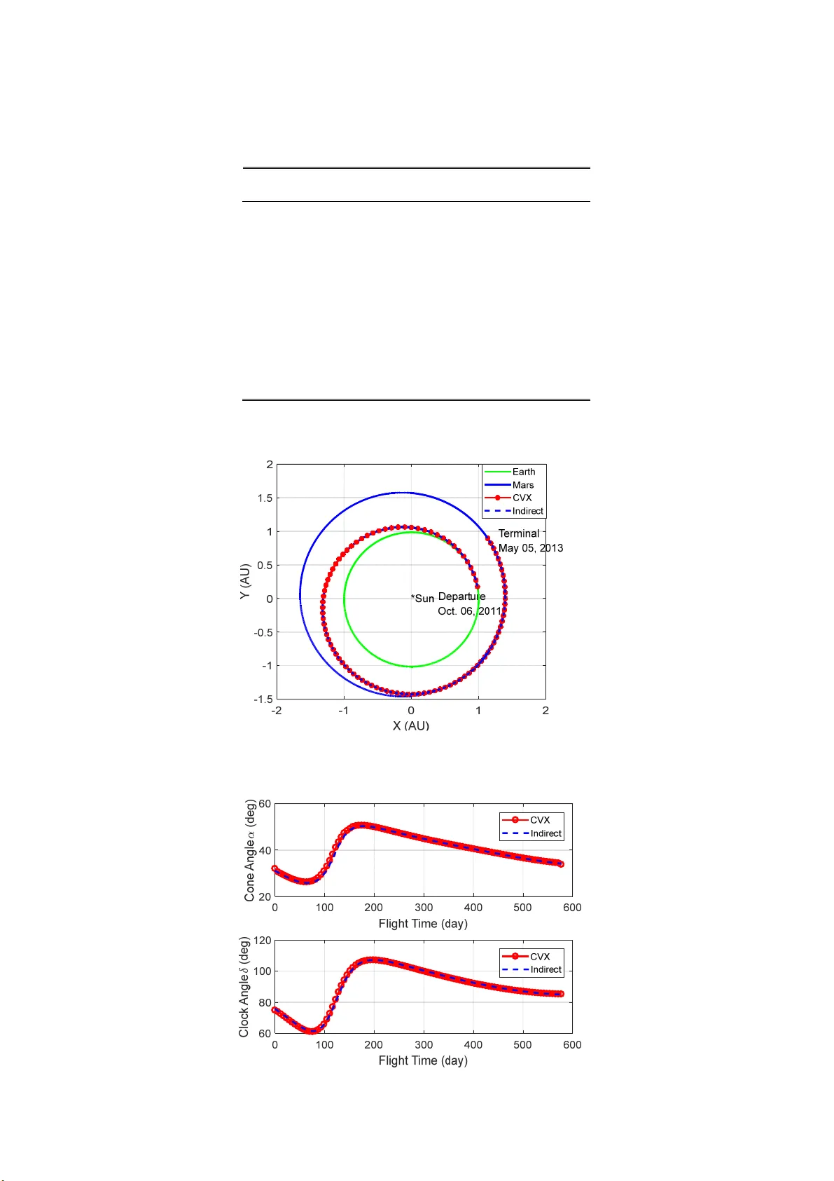
1 Solar -Sail Deep Space T rajectory Optimization Using Successive Convex Pr ogramming Y u Song, Shengpi ng Gong * School of Aerospace En gineering, T singhua University , Beijing, China Abstract: This paper presents a no vel methodolo gy for solving t he time-optimal trajectory optimization pr oblem for interplanetary solar -sail m issions using successive convex pro gramming. Based on the non-convex pr oblem, d ifferent convexificat ion technologies, such as change o f variables, successive lineariza ti on, trust re gions and virtual contro l, are discussed to convert the original problem into the formulation of successive convex programming. B ecause of the free final-time, successive linearization is performed iteratively f or the nonconve x terminal state const raints. After the convexification pr ocess, each of problems becomes a conve x prob lem, which can be solved effectively . A n augmented objective function is intr oduc e d t o e n s u r e t h e convergence performance and effectiveness of our algorithm. Aft er th at , al g ori th ms ar e designed to solve the discrete sub-pr oblems in a successive sol ution procedur e. Finally , numerical res ults demonstrate the effecti veness and accuracy of our algorithms. Key words: trajectory optimization, solar sail ing , successive convex optimization, direct method, indir ect method I. INTRODUCTION In d eep space, the solar radiation pressure force is one of the predominant perturbing forces exerted on the spacecraft. It can be utilized for orbit m aneuvers and t o achieve prop ellant-free interplanetary transfers. When a spacecraft utili zes solar radiation pressure as propulsion, it is called solar sailing. Early comparisons of solar sailing with chemical and ion propulsion s y s t e m s s h o w e d t h a t s o l a r s a i l s c o u l d match or outperf orm these system s for a range of mi ssion applic ations, though the level of assumed technology status is of course crucial in such comparisons (Mac Neal 1972). Af ter being studied for Corresponding author : S. Gong. Y . Song, Ph. D. student, Sc hool of Aerospace Engineering , T singh ua Uni versity ( yumai l201 1@16 3.com ). S. Gong, Associate professor , Sc hool of Aerospace Engi neering, T singhua University ( gongsp@tsinghua.edu.cn ). 2 several decades, a range of mission applications for solar sail ing were proposed, such as interplanetary travel (V ulpetti et al. 2015), space weather forecasting (Heili gers and Mcinnes 2014), planet sample return (Hughes et al. 2006), earth and lunar observation (Heili gers et al . 20 18), an d eve n appl ications for non-Keplerian orbits (Gong and Li 2015a; Heiligers et al. 2016; McInne s 1999; Song et al. 2016). The main fields of the study for solar sailing are divided into att itude maneuvers and orbit and trajectory design (Dachwald 2004; Gong and Li 2015b; McInnes 2004; Mengali and Quarta 2009; W ie and Murphy 2007; Zhukov an d Leb edev 1964) . W hen consid ering the trajector y design, the transfer time is usually minimized because of propellant- free p roperty of the so lar sail . Numerical methods for solving the optimization problem are basically d ivided into two major class es as indirect methods and direct methods ( R a o 2 0 0 9 ) . T h e i n d i r e c t m e t h o d r e q u i r e s t h e u s e o f t h e m a x i m u m principle to derive the first order necessary conditions of the optimal solution, which leads to a two-point boundary value problem and can be solved numerically , such as shooting method(Pontr yagin 1987) . As summarized by Bryson et al. (Bryson and Ho 1975), the main difficulty of this method is to find a first and accurate estimate of the initial unkno wn costate values that produces a solution reasonably clos e to the boundary conditio ns and first-order constraints, because the extremal solutions are oft en very sensitive to small changes of the initial constate valu es. On the other hand, a direct method usu ally discretizes the state and control of the problem in some manner and transforms the optimal contr ol probl em into a nonlinear progra mming problem (NLP), which has t he disadvantage of requiring a high n um ber of parameters for the discretization process (Betts 1 994; Margraves et al. 1987). Recently , convex programming has b ecome a popular method in the field of aerospace guidance, navigation and control (Liu et al. 2017). Because of th e mature theories and numerical algorithms, as well as the high computational ef ficiency and polyno mial comple xity , convex programming has been utilized in many applications in the aerospace field such as pl anetary and asteroids powered landing(Acikmese and Ploen 2007; Blackmore et al. 2010; Liu 201 7; Pinson and Lu 2016; Pinson and Lu 2015; Y ang et al. 2017), sp acecraft rendezvous and proximity operations (Liu and Lu 2013; Lu and Liu 2013), formation flight(Guo et al. 2 016; T illerson et al. 2 002) and spacecraft trajectory optimizati on(Harris and Açıkmeşe 2014; Liu et al. 2015; Zhang 2015). Considerable research h as been conducted for short-duration tr ajectory optimization and the ef fecti veness of convex programmi ng has been fully proved in comparison with traditional methods. For t he trans fer trajectory optimizat ion of low- thrust spacecraft, T ang (T ang et al. 2018) proposed a successiv e convex programming method and 3 provided an accu rate estimation of the initial costates of the indirect method. However , to the authors’ best knowledge, there is n o publication available in the litera tur e that addresses the convex programming for the optimization of solar -sail interplanetary transfer traj ectories. In this study , we explore the possibility of utilizing conv ex programming fo r the optimizatio n of a solar sail time-optimal transfer trajectory . Compared with the fuel-optimal and minimum-l anding- erro r problem s, the current problem has some new nonconvex elements because of the free final time. For the time-optimal problem, Harris (Harris and Açıkm eşe 2014) converted the minim um-tim e problem i nto a fixed final time probl ems and performed an outer loop to search for the optimal time. Y ang (Y ang et al. 2017) sol ved the reduced minim um-landing-er ror problem and com bined extrapolati ng and bi section methods to search for the minim um time of flight (TOF) for asteroid landing. Inspired by the free fin al time trajectory planning presented in the literature (Szmuk et al. 2016) that solves the fuel-optimal powered landing problem, dynamical equations of differentia l form will be used in this s tud y , and the time-related v ariables will serve as one of the o ptimization parameters, which means th e mi nimum-time problem will be solv ed directly without an outer loop. The rest o f the paper will be organized as follo ws. In Sec. II, the non-convex p roblem formulatio n is described. The dynam ic model and t he constraints o f a solar sai l spacecra ft are intr oduced and the time- optimal interplanetary transfer t rajectory problem is formulate d as a time-o ptimal control problem. In Sec. III, we adopt several methods to convert the or iginal non- convex problem into a sec ond-order co ne programmi ng (SOCP) formulat ion. In Sec. IV , algorithms are pres ented to guarantee the convergence property and the optimality . At last, numerical demonstrations will prove the validity of the method and the accuracy of the algorithms. II. NON-CONVEX PROBLEM FORM ULA TI ON In this section , we will present a basic model of the optimizat ion problem. W e consider the interplanetary transfer trajectory in deep space. In addition to the solar gravitation and the so lar radiation pressure force, there are many perturbati on forces influence th e m o t i o n o f t h e s o l a r s a i l , s u c h a s t h e gravity of nearby celestial bodie s, and the so lar wind (Da chwa l d and Wie 2005) . T o anal ysis the mission feasibility and verify th e proposed algo rithms, th e following s implifications as the literature are conducted in this study . The solar sail is assumed as a flat pl ate, and a perfectly reflecting force model is 4 adopted. Except th e solar gravitation an d the solar radiation p ressure forc e, other per turbation forces are neglected in this study . Moreover , it is assu med that the attit ude of the solar sail can be changed instantaneously . W e d efine the reference frame of the solar sail as follows. As shown in Fig. 1 , 𝒓  is the unit vector fro m the sun to th e sail , 𝒉  is t he unit vector al ong t he di rection of t he or bital angular m omentum vector and 𝒕  is the unit vector following from the right-handed reference f rame with 𝒓  and 𝒉  . The thrust of the solar sail originates from the reflection of the sunlight o ff the surface. The normal direction of the sail 𝒏  is described by two angles, the cone angle α and the clo ck ang le δ . As shown in Fig. 1 , the cone angle α is defined as the angle between the direction of the sunlight a nd the normal direction of the sail 𝒏  . The ang le para meter δ is the angle between the direction of the orb ital angu lar mo men tum and th e projection of 𝒏  on the plane perpe ndicular to 𝒓  . Thus , the expression of 𝒏  can be written as ˆ ˆ ˆˆ c o ss i n c o ss i n s i n       nr h t ( 1 ) The domains of the angles are as follows: [0, ], [0 , 2 ] 2     ( 2 ) Fig. 1 Definition of the re ference fr ame The acceleration of the sol ar s ail at a distance r from the sun can be written as: 2 2 ˆ cos s s r an    ( 3 ) where β is the l ightness num ber and μ s is the solar gravitational constant (McInnes 2004). In the heliocentric ecliptic inertial reference frame, the dyna mical equ ations of the solar sail Sun  δ Solar Sail 5 considering the solar radiation pressure acceleration in a two- body problem can be expressed as 3 s s r rv vr a          & & ( 4 ) As mentioned above, the TOF of the transfer trajectory is usual ly used as the perf ormance index of the optimal control problem because n o fuel is consumed by the sola r sail. Consider the interplanetary rendezvous problem of a sol ar sail. The solar sail is assumed t o leave the Earth with zero hyperbolic excess energy ( 𝐶  ≡0 k m 2 /s 2 ) and rendezvous with the tar get object (Mengali and Quarta 200 9). W ith the departure time at the starting planet being t 0 and the rendezvous time at the tar get object being t f , the initial and terminal state constraints can be described as: 00 0 00 () () () t t t       rr Ψ 0 vv ( 5 ) () () () ff f ff t t t        rr Ψ 0 vv ( 6 ) where  𝒓 󰇛 𝑡  󰇜 𝒗 󰇛 𝑡  󰇜  a n d 󰇩 𝒓𝑡   𝒗𝑡   󰇪 are the in itial and final states of the solar sail, 󰇣 𝒓 𝟎 𝒗  󰇤 a n d  𝒓 𝒇 𝒗   are the states of the departure and target cel estial bodies, respectively . Given the dynamical equations as in Eq.(1)-(4) and the constrai nts as in Eq.(5)-(6), the time-optim al control problem can be formulated as: Problem P0: 0 mi n . . Eq. ( 1 -6) f Jt t st  ( 7 ) As shown in Problem P0, the objective function is n on-convex an d the dynamical equations are highly non-convex. There fore, some conve xification techniques are need ed to ha ndle the probl em. III. CONVEXIFICA TION OF NON-CONVEX OPTIMIZA TI ON PROBLEM The optimizatio n problem as in Eq .(7) does no have the formulat ion of convex optimization, which m e an s t h at co n s i de ra b l e ef f o rt s a r e r eq ui r e d t o c on ve rt a n d d is cretize the problem into the framwork of SOCP and then a single or a sequence of convex optimizati on pro blems can be solved to approach the solution of the original optimizatio n problem(Liu et al. 2017). First, the change of control variables is adopted to reduce the coupling between the magnitude and direct ion of the solar radiation pressure 6 acceleration. Then, we formulate the differential dynamical equ ation s instead of the continuous-time ones. Usually , when the final time is free and if there is no a ppropriate alternative indepe ndent variable for continuo us-tim e dynamical equations, an outer loop t o searc h the optimal final time is necessary . The diffe rential dynamical equations have an obvious advantage in s olving this problem, in which the time interval can serv e as an optimization parameter considering a f ixed discrete number N . Additionally , we will apply successive convexification methods as introduced in (Liu and Lu 2014; Mao et al. 2017; Szmuk et al. 2016) to handle the non-conve x element s of the pro blem in the nonlinear dynamics and constraints. At last, the virtual cont rol method i s adopted to overcome the artificial infeasibility . A. CHANGE OF V ARIABLES As the only force for orbital maneuver, the acceleration of the solar sail shown as Eq.(3) consists of two parts: the magnitude and direction of the solar radiation p ressure force. The cone angle α appears in both parts, wh ich leads to difficulty o f the iterative conve rgence. Thus, we change the variables by equivalent t ransform ation and dec ouple the m agnitude a nd direct ion of the accelera tion as follows. Define the new control variables 𝒖≜ 󰇟 𝑢  𝑢  𝑢  󰇠  : 3 1 2 2 2 3 cos cos sin cos cos sin sin u α u αα δ u ααδ = = = ( 8 ) Then we can re write Eq. (1) and (3) as the followi ng form: () 12 3 2 ˆ ˆ ˆ s s μ β uu u r ar h t =+ + ( 9 ) Moreover , there exists an essential constraint Φ as follows, which is nonlinear and will be addressed in a later discussion. () 222 4 / 3 12 3 1 0 uuu u F =+ + - = u ( 1 0 ) B. DISCRETIZA TION For a specified number of time nodes N , the contin uous-tim e dy namical equations can be approximated to a discrete differential form. Fo r a given initi al time t 0 a nd f i n a l t im e t f , th e contin uous time domain can be replaced by a discrete time sequence from t 0 to t f . W e adopt the transform ation relationship introdu ced in (Szmuk et al. 2016) as fo llows. 7 0 1 1 f f tt t N kN - D= - -  ( 1 1 ) 0 0 , f tk t t k k éù =D + Î êú ëû ( 1 2 ) At the same time, the time interval Δ t will be an optimizatio n parameter instead of the final time t f considering a fixed initial time t 0 and discrete n umber N . For the discrete time sequence as shown above, the continuo us-t im e dynamical equations as Eq.(4) can be reformulated as a differential form at the discrete poin ts. The dynamics are d iscretized assuming that control parameters of solar radiation pressure acceleratio n are interpolated linearly between two adjacent time nodes. The discrete form of Problem P0 is shown a s Probl em P1 below , and the first two equations in Eq.(14) are in the s ame form as those in the literature (Szmuk et al. 2016). Problem P1: mi n Δ t ( 1 3 ) Subject to: () 2 2 11 [ 1 ] [ ] [ ] [ ] [ 1 ] [ 0, ] 32 1 [ 1 ] [ ] [ ] [ 1 ] [ 0, ] 2 ˆ [ ] [ ] [ ] [0, ] [] f f s s f kk k t k k t k k kk k k t k k μ kk k k k rk rr v a a vv a a ar a DD D æö ÷ ç += + + + + Î ÷ ç ÷ ç èø += + + + Î =- + Î ( 1 4 ) 0 0 [0] [0] éù - êú = êú - ëû rr 0 vv ( 1 5 ) [] ( ) [] ( ) ff f ff f kt kt éù - êú = êú - ëû rr 0 vv ( 1 6 ) Remark 1: 󰇩 𝒓  𝑡   𝒗  𝑡   󰇪 in Eq.(16) means that the terminal state constraints are chang ed when the final time t f is change d in the i terative process. The non-conve xity between th e term inal state and the optimization param eter , namely the state of t he tar get object a nd t he termi na l ti me t f will be addressed i n a later section. Remark 2: If there is no sp ecial explanation, th is paper will use k to represent the time nodes and i to represent the number of iterations. 8 C. SUCCESSIVE CON VEXIFICA TION In this section we will present a successive convexification pr ocedure to convert the problem discussed above to the SOCP formulation. W e perform the linearizatio n to the diffe rential dyna mics shown in Eq.(10) and Eq.(14 ). T rust reg ions are used to b ound the variab les involved in the linearization with the previous iteration. Unlike the state con straints in the literat ure (Szmuk et al. 2016), the terminal state constraints of our problem are time-varying and we will adopt t he forward integration method to approxim ate the terminal state during the iteration. Also, the virtual control mentioned in the literature will be adopted to handle the a rtificial in feasibility in the p revious several it erations. C.1 SUCCESSIVE LI NEARIZA TION There are two sources of nonlin earity in Problem P1 that can be linearized, the nonlinear dynamics Eq.(14) and nonlinear control co nstraints Eq.(10). Her e we defi ne a new variable fo rm as introduce d in (Szmuk et al. 2016): [ ] [ ] [ 1 ] 0, T TT rf kk k k k éù éù =+ Î êú êú ëû ëû Γ rr ( 1 7 ) where the subscript of the v ariable Г represents the type of the variable, for example Г r r epresents the position vectors at the k th and k+ 1 th nodes. Based on the previ ous definition, all the variables shown up in this problem can be written as the similar form : [] [] [] T TTT tk k k éù =D êú ëû rvu Γ ΓΓΓ ( 1 8 ) By adopting the successive li near ization method, the dynamics s hown in Eq.(14) can be reformulated as follows: ( ) ( ) 11 11 [ 1 ] [ ] [ ] [ ] [0 , ] [ 1 ] [ ] [ ] [ ] [0 , ] ri i f vi i f kk k δ kk k kk k δ kk k rr f Γ A Γ vv f Γ B Γ -- -- += + + ⋅ Î += + + ⋅ Î ( 1 9 ) wher e f r and f v are parts of the dynamics c ontaining the nonlinearity o f varia bles, A i-1 a n d B i-1 a r e t h e Jacobian matri x based on t he solutions of the i -1 th iteration. () () () 2 11 [] [] [] [ 1 ] 32 1 [] [] [ 1 ] 2 r v kk t k k t kk k t f Γ va a f Γ aa DD D æö ÷ ç =+ + + ÷ ç ÷ ç èø =+ + ( 2 0 ) 9 1 1 1 [] 1 [] i i r i k v i k - - - - ¶ = ¶ ¶ = ¶ Γ Γ f A Γ f B Γ ( 2 1 ) The nonlin earity in control constraints in Eq.(10 ) will also be successively satisfied by the following linearization. () 11 1 (, ) [ ] [ ] 0 ii i k δ k FF -- - =+ = uu u C u ( 2 2 ) where C i-1 is the Jacobian mat ri x of Eq.(1 0) based on the soluti ons u of the previous iteration as well. 1 1 [] i i k F - - ¶ = ¶ u C u ( 2 3 ) C.2 TR UST REGION The potential risk during lin earization is rendering the prob le m unbounded, and new states may deviate significantl y from the nominal state and control sequence (Mao et al. 2016; Szmuk et al. 2016), which increases the diffic ulty of converge nce severely and possibly l eads to infeasibility of the lin earized problem . T o avoid this ris k, the trust regions are adopted t o c onstrain the variables as follows: u δη £ u ( 2 4 ) 2 t δ t η D D£ ( 2 5 ) where η u a n d η Δ t are trust regio n radius th at restricts the control inputs and time interval in ev ery iteration and will be penalized via additional terms in the augmented obj ective function. In the first few iterations, the trust region radius can be appropriately larger to find a p roper convergence direction. Wit h the increase of iter ations, the trus t region radius should be gradu ally narrowed considering the convergence and validity of th e linearized problem. Remarkably , as long as the control inputs u a n d t i m e i n t e r v a l Δ t a r e c o n s t r a i n e d , t h e n e w s t a t e s , n a m e l y the position and ve locity vector s can be constrained as well du e to the linearized dynamic equations. C.3 TERMINAL ST A TE CONSTRAINTS In the previous literature, most of the terminal state constrai nts are time independent or in simple mapping relationship. For our problem, the constraints of termi nal state as Eq.(16) are time-varying because of the integration of tim e. These highly nonlinear cons traints can not be applied directly in a 10 convex optimizatio n procedure wh en regarding the final time as an optim ization parameter . Existing literature mainly considers the fin al time fix ed in an iteratio n and update the final time at the end of every iteration (Ha rris and Açıkmeşe 2014; Y ang et al. 2017 ). Considering a small variatio n range of the terminal time, which is reasonable under the constraint of trust region of time, the state of the target object varies sli ghtly near the previous state. Therefore, we can use the forward integrati on method to approximate the new state changed because of the small time variation δ t f . W e define the state of the target object as 𝒙  󰇣 𝒓  𝒗  󰇤 , wher e r ter a n d v ter indicate th e position and velocity of the target object. Th e state of the tar get object c an be a pproximate d as follows. () ( ) ter ter ter ter 2 ter ter , ter , 1 , 1 ter , 1 , 1 , ( ) () () f ii f i i f i f i μ r tt t δ t v xg x r xx g x -- -- éù êú êú == êú - êú ëû =+  ( 2 6 ) where the nonlinear function g represents the two-bo dy motion equation of the target object, 𝒙 ,  󰇛𝑡 , 󰇜 is the nominal terminal state calculated accurately using the obtained terminal time t f,i- 1 from the pre vious i teration. Remark : T o avoid the error accum ulation caused by the approxim ation, th e no minal te rminal s tate needs to be updated every itera tion as long as the terminal tim e t f, i is obtained in t he i th iteration. C.4 AUGMENTED OBJ ECTIVE FUNCTION Considering the linearizat ion and trust regi ons ad opted to our problem, the ob jective func tion Eq.( 13) in Problem P1 is apparently insufficient. T o ensure the converg e nce performance and the effective ness of our algori thm, take i nto account the augmented o bjective fun ction as follows: mi n tt tw η w η DD D+ ⋅ + ⋅ uu ( 2 7 ) where η u and η Δ t are trust regi on radius m entioned pre viousl y and w Δ t and w u are the penalty parameters respectively , which will be updated by a classical L1 penalty m ethod (Nocedal and Wri ght 2006). D. AR TIFICIAL INFEAS IBILITY Because of t he linearization a nd state constraints mentione d pr eviously , infeasibility occurs in the first few iterations and ob structs th e iterative process, namely artificial infeasibility (Mao et al. 2016). Th ere 11 are several methods of dealing with the problem. One is t o rela x some of t he constraint s, such as t erminal constraints, and penalizi ng the relaxing radius in the augm ente d objective function (Liu e t a l . 20 1 5 ) . Fo r our problem consideri ng a free te rminal time, relaxed terminal constraints mean more algorithm complexit y . Another com monly used metho d is vi rtual cont rol (Ma o et a l. 2016; Szmuk et al. 201 6). W e introduce an additiona l accel eration term a v into the dy namical equat ions as the vi rtual control i nput: 2 ˆ s s v μ r ar a a =- + + ( 2 8 ) Then we furt her augm ent the objective function a s follows: mi n v tt v tw η w η w uu a a DD D+ ⋅ + ⋅ + ⋅ ( 2 9 ) where w a v is a heavy penalty factor for the m agnitude of virtual contr ol input . The virtual contr ol input a v is significant at the first few iterations to prevent the arti ficial infeasibility and will ap proach zero after several iterations because of the heavy penalty in the objective function . Namely , the virtual con trol input will not make the solu tion de viate from the original problem while increasing the problem’s co nver gence performance. After t he successive conve xification processes, we obta in the f ollo wing c onvex optim ization problem configuratio ns as Problem P2. The algorithms and numerical demonstration discussed in the following sections are ba sed on the f ormulat ion of Problem 2. Problem P2: Objective Function: mi n v tt v tw η w η w DD D+ ⋅ + ⋅ + ⋅ uu a a ( 3 0 ) Boundary Condition s: 0 0 [0] x éù êú = êú ëû r v ( 3 1 ) () () ter , 1 ter , 1 1 fi f i f i kk k δ tN xx g x -- éù éù éù =+ D ⋅ - êú êú êú ëû ëû ëû ( 3 2 ) Dynamics: [] [] [] T TTT tk k k éù =D êú ëû rvu Γ ΓΓΓ ( 3 3 ) () () 11 11 [ 1 ] [ ] [ ] [ ] [0 , ] [ 1 ] [ ] [ ] [ ] [0 , ] ri i f vi i f kk k δ kk k kk k δ kk k -- -- += + + ⋅ Î += + + ⋅ Î rr f Γ A Γ vv f Γ B Γ ( 3 4 ) 12 2 ˆ [ ] [ ] [ ] [ ] [0 , ] [] s s vf μ kk k k k k rk =- + + Î ar a a ( 3 5 ) () () () () 2 11 1 1 [] [] [] [ 1 ] 4 1 [] [] [ 1 ] 2 ri i vi kk t k k t kk k t f Γ va a f Γ aa DD D -- - =+ + + =+ + ( 3 6 ) Control C onstraints: 1 2 3 0 1 11 11 u u u ££ -£ £ -£ £ ( 3 7 ) 1 (, ) 0 i F - = uu ( 3 8 ) IV. SUCCESSIVE SOLUTION PR OCEDURE In this section, we will propos e the successive solution proced ure to find the solution of the optimal control problem by solving the convex problem iteratively . For the first iteration, we need provide an initial reference solu tion for the iterative process. Many work s in the literature h ave shown that the successive solution method is in sensitive to the in itial refere nce solution(Mao et al. 2017; Szmuk et al. 2016). W e will illustrate this performance in the next section. In our successive solution procedure, the i th so lution is used to approximately linearize the n onlinear dyna mics and constraints in the i +1 th iteratio n. T o guarantee the convergence of the iterative process, a kind o f quadratic penalty method is adopted to update the penalty parameters. W e perform the process repeatedl y until the conv ergence criteria is satisfied. The procedure is stated in Algorithm 1. Algorithm 1 Successive Solution Algorithm Step 1 : Select an initial reference solution 󰇝 𝒙  ;𝒖  󰇞 * . Specify the initi al guess of the terminal time 𝑡 , and compute ∆𝑡  using the discrete number N ; Step 2 : Initialize the weight coefficients 𝑤 ∆ ,𝑤  ,𝑤    . Step 3: Perform the first itera tion and get the solution x 1 , u 1 and Δ t 1 . Update t he weight coefficients 𝑤 ∆ ,𝑤  ,𝑤    . Step 4 : For the i th iteration, update the re ference result with the i -1 th iteration solution x i- 1 , u i -1 and Δ t i -1 and solve Problem 2; Step 5 : If ‖ 𝒖  𝒖  ‖ ε  a n d | ∆𝑡  ∆ 𝑡  | ε ∆ , 13 return 󰇝 𝒙  ;𝒖  ;∆ 𝑡  󰇞 as the result of Problem P2; else Update 𝑤 ∆ ,𝑤  ,𝑤    ; i = i +1; and back to Step 4 ; end Step 6 : If i ≥ i max , return “Infeasible” for the problem. * The subscript of 𝒙  and 𝒖  indicate the initial reference solution for the first iteratio n. V. NUMERICAL TEST CASES In th is section, we will intro duce the n umerical r esults and de monstrate the effectiveness and robustness of the proposed algorithm for solar sail transfer tr ajectory optimization. T o de monstrate the effective ness of our method, the e xisting m ethods such as the i ndirect method and the direc t pseudospectral method will be used to solve the same cases for comparison. Guaranteed by the first order necessary conditions, solutions of indirec t m ethods are conside red as the local opt imal solutions. Repeatedly solved solution s of th e indirect method are c onsider ed as the global optim al solutions (He et al. 2014). In a ddition, the di rect pseudospect ral method has be en widely used for sol ar sa iling trajectory optimization in the literature (Heiligers et al. 2 015; Melto n 2 002). For th e verificatio n of the effectiveness, accuracy and optimality of the pro posed algorithm, solutions ob taine d by the i ndirect met hod and direct pseudospectral m ethod are referenced a nd compared with the sol u tion of c onvex programmi ng. T o verify the ro bustness of the proposed algorithm, different i nitial guesses of the terminal time will be set and the results will be c ompared to illustrate the conve rgence properti es of the algorit hm. Moreover , test cases that have been studied abundantly in the l iterature, such as the rendezvous problem with Mars and asteroid Apophis (Hughes et al. 2006; Men gali and Qu arta 2009), will be considered to verify the applicability an d effectiveness of the proposed meth od. A. SELECTION OF CELESTIAL BODIES AND P ARAMETERS W e consider the orbit transfer trajectories from Earth with zer o hy perbolic excess ener gy and the time to leave the Earth is f ixed. The characteristic acceleration of t h e s o l a r s a i l i s s e t t o a c = 0 . 5 m m / s 2 14 (correspondi ng to a lightness number of β =0.0843), which is reasonable and widely used in the literature (Hughes et al. 2006; Meng ali and Quarta 200 9). For the sake of computational efficiency , all distance quantiti es ar e n or ma li ze d w it h t he a st ro nom i ca l unit (AU) and time-related quan tities are normalized with 1/2𝜋 year . The reference orbit elements from JPL’s database † at MJD 57800 are listed in T able 1 . T able 1 Reference or bit elements of aster oids a (AU) e i (rad) Ω ( r a d ) ω ( r a d ) M (rad) Earth 0.9995 0.0166 0.0000 3.5798 4.4677 0.7822 V e nus 0.7233 0.0067 0.0592 1.3375 0.9602 6.1 517 Mars 1.5237 0.0935 0.0322 0.8640 5.0032 1.0011 Apophis * 0.9222 0.1911 0.0581 3.5684 2.2060 3.7619 * The reference orbital elem ents of asteroid Apophis are defined at Modified Julian Date (MJD) 54441 T o use the successive solution method for convex programming, t he initial reference values of the iterative process need to be speci fied. As described in the pre vious section, the initial reference solu tion can be selected roughly and will not affect the convergence per formance. Hen ce, the initial reference state variables are chosen as the state variables of the initia l celestial body and the control angles are specified as constants, for example 𝛼 ≡ 30° a n d 𝛿 ≡ 180° . Another initial reference variab le n eeds to be specified is the terminal tim e. Once the time of departure t ime is determined, the guess of the final time will be estimated conservatively accord ing to the differen c e o f t h e o r b i t a l e l e m e n t s a n d t h e performance of the solar sail . For the indirect method, the original optimal control problem w ill be converted to a two-point boundary value problem and will be so lved by shooting method. T he initial guess of the un known values are randomly generated un til the final converg ence. For the d ir ect pseudospectral method, the initial guesses will be set to the same as those of the convex optimiza tion. The MA TLAB software CVX, a packag e for specifying and solving c onvex p rograms (Grant and Boyd 2015), will be u sed an d the solver ECOS (Domahidi et al. 2013) is called in our numerical test cases. When performing the indirect shooting procedure, MinPack-1 (Mor é et al. 1980), a package of Fortran subprogram s for the numerical solution of systems of nonlinear equations and nonlinear least squares problems is used. In addition, the general-purpose software GPO PS (Rao et al. 2010) for solving optimal † Data availabl e online at https://ssd.jpl.nas a.gov/dat/ELEMENTS .NUMBR [retrieved 22 Februar y 2017]. 15 control problems will be used to obtain results of the d irect p seudospectral method. All the numeri cal computati ons are exe cute d on a P C wit h an In t el Core i7-4470 at 3.4GHz and 8GB of mem ory . B. NUMERICAL RESUL TS B.1 RENDEZV OUS WITH MARS As first test case, we consider the transfer mission from Earth to Mars. The departu re time is fixed to MJD 55840 (Oct. 06, 201 1), which is the same as the case in the literature (Hughes et al. 2006). In this case, a value of N =100 is used for the d iscretizati on described in Sec. III.A. Th e value of other parameters used for this case are listed in T ab le 2 . T able 2 Numerical Simulation Parameter s Parameter V alue Units 𝑡  55840 MJD 𝑡 , 56140 MJD 𝛽 0.0843 - N 100 - 𝜂 , 0.5 - 𝜂 , 10 day 𝑤  0.1 s -1 𝑤  0.01 - 𝑤  7 11 0 ´ - 𝜀  5 11 0 - ´ - 𝜀  3 11 0 - ´ day For the given departure time at Earth, the solar sail rendezvou se s w i t h M ar s o n M ay 5 2 0 1 3, an d t he TOF is 577.591 days. The result is consistent with the results in the literature (Hughes et al. 2006), which verifies the optimali ty of the proposed method. The indire ct me thod is used to solve the problem with then same boundary conditions for com parison. The res ults obtai ned by successiv e convex programming and indirect method is as T a ble 3, Fig. 2 and Fig. 3. 16 Ta b l e 3 Conve rgence Solution of th e Mars Rendezvous Pr oblem Description Result Number of iterations 16 Departure d ate 10-06-2011 TOF (day) 57 7.391 Rendezvous date 05-05-2 013 Iteration err or of control 3.61×10 -5 Rendezvous error(AU) 1.22×10 -9 Fig. 2 T ra nsfer traj ectory of Mars rendezvous 17 Fig. 3 Contr ol profiles o f Mar ren dezvous The parameters listed in T able 3 represen t the results of th e solution ob tained using conv ex programming. The initial g uess for the TOF is 300 days. The con ver gence criterion we used is the iteration error that represents th e error of the control variab les between two adjacent iterations. The algorithm converges a fter 16 tim es iteration. After we obtain t he soluti on, the reinte gration proce dure is con d uct ed t o v er ify t he sol utio n. T he di f fe renc e i n t he st at e v ariables between the solar sail and Mars at the time of rendezvous after reintegr ation is of 1.22×10 -9 no rmalized time unit, which ind icates th at th e obtained sol ution by c onvex optim ization is val id and accur ate enough. Compared to the solution obtained with the indirect method, the T OF obtaine d by convex programmi ng is slight ly longe r because of the discreti zation error . The posi tion and velocity of the solar sail in the transfer trajectory is basically in agreem ent with the result of t he i ndirect m ethod, as shown in Fig. 2 . The control angles of the sola r sail are also consistent with the results of the indirect method shown as Fig. 3 . The numerical r esults above conf irm the effectiveness an d optim ality of the proposed alg orithm for convex programm ing. In the next section the conver gence and rob ustness performance will be discussed by changing the simulation p arameters in different conditions. B.2 RENDEZVOUS WITH ASTEROID ASTEROIDS T o demonstrate the efficiency of the proposed method, the direc t pseudosp ectral method w ill be adopted for com parison. In th is case, the asteroid 99942 Apophi s is chosen as the target object. T he time of d eparture is set as MJD 56 258 (Nov . 27, 2012) according to t he test case in ano ther literature (Mengali and Quarta 2009). For the given time of departure time, the sol ut ions obt ained by convex pr ogramm ing and direct pse udospectral m ethod are as T able 4, Fig. 4 a nd Fig . 5. T able 4 Convergence Solution of the Apophis Rendezvous Pr oblem Description Result CVX GPOPS Number of iterations 16 20 TOF (day) 279.912 279.945 18 Effective computation time (second) 0 .960 28.240 Fig. 4 T ransfer trajectory of Apophis ren dezvous Fig. 5 Control profiles of Apophis rendezvous The initial referen ce and bound ary conditions are set to the sa me situation of the two methods. The results and comput ation tim e of each m ethod are rec orded. As sh own in Ta b l e 4 , the results for the T OF obtained by conve x o ptimiz ation an d di rect pseudospectral m etho d are almost i dentical except for minor error . The trajectory in Fig. 4 a n d t h e c o n t r o l p r o fi l e s i n Fig. 5 indicate that the results of the different method are c oincident. C ompared wi th the di rect method, t he pro pose d method a re more ef ficient . B.3 RENDEZV OUS WITH VENUS In this case, we select the V enus as the target object. T o veri fy the conver gence and robustness performance of the proposed algorithm, different conditions a re set for further discussion in this case. 19 The solution obtained by convex programming is as follows. The solar sail d eparture from the Earth on October 26 2019 and rendezvouses with V enus on Augu st 02 2020, correspond ing to a TOF of 281.167 days. The t ransfer trajectory a n d control profiles are s hown in Fig. 6 and Fig. 7 . Ta b l e 5 Conver gence Solution of the V enus Rendezvous Problem Description Result Number of iterations 12 Departure time 10-26-2019 TOF (day) 28 1.167 Rendezv ous T ime 08-02-2 020 Fig. 6 T ransf er traje ctory of V enus rendezvous Fig. 7 Control profiles of V enus r endezvous 20 Fig. 8 Iterative pr ocess of e quivalent contr ols Fig. 9 Magni tude of virtual contr ol and iterati on err or i n the iterati ve proce ss In this case, we output the iterative process for the illu strat ion of the converge nce performance. The curves in Fig. 8 illustrate the iterative process of the equivalent control def i n e d in E q . ( 8 ) . A s s h o w n i n Fig. 8 , different co lor lines represent different iterative times and the red-dotted lin e represents the optimal convergence solution. For a sequence of arbitrarily giv en initial reference con trols, the convergence results w ill finally c onverge to the optimal soluti on, which illustrates the robu stness o f the proposed al gorithm. The fir st curve of Fig. 9 illustrates the magnitude of the virtual control and the secon d cu rve expresses the variation o f the iteration errors along with the iterations . In the f irst few iteration s, the iterative process would be infeasible because of artificial infeasibility and we make a compensation with virtual control. Our greatest concern is whether the e xistence of virtual contro l will af fect the authenticity of the original 21 problem. It is obvious judging from Fig. 9 that the virtual control makes contribution only in the first two iterations and tends to zero later because of the heavy penalty in the objective functio n in Eq.(30). Moreover , according to the variation of the iteration errors in the second curve of Fig. 9 , convex programming with the proposed algorith m shows a good convergenc e performance. Fig. 10 Convergence performance of di ffer ent initial guesses o f T OF 0 For further discussion, differen t initial guesses for the TOF a re speci fied. The lines i n Fig. 10 show the convergence performance of dif ferent initial guesses for th e T OF . The guesses for T OF are specified from 100 days t o 1 year and the final conve rgence s le ad to the same v alue of 281 .167 day , which illustrates the robustness of the convex p rogramming with the proposed algorithm. VI. CONCLUSION The successive convex programming is investigated in this paper to solve the transfer trajector y optimization of solar sail. Dif ferent convexification technolog ies, such as cha nge of variable s, successi ve convexification, and virtual control, are adopted to conv ert th e original problem into the formulation of convex progra mming. W e present a standar d successive c onvex app roac h to s olve a se quence of c onvex sub-problems and obtain the op timal solution ultimately . Nu meri cal test cases dem onstrate the effectiveness and accuracy of th e proposed algor ithms. By introdu cing the test case from the literature, the op timality o f the obtained solution is guaranteed. The resu lts of the reintegration indicate the accuracy and v alidity of the solution. Compared with the traditional dir ect method, such as pseudospectral method, the proposed method is more efficiency . Diffe rent conditions of the initial guesses are considered in the 22 test case. W ith different initial guesses for TOF , the algorith m has the sam e conver genc e solut ion, w hich illustrates the robustness of the proposed algo rithm. VII. ACKNOWL EDGMENTS This work i s support ed by the Na tional Natural Science Foundati on of China (Gr ant No. 11772167). 23 REFERENCE Acikmese, B., Ploen, S.R.: Convex Progra mming Approach to P owe red Desce nt Guidance for Mar s Landing. J. Guid. Contro l. Dyn. 30, 1353–1366 (20 07). doi:10.25 14/1.27553 Betts, J.T.: Optimal Inter planet ary Orbit Transf ers by Dir ect Transcription. J. Astronaut. Sci. 42, 247– 268 (19 94) Blackmore, L., Acikm ese, B., Scha rf, D.P.: Minim um-Landing-Err or Powered-Desce nt Guidance for Mars Landi ng Using C onvex Opti mization. J. Guid. C ontrol. Dy n. 33, 1161–1171 (201 0). doi:10.2514 /1.47202 Bryson, A.E., Ho, Y.C.: Applie d optim al control. Hem isphere Pu blishing, New Yor k (1975) Dachwald, B .: Optim ization of I nterplaneta ry Solar Sailcraft T rajectori es Using Evolutiona ry Neurocontrol. J. Gu id. Control. Dyn. 27, 66– 72 (2004). doi:10 .2 514/1.928 6 Dachwald , B., Wie, B.: Solar sail trajectory optimization fo r intercepting , impacting, and deflecting near-earth asteroi ds. AIAA Guid. Na vig. Control Conf. Exhib. pa per 2005-6176 (200 5). doi:10.2514 /6.2005-6176 Domahidi, A., Chu, E., Boyd, S.: EC OS: An SOCP solver for embedded system s. Proc. Eur. C ontrol Conf. 3071–307 6 (2013). doi:10.0/Linux -x86_64 Gong, S., Li, J.: Equilibria near asteroids for solar sails wi th reflection contro l d evices. Astrophys. Space Sci. 355, 213–223 (2015)(a). doi:10.10 07/s10509-014-2165- 7 Gong, S., Li , J.: A new i nclination cra nking method for a flex ible s pinning solar sail. IEEE T rans. Aerosp. Electro n. Syst. 51, 2680–2696 (2015 )(b). doi:10.1109/TA ES.2015.1 40117 Grant, M.C., Boyd, S.P.: The C VX Users’ Guide, Release v2.1. B ook. (2015). doi:10.1.1.23.5133. Guo, J., Chu, J., Yan, J.: Establishm ent of UAV formation flig ht using cont rol Vector parameterizat ion and sequenti al convex program ming. Chi nese Con trol Conf. CCC. 2016–Augus, 2559–2564 (2 016). doi:10.1 109/ChiCC.2016.7553 749 Harris, M.W., Açıkm eşe, B.: Minimum Time Rendezvous of Multipl e Spacecraft Using Differential Drag. J. Guid. Con trol. Dyn. 3 7, 365–373 (2014). doi:1 0.2514/1. 6150 5 He, J., Gong, S., Jiang, F.H ., Li, J.F.: Time-optim al rendezvo us transfer trajecto ry for restricted cone- angle range solar sails. Acta Mech . Sin. Xuebao. 30, 628–635 (2 014). doi:10 .1007/s10409-014 -0033-x Heiligers, J., Macdon ald, M., Par ker, J.S.: Extension of Earth -Moon libration po int orbits with solar sail propulsion. Astrophys. Space Sci. 361, (2016). doi:10.1007 /s10509-016-2 783-3 Heiligers, J., Mcinnes, C.R.: Nov el solar sail mission concept s for space weather forecasting. Adv. Astronaut. Sci. 15 2, 585–604 (201 4) Heiligers, J., Mingo tti, G., McInnes, C.: Optimisation of sola r sail interplaneta ry heteroclin ic connections. In: Advances in th e Astronautical Sciences. pp. 21 1–230 (2015) Heiligers, J., Parker, J.S., Macd on ald, M.: Novel Solar-Sail M ission Concep ts for High-Latitude Earth and Lunar Observ ation. J. Guid. Control. Dyn. 41, 21 2–230 (2018 ) . doi:10.2514/1.G00291 9 Hughes, G.W., Macdonald, M., McI nnes, C.R., Atzei, A., Falkne r , P.: Sam ple Return from Mercury and Other Terrestrial Planets Using S olar Sail Propulsion. J. S pacecr. Rockets. 43, 828–835 (2006). doi:10.2514 /1.15889 L i u ， , X., Shen ， , Z., Lu, P.: Solving the Maxim um-Crossrange Problem via Succes sive Second Order Cone P rogramming. Aerosp. Sci. Technol. 47, 10–20 (2015 ) Liu, X.: Fuel-Optimal Rocket La nding with Aerodynamic Contro ls . In: AIA A Guida n ce, Navigation, and Control Co nference (2017) Liu, X., Lu, P.: Robust Trajecto ry Optim ization for Highly Con strained Rendez vous and Pr oximity 24 Operations. AIA A Guid. Navig. Control Conf. (201 3). doi:doi:10. 2514/6.2013- 4720 Liu, X., Lu, P.: Sol ving Non convex Opt imal C ontrol Pr oblems by Convex Optimization. J. Guid. Control. Dyn. 3 7, 750–765 ( 2014). doi:10.251 4/1.62110 Liu, X., Lu, P., Pan, B.: Sur vey on Convex Optimization in Aer ospace Applications. Astrodynamics. 1, 23–40 ( 2017). doi:10.100 7/s42064-017- 0003-8 Lu, P., Li u, X.: Autonom ous Traject ory Planni ng for Rend ezvous and P roximit y Operations by C onic Optimi zation. J. Guid . Control . Dyn. 36, 375–389 (2013). doi :10 .2514/1.58436 MacNeal, R.H.: Compar ison of the Solar Sail with Electric Prop ulsion Systems,. Comp. Sol. Sail with Electr. Propuls. Syst. (1972) Mao, Y., Dueri, D., Szmuk, M., Açı km eşe, B.: Successive Convex ifi cation of N on-Conv ex Optim al Control Pr oblems wi th State Const raints. IFAC-Pa persOnLine. 50, 4063–4069 (2017 ). doi:10.1016 /j.ifacol.2017.08.789 Mao, Y., Szmuk, M., A cikmese, B.: Successi ve conve xification o f no n-convex optima l control problem s and its converge nce properti es. 2016 IE EE 55th Con f. D ecis. Control. CDC 2016. 363 6–3641 (2016). doi:1 0.1109/CDC.2 016.7798816 Margraves, C .R., Paris, S.W., Ha rgraves, C.R.: Direct Tra jecto ry Optimization Using Nonlinear Programming and Collocation. J. Gu id. Contr ol. Dyn. 10, 338–3 42 (1987). do i:10.2514/3.20223 McInnes, C.R.: Sola r sail missi on appli cations for non-kepleri an orbits. Acta Astronau t. 45, 567–575 (1999). doi:1 0.1016/S0094-57 65(99)00177-0 McInnes, C.R .: Solar Saili ng: Technology , Dynam ics and Mission Applications. Springer (2004) Melton, R.: C omparison of direct opt imization m ethods ap plied to s olar sail problem s. AIAA Pa p. (2002) Mengali, G ., Quarta, A .A.: Rapid Solar Sail Ren dezvous Missio n s to Astero id 99942 Apophis. J. Spacecr. Rockets. 46, 134–140 (2009). doi:10. 2514/1.37141 Moré, J.J., Garbow , B.S., Hillstrom , K.E.: User Guide for MINP ACK-1, http://cdsweb.cern.ch /record/126569, (1980) Nocedal, J., Wright, S.J .: Numeri cal optimization. S pringer Se ries in Operations Research and Financial Engi neering (2006) Pinson, R ., Lu, P.: R apid Generat ion of Ti me - Optim al Traject ories for Asteroid Land ing via Convex Optimi zation. Am. Ast ronaut. Soc. 1–19 (20 15). doi:1 0.2514/1.G 0 02170 Pinson, R., L u, P.: Trajectory Design Employing Convex Optimiz ation for Landing on Irregularly Shaped Aster oids. In : AIAA/AAS A strodynamics Specialist Confere nce. pp. 1–22 (2016) Pontryagi n, L.S.: Mathem atical theory i n optimal control proce ss. CRC Press (1987) Rao, A. V.: A survey o f numerical m ethods for optimal control. Adv. Astronaut. Sci. 135, 49 7–528 (2009). doi:1 0.1515/jnu m-2014-0003 Rao, A. V., B enson, D.A., Darby, C.L., Patterson, M.A., Sander s, I., Huntington, G.T.: GPOPS: a MATLAB software for solving multiple-phase optimal control prob lems using the Gauss pseudospectral method. ACM Trans. Math. S oftw. 37, (20 10) Song, M., He, X., He, D.: Displ aced orbits for sola r sail equi pped with reflectance control devices in Hill’s restricted three-body pro blem with oblateness. Astrophys. Space Sci. 361, (2016). doi:10.1007 /s10509-016- 2915-9 Szmuk, M., Acikm ese, B., Berning , A.W.: Successi ve Convexifica tion for Fuel-Optimal Powered Landing with Aerodynamic D rag and Non-Conv ex Constraints. AIAA Guid. Navig. Control Conf. 1– 16 (2016). do i:10.2514/6.2016-03 78 25 Tang, G., Jiang, F., Li, J .: Fuel-Optimal Low-T hrust Trajector y Optimization Using Indirect Method and Successive Co nvex Progr amming. IEEE Trans. Aeros p. Electron . Syst. 9251, 1–1 (2018). doi:10.1109 /TAES.2018.2803558 Tillerson, M., Inalha n, G., How, J.P.: Co-ordination and contr ol of distributed spacecraft system s using conve x optim ization techni ques. Int. J. Robust Nonlinear Control. 12, 207–242 (2002). doi:10.1002/rnc.68 3 Vulpetti, G., Johnson, L., Ma tlo ff, G.L.: Solar Sail: A Novel Approach to Interplanetary Travel. Springer, New York (2015) Wie, B., Murphy, D. : Solar-Sail Attitude Control Design for a Flight Validation Mission. J. Spacecr. Rockets. 44, 809–821 (2007). doi:10.2 514/1.22996 Yang, H., Bai , X., Baoyin, H.: R apid Ge neration of Time-Optima l Trajectories for Asteroid Landing via Convex Optimization. J. G uid. Control. Dyn. 40 , 628–641 (20 17). doi:10 .2514/1.G00217 0 Zhang, S.J.: Conv ex Programming Approach to Real- time Trajecto ry Optimization for Mars Aerocapture. Aerosp. C onf. 2015 I EEE. (2015) Zhukov, A.N., Lebedev, V.N.: V a riational Problem of Transfer B etween Heliocen tric Orbits by Means of Solar Sail. Cosm . Res. 2, 41–44 (1964)