Convergence Properties of the Heterogeneous Deffuant-Weisbuch Model

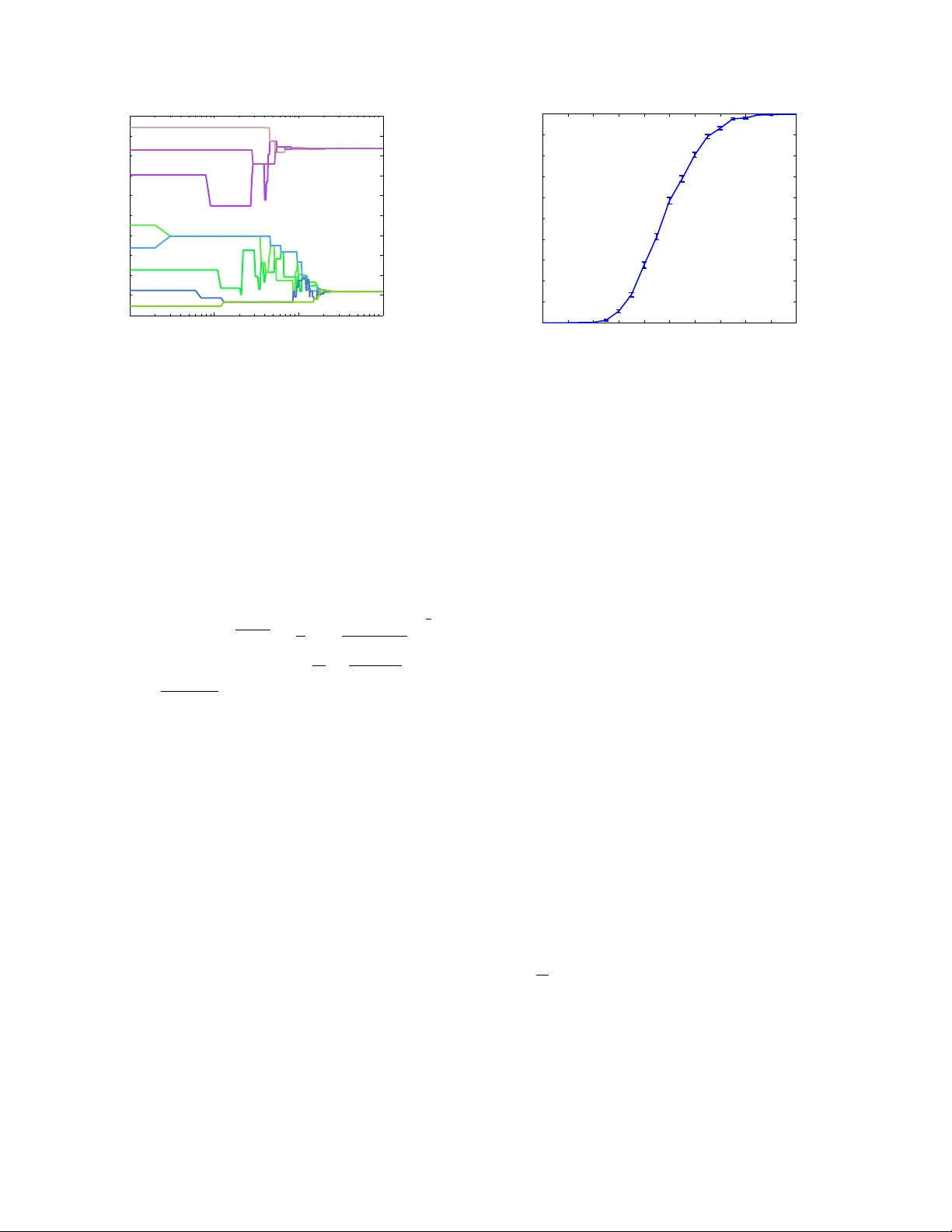
Con v ergence Prop erties of the Heterogeneous Deffuan t-W eisbuc h Mo del ? Ge Chen a , W ei Su b , W enjun Mei c , F rancesco Bullo d , a National Center for Mathematics and Inter disciplinary Scienc es & Key L ab or atory of Systems and Contr ol, Ac ademy of Mathematics and Systems Scienc e, Chinese A c ademy of Scienc es, Beijing 100190, China b Scho ol of Automation and Ele ctric al Engine ering, University of Scienc e and T e chnolo gy Beijing, Beijing 100083, China c Automatic Contr ol L ab or atory, ETH, 8092 Zurich, Switzerland d Dep artment of Me chanic al Engine ering and the Center of Contr ol, Dynamic al-Systems and Computation, University of California at Santa Barb ar a, CA 93106-5070, USA Abstract The Deffuan t-W eisbuc h (D W) model is a b ounded-confidence opinion dynamics model that has attracted m uch recent interest. Despite its simplicit y and app eal, the DW model has prov ed technically hard to analyze and its most basic con vergence prop erties, easy to observe numerically , are only conjectures. This pap er solves the conv ergence problem for the heterogeneous DW model with the weigh ting factor not less than 1 / 2. W e establish that, for an y p ositive confidence bounds and initial v alues, the opinion of each agent will conv erge to a limit v alue almost surely , and the conv ergence rate is exp onential in mean square. Moreo ver, w e show that the limiting opinions of an y tw o agents either are the same or hav e a distance larger than the confidence bounds of the tw o agents. Finally , we provide some sufficient conditions for the heterogeneous DW model to reac h consensus. Key wor ds: Opinion dynamics, consensus, Deffuant mo del, gossip mo del, b ounded confidence mo del 1 In tro duction The field of opinion dynamics studies the dynamical pro- cesses regarding the formation, diffusion, and evolution of public opinion ab out certain even ts and ob ject of in- terest in so cial systems. The study of opinion dynam- ics can b e traced back to the tw o-step communication flo w mo del in ( Katz and Lazarsfeld , 1955 ) and the so- ? This w ork w as supp orted by the National Natural Science F oundation of China under grants 11688101 and 61803024, the National Key Basic Research Program of China (973 program) under grant 2016YFB0800404, and the F undamen- tal Researc h F unds for the Cen tral Universities under grant FRF-TP-17-087A1, and the National Key Researc h and De- v elopmen t Program of Ministry of Science and T echnology of China under grant 2018AAA0101002. Additionally , this material is based up on work supp orted by , or in part by , the U. S. Army Research Lab oratory and the U. S. Army Researc h Office under grant num b ers W911NF-15-1-0577. Email addr esses: chenge@amss.ac.cn (Ge Chen), suwei@amss.ac.cn (W ei Su), meiwenjunbd@gmail.com (W enjun Mei), bullo@ucsb.edu (F rancesco Bullo). cial p ow er and av eraging mo del in ( F rench Jr. , 1956 ). The model by F rench Jr. ( 1956 ) was then elab orated b y Harary ( 1959 ) and rediscov ered by DeGro ot ( 1974 ). Other notable developmen ts include the mo del by F ried- kin and Johnsen ( 1990 ) with attac hment to initial opin- ions, a general influence netw ork theory ( F riedkin , 1998 ), so cial impact theory ( Latan´ e , 1981 ), and dynamic so cial impact theory ( Latan´ e , 1996 ). A comprehensive review of opinion dynamics mo dels is given in the tw o tutori- als Proskurniko v and T emp o ( 2017 , 2018 ) and the text- b o ok Bullo ( 2019 ). In recent years, significant attention has fo cused on so- called b ounde d c onfidenc e (BC) mo dels of opinion dy- namics. In these mo dels one individual is willing to ac- cord influence to another only if their pair-wise opin- ion difference is b elow a threshold (i.e., the confidence b ound). ( Deffuant et al. , 2000 ) prop ose their now well- kno wn BC mo del called the Deffuant-W eisbuch (DW) mo del or Deffuant mo del. In this mo del a pair of individ- uals is selected randomly at each discrete time step and eac h individual up dates its opinion if the other individ- Preprin t submitted to Automatica 20 December 2024 ual’s opinion lies within its confidence b ound. A second w ell-kno wn BC mo del is the Hegselmann-Krause (HK) mo del ( Hegselmann and Krause , 2002 ), where all indi- viduals up date their opinions synchronously by av erag- ing the opinions of individuals within their confidence b ounds. As rep orted in ( Lorenz , 2007 , 2010 ), sim ulation results for the D W model hav e revealed n umerous interesting phenomena suc h as consensus, p olarization and frag- men tation. How ev er, the DW mo del is in general hard to analyze due to the nonlinear state-dep endent in ter-agent top ology . Current analysis results fo cus on the homoge- neous case in which all the agents hav e the same confi- dence bound. The con vergence of the homogeneous D W mo del has b een prov ed in ( Lorenz , 2005 ) and its con- v ergence rate is established in ( Zhang and Chen , 2015 ). Some research has considered also modified D W mo dels. F or example, ( Como and F agnani , 2011 ) consider a gen- eralized DW model with an in teraction kernel and inv es- tigate its scaling limits when the n umber of agen ts grows to infinity; ( Zhang and Hong , 2013 ) generalize the DW mo del by assuming that eac h agent can choose multiple neigh b ors to exchange opinion at each time step. Despite all this progress, the analysis of the heterogeneous DW mo del is still incomplete in that its conv ergence prop er- ties are yet to b e established. It is worth remarking that the analysis of the HK model is also similarly restricted to the homogeneous case; the con v ergence of the heterogeneous HK mo del is only con- jectured in our previous work ( MirT abatabaei and Bullo , 2012 ) and has since b een established in ( Chazelle and W ang , 2017 ) only for the sp ecial case that the confidence b ound of eac h agent is either 0 or 1. In general, n umer- ous conjectures remain op en for heterogeneous b ounded- confidence mo dels. This paper establishes the con vergence properties of the heterogeneous DW model with the weigh ting factor is not less than 1 / 2. W e show that, for any p ositive confi- dence b ounds and initial opinions, the opinion of each agen t con v erges almost surely to a limiting v alue, and the con vergence rate is exponential in mean square. Ad- ditionally w e pro v e that the limiting v alues of an y tw o agen ts’ opinions are either identical or hav e a distance larger than the confidence b ounds of the tw o agents. Moreo v er, we show that a sufficient, and in some cases also necessary , condition for almost sure consensus; the in tuitiv e condition is expressed as a function of the largest confidence b ound in the group. The pap er is organized as follows. Section 2 introduces the heterogeneous D W model and our main results. Sec- tion 3 contains the proofs of our results. Finally , Section 4 concludes the pap er. 2 The heterogeneous DW mo del and our main con vergence results This pap er considers the following D W mo del prop osed in ( Deffuant et al. , 2000 ). In a group of n ≥ 3 agents, w e assume each agent i ∈ { 1 , . . . , n } has a real-v alued opinion x i ( t ) ∈ R at each discrete time t ∈ Z ≥ 0 . W e let x ( t ) := ( x 1 ( t ) , . . . , x n ( t )) > assume, without loss of generalit y , that x (0) ∈ [0 , 1] n . W e let r i > 0 denote the c onfidenc e b ound of the agent i and w e assume, without loss of generality , r 1 ≥ r 2 ≥ · · · ≥ r n > 0 . W e let the constant µ ∈ (0 , 1) denote the weigh ting fac- tor. W e let 1 {·} denote the indicator function, i.e., w e let 1 { ω } = 1 if the property ω holds true and 1 { ω } = 0 oth- erwise. At each time t ∈ Z ≥ 0 , a pair { i t , j t } is indep en- den tly and uniformly selected from the set of all pairs N = {{ i, j } | i, j ∈ { 1 , . . . , n } , i < j } . Subsequently , the opinions of the agents i t and j t are updated according to        x i t ( t + 1) = x i t ( t ) + µ 1 {| x j t ( t ) − x i t ( t ) |≤ r i t } ( x j t ( t ) − x i t ( t )) , x j t ( t + 1) = x j t ( t ) + µ 1 {| x j t ( t ) − x i t ( t ) |≤ r j t } ( x i t ( t ) − x j t ( t )) , (1) whereas the other agents’ opinions remain unchanged: x k ( t + 1) = x k ( t ) , for k ∈ { 1 , . . . , n } \ { i t , j t } . (2) If r 1 = · · · = r n , the DW mo del is called homogeneous, otherwise heterogeneous. Previous w orks ( Lorenz , 2005 ) show that the homoge- neous DW mo del (1)-(2) alwa ys conv erges to a limit opinion profile. Simulations rep orted in ( Lorenz , 2007 ) sho w that this property holds also for the heterogeneous case; but a pro of for this statement is lacking. Simula- tions in ( Deffuant et al. , 2000 ; W eisbuch et al. , 2002 ) sho w that the parameter µ mainly affects the conv er- gence time and so previous works ( Lorenz , 2007 , 2010 ) simplified the mo del by setting µ = 1 / 2. This pap er con- siders the case when µ ∈ [1 / 2 , 1). Before stating our con v ergence results, we need to define the probabilit y space of the D W mo del. If the initial state x (0) is a deterministic vector, we let Ω = N ∞ b e the sample space, F b e the Borel σ -algebra of Ω, and P b e the probability measure on F . Then the probability space of the D W mo del is written as (Ω , F , P ). It is worth men tioning that ω ∈ Ω refers to a particular path of agen t pairs for opinion up date. If the initial state is a random v ector, w e let Ω = [0 , 1] n × N ∞ b e the sample space and, similarly to the case of deterministic initial state, the probability space is defined by (Ω , F , P ). 2 10 0 10 1 10 2 10 3 0 0.1 0.2 0.3 0.4 0.5 0.6 0.7 0.8 0.9 1 x 1 ( t ) x 2 ( t ) x 3 ( t ) x 4 ( t ) x 5 ( t ) x 6 ( t ) x 7 ( t ) x 8 ( t ) t Fig. 1. A conv ergent sim ulation of the heterogeneous DW mo del Let k · k denote the ` 2 -norm (Euclidean norm). The main results of this pap er can b e formulated as follows. Theorem 1 (Con vergence and con v ergence rate of heterogeneous D W mo del) Consider the heter o- gene ous DW mo del (1)-(2) with µ ∈ [1 / 2 , 1) . F or any initial state x (0) ∈ [0 , 1] n , (i) ther e exists a r andom ve ctor x ∗ ∈ [0 , 1] n satisfying x ∗ i = x ∗ j or | x ∗ i − x ∗ j | > max { r i , r j } for al l i 6 = j , such that x ( t ) c onver ges to x ∗ almost sur ely (a.s.) as t → ∞ , and (ii) E k x ( t ) − x ∗ k 2 ≤ nc b t 2( T +1) c + n 4  1 − 8 µ (1 − µ ) n ( n − 1)  b t 2 c with T := ( n − 1) 2 (1 + d log 1 − µ r n r 1 e ) d 1 − r n (1 − µ ) 2 r n e and c := 1 − 2 T n T ( n − 1) T . The pro of of Theorem 1 is p ostp oned to Section 3. Fig. 1 displa ys the sim ulation results for a het- erogeneous D W model (1)-(2) with µ = 1 / 2 and n = 8, while the agen ts’ confidence b ounds equal to 0 . 5 , 0 . 41 , 0 . 35 , 0 . 24 , 0 . 175 , 0 . 165 , 0 . 12 , 0 . 047 resp ectively . Consisten tly with Theorem 1, Fig. 1 shows that the in- dividual opinions con verge to tw o distinct limit v alues and that the distance b et w een the tw o v alues is larger than r 1 = 0 . 5. Theorem 1 leads to t wo corollaries on conv ergence to consensus. By consensus we mean that all agents’ opin- ions conv erge to the same v alue. Corollary 2 (Almost sure consensus for large confidence b ound) Consider the heter o gene ous DW mo del (1)-(2) with µ ∈ [1 / 2 , 1) . If the lar gest c onfidenc e b ound r 1 is not less than 1 , then for any initial state x (0) ∈ [0 , 1] n the system r e aches c onsensus a.s. Corollary 3 (Almost sure consensus if and only if large confidence b ound) Consider the heter o gene ous D W mo del (1)-(2) with µ ∈ [1 / 2 , 1) . Assume that the 0 0.1 0.2 0.3 0.4 0.5 0.6 0.7 0.8 0.9 1 0 0.1 0.2 0.3 0.4 0.5 0.6 0.7 0.8 0.9 Maxi mal confidenc e b ound C on sensu s prob abilit y Fig. 2. The estimated consensus probabilit y with resp ect to the maximal confidence bound r max , where the error bars denote the standard deviations of the estimated probabilit y of reaching consensus at the p oints of r max . initial state x (0) is r andomly distribute d in [0 , 1] n and that its joint pr ob ability density has a lower b ound ρ min > 0 , that is, for any r e al numb ers a i , b i , i ∈ { 1 , . . . , n } , with 0 ≤ a i < b i ≤ 1 , P  n \ i =1 { x i (0) ∈ [ a i , b i ] }  ≥ ρ min n Y i =1 ( b i − a i ) . (3) Then the heter o gene ous D W mo del r e aches c onsensus al- most sur ely if and only if the lar gest c onfidenc e b ound r 1 ≥ 1 . Remark 4 Condition (3) c an b e satisfie d if { x i (0) } n i =1 ar e mutual ly indep endent and have p ositive pr ob ability densities over [0 , 1] . Examples include indep endent uni- form, or indep endent trunc ate d Gauss distributions. On the other hand, c ondition (3) c annot b e satisfie d if ther e exists x i (0) which has zer o pr ob ability density in a subin- terval of [0 , 1] with p ositive me asur e, e.g., if x i (0) is a discr ete r andom variable. Corollary 3 provides a sufficient and necessary condi- tion for almos t sure consensus when the initial opinions are randomly distributed. How ever, for settings when al- most sure consensus is not guaranteed, the probability of achieving consensus is unknown. In the remainder of this section, w e provide simulation results for the con- sensus probability of the heterogeneous DW model. Let µ = 1 / 2 and n = 10. Supp ose that agent 1 has a max- imal confidence b ound r max whose v alue is chosen ov er the set { i 20 : i = 1 , 2 , . . . , 20 } . W e approximate the con- sensus probabilit y via the Mon te Carlo method. W e run 1000 samples for each v alue of r max . In each sample, we assume the initial opinions are indep enden tly and uni- formly distributed on [0 , 1], while the confidence b ounds of agen ts 2 , 3 , . . . , 10 are indep enden tly and uniformly distributed on [0 , r max ]. Fig. 2 sho ws the estimated con- sensus probability of the heterogeneous DW mo del (1)- (2) as a function of the maximal confidence b ound r max . 3 3 Pro of of con vergence results The pro of of Theorem 1 requires multiple steps. W e adopt the metho d of “transforming the analysis of a sto c hastic system into the design of con trol algorithms” first prop osed b y ( Chen , 2017 ). This metho d requires the construction of a new system called as DW-c ontr ol sys- tem to help with the analysis of the D W mo del. The fol- lo wing Lemma 5 gives the connection b et ween the DW mo del and DW-con trol system. Also, we introduce a new concept called maximal-c onfidenc e cluster whose basic prop erties will b e provided in the following Lemmas 6- 7. In the following Lemmas 8 and 10, we design con trol algorithms on DW-con trol system around the maximal- confidence cluster. The pro of of Theorem 1 follo ws from these lemmas. 3.1 DW-c ontr ol system and c onne ction to DW mo del Consider the D W proto col (1)-(2) where, at each time t , the pair { i t , j t } is not selected randomly but instead treated as a control input. In other words, assume that { i t , j t } is chosen from the set N arbitrarily as a control signal. W e call such a con trol system the D W-c ontr ol system . Giv en S ⊆ R n , we say S is r e ache d at time t if x ( t ) ∈ S and is r e ache d in the time interval [ t 1 , t 2 ] if there exists t ∈ [ t 1 , t 2 ] such that x ( t ) ∈ S . The following lemma builds a connection b etw een the D W mo del and DW-con trol system. Lemma 5 (Connection betw een D W mo del and D W-control system) L et S ⊆ [0 , 1] n b e a set of states. Assume ther e exists a dur ation t ∗ > 0 such that for any x (0) ∈ [0 , 1] n , we c an find a se quenc e of p airs { i 0 0 , j 0 0 } , { i 0 1 , j 0 1 } , . . . , { i 0 t ∗ − 1 , j 0 t ∗ − 1 } for opinion up date which guar ante es S is r e ache d in the time interval [0 , t ∗ ] . L et a := 1 − 2 t ∗ n t ∗ ( n − 1) t ∗ . Then, under the DW pr ot o c ol, for any initial state x (0) ∈ [0 , 1] n we have P ( τ ≥ t ) ≤ a b t/ ( t ∗ +1) c , ∀ t ≥ 1 , wher e τ := min { t 0 : x ( t 0 ) ∈ S } is the time when S is firstly r e ache d. PR OOF. First according to the rule of the DW proto col (1)-(2) w e get x ( t ) ∈ [0 , 1] n for all t ≥ 0. Also, for any x ( t ) ∈ [0 , 1] n , by the assump- tion of this lemma we can find a sequence of pairs { i 0 t , j 0 t } , { i 0 t +1 , j 0 t +1 } , . . . , { i 0 t + t ∗ − 1 , j 0 t + t ∗ − 1 } for opinion up date such that S is reac hed in [ t, t + t ∗ ] under the D W-con trol system. Thus, under the DW proto col, for an y t ≥ 0 and x ( t ) ∈ [0 , 1] n w e hav e P ( { S is reached in [ t, t + t ∗ ] } | x ( t )) ≥ P  t + t ∗ − 1 \ s = t  { i s , j s } = { i 0 s , j 0 s }  | x ( t )  = t + t ∗ − 1 Y s = t P  { i s , j s } = { i 0 s , j 0 s }  = 1 |N | t ∗ = 2 t ∗ n t ∗ ( n − 1) t ∗ , (4) where the first and second equalities use the fact that { i t , j t } is uniformly and indep endently selected from the set N , and |N | denotes the cardinality of the set N . Set E t to be the ev ent that S is reac hed in [ t, t + t ∗ ], and let E c t b e the complement set of E t . F or any integer M > 0 and x (0) ∈ [0 , 1] n , Bay es’ Theorem and equation (4) imply P  { S is not reached in [0 , ( t ∗ + 1) M − 1] } | x (0)  = P  M − 1 \ m =0 E c m ( t ∗ +1)   x (0)  = P ( E c 0 | x (0)) M − 1 Y m =1 P  E c m ( t ∗ +1)   x (0) , \ 0 ≤ m 0 0 and x (0) ∈ [0 , 1] n , by (5) w e ha ve P  τ ≥ ( t ∗ + 1) M | x (0)  = P  { S is not reached in [0 , ( t ∗ + 1) M − 1] } | x (0)  ≤ a M , and, in turn, P ( τ ≥ t | x (0)) ≤ P  τ ≥ j t T k T | x (0)  ≤ a b t/ ( t ∗ +1) c .  According to Lemma 5, to prov e the conv ergence of the D W model, we only need to design control algorithms for DW-con trol system such that a conv ergence set is reac hed. Before the design of suc h con trol algorithms we in tro duce some useful notions. 3.2 Maximal-c onfidenc e clusters and pr op erties Recall that we assume r 1 ≥ r 2 ≥ · · · ≥ r n > 0. F or an y opinion state x = ( x 1 , . . . , x n ) ∈ [0 , 1] n , let C 1 ( x ) ⊆ 4 { 1 , . . . , n } b e the set of the agents that can connect to agen t 1 directly or indirectly with the confidence bound r 1 , i.e., i ∈ C 1 ( x ) if and only if | x i − x 1 | ≤ r 1 or there exists some agents 1 0 , 2 0 , . . . , k 0 ∈ { 1 , . . . , n } suc h that | x i − x 1 0 | ≤ r 1 , | x 1 0 − x 2 0 | ≤ r 1 , . . . , | x k 0 − x 1 | ≤ r 1 . F rom this definition we hav e 1 ∈ C 1 ( x ). Set e C 1 ( x ) := { 1 , . . . , n } \ C 1 ( x ). If e C 1 ( x ) is not empty , w e let i 2 := min i ∈ e C 1 ( x ) i and define C 2 ( x ) ⊆ e C 1 ( x ) to b e the set of the agen ts that can connect to agent i 2 directly or indirectly with the confidence b ound r i 2 . Set e C 2 ( x ) := { 1 , . . . , n } \ ( C 1 ( x ) ∪ C 2 ( x )). If e C 2 ( x ) is not empty , we let i 3 := min i ∈ e C 2 ( x ) i and define C 3 ( x ) ⊆ e C 2 ( x ) to b e the set of the agents that can connect to agent i 3 di- rectly or indirectly with the confidence b ound r i 3 . Re- p eat this pro cess until there exists an integer K suc h that e C K ( x ) = ∅ . W e call the sets C 1 ( x ) , C 2 ( x ) , . . . , C K ( x ) maximal-c onfidenc e (MC) clusters . Note that MC clus- ters are quite different from connected comp onents in graph theory . T o illustrate the definition of MC clusters w e giv e an example, visualized Fig. 3: Assume that n = 7 and that the agents are lab eled by 1 , 2 , . . . , 7. W e supp ose r 1 ≥ r 2 ≥ · · · ≥ r 7 . With the confidence b ound r 1 the agen t 1 can connect to agen ts 5 and 7, and the agen t 7 can connect to agen t 3; ho wev er agent 3 cannot connect to agent 2. Thus, the first MC cluster C 1 ( x ) is { 1 , 3 , 5 , 7 } . The remaining agen ts are 2 , 4 , and 6. With the confi- dence r 2 the agen t 2 can connect to agen t 4, and the agen t 4 can connect to agen t 6, so the second MC cluster C 2 ( x ) is { 2 , 4 , 6 } . The following lemma can b e derived immediately from the definition of MC cluster. Lemma 6 (Distance b et ween maximal-confidence clusters) F or any opinion state x ∈ [0 , 1] n and two differ ent MC clusters C i ( x ) and C j ( x ) , let r ij max := max k ∈ C i ( x ) ∪ C j ( x ) r k b e the maximal c onfidenc e b ound of al l agents in C i ( x ) and C j ( x ) . Then, the opinion values of agents in C i ( x ) ar e al l r ij max bigger or smal ler than those in C j ( x ) , i.e., x k − x l > r ij max ∀ k ∈ C i ( x ) , l ∈ C j ( x ) , or x l − x k > r ij max ∀ k ∈ C i ( x ) , l ∈ C j ( x ) . Under the DW proto col (1)-(2), the MC clusters hav e the conv ex prop erty as follows. Lemma 7 (Con vexit y of maximal-confidence clusters) Consider the DW pr oto c ol (1)-(2) with arbi- tr ary initial state and up date p airs {{ i t , j t }} t ≥ 0 . F or any t ≥ 0 and any MC cluster C i ( x ( t )) , the opinion values 1 2 3 4 5 6 7 r 1 r 1 r 1 r 2 r 2 C 1 ( x ) C 2 ( x ) Fig. 3. Two MC clusters C 1 ( x ) and C 2 ( x ). The distance b et w een tw o adjacent no des in C 1 ( x ) (or C 2 ( x )) is not bigger than the r 1 (or r 2 ), but the distance betw een the agents 3 and 2 is bigger than r 1 . of al l agents in C i ( x ( t )) wil l always stay in the interval [ x i min ( t ) , x i max ( t )] at the time s ≥ t , i.e., x i min ( t ) ≤ x j ( s ) ≤ x i max ( t ) , ∀ j ∈ C i ( x ( t )) , s ≥ t, wher e x i min ( t ) := min k ∈ C i ( x ( t )) x k ( t ) and x i max ( t ) := max k ∈ C i ( x ( t )) x k ( t ) denote the minimal and maximal opinion values of al l agents in C i ( x ( t )) r esp e ctively. PR OOF. Assume that at time t all MC clusters are C 1 = C 1 ( x ( t )) , C 2 = C 2 ( x ( t )) , . . . , C K = C K ( x ( t )). By Lemma 6 we can order these clusters as C j 1 ≺ C j 2 ≺ · · · ≺ C j K , and get, for 1 ≤ k ≤ K − 1, min l ∈ C j k +1 x l ( t ) − max l ∈ C j k x l ( t ) > r k,k +1 , (6) where C i ≺ C j means that at time t the opinion v alues of the agen ts in C i are all less than those in C j , and r k,k +1 := max l ∈ C j k ∪ C j k +1 r l . By the DW proto col (1)-(2), if the up date pair { i t , j t } b elongs to different MC clusters then from (6) we hav e x i t ( t + 1) = x i t ( t ) and x j t ( t + 1) = x j t ( t ); if { i t , j t } b elongs to a same MC cluster C j k then x i t ( t + 1) and x j t ( t + 1) will stay in the interv al [ x j k min ( t ) , x j k max ( t )]. Thus, for 1 ≤ k ≤ K − 1, min l ∈ C j k +1 x l ( t + 1) − max l ∈ C j k x l ( t + 1) > r k,k +1 . Rep eating this pro cess yields our result.  With the definition and prop erties of MC clusters we can design control algorithms and complete final pro of of our results in the following subsection. 3.3 Design of c ontr ol algorithms Throughout this subsection we assume µ ∈ [1 / 2 , 1) and r 1 ≥ r 2 ≥ · · · ≥ r n > 0 . W e first design control algo- rithms to split a MC cluster into different MC clusters, or reduce its diameter b y a certain v alue in finite time. 5 Lemma 8 L et t ≥ 0 and x ( t ) ∈ [0 , 1] n b e arbitr arily given. L et C i ( x ( t )) b e an arbitr ary MC cluster, in which the agents’ maximal and minimal c onfidenc e b ounds ar e r i max and r i min r esp e ctively. Assume max M ,m ∈ C i ( x ( t )) [ x M ( t ) − x m ( t )] > r i min . (7) Then, under the DW-c ontr ol system, ther e is a se quenc e of agent p airs { i 0 t , j 0 t } , { i 0 t +1 , j 0 t +1 } , . . . , { i 0 t + t ∗ − 1 , j 0 t + t ∗ − 1 } with t ∗ ≤ ( | C i ( x ( t )) | − 1) 2  1 + d log 1 − µ r i min /r i max e  for opinion up date, such that one of the fol lowing two r esults holds: (i) the agents in C i ( x ( t )) split into differ ent MC clus- ters at time t + t ∗ ; and (ii) we have max M ,m ∈ C i ( x ( t )) [ x M ( t + t ∗ ) − x m ( t + t ∗ )] ≤ max M ,m ∈ C i ( x ( t )) [ x M ( t ) − x m ( t )] − (1 − µ ) 2 r i min . The pro of of Lemma 8 is quite complicated. W e put it in App endix A. Remark 9 The r esult in L emma 8 c annot b e extende d to the c ase when µ < 1 / 2 . F or example, assume n = 3 , ( r 1 , r 2 , r 3 ) = (0 . 4 , 0 . 3 , 0 . 2) , and ( x 1 (0) , x 2 (0) , x 3 (0)) = (0 . 1 − ε, 0 . 1 + ε, 0 . 5) , wher e ε ∈ (0 , 0 . 2(1 − µ ) 2 ) is a smal l c onstant. Then, the thr e e agents form a MC cluster, however the inter action exists only b etwe en agents 1 and 2 . Be c ause lim t →∞ " 1 − µ µ µ 1 − µ # t = " 0 . 5 0 . 5 0 . 5 0 . 5 # , we know x 1 ( t ) ↑ 0 . 1 , x 2 ( t ) ↓ 0 . 1 as t → ∞ if we always cho ose { 1 , 2 } as the opinion up date p air. In fact, we c an- not find a finite se quenc e of opinion up date p airs such that either r esult (i) or r esult (ii) in L emma 8 holds. F or any opinion state x ∈ [0 , 1] n and any MC cluster C i ( x ), w e say that C i ( x ) is a c omplete cluster if an y agen t in C i ( x ) can interact with others with the minimal confidence b ound of C i ( x ), i.e., max j,k ∈ C i ( x ) | x j − x k | ≤ min j ∈ C i ( x ) r j . Lemma 8 leads to control algorithms such that all MC clusters b ecome complete clusters in finite time. Lemma 10 Consider the DW-c ontr ol system. Then for any initial state, ther e exists a se quenc e of agent p airs { i 0 0 , j 0 0 } , { i 0 1 , j 0 1 } , . . . , { i 0 T − 1 , j 0 T − 1 } with T ≤ ( n − 1) 2  1 +  log 1 − µ r n r 1   1 − r n (1 − µ ) 2 r n  for opinion up date such that al l MC clusters ar e c omplete clusters at time T . PR OOF. Assume that at time t all agents are divided in to K t MC clusters lab eled as C 1 ( x ( t )), . . . , C K t ( x ( t )). Define f i ( t ) := ( 0 , if C i ( x ( t )) is a complete cluster , max M ,m ∈ C i ( x ( t )) [ x M ( t ) − x m ( t )] , otherwise , and F ( t ) := P K t i =1 f i ( t ). By Lemma 6 w e ha ve F ( t ) ∈ { 0 } ∪ ( r n , 1], and all MC clusters are complete clus- ters at time t if and only if F ( t ) = 0. If F ( t ) > 0, b y Lemmas 6 and 8 there is a sequence of agent pairs { i 0 t , j 0 t } , { i 0 t +1 , j 0 t +1 } , . . . , { i 0 t + t ∗ − 1 , j 0 t + t ∗ − 1 } with t ∗ ≤ ( n − 1) 2  1 + d log 1 − µ r n /r 1 e  for opinion up date, suc h that F ( t + t ∗ ) ≤ F ( t ) − (1 − µ ) 2 r n . With this pro cess repeated, we can find a sequence of agen t pairs { i 0 0 , j 0 0 } , { i 0 1 , j 0 1 } , . . . , { i 0 T − 1 , j 0 T − 1 } with T ≤ ( n − 1) 2  1 +  log 1 − µ r n r 1   1 − r n (1 − µ ) 2 r n  for opinion up date, such that F ( T ) = 0.  3.4 Final pr o ofs Pro of of Theorem 1 The proof of conv ergence rate partly uses the idea app earing in Section I I.B of ( Bo yd et al. , 2006 ). Let τ b e the first time when all MC clusters are complete clusters under the DW proto col (1)-(2). By Lemmas 10 and 5, P ( τ ≥ t ) ≤ c b t/ ( T +1) c , ∀ t ≥ 1 . (8) Then P ( τ < ∞ ) = 1. Lab el the MC clusters as C 1 , . . . , C K at time τ . By Lemmas 6 and 7, for t ≥ τ all MC clusters C 1 , . . . , C K remain unchanged, i.e., if no de i belongs to a cluster C j at time τ then it will alwa ys b elong to C j for t > τ . 6 Next, we consider the dynamics when t ≥ τ . Define the matrix P ( t ) ∈ [0 , 1] n × n b y ( P ii ( t ) , P j j ( t ) , P ij ( t ) , P j i ( t )) :=        (1 − µ, 1 − µ, µ, µ ) , if { i, j } is the opinion up date pair at time t and b elongs the same MC cluster, (1 , 1 , 0 , 0) , otherwise. (9) for all i < j . Then P ( t ) is a symmetric stochastic ma- trix. By the proto col (1)-(2), and the facts that all MC clusters are complete clusters, and tw o agen ts in differ- en t MC clusters hav e no interaction, we can get x ( t + 1) = P ( t ) x ( t ) , ∀ t ≥ τ . Also, b ecause C 1 , . . . , C K remain unc hanged, there ex- ists a p erm utation matrix Q ∈ { 0 , 1 } n × n suc h that Q > P ( t ) Q = diag ( W 1 ( t ) , . . . , W K ( t )) := W ( t ) , (10) where W k ( t ) is a | C k | × | C k | matrix corresp onding to the MC cluster C k . F or z ( t ) := Q > x ( t ), we hav e z ( t + 1) = Q > x ( t + 1) = Q > P ( t ) x ( t ) = Q > P ( t ) Qz ( t ) = W ( t ) z ( t ) = W ( t ) · · · W ( τ ) z ( τ ) = diag  W 1 ( t ) · · · W 1 ( τ ) , . . . , W K ( t ) · · · W K ( τ )  z ( τ ) . (11) Set J 0 := 0 and J k := | C 1 | + | C 2 | + · · · + | C k | for 1 ≤ k ≤ K . Let ~ z k ( t ) := ( z J k − 1 +1 ( t ) , z J k − 1 +2 ( t ) . . . , z J k ( t )) > . By (11), for 1 ≤ k ≤ K we hav e ~ z k ( t + 1) = W k ( t ) ~ z k ( t ) = W k ( t ) · · · W k ( τ ) ~ z k ( τ ) . (12) Let z k ( t ) := 1 > | C k | ~ z k ( t ) | C k | 1 | C k | b e the av erage vector of ~ z k ( t ), where 1 | C k | = (1 , . . . , 1) > is a | C k |− dimensional column v ector. By (9) and (10) we know W k ( t ) is a symmetric sto c hastic matrix so that z k ( t + 1) = [ 1 > | C k | W k ( t )] ~ z k ( t ) | C k | 1 | C k | = 1 > | C k | ~ z k ( t ) | C k | 1 | C k | = z k ( t ) = · · · = z k ( τ ) . (13) Set ~ y k ( t ) := ~ z k ( t ) − z k ( t ). W e note that if | C k | = 1 then ~ y k ( t ) = 0. Th us, w e only need to consider the case when | C k | ≥ 2. By (12) and (13) we hav e ~ y k ( t + 1) = ~ z k ( t + 1) − z k ( t + 1) = W k ( t )( ~ z k ( t ) − z k ( t )) = W k ( t ) ~ y k ( t ) . Therefore, we can write E  k ~ y k ( t + 1) k 2 | ~ y k ( t )  = ~ y > k ( t ) E  W 2 k ( t )  ~ y k ( t ) . (14) Because an agen t pair for opinion up date is selected uni- formly and indep enden tly from N at each time, by (9) w e hav e E  W 2 k ( t )  ij = | C k | X l =1 E [ W k ( t )] il [ W k ( t )] lj = E ([ W k ( t )] ii [ W k ( t )] ij + [ W k ( t )] ij [ W k ( t )] j j ) = P ([ W k ( t )] ij > 0) [(1 − µ ) µ + µ (1 − µ )] = 4 µ (1 − µ ) n ( n − 1) , ∀ i 6 = j, and then E  W 2 k ( t )  ii = 1 − 4 µ (1 − µ )( | C k | − 1) n ( n − 1) . Let 1 = λ 1 ≥ λ 2 ≥ · · · ≥ λ | C k | b e the eigenv alues of E W 2 k ( t ), while ξ 1 , . . . , ξ | C k | b e the corresp onding unit right eigen- v ectors. It can b e computed that λ 2 = · · · = λ | C k | = 1 − | C k | 4 µ (1 − µ ) n ( n − 1) . Also, ξ 1 = 1 | C k | √ | C k | ⊥ ~ y k ( t ), and ξ i ⊥ ξ j for i 6 = j , we ha ve ~ y > k ( t ) E  W 2 k ( t )  ~ y k ( t ) = n X l =2 ( ξ > l ~ y k ( t )) ξ l ! > n X l =2 ( ξ > l ~ y k ( t )) λ l ξ l ! =  1 − | C k | 4 µ (1 − µ ) n ( n − 1)  ~ y > k ( t ) ~ y k ( t ) . Com bining this with (14) we hav e E k ~ y k ( t + 1) k 2 =  1 − | C k | 4 µ (1 − µ ) n ( n − 1)  E k ~ y k ( t ) k 2 . (15) Using (15) rep eatedly we can get E " K X k =1 k ~ y k ( t ) k 2 | t ≥ τ , C 1 , . . . , C K # = E  X 1 ≤ k ≤ K, | C k |≥ 2  1 − | C k | 4 µ (1 − µ ) n ( n − 1)  t − τ × k ~ y k ( τ ) k 2   t ≥ τ , C 1 , . . . , C K  ≤ n 4  1 − 8 µ (1 − µ ) n ( n − 1)  t − τ , (16) 7 where the inequality uses the P op o viciu inequality ( P op o viciu , 1935 ) whic h says for an y real n umbers b 1 , . . . , b m w e hav e 1 m m X l =1  b l − b 1 + · · · + b m m  2 ≤ 1 4  max l b l − min l b l  2 . Let x ∗ := Q ( z 1 > ( τ ) , . . . , z K > ( τ )) > . Since z ( t ) is a rear- rangemen t of entries of x ( t ), by (8), (16) and the total probabilit y formula we hav e E k x ( t ) − x ∗ k 2 = P  τ > t 2  E  k x ( t ) − x ∗ k 2   τ > t 2  + P  τ ≤ t 2  E  k x ( t ) − x ∗ k 2   τ ≤ t 2  ≤ nc b t 2( T +1) c + n 4  1 − 8 µ (1 − µ ) n ( n − 1)  b t 2 c . (17) F or an y constant ε > 0, b y (17) and the Marko v’s in- equalit y we can get ∞ X t =1 P ( k x ( t ) − x ∗ k > ε ) ≤ ∞ X t =1 E k x ( t ) − x ∗ k 2 ε 2 < ∞ , then by the Borel-Cantelli lemma w e ha ve a.s. x ( t ) → x ∗ as t → ∞ . By Lemma 6 and the definition of x ∗ w e obtain x ∗ i = x ∗ j or | x ∗ i − x ∗ j | > max { r i , r j } for any i 6 = j .  Pro of of Corollary 2 By Theorem 1 we ha ve x ( t ) a.s. con v erges to a limit p oint x ∗ ∈ [0 , 1] n whic h satisfies either | x ∗ 1 − x ∗ i | = 0 or | x ∗ 1 − x ∗ i | > r 1 for all 2 ≤ i ≤ n . Because r 1 ≥ 1, w e hav e | x ∗ 1 − x ∗ i | = 0 for all 2 ≤ i ≤ n , whic h indicates x ∗ is a consensus state.  Pro of of Corollary 3 If r 1 ≥ 1, then Corollary 2 im- plies that the system reac hes consensus a.s. If r 1 < 1, then equation (3) implies P  x 1 (0) ∈ h 0 , 1 − r 1 3 i , n \ i =2 n x i (0) ∈ h 2 + r 1 3 , 1 io ≥ ρ min  1 − r 1 3  n . Also, if x 1 (0) ∈ [0 , 1 − r 1 3 ] and the even t T n i =2 { x i (0) ∈ [ 2+ r 1 3 , 1] } tak es place, then | x 1 (0) − x i (0) | = 1+2 r 1 3 > r 1 for 2 ≤ i ≤ n . In turn, this implies that the system cannot reac h consensus b ecause the agent 1 can never in teract with the agents 2 , . . . , n .  4 Conclusions Bounded confidence (BC) mo dels of opinion dynamics adopt a mec hanism whereby individuals are not will- ing to accept other opinions if these other opinions are b ey ond a certain confidence b ound. These mo dels hav e attracted significant mathematical and so ciological at- ten tion in recent years. One well-kno wn BC mo del is the Deffuant-W eisbuc h (DW) mo del, in which a pair of agents is selected randomly at each time step, and eac h agen t in the pair up dates its opinion if the other agen t’s opinion in the pair is within its confidence b ound. Because the inter-agen t top ology of the DW mo del is coupled with the agents’ states, the heterogeneous DW mo del is hard to analyze. This pap er pro ves the con- v ergence of a heterogeneous DW mo del and shows the mean-square error is bounded b y a negativ e exponential function of time. As directions for future researc h, it remains to prov e the con v ergence of the heterogeneous D W mo del with the w eigh ting factor µ ∈ (0 , 1 / 2). F rom Remark 9, the con- v ergence for the case µ ∈ (0 , 1 / 2) cannot b e deduced di- rectly by the current metho d. A more ingenious control design may b e required to establish that the DW-con trol system con v erges to a set with inv ariant top ology in fi- nite time. Ac knowledgemen ts The authors thank Professors Jiangb o Zhang and Yiguang Hong for their kind advice and candid clarifi- cation ab out previous works. References S. Bo yd, A. Ghosh, B. Prabhak ar, and D. Shah. Randomized gossip algorithms. IEEE T r ansac- tions on Information The ory , 52(6):2508–2530, 2006. doi: 10.1109/TIT.2006.874516 . F. Bullo. L e ctur es on Network Systems . Kindle Di- rect Publishing, 1.3 edition, July 2019. ISBN 978- 1986425643. URL http://motion.me.ucsb.edu/ book- lns . With con tributions by J. Cort ´ es, F. D¨ orfler, and S. Mart ´ ınez. B. Chazelle and C. W ang. Inertial Hegselmann-Krause systems. IEEE T r ansactions on Automatic Contr ol , 62 (8):3905–3913, 2017. doi: 10.1109/T AC.2016.2644266 . G. Chen. Small noise ma y diversify collec- tiv e motion in Vicsek mo del. IEEE T r ansac- tions on Automatic Contr ol , 62(2):636–651, 2017. doi: 10.1109/T A C.2016.2560144 . G. Como and F. F agnani. Scaling limits for contin- uous opinion dynamics systems. Annals of Applie d Pr ob ability , 21(4):1537–1567, 2011. doi: 10.1214/10- AAP739 . 8 G. Deffuant, D. Neau, F. Amblard, and G. W eis- buc h. Mixing b eliefs among interacting agents. A dvanc es in Complex Systems , 3(1/4):87–98, 2000. doi: 10.1142/S0219525900000078 . M. H. DeGro ot. Reaching a consensus. Journal of the A meric an Statistic al Asso ciation , 69(345):118– 121, 1974. doi: 10.1080/01621459.1974.10480137 . J. R. P . F rench Jr. A formal theory of so cial p o w er. Psycholo gic al R eview , 63(3):181–194, 1956. doi: 10.1037/h0046123 . N. E. F riedkin. A Structur al The ory of So cial In- fluenc e . Cambridge Universit y Press, 1998. ISBN 9780521454827. N. E. F riedkin and E. C. Johnsen. So cial influence and opinions. Journal of Mathematic al So ciolo gy , 15(3-4): 193–206, 1990. doi: 10.1080/0022250X.1990.9990069 . F. Harary . A criterion for unanimity in French’s theory of so cial p ow er. In D. Cartwrigh t, editor, Studies in So cial Power , pages 168–182. Univ ersit y of Michigan, 1959. ISBN 0879442301. URL http://psycnet.apa. org/psycinfo/1960- 06701- 006 . R. Hegselmann and U. Krause. Opinion dynamics and b ounded confidence models, analysis, and simulations. Journal of A rtificial So cieties and So cial Simulation , 5(3), 2002. URL http://jasss.soc.surrey.ac.uk/ 5/3/2.html . E. Katz and P . F. Lazarsfeld. Personal Influenc e: The Part Playe d by Pe ople in the Flow of Mass Communi- c ations . F ree Press, 1955. ISBN 9781412805070. B. Latan´ e. The psychology of so cial impact. Americ an Psycholo gist , 36(4):343–365, 1981. doi: 10.1037/0003- 066X.36.4.343 . B. Latan ´ e. Dynamic so cial impact: The creation of culture b y communication. Journal of Com- munic ation , 46(4):13–25, 1996. doi: 10.1111/j.1460- 2466.1996.tb01501.x . J. Lorenz. A stabilization theorem for dynamics of con tin uous opinions. Physic a A: Statistic al Me- chanics and its Applic ations , 355(1):217–223, 2005. doi: 10.1016/j.ph ysa.2005.02.086 . J. Lorenz. Contin uous opinion dynamics under b ounded confidence: A surv ey . International Jour- nal of Mo dern Physics C , 18(12):1819–1838, 2007. doi: 10.1142/S0129183107011789 . J. Lorenz. Heterogeneous b ounds of confidence: Meet, discuss and find consensus! Complexity , 4(15):43–52, 2010. doi: 10.1002/cplx.20295 . A. MirT abatabaei and F. Bullo. Opinion dynamics in heterogeneous netw orks: Conv ergence conjectures and theorems. SIAM Journal on Contr ol and Optimiza- tion , 50(5):2763–2785, 2012. doi: 10.1137/11082751X . T. Popoviciu. Sur les equations algebriques a y an t toutes leurs racines reelles. Mathematic a , 9:129–145, 1935. A. V. Proskurniko v and R. T emp o. A tutorial on mo deling and analysis of dynamic so cial netw orks. P art I. A nnual R eviews in Contr ol , 43:65–79, 2017. doi: 10.1016/j.arcon trol.2017.03.002 . A. V. Proskurniko v and R. T emp o. A tutorial on mo d- eling and analysis of dynamic so cial netw orks. Part I I. Annual R eviews in Contr ol , 45:166–190, 2018. doi: 10.1016/j.arcon trol.2018.03.005 . G. W eisbuc h, G. Deffuant, F. Am blard, and J. P . Nadal. Meet, discuss, and segregate! Complexity , 7(3):55–63, 2002. doi: 10.1002/cplx.10031 . J. Zhang and G. Chen. Con vergence rate of the asym- metric Deffuant-W eisbuch dynamics. Journal of Sys- tems Scienc e and Complexity , 28(4):773–787, 2015. doi: 10.1007/s11424-015-3240-z . J. Zhang and Y. Hong. Opinion evolution anal- ysis for short-range and long-range Deffuant- W eisbuc h mo dels. Physic a A: Statistic al Me chan- ics and its Applic ations , 392(21):5289–5297, 2013. doi: 10.1016/j.ph ysa.2013.07.014 . A The proof of Lemma 8 The pro of of this lemma is identical for all cases t = 0 , 1 , 2 , . . . . T o simplify the exp osition we consider only the case when t = 0. Assume the agents j and k hav e the minimal and maxi- mal opinions among C i ( x (0)) at time 0 respectively , i.e., x j (0) = min m ∈ C i ( x (0)) x m (0) , x k (0) = max m ∈ C i ( x (0)) x m (0) . Also, assume that the agen t l has the maximal confidence b ound r i max in C i ( x (0)). W e first consider the case when x l (0) ≥ x k (0)+ x j (0) 2 . F rom (7) we hav e x l (0) ≥ x j (0) + r i min / 2 . (A.1) Let A ( s ) := { m ∈ C i ( x (0)) : x m ( s ) < x j (0) + (1 − µ ) 2 r i min } . W e aim to control the agent l to episo dically come and pull out one more agen t from A ( s ), or otherwise w e hav e a split of clusters. The con trol strategy can b e divided in to the following steps: Step 1: Control the agent pairs for opinion up date until one of the following tw o even ts happ ens: ( E1 ) The agents in C i ( x (0)) split into differen t MC clus- ters; ( E2 ) | A ( s ) | = | A (0) | − 1, where | · | denote the cardinal- it y of a set. Let i 0 0 b e the agent in C i ( x (0)) which has the smallest opinion within the confidence b ound of agent l at time 0, i.e., i 0 0 = arg min m ∈ C i ( x (0)) { x m (0) : | x l (0) − x m (0) | ≤ r l } . 9 j i 0 ’ l k r l A (0 ) C i ( x (0 ) ) Fig. A.1. An example for the relation of C i ( x (0)), A (0), and agen ts j , k , l , and i 0 0 . An example for the relation of C i ( x (0)), A (0), and agen ts j , k , l , and i 0 0 is shown in Fig. A.1. Set T 1 := max (& log 1 − µ r i 0 0 x l (0) − x i 0 0 (0) ' , 0 ) . W e can get T 1 ≤ d log 1 − µ r n e is uniformly b ounded. Cho ose { i 0 0 , l } as the agen t pair for opinion update at times 0 , 1 , . . . , T 1 . If T 1 = 0, w e ha ve x l (0) − x i 0 0 (0) ≤ r i 0 0 , then by the proto col (1)-(2) and the fact of µ ∈ [1 / 2 , 1) w e get x l (1) = (1 − µ ) x l (0) + µx i 0 0 (0) ≤ (1 − µ ) x i 0 0 (0) + µx l (0) = x i 0 0 (1) (A.2) If T 1 ≥ 1, b y the definition of T 1 w e hav e T 1 − 1 < log 1 − µ r i 0 0 x l (0) − x i 0 0 (0) ≤ T 1 ⇐ ⇒ (1 − µ ) − T 1 +1 r i 0 0 < x l (0) − x i 0 0 (0) ≤ (1 − µ ) − T 1 r i 0 0 . (A.3) Using (A.3) and the proto col (1)-(2) rep eatedly we ob- tain ( x i 0 0 ( s ) = x i 0 0 (0) x l ( s ) = x i 0 0 (0) + (1 − µ ) s ( x l (0) − x i 0 0 (0)) for s = 1 , . . . , T 1 , and ( x i 0 0 ( T 1 + 1) = x i 0 0 (0) + µ (1 − µ ) T 1 ( x l (0) − x i 0 0 (0)) x l ( T 1 + 1) = x i 0 0 (0) + (1 − µ ) T 1 +1 ( x l (0) − x i 0 0 (0)) . (A.4) W e con tinue our discussion b y considering the follo wing t w o ca ses: Case I : i 0 0 ∈ A (0). By (A.2), (A.3), and (A.4) we get x i 0 0 ( T 1 + 1) ≥ x l ( T 1 + 1) = x i 0 0 (0) + (1 − µ ) T 1 +1 ( x l (0) − x i 0 0 (0)) > x i 0 0 (0) + (1 − µ ) 2 r i 0 0 ≥ x j (0) + (1 − µ ) 2 r i min . (A.5) Because all agents except l and i 0 0 k eep their opinions in v arian t during the time [0 , T 1 + 1], by (A.5) we hav e | A ( T 1 + 1) | = | A (0) | − 1 . (A.6) Case II : i 0 0 6∈ A (0). By (A.2) and (A.4) we get x l ( T 1 + 1) ≤ x i 0 0 ( T 1 + 1) < x l (0) . (A.7) Let L l ( s ) denote the set of the agen ts in C i ( x (0)) whose opinions at time s are less than x l ( s ), i.e., L l ( s ) := { m ∈ C i ( x (0)) : x m ( s ) < x l ( s ) } . By (A.7) we hav e |L l ( T 1 + 1) | ≤ |L l (0) | − 1 . (A.8) Let i 0 1 b e the agent in C i ( x (0)) which has the smallest opinion within the confidence b ound of agent l at time T 1 + 1, i.e., i 0 1 = arg min m ∈ C i ( x (0)) { x m ( T 1 + 1) : | x l ( T 1 + 1) − x m ( T 1 + 1) | ≤ r l } . If x i 0 1 ( T 1 + 1) = x l ( T 1 + 1), the agents in C i ( x (0)) split in to different MC clusters; otherwise, let T 2 := T 1 + 1 + max (& log 1 − µ r i 0 1 x l ( T 1 + 1) − x i 0 1 ( T 1 + 1) ' , 0 ) , and c ho ose { i 0 1 , l } as the agent pair for opinion up date at times T 1 + 1 , T 1 + 2 , . . . , T 2 . If i 0 1 ∈ A (0), similar to case I we get | A ( T 2 + 1) | = | A (0) | − 1. If i 0 1 6∈ A (0), similar to (A.8) w e ha ve |L l ( T 2 + 1) | ≤ |L l ( T 1 + 1) | − 1 . (A.9) Rep eat the ab o v e pro cess until the agents in C i ( x (0)) split in to different MC clusters, or | A ( T p +1) | = | A (0) |− 1 for some p ositiv e integer p . By (A.8)-(A.9) we get that p ≤ |L l (0) | − | A (0) | + 1 ≤ | C i ( x (0)) | − | A (0) | . F rom this inequalit y and the definition of T 1 , T 2 , . . . we ha v e T p + 1 ≤ ( | C i ( x (0)) | − | A (0) | )  1 + d log 1 − µ r i min /r i max e  . (A.10) 10 Let t 1 b e the minimal time suc h that E1 or E2 happens. By (A.6) and (A.10) w e ha ve t 1 ≤ ( | C i ( x (0)) | − | A (0) | )  1 + d log 1 − µ r i min /r i max e  . (A.11) If E1 happ ens at time t 1 , our result i) holds; otherwise, w e need to carry out the following Step 2. Step 2: F or s ≥ t 1 w e control the agent l mov es tow ard the right until E1 or one of the following tw o ev en ts happ ens: ( E3 ) x l ( s ) ≥ x j (0) + r i min / 2; ( E4 ) max m ∈ C i ( x (0)) x m ( s ) ≤ x k (0) − (1 − µ ) 2 r i min ; F or s ≥ t 1 , let i 0 s b e the agent in C i ( x (0)) which has the biggest opinion within the confidence b ound of agen t l at time s , i.e., i 0 s = arg max m ∈ C i ( x (0)) { x m ( s ) : | x l ( s ) − x m ( s ) | ≤ r l } . Cho ose { i 0 s , l } as the agent pair for opinion update, un til at least one of the even ts E1, E3, and E4 happ ens. Let t 2 b e the minimal time that E1, E3, or E4 happ ens. F or s ∈ [ t 1 , t 2 ), since E1 and E4 do not happ en at time s , x l ( s + 1) = (1 − µ ) x l ( s ) + µx i 0 s ( s ) > x l ( s ) . By the similar metho d as Step 1, eac h agen t in C i ( x (0)) \ ( A ( t 1 ) ∪ { l } ) can b e c hosen at most 1 + d log 1 − µ r i min /r i max e times for opinion update during [ t 1 , t 2 ). Then, t 2 − t 1 ≤ ( | C i ( x (0)) | − | A ( t 1 ) | − 1)  1 + d log 1 − µ r i min /r i max e  = ( | C i ( x (0)) | − | A (0) | )  1 + d log 1 − µ r i min /r i max e  . (A.12) If E4 happ ens, Lemma 7 implies max M ,m ∈ C i ( x (0)) [ x M ( t 2 ) − x m ( t 2 )] ≤ max M ∈ C i ( x (0)) x M ( t 2 ) − x j (0) ≤ x k (0) − x j (0) − (1 − µ ) 2 r i min , whic h indicates our result ii) holds; if E1 happ ens, our result i) holds at time t 2 ; otherwise, we need to carry out next Step. ... ... Step 2 m + 1: F or s ≥ t 2 m , we use the similar control metho d as Step 1. Let t 2 m +1 b e the minimal time suc h that E1 happ ens or | A ( t 2 m +1 ) | = | A ( t 2 m − 1 ) | − 1. Similar to (A.11) we hav e t 2 m +1 − t 2 m (A.13) ≤ ( | C i ( x (0)) | − | A ( t 2 m − 1 ) | )  1 + d log 1 − µ r i min /r i max e  = ( | C i ( x (0)) | − | A (0) | + m )  1 + d log 1 − µ r i min /r i max e  . Step 2 m + 2: F or s ≥ t 2 m +1 , we use the similar control metho d as Step 2. Let t 2 m +2 b e the minimal time suc h that E1, E3, or E4 happ ens. Similar to (A.12) we hav e t 2 m +2 − t 2 m +1 (A.14) ≤ ( | C i ( x (0)) | − | A ( t 2 m +1 ) | − 1)  1 + d log 1 − µ r i min /r i max e  = ( | C i ( x (0)) | − | A (0) | + m )  1 + d log 1 − µ r i min /r i max e  . The ab ov e pro cess will end at Step 2 | A (0) | − 1 b ecause A ( t 2 | A (0) |− 1 ) = ∅ . By Lemma 7 and the definition of A ( s ) we hav e max M ,m ∈ C i ( x (0)) [ x M ( t 2 | A (0) |− 1 ) − x m ( t 2 | A (0) |− 1 )] ≤ x k (0) − min m ∈ C i ( x (0)) x m ( t 2 | A (0) |− 1 ) ≤ x k (0) − x j (0) − (1 − µ ) 2 r i min , (A.15) whic h indicates our result ii) holds when t ∗ = t 2 | A (0) |− 1 . Set t 0 := 0. By (A.14) and (A.15) we hav e t 2 | A (0) |− 1 = | A (0) |− 2 X m =0 ( t 2 m +2 − t 2 m ) + t 2 | A (0) |− 1 − t 2 | A (0) |− 2 ≤  | A (0) |− 2 X m =0 2 ( | C i ( x (0)) | − | A (0) | + m ) + | C i ( x (0)) | − 1   1 + d log 1 − µ r i min /r i max e  =  (2 | A (0) | − 1) | C i ( x (0)) | + ( −| A (0) | − 1) | A (0) | + 1  ×  1 + d log 1 − µ r i min /r i max e  ≤ ( | C i ( x (0)) | − 1) 2  1 + d log 1 − µ r i min /r i max e  , where the last inequality uses the fact that | A (0) | ≤ | C i ( x (0)) | − 1. F or the case when x l (0) < [ x k (0) + x j (0)] / 2, we can set ¯ A ( s ) := { m ∈ C i ( x (0)) : x m ( s ) > x k (0) − (1 − µ ) 2 r i min } , and use the similar method as the case x l (0) ≥ [ x k (0) + x j (0)] / 2 to control ¯ A ( s ) b ecomes empty .  11