Learning Nonlinear Input-Output Maps with Dissipative Quantum Systems

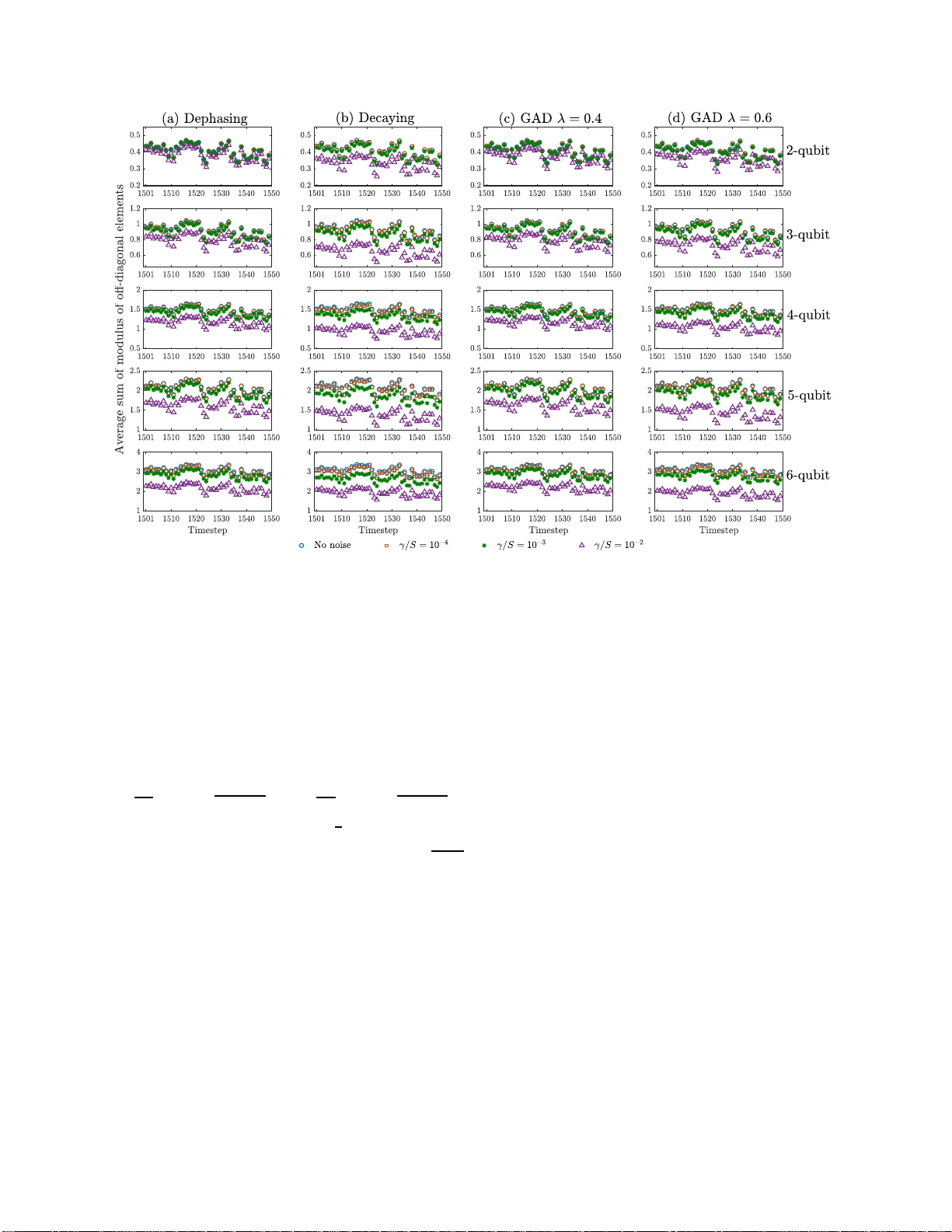
Learning Nonlinear Input-Output Maps with Dissipativ e Quan tum Systems Jia yin Chen and Hendra I. Nurdin ∗ Scho ol of Ele ctric a l Engine e ri n g and T ele c ommunic ations, The University of New South Wales (UNSW), Sydney NSW 2052, A ustr alia Abstract In this pap er, w e dev elop a theory of learning nonlinear inpu t-output maps with fading memory b y dissipativ e quant um systems, as a quan tum coun terp art of the theory of a pproximati ng such maps using cla ssical dyn amical systems. Th e theory ident iﬁes the pr op erties required for a class of dissipativ e quan tum systems to be universal , in that any input-output map w ith fading memory can b e appr o xim ated arbitrarily closely by an elemen t of this class. W e th en int ro du ce an example class of dissipativ e quan tum systems that is pro v ably u niv ersal. Num er ical exp er im ents ill ustrate that with a small n umber of qu b its, this class can ac h iev e co mparable p erforman ce to classical learning sc h emes with a large n umb er of tunable parameters. F urther numerical analysis suggests that the exp onen tially increasing Hilb ert space present s a p oten tial resource for dissipativ e quant um systems to surp ass classical lea rning sc hemes for inpu t-output maps. ∗ h.n urdin@unsw.edu.a u (cor resp onding a uthor) 1 I. INTR ODUCTIO N W e are in the midst of t he noisy interme diate-scale quan tum (NISQ) tec hnology era [39], mark ed b y noisy quantum computers consisting of roughly tens to h undreds of qubits. Curren tly there is a s ubstan tial in terest in early applications of thes e mac hines that can a c- celerate the dev elopmen t o f practical quan tum computers, akin to ho w the h umble hearing aid stim ulated the dev elopment of integrated circuit (IC) technology [30]. NISQ quan tum computing mac hines will not be equipp ed with quan tum error correction and are th us inca- pable of p erforming con tinuous q uan tum computation. Sev eral researc h directions are b eing explored f o r NISQ-class mac hines. One direction is to demonstrate so-called “quan tum supremacy”, in whic h NISQ ma chines can p erfo r m computational ta sks tha t are demonstrably out of the reac h of the most p o w erful digital sup ercomputers. The computationa l tasks include sampling problems suc h as b oson sam- pling [2, 27], instan taneous quan tum p olynomial (IQP) computation [11, 27], and sampling from random quan tum circuits [8]. Recen t w o r ks ha v e also prop osed quantum mac hine learning algorithms that oﬀer prov able sp eedups ov er their classical coun terparts [7 ]. An- other direction is the deve lopmen t of v ariat io nal algor it hms on h ybrid classical-quan tum mac hines to solv e certain classes of o ptimization problems. Algorithms prop osed include the quan tum appro ximate o ptimization algo r ithm (QA O A) [15], the quan tum v ariational eigensolv er (QVE) [29, 38] and v ariatio ns and generalizations thereof, e.g., [31, 47]. Exper- imen tal demonstration of QVE for calculating the ground-state energy of small molecules has b een rep orted in [22], while the a pplicatio n of QAO A for unsup ervised learning of a clustering problem can b e found in [35]. An alternativ e paradigm to the quan tum gate-based approac hes ab ov e is to harness the computational capabilit y of dissipativ e quantum systems. Dissipativ e quan tum dynamics has been sho wn to b e a ble to realize univ ersal quan tum computation [46] and has b een ap- plied in a time-delay fashion fo r sup ervised quantum machin e learning without in termediate measuremen ts [4]. Recen tly , quantum reserv oir computers (QR Cs) are intro duced to harness the complex real-time quan tum dissipativ e dynamics [17 , 32]. This approac h is essen tially a quan tum implemen t a tion of classical r e servoir c omputing sc hemes, in which a dynamical system pro cesses an input sequence and pro duces an output sequence that appro ximates a target sequence, see, e.g., [21, 26, 28]. The main philosoph y in r eserv oir computing is that the dynamics in arbitra r y naturally o ccurring or engineered dynamical systems could p oten- tially b e exploited for computational purp oses. In particular, a dynamical system could b e used for computat io n without precise tuning or optimization of it s parameters. T o possess temp oral information, the systems are required to satisfy three properties [28]: the c onver- genc e pr op erty [36], the fading memory pr op erty [10] and form a family of sys tems with the sep ar ation pr op erty . The con v ergence prop erty ensures that computations p erformed b y a dynamical system a re indep enden t of its initial condition, and t he fading memory prop erty implies that outputs of a dynamical system sta y close if the corresp onding inputs are close in recen t times. The separation prop erty states that there should b e a mem b er in the family of systems with dynamics suﬃcien tly rich to distinguish an y tw o diﬀerent input seque nces. Classical reserv oir computing has b een realized as simple nonlinear photonic circuits with a dela y line [5] a nd in neuromorphic computing based o n nanoscale oscillators [43], and it has b een demonstrated to achiev e state-of-the-art p erforma nce on applicatio ns suc h sp ok en digit recognition [43]. Nonlinear input-output (I/O) maps with fa ding memory can b e approx imated by a series 2 expansion suc h as the w ell-kno wn V olterra series [10]. They can also b e approx imated by a family of classic al nonlinear dynamical systems that ha ve the three pro p erties in tro duced in the previous paragraph. Suc h a fa mily of dynamical systems is said to b e universal (or p ossesses the univ ersality prop ert y) fo r nonlinear I/O maps with fading memory . They include v arious classical reserv o ir computing sc hemes suc h as liquid state mac hines [28], ec ho- state netw orks (ESNs) [18], linear reserv o ir s with p olynomial readouts (LR PO), and non-homogeneous state-aﬃne systems (SAS) [19]. Ho we v er, a theoretical framew ork for the learning of nonlinear fading memory I/O maps by quantum systems is so far lac king. Moreo v er, an extended inv estigation in to the p oten tial adv an tage quan tum systems oﬀer o v er classic al reserv oir computing sc hemes has not b een conducted. The pro vision of suc h a learning theory , the demonstration of a class of quantum mo del that is pro v ably univ ersal, and a study of this mo del via numerical exp erimen ts are the main con tributio ns of this pap er. The pap er is or g anized as follows . In Sec. I I, w e formally deﬁne fa ding memory maps. In Sec. I I I, w e fo r m ula te the theory o f learning no nlinear fading memory maps with dissipativ e quan tum systems. Sec. IV intro duces a concrete unive rsal class of dissipativ e quantum sys- tems. Sec. V num erically demonstrates the emulation p erformance o f the prop osed univ ersal class in the absence and presence of decoherence. The eﬀect of diﬀeren t input enco dings on the learning capability of this class is in v estigated. An in-depth comparison b et wee n this univ ersal class and ESNs is also conducted. W e conclude this section b y discussing the p otential of this univ ersal class to surpass classical sc hemes when implemen ted on a NISQ mac hine. In Sec. VI, w e discuss the f easibility of pro of- o f-principle exp erimen ts of the prop osed sch eme on existing NISQ mac hines. Detailed results a nd n umerical settings are collected in and can b e found in the App endix. I I. F ADING MEMOR Y MAPS Let Z denote the set of all in tegers and Z − = { . . . , − 1 , 0 } . Let u = { . . . , u − 1 , u 0 , u 1 , . . . } b e a real b ounded input sequence with sup k ∈ Z | u k | < ∞ . W e sa y that a real output sequence y = { . . . , y − 1 , y 0 , y 1 , . . . } is related to u by a time-inv ariant causal map M if y k = M ( u ) k = M ( ˜ u ℓ ) k for any integer ℓ , an y k ≤ ℓ , a nd an y sequ ence ˜ u ℓ suc h that ˜ u ℓ | ℓ = u | ℓ . Here, M ( u ) k denotes the output sequence at time k give n the input seque nce u , and u | k = { . . . , u k − 2 , u k − 1 , u k } is the input seq uence u truncated after time k . F or a ﬁxed real p ositiv e constant L and a compact subset D ⊆ R , w e a re in terested in the set K L ( D ) consisting of input sequences suc h that for all k ∈ Z , u k ∈ D ∩ [ − L, L ]. W e sa y a time-in v ariant caus al map M deﬁned on K L ( D ) has the fading memory prop ert y with resp ect to a decreasing sequence w = { w k } k ≥ 0 , lim k →∞ w k = 0 if, fo r an y t w o input sequence s u and v , | M ( u ) 0 − M ( v ) 0 | → 0 whenev er sup k ∈ Z − | w − k ( u k − v k ) | → 0. In other w o r ds, if the elemen ts of t w o sequences a gree closely up to some recen t past b efore k = 0, then their output sequences will also be close at k = 0. I I I. LEARNING NONLI NEAR F ADING MEMOR Y MAPS WIT H DISSIP A TIVE QUANTUM SYSTEMS Since fading memory maps are time-in v arian t, a n y dynamical system that is used to appro ximate them mus t forget its initial condition. Classical dynamical systems with this 3 prop erty are referred to a s c onver gent systems in control theory [36], and the prop ert y is kno wn as the e cho state pr op erty in the con text of ESNs [12, 21]. F or dissipativ e quan t um systems , this means that for the same input sequence, densit y o p erators asymptotically con v erge to the same sequence of densit y op erator s, indep enden tly o f their initial v alues. W e emphasize that the dissipativ e nature of the quan tum system is essen tial for the learning task. Without it the system clearly cannot be con v ergent. Consider a quantum system consisting of n qubits with a Hilb ert space C 2 n of dimension 2 n undergoing the follo wing discrete-time dissipativ e ev olution: ρ k = T ( u k ) ρ k − 1 , (1) for k = 1 , 2 , . . . , with initial condition ρ (0) = ρ 0 . Here, ρ k = ρ ( k τ ) is the system densit y op erator at time t = k τ and τ is a (ﬁxed) sampling time, and T ( u k ) is a completely p o sitiv e trace preserving (CPTP) map for eac h u k . In this setting, the real input sequence { u 1 , u 2 , . . . } determines the system’s ev olution. The o v erall input-output map in the long time limit is in general non-linear. Let k · k p denote an y Sc hatten p -norm for p ∈ [1 , ∞ ) deﬁned as k A k p = T r( √ A ∗ A p ) 1 /p , where A is a complex matrix and ∗ is the conjugate transp ose op erator. In App endix [VI I I A, Theorem 3] , w e sho w that if for all u k ∈ D ∩ [ − L, L ], the CPTP map T ( u k ) restricted on the h yp erplane H 0 (2 n ) of 2 n × 2 n traceless Hermitian op erators satisﬁes k T ( u k ) | H 0 (2 n ) k 2 − 2 : = sup A ∈ H 0 (2 n ) ,A 6 =0 k T ( u k ) A k 2 k A k 2 ≤ 1 − ǫ for some 0 < ǫ ≤ 1, then under an y input sequence u ∈ K L ( D ), it will forget its initial conditio n and is therefore con v ergent. This means that f o r any tw o initial densit y op erators ρ j, 0 ( j = 1 , 2) and the corresp onding densit y op erators ρ j,k at time t = k τ , w e will ha ve tha t lim k →∞ k ρ 1 ,k − ρ 2 ,k k 2 = lim k →∞      ← − Y k j =1 T ( u j )  ( ρ 1 , 0 − ρ 2 , 0 )     2 = 0 , where ← − Q k j =1 is a time-ordered comp osition of maps T ( u j ) from rig h t t o left. Let D ( C 2 n ) denote the conv ex set of all density o p erators on C 2 n . W e intro duce an o utput sequence ¯ y in the form ¯ y k = h ( ρ k ) , (2) where h : D ( C 2 n ) → R is a real functional o f ρ k . Eqs. (1) and (2) deﬁne a q uan tum dynam- ical system with input sequence u and output sequence ¯ y . W e now r equire the separation prop erty . Consider a family F of distinct quan tum systems described b y Eqs. (1) and (2), but p ossibly ha ving diﬀering num b er o f qubits. Let u and u ′ b e t w o input sequences in K L ( D ) that are not identic al, u k 6 = u ′ k for at least one k , and le t ¯ y and ¯ y ′ b e the respectiv e outputs of the quan tum system fo r these inputs. W e sa y that the family F is sep ar ating if for a ny non-iden tical inputs u a nd u ′ in K L ( D ), there exists a mem b er in this family with non-iden tical o utputs ¯ y and ¯ y ′ . As stated in App endix [VI I I B, Theorem 9], a n y family of con v ergen t dissipativ e quan tum systems that implemen t fading memory maps with t he separation prop ert y , a nd whic h forms an a lgebra of maps containing the constant maps, is univ ersal and can appro ximate an y I/O map with fading memory arbitrar ily closely . IV. A UNIVERSAL CLASS OF DISSIP A TIVE QUANTUM SYSTEMS W e no w specify a class of dissipativ e quan tum systems that is pro v ably univ ersal in appro ximating fading memory maps deﬁned on K 1 ([0 , 1 ]). The class consists of systems 4 that are made up o f N no n-inter acting subsystems initialized in a pro duct state of the N subsyste ms, with subsyste m K consisting of n K + 1 qubits, n K “system” qubits and a single “ancilla” qubit. W e la b el the qubits of subsystem K b y an index i K j that runs from j = 0 to j = n K , w ith i K 0 lab eling the a ncilla qubit. The n K + 1 qu bits in teract via the Hamiltonian H K = n K X j 1 =0 n K X j 2 = j 1 +1 J j 1 ,j 2 K ( X ( i K j 1 ) X ( i K j 2 ) + Y ( i K j 1 ) Y ( i K j 2 ) ) + n K X j =0 αZ ( i K j ) , where J j 1 ,j 2 K and α are real-v alued constants , while X ( i K j ) , Y ( i K j ) and Z ( i K j ) are P auli X , Y and Z op erat o rs of qubit i K j . The ancilla qubits for all subsy stems are p erio dically reset at time t = k τ and prepared in the input- dep enden t mixed state ρ K i 0 ,k = u k | 0 ih 0 | + (1 − u k ) | 1 ih 1 | (with 0 ≤ u k ≤ 1 ). The system qubits are initia lized at time t = 0 to some densit y op era t o r. The densit y op era t or ρ K k of the K th subsyste m qubits ev olv es during time ( k − 1) τ < t < k τ according to ρ K k = T K ( u k ) ρ K k − 1 , where T K ( u k ) is the CPTP map deﬁned by T K ( u k ) ρ K k − 1 = T r i K 0  e − iH K τ ρ K k − 1 ⊗ ρ K i 0 ,k e iH K τ  and T r i K 0 denotes the partial tr a ce o v er the a ncilla qubit of subsyste m K . W e no w specify an output functional h asso ciated with this sy stem. W e will use a single index to lab el the system qubits from t he N subsystems, the ancilla q ubits are not used in the output. Consider an individual system qubit with index j , with j running from 1 until n = P N K =1 n K . The output functional h is deﬁned to b e of the general form, ¯ y k = h ( ρ k ) = C + R X d =1 n X i 1 =1 n X i 2 = i 1 +1 · · · n X i n = i n − 1 +1 X r i 1 + ··· + r i n = d w r i 1 ,...,r i n i 1 ,...,i n h Z ( i 1 ) i r i 1 k · · · h Z ( i n ) i r i n k (3) where C is a constan t, R is an integer and h Z ( i ) i k = T r( ρ k Z ( i ) ) is the exp ectatio n of the op erator Z ( i ) . W e note that the f unctional h (the righ t hand side of the ab ov e) is a m ultiv ari- ate p olynomial in the v ariables h Z ( i ) i k ( i = 1 , . . . , n ) and these exp ectation v alues dep end on input sequence u = { u k } . Th us computing ¯ y k only in v olves estimating the exp ectations h Z ( i ) i k and the degree of the p olynomial R can b e c hosen as desired. If R = 1 then ¯ y k is a simple linear function of the expectations. This family of dissipativ e quantum systems exhibits tw o imp ortant prop erties, see Ap- p endix VI I I C and VI I I D for the pro ofs. F irstly , if for eac h subsyste m K with n K qubits and for all u k ∈ [0 , 1], k T K ( u k ) | H 0 (2 n K ) k 2 − 2 ≤ 1 − ǫ K for some 0 < ǫ K ≤ 1 , then this family forms a p olynomial algebra consis ting of systems that implemen t f ading memory maps. Secondly , a con v ergent single-qubit system with a linear output com binat io n of exp ectation v a lues (ie. n = 1, N = 1 and R = 1), separates p oin ts of K 1 ([0 , 1 ]). These tw o prop erties and a n application of the Stone-W eierstrass Theorem [13, Theorem 7.3.1 ] guarante e the univ ersalit y prop erty . The class sp eciﬁed ab ov e is a v ariant of the QR C mo del in [17] but is prov ably unive rsal b y the theory of the previous section. The diﬀerences are in the general form of t he output and, in our mo del, the a ncilla qubit is not used in computing the output. Also, w e do not consider time-m ultiplexing. W e remark that time-m ult iplexing can b e in principle incorp orated in the mo del using the same theory . Ho w ev er, this extension is more tec hnical and will b e pursued elsew here. 5 V. NUMERICAL EXPERIMEN TS W e demonstrate the em ulatio n p erformance of the univ ersal class in t ro duced ab o v e in learning a n um b er of b enc hmarking tasks. A ra ndom input sequence u ( r ) = { u ( r ) k } k > 0 , where eac h u ( r ) k is randomly uniformly chosen fr o m [0 , 0 . 2], is applied to all computational tasks. W e apply the m ultitasking me tho d, in whic h we sim ulate the ev olution of the quantum systems and record the exp ectations h Z ( i ) i k for all timesteps k once, while the output weigh ts C and w r i 1 ,...,r i n i 1 ,...,i n in Eq. (3) are optimized indep enden tly for eac h computational task. The linear reserv oirs with p olynomial outputs (LRPO) implemen t a fading memory map, whose discrete -time dynamics is of the form [10, 19], ( x k = Ax k − 1 + cu k y k = ˆ h ( x k ) , where w e c ho ose c ∈ R 1400 with elemen ts ra ndo mly unifo r mly chose n from [0 , 4] a nd ˆ h to b e a degree tw o m ultiv ar iate p olynomial, whose co eﬃcien ts are randomly uniformly c hosen from [ − 0 . 1 , 0 . 1]. W e c ho ose A to b e a diagonal blo c k matrix A = diag ( A 1 , A 2 , A 3 ), where A 1 , A 2 and A 3 are 200 × 200, 5 00 × 500 and 700 × 700 real matrices, respectiv ely . Elemen ts of A i ( i = 1 , 2 , 3) are randomly unifo r mly c hosen f r om [0 , 4]. T o ensure t he conv ergence and the fading memory prop ert y , the maxim um singular v alue of e ac h A i is randomly uniformly set to b e σ max ( A i ) < 1 [1 9]. In this setting, eac h linear reserv oir deﬁned by A i ev olves indep enden tly , while the out put of the LRPO dep ends on all state ele men t s x k ∈ R 1400 . It is intere sting to in v estigate the p erformance of the univ ersal class in learning t a sks that do not strictly implemen t fading memory maps as deﬁned here. W e apply the univ ersal class to approxim ate the outputs of a missile moving with a constan t v elo cit y in the horizontal plane [33] and the nonlinear autoregressiv e mo ving av erage (NARMA) mo dels [6]. The nonlinear dynamics of the missile is g iv en by ( ˙ x 1 = x 2 − 0 . 1 cos( x 1 )(5 x 1 − 4 x 3 1 + x 5 1 ) − 0 . 5 cos( x 1 ) ˜ u ˙ x 2 = − 65 x 1 + 5 0 x 3 1 − 15 x 5 1 − x 2 − 100 ˜ u where y = x 2 is the output. W e mak e a c hange of v aria ble of the input ˜ u = 5 u − 0 . 5 so that t he input range is the same as in [33]. The missile dynamics is sim ula ted b y the Runge-Kutta (4 , 5) form ula implemen ted by the o de45 function in MA TLAB [1 4], with a sampling time o f 4 × 10 − 4 seconds for a time span of 1 second, sub ject to the initial condition  x 1 x 2  T =  0 0  T . W e denote this task as Missile. The NARMA mo dels a r e often used to b enc hmark algorithms for learning t ime-series. The o utputs of eac h NARMA mo del dep end on its time-lagged outputs and inputs, speciﬁed by a dela y τ NARMA . W e denote t he corresp onding task to b e NARMA τ NARMA . W e fo cus on me m b ers of the unive rsal class with a single subsystem ( N = 1) and a small n um b er of system qubits n = { 2 , 3 , 4 , 5 , 6 } , and denote this subset of the univ ersal class as SA. W e will drop the subsystem index K from now on. F or all n umerical exp eriments , the parameters o f SA are chose n as follow s. W e in tro duce a scale S > 0 suc h that the Hamiltonian parameters J j 1 ,j 2 /S , α /S = 0 . 5 and τ S = 1 are dimensionless . As for t he Q RCs in [17], w e randomly uniformly generate J j 1 ,j 2 /S from [ − 1 , 1] and, to ensure conv ergence, select the resulting Ha milto nians f or exp erimen ts if the asso ciated CPTP map is conv ergen t. W e n umerically test the conv ergence prop erty b y chec king if 50 randomly generated initial 6 densit y op erators con v erge t o the same densit y op erato r in 500 timesteps under the input sequence u ( r ) . Eac h numerical experimen t ﬁrstly w ashouts the eﬀect of initia l conditions of SA and all target maps with 500 timesteps. This is follo w ed b y a training stage of 100 0 timesteps, where w e optimize the output weigh ts C a nd w r i 1 ,...,r i n i 1 ,...,i n of SA b y standard least squares to minimize the error P 1500 k =501 | y k − ¯ y k | 2 b et w een the t a rget output sequence y . In practical impleme n ta- tion, computation of the exp ectations h Z ( j ) i k is oﬄoaded to the quan tum subsystem, and only a simple classical pro cessing metho d is needed to o ptimize the output weigh ts. F or t his reason, w e asso ciate the output w eights C and w r i 1 ,...,r i n i 1 ,...,i n in Eq. (3 ) with (classic al) c omputa- tional no des , with the n um b er of suc h no des b eing equal to the num b er of output weigh ts. While the n umber of computationa l no des fo r SA can b e ch osen arbitrarily by v arying the degree R in the output, the state- space ‘size’ of the quantum system is 2 n (2 n + 1) − 2 n = 4 n . This state-space size corresp onds to the num b er of real v ariables needed to describ e the ev olutio n of elemen ts of the system densit y op erator. Note that since the densit y op erator has unit y trace, only up to at most 4 n − 1 of these no des are linearly indep enden t. On the other ha nd, for ESNs [21], the n um b er of computational no des a nd the state-space size alw a ys diﬀer b y one (i.e. b y the tunable constan t output w eight). F or an ESN with m reserv oir no des (E m ), the n um b er of computational no des is m + 1 and its state-space size is m . F or the V olterra series [10] with kerne l order o and memory p (V o, p ), the num b er of computational no des is ( p o +1 − p p − 1 + 1). W e select m and ( o , p ) suc h that t he num b er of computational no des is at most 801. This reduces the c hance of o v erﬁtting for learning a sequence of length 1 0 00 [25 ]. F or detailed n umerical settings for ESNs and the V olterra series, see App endix VI I I E. W e analyze t he p erformance of all learning sc hemes during an ev aluat io n phase consisting of 1000 timesteps , using the normalized mean-squared error NMSE : = P 2500 k =1501 | ¯ y k − y k | 2 / P 2500 k =1501 | y k − 1 1000 P 2500 k =1501 y k | 2 , where y is the target output and ¯ y is the approximated output. F or eac h task and e ac h n , NMSEs of 1 00 conv ergen t SA samples are a v eraged for analysis. A. Ov erview of SA learning p erformance W e presen t an ov erview of SA p erformance in learning the LR PO, Missile, NARMA15 and NARMA 20 tasks. The degree of the multiv ariate p olynomial output Eq . (3) is ﬁxed to b e R = 1 , so that the n um b er of computational is n + 1 for eac h n . Fig. 1 sho ws the t ypical SA o ut puts for the LRPO, Missile, NARMA 15 and NARMA20 tasks during the ev aluat io n phase. It is observ ed that the SA outputs follo w the LRPO outputs closely , while SA is able to approximate the Missile and NARMA tasks relativ ely closely . F or all computational tasks, as the n umber of system qubits n increases , the SA outputs b etter approximate the target outputs. This is quantitativ ely demonstrated in Fig. 2, whic h plo t s the a v erage SA NMSE as n increases. F rom Fig. 2 w e can see that the SA model with a small n um b er of computational no des p erforms comparably as ESNs and the V olterra series with a la rge num b er of computa- tional no des. F o r example, the av erage NMSE of 6-qubit SA with 7 computational no des is compar a ble to t he av erage NMSE o f E10 0 with 10 1 computational no des in the LRPO task. On av erage, 5-qubit SA with 6 computational no des p erforms b etter than V2 , 22 with 504 computational no des in the Missile task. In the NARMA15 t a sk, 4- qubit SA with 5 computational no des outp erfo rms V2 , 4 with 2 1 computational no des. In t he NARMA20 7 1501 1510 1520 1530 0 100 200 2001 2010 2020 2030 0 100 200 2471 2480 2490 2500 0 100 200 1501 1510 1520 1530 -0.05 0 0.05 0.1 2001 2010 2020 2030 -0.05 0 0.05 2471 2480 2490 2500 -0.02 0 0.02 0.04 1501 1510 1520 1530 0.15 0.2 0.25 2001 2010 2020 2030 0.15 0.2 0.25 2471 2480 2490 2500 0.15 0.2 0.25 1501 1510 1520 1530 0.2 0.25 0.3 2001 2010 2020 2030 0.2 0.25 0.3 2471 2480 2490 2500 0.2 0.25 0.3 FIG. 1. Typical SA outputs during the ev aluation phase, f or the (a) LRPO , (b) Missile (c) NARMA15 and (d) NARMA20 tasks. The leftmost, mid dle and righ tmost panels sho w the outputs for timesteps 1501-153 0, 2001-203 0 and 2471-250 0, resp ectiv ely task, 5-qubit SA performs comparably as E600. Our results are similar to the p erformance of the QRC s with time m ultiplexing rep orted in [17], where the QR Cs are demonstrated to p erform comparably as ESNs with a larger n um b er of trainable computatio na l nodes. Ho w- ev er, for the small n um b er of qubits in ve stigated, the rate o f dec rease in the av erage NMSE is a ppro ximately linear despite the dimension of the Hilb ert space increases exp onen tially as n increases. F or b oth the NARMA t a sks, the av erage NMSEs for 2-qubit and 6-qubit SA are of the same order of mag nitude. A larger n um b er of additional system qubits are required to substantially reduce the SA task error. B. SA p erformance under decoherence W e further v alidate the feasibilit y of t he SA mo del in the presence of the dephasing, deca ying noise and the generalized amplitude damping (GAD) c hannel. W e simu late the noise by a pplying the T rotter-Suzuki form ula [4 2, 44 ], in whic h we divide the normalized time inte rv al τ S = 1 into 50 small time in terv als δ t = τ S/ 50, and alternativ ely apply the unitary in teraction and the Kraus op erators { M ( j ) l ( γ S ) } l of eac h noise t yp e, each for a time duration of δ t . Each of the l -th Kraus op erator is applied fo r all system and a ncilla qubits j = 1 , . . . , n + 1, and γ /S denotes the noise strength. F or all noise t yp es, w e apply the same noise strengths γ /S = { 10 − 4 , 10 − 3 , 10 − 2 } , whic h are within the exp erimen ta lly f easible range for systems lik e NMR ensem bles [4 5] and some curre n t sup erconducting NISQ machine s [1]. Under the dephasing noise, the densit y op erator ρ of the system and ancilla qubits ev o lv es 8 FIG. 2. Av erage S A NMSE for the (a) LRPO, (b) Missile, (c) NARMA15 and (d) NARMA20 tasks, th e err or bars rep r esen t the standard error. F or comparison, horizont al dashed lines lab eled with “E m ” ind icate the a v er age p erformance of ES Ns with m computational n o des, and horizon tal dot-dashed lines lab eled with “V o, p ” indicates the p erformance of V olterra series with k ernel order o and memory p . Overlapping d ash ed and dot-dashed lines are represen ted as dashed lines according to ρ → 1+ e − 2 γ S δ t 2 ρ + 1 − e − 2 γ S δ t 2 Z ( j ) ρZ ( j ) , suc h that the diagonal elemen ts in ρ remain in v arian t while t he o ﬀ-diagonal elemen t s decay . The GAD c hannel giv es rise to the ev olution ρ → P 3 l =0 M ( j ) l ( γ S , λ ) ρ ( M ( j ) l ( γ S , λ )) † , where † denotes the a dj o in t, and the Kraus op erators M ( j ) l ( γ S , λ ) ( l = 0 , 1 , 2 , 3) dep end on an additional ﬁnite temp erature parameter λ ∈ [0 , 1] [34]. When λ = 1, w e recov er the amplitude damping c hannel (the deca ying no ise), whic h tak es a mixed state into the pure ground state | 0 ih 0 | in the long time limit. F or λ 6 = 1, w e in v estigate the SA task p erfo rmance under the GAD channel fo r λ = { 0 . 2 , 0 . 4 , 0 . 6 , 0 . 8 } . The GAD c hannel aﬀects b oth the diago nal and oﬀ- diagonal elemen ts of the dens it y op erator. Fig. 3 plots the av erage SA NMSE under the dephasing, decaying a nd GAD with λ = { 0 . 4 , 0 . 6 } for all no ise strengths. See App endix VI I I E 2 for the av erage NMSE under the GAD channel for all c hosen temp erature parameters. Fig. 3 indicates that for the same noise strength, diﬀeren t noise t yp es a ﬀ ect the SA t ask p erformance in a similar manner. F or noise strengths γ /S = { 10 − 4 , 10 − 3 } , all noise types do no t signiﬁcan tly degrade SA task p erformance for t he computatio nal tasks. Ho w ev er, the impact of the noise strength γ /S = 10 − 2 is more prono unced, particularly for a larger n umber of system qubits. Changes in the SA task error under the eﬀect of the deca ying noise and the G AD c hannel are an ticipated, since the exp ectations h Z ( j ) i k in the output dep end on the diagonal elemen ts of the system densit y op erator, whic h are a ﬀected b y b oth of these noise types. How ev er, the SA task p erforma nce is also aﬀected b y the dephasing no ise, which do es not c hange the diagonal elemen ts. A p ossible explanation f or this b eha vior is a lo ss of degrees o f freedom, in the sense that oﬀ- diagonal elemen ts o f the densit y op erator b ecome smaller and the densit y op erator lo o ks more lik e a classical probability distribution. Alternativ ely , this could b e view ed as the oﬀ-diagonal elemen ts con tributing less to the ov erall computation. T o supp o rt this explanation, for the dephasing, decay ing and the GAD with λ = { 0 . 4 , 0 . 6 } , and for eac h n , we sum the complex mo dulus of o ﬀ - diagonal elemen ts in the system densit y op erator fo r the 100 n -qubit SA samples sim ulated abov e. The av erage o f these 100 sums is plotted for the ﬁrst 50 time steps during the ev aluatio n phase in Fig. 4. That is, Fig. 4 plots 2 n s P n s l =1 P 2 n r =1 P 2 n s = r +1 | ρ ( l ) k ,r s | , where n s = 100 is the n um b er of diﬀeren t random SA samples. 9 FIG. 3. Ave rage S A NMSE for the LRP O, Missile, NARMA15 and NARMA2 0 tasks under d eco- herence. F or comparison, the a v erage SA NMSE without the eﬀect o f noise is also plotted. In all plots, the err or bars represent the standard error Here ρ ( l ) k ,r s denotes the elemen t of ρ ( l ) k in ro w r a nd column s (the sup erscript ( l ) indexing the SA sample). Fig. 4 s how s that as the noise strength increases, the av erage sum decreases, particularly with the noise strength γ /S = 10 − 2 . Similar trends are o bserv ed fo r the GAD c ha nnel for all the temp erature parameters c hosen, and the observ ed trend for the av erage sum p ersists as t he timestep increases t o 2 5 00 (see App endix VI I I E 2). The results presen ted in Fig. 4 further indicate that though the o utput of SA dep ends solely on the diagonal elemen ts of t he densit y op erator, nonzero oﬀ-diagonal elemen ts are crucial for impro ving the SA em ulation p erformance. This pro vides a plausible explanation for the improv ed p erformance ac hiev ed b y increasing the n um b er of qubits, thereb y increasing Hilb ert space size and the n um b er of non-zero oﬀ-diag o nal elemen ts. F urther inv estigation in to this topic is presen ted in Sec. V D . 10 FIG. 4. Ave rage sum of complex modu lus of oﬀ-diagonal elemen ts in the system den sit y op erator for timesteps 1501-155 0, under the (a) deph asing noise, (b) deca ying n oise, (c) GAD with λ = 0 . 4 and (d) GAD with λ = 0 . 6. Ro w n − 1 in the ﬁgure corresp ond s to the a ve rage su m for n -qubit SA C. Eﬀect of diﬀere nt input encodings Our pro p osed univ ersal class enco des the input u k ∈ [0 , 1] into the mixed state ρ i 0 ,k = u k | 0 ih 0 | + (1 − u k ) | 1 ih 1 | . Ot her input enco ding p ossibilities include the pure state ρ i 0 ,k = ( √ u k | 0 i + √ 1 − u k | 1 i )( √ u k h 0 | + √ 1 − u k h 1 | ) used in the QR C mo del [17], enco ding the input in to the phase ρ i 0 ,k = 1 2 ( | 0 i + e − iu k | 1 i )( h 0 | + e iu k h 1 | ), and enco ding the input in to non- orthogonal basis state ρ i 0 ,k = u k | 0 ih 0 | + 1 − u k 2 ( | 0 i + | 1 i )( h 0 | + h 1 | ). W e denote these diﬀeren t input encodings as mixed, pure, phase and non-orthogona l. W e emphasize that for the last three enco dings the univ ersalit y of the asso ciated dissipativ e quan tum system using these enco dings has not b een prov en. T o in v estigate the impact of input enco dings on the computational capability of quan tum systems , t he Hamilto nia n parameters for all quan tum systems sim ulated here are sampled from the same unifo rm distribution, and the resulting Hamiltonia ns a r e chosen if the as- so ciated CPTP map tha t implemen ts the sp eciﬁed input-dep enden t densit y op erator ρ i 0 ,k is conv ergen t. W e again test the conv ergence prop ert y numerically b y chec king if 50 ran- domly generated initial density o p erators conv erge to the same densit y op erator within 500 timesteps. The n um b er of system qubits and the num b er of computational no des fo r all input enco dings are the same. F or eac h input enco ding, NMSEs of 100 con v ergent quan- tum systems are a v era g ed for analysis. Fig. 5 sho ws that for all computational ta sks, the mixed state enco ding p erfo rms b etter t ha n other enco dings. H ow ev er, the av erage NMSE 11 for diﬀeren t input enco dings fo r all computational ta sks a re of the same order of magnitude. Moreo v er, as the num b er of sy stem qubits increases, the errors of diﬀe ren t input enco dings decrease at roughly the same rate. This comparison indicates that the eﬀect of diﬀeren t input encodings on the learning p erformance do es not a pp ear signiﬁc an t. 2 3 4 5 6 0 0.1 0.2 0.3 0.4 0.5 0.6 0.7 0.8 2 3 4 5 6 0.1 0.2 0.3 0.4 0.5 0.6 0.7 0.8 0.9 2 3 4 5 6 0.5 0.55 0.6 0.65 0.7 0.75 0.8 0.85 2 3 4 5 6 0.5 0.55 0.6 0.65 0.7 0.75 0.8 0.85 0.9 FIG. 5. Av erage NMSE for diﬀerent input enco dings, f or approxima ting the (a) LRPO, (b) Missile (c) NARMA15 and (d) NARMA 20 tasks. Er ror b ars represent the standard error D. F urther comparison wit h ESNs Our nume rical results so far and the results sho wn in [17 ] b oth suggest tha t dissipativ e quan tum systems with a small n umber of qubits ac hiev e comparable p erformance to classical learning sc hemes with a large n um b er of computationa l nodes. Ho w ev er, these comparisons ma y app ear to b e sk ew ed fa v orably tow ard quantum dynamical systems, since it do es not address their exp onen t ia l state-space size. One can, for example, also increase the state- space size of ESNs a nd the num b er of computational no des of SA, suc h that the state-space size and the num b er of computational no des are similar for both mo dels. Here we pr esen t a further comparison bet w een the SA mo del and ESNs, and pro vide insigh ts into the p ossible adv an tage the SA mo del migh t oﬀer o v er its classical coun terpart. W e fo cus on 4 - qubit SA with a state-space size of 256. Setting R = 6 in Eq. (3), the n um b er of computational no des for SA is 21 0. W e compare t his 4- qubit SA mo del’s av erage task p erformance with the av erage E256 task p erformance in appro ximating the LRPO, Missile, NARMA15, NARMA20, NARMA30 and NARMA40 tasks. Here, the n um b er of computational no des for E256 is 257 and the av erage NMSE of 100 con v ergen t E256s is rep orted. As sho wn in T able 1, f o r the Missile and all the NARMA tasks, the av erage NMSEs for b oth mo dels are of the same order of magnitude, while E256 outp erforms SA in the LR PO task. This comparison suggests that when the state-space size and the num b er of computational nodes for both mo dels are similar, ESNs can outp erfor m the SA mo del. W e further inv estigate under what conditions SA migh t o ﬀer a computational adv an- tage. W e observ e t ha t while t he n um b er of computational no des is ke pt constant, increasing the state-space size of SA induces a considerable computational improv emen t. T o demon- strate this, 4- , 5- and 6-qubit SA samples are sim ulated to perf o rm all computationa l tasks men tioned ab o v e. F or each n -qubit SA, we v ary its o utput degree R suc h that its n um- b er of computational no des ranges from 5 to 25 2 . The chose n degrees for 4-qubit SA a re R 4 = { 1 , . . . , 6 } , for 5- qubit are R 5 = { 1 , . . . , 5 } , and f or 6-qubit SA a re R 6 = { 1 , . . . , 4 } . 12 T ABLE 1. Averag e 4-qubit SA and E256 NMSE f or the LRPO , Missile, NARMA15, NARMA20, NARMA30 and NARMA40 tasks. Results are roun ded to t w o signiﬁcant ﬁ gures. The notation ( ± se) denotes the stand ard error T ask SA NMSE ( ± se) E256 NMSE ( ± se) LRPO 0 . 20 ± 1 . 5 × 10 − 2 0 . 019 ± 7 . 7 × 10 − 4 Missile 0 . 48 ± 2 . 2 × 10 − 2 0 . 49 ± 3 . 3 × 10 − 3 NARMA15 0 . 61 ± 8 . 0 × 10 − 3 0 . 32 ± 1 . 6 × 10 − 4 NARMA20 0 . 68 ± 1 . 0 × 10 − 2 0 . 67 ± 3 . 2 × 10 − 4 NARMA30 0 . 67 ± 7 . 1 × 10 − 3 0 . 67 ± 4 . 0 × 10 − 4 NARMA40 0 . 64 ± 5 . 3 × 10 − 3 0 . 66 ± 5 . 9 × 10 − 4 F or eac h n -qubit SA, the Hamiltonians are the same for all its chosen output degrees, and the task errors of 100 con v ergen t SA samples are a v eraged for analysis. F or comparison, w e sim ulate 100 con v ergent ESNs with reserv oir size 256 to p erform the same ta sks. F or n -qubit SA, let N n ( n = 4 , 5 , 6) denote the n um b ers of computatio nal no des corresp onding to its output degrees R n . The n um b er of computational no des C f or E256 is set to b e elemen ts in the set N 4 ∪ N 5 ∪ N 6 . W e ﬁrst optimize 257 output w eigh ts for E256 via standard least squares during the training phase. When C < 257 for E256, we select C − 1 computational nodes (excluding the tunable constan t computat io nal node) with the largest absolute v a lues and their corresp onding state elemen ts. These C − 1 state elemen t s ar e used to re-o pt imize C computational nodes (including the tunable constan t c omputational node) via standard least squares. During the ev aluation phase, 2 56 state elemen ts ev olv e; only C − 1 state elemen ts and C output w eigh ts are used to compute the E256 output. Fig. 6 plots the 4- , 5-, and 6- qubit SA av erage NMSE as the n um b er of computational no des increases for all computationa l tasks. F or comparison, the a v era g e E256 NMSE is also plotted. Tw o imp ortan t observ a tions are that increasing the num b er of computational no des do es not necessarily improv e SA task p erformance, while increasing the state-space size induces a noticeable impro v emen t. F o r example, for the NARMA20 ta sk and 210 computational no des, the av erage NMSE for 4-qubit SA is 0.68 while the av erage NMSE for 6-qubit SA is 0.48 . When comparing to E256 , we observ e that fo r most tasks, despite 4-qubit SA might not p erform b etter than E256 , subsequen t increases in the state-space size a llo w t he SA mo del to outp erform E256, without extensiv ely increasing its n um b er of computational no des. Con t r a ry to the ab ov e observ ations fo r the SA mo del, increasing the reserv oir size of ESNs while ke eping the n um b er of computational no des ﬁxed do es not induce a signiﬁcan t compu- tational improv emen t. T o nu merically demonstrate this, the reserv oir size of ESNs is further increased to { 300, 400, 50 0 } . F or e ac h reserv oir size, the num b er of computational no des is set to b e the same as that of E256. These computational no des are chose n and optimized by the same metho d describ ed a b o v e for E256. W e av erage the task errors of 10 0 conv ergen t ESNs for eac h reserv oir size. As sho wn in Fig. 7, noticeable p erformance improv emen ts fo r ESNs are only observ ed as the n um b er o f computational no des increases, but not as t he reserv oir size v aries. Another observ ation is that for the NARMA30 and NARMA40 tasks , the erro r increases as the num b er of computational no des f o r ESNs increases. This could b e due to o verﬁtting, a condition occurs when to o man y adjustable parameters are trained on limited training data [16]. O n the other hand, this obs erv ation is less signiﬁcan t for the SA 13 5 15 21 28 35 56 70 84 126 210 252 0 0.5 5 15 21 28 35 56 70 84 126 210 252 0 0.5 1 5 15 21 28 35 56 70 84 126 210 252 0.2 0.4 0.6 5 15 21 28 35 56 70 84 126 210 252 0.4 0.6 0.8 5 15 21 28 35 56 70 84 126 210 252 0.5 0.6 0.7 5 15 21 28 35 56 70 84 126 210 252 0.6 0.7 FIG. 6. Av erage SA NMSE as the state-space size and the n umber of computational no des v ary for all computational tasks. Th e a verage NMSE for E256 w ith the same num b er of computational no des is plotted for comparison. The d ata symbols obscu r e the error b ars, which r ep resen t the standard error mo del. It w ould b e in teresting to conduct further inv estigation in to this b ehav ior in future w o r k. The ab o v e o bserv at ions ha v e sev eral implications. T o impro v e the computational capa- bilit y of the SA mo del, one can tak e adv an tage of the exp onen tially increasing state-space size of the Hilb ert space while only optimizing a p olynomial num b er o f computational no des. On the con trary , to impro v e the computational capability of ESNs, o ne needs to increase the n um b er of computational no des, whic h is bounded b y the r eserv oir size. Therefore, enhanc - ing em ulation p erformance of ESNs inevitably req uires the state- space s ize to b e increased. In the situation where the state-space size increases b eyond what classical computers can sim ulate in a reasonable amount of time and with reasonable resources (such as memory), the computational capabilit y of ESNs saturates, whereas the computational capa bilit y of the SA mo del could b e fur t her impro v ed by increasing the n um b er of qubits in a linear fashion. In this regime, the SA mo del could prov ide a p o t ential computational adv antage o v er its classical coun terpart. T o furt her v erify the feasibility of this hy p othesis, the learn- ing capabilit y of the SA mo del would need to b e ev aluated fo r a larger n umber of qubits on a ph ysical quantum system. A p ossible implemen tatio n of this exp erimen t is on NMR ensem bles, as suggested in [17]. How ev er, motiv ated b y the av aila bilit y of NISQ mac hines, a quan tum circuit implemen tation of t he SA mo del, using the sc hemes prop osed in [9, 20], w o uld b e more att ractiv e. This is another topic of further researc h con tin uing from this w o r k. 14 FIG. 7. Ave rage ESNs NMSE as the state-space size and the num b er of computational n o des v ary for all computational tasks. The d ata symb ols obscure the error bars, which represent the standard error VI. DISCUSSION W e discuss the feasibility of realizing the prop osed unive rsal sc heme in Section IV on the curren t most scalable NISQ quan tum computers , suc h as quantum compute rs based o n sup erconducting circuits or io n traps. W e consider those that implemen t the quantum circuit mo del. Simulating the unitary in teraction giv en b y the Ising Hamiltonian H K on a quan tum circuit requires decomp o sition of the evolution using the T rotter-Suzuki pro duct fo r mula [42, 44]. Suc h a decomp osition may require the sequen tial application of a larg e num b er of g ates on NISQ ma chines , limiting the implemen tabilit y o f this fa mily o n curren t NISQ mac hines due to sev ere decoherence. Ho w ev er, it ma y b e p ossible to engineer alternativ e families based on simpler unitary in teractions b et w een the subsyste m and ancilla qubits (not of the Ising t yp e), using only a short sequenc e of single-qubit a nd t w o -qubit gates, suc h that the ass o ciated CPTP maps p ossess the con vergenc e and fading memory prop erties. A general framew ork for constructing suc h unitary in teractions is the sub ject of o n-going and future w ork con tin uing from this paper. T o realize the dis sipativ e dynamics for a subsys tem, we can construct a quan tum circuit as follo ws. At eac h t imestep k , the ancilla qubit is prepared as the input-dep enden t mixed state ρ K i 0 ,k . After the unitary in teraction with the subsystem qubits, the partial trace ov er 15 the ancilla qubit can b e p erformed by a pro jectiv e measuremen t on the ancilla qubit and discarding the measuremen t outcome. A t the next time step k + 1 , the ancilla qubit is reset and prepared as ρ K i 0 ,k +1 . T o estimate the exp ectations h Z ( j ) i k , w e p erform Mon te Carlo estimation b y running the circuit m ultiple times and measuring Z ( j ) at time k , the a v erage of measured results o v er these runs estimates h Z ( j ) i k . If multiple NISQ mac hines can b e run in pa rallel at the same time , the expectations h Z ( j ) i k can be estimated in real time. In this setting, the num b er of qubits required to implemen t a dissipativ e subsystem for temp oral learning is n K + 1 . Some exis ting NISQ mac hines based on superconducting circuits are not capable of preparing mixed states or resetting qubits for reuse aft er measuremen t. T o address the ﬁrst limitation, w e can appro ximate the ancilla input- dep enden t mixed state ρ K i 0 ,k b y Mon te Carlo sampling. That is, we construct M > 0 quan t um circuits as ab ov e, but f o r eac h circuit and at each timestep k , w e prepare the ancilla qubit in | 0 i with probability u k or in | 1 i with probabilit y 1 − u k . W e aga in remark tha t thes e M quan tum circuits can b e run in parallel, and therefore computations could b e p erformed in real time if m ultiple circuits can b e r un at the same time. Not being able to reuse a qubit after a measuremen t means that eac h point in the input sequence mu st b e enco ded in a distinct qubit. This implies that the length of sequence s t hat can b e considered will b e limited b y the n um b er of qubits a v ailable. Some of the qubits av ailable will need to b e a ssigned as the system qubits while a ll the other qubits as data carr ying ancilla qubits. F or instance, on a 20 -qubit mac hine, one can use sa y 4 qubits as the system q ubits and the remaining 16 qubits for carrying the input sequence. In this cas e the total input sequence length that can be pro cessed for w ashout, learning and ev aluation is only of length 1 6. Nev ertheless, curren t high-p erformance quan tum circuit sim ulators, suc h as the IBM Qiskit simulator (h ttps://qiskit.org/) [3], are capable of simu lating qubit reset and realistic hardw are noise. W e also antic ipate that the qubit reset functionality on NISQ machines would b e av ailable in the near future, op ening a v enue fo r pro of-of-pr inciple exp eriments of the prop osed sc heme fo r input sequences of arbitrary length. VI I. CO NCLUSION AND OUTLO OK W e hav e dev elop ed a general theory for learning arbitrary I/O ma ps with fading memory using dissipative quan tum systems. The a t t r activ eness of the theory studied here is that it allows a dissipativ e quan tum system (that meets certain requiremen ts but is otherwise arbitrary) to b e com bined with a classical pro cessor to learn I/O maps from sample I/O sequence s. W e apply the theory to demonstrate a univ ersal class of dissipativ e quan tum systems that can approx imate arbitrary I/O maps with fading memory . Numerical exp erimen ts indicate that eve n with only a small num b er of qubits and a sim- ple linear output, this class can ach iev e compara ble p erfor ma nce, in terms of the av erage normalized mean-squared error, to classical learning sc hemes such as ESNs and the V olterra series with a la r ge n um b er of tunable par a meters. Ho w ev er, when the stat e- space sizes of the quantum subsystem and classical lear ning sche mes are the same, and the nu m b er of computational no des equals the num b er of no des in the ESN plus one (for the constan t term) and a similar n um b er of the QR C, the quan tum system do es not demonstrate an y computational adv an tage. Moreov er, the n umerical results for a small n um b er of qubits in- dicate t ha t increasing the dimension of the Hilb ert space of the quan tum system while ﬁxing the n um b er of computationa l no des can still result in impro v ed prediction p erformance on a n um b er of b enc hmarking tasks, whereas increasing t he state space of ESNs while ﬁxing the 16 computational no des do es not lead to a ny noticeable impro v emen t. This strongly suggests that the p ossibly very large Hilb ert space of the quan t um subsystem presen ts a p ot ential resource that can be ex ploited in this approac h. That is, for state-space dimensions b ey ond what can b e sim ulated on a con ve n tional digital computer. It remains to b e in v estigated if this resource can indeed lead to a prov able p erformance adv an tage ov er con v entional classical learning approac hes, and the circumstance s where this will b e the case. VI I I. APP ENDIX A. The con v ergence prop ert y Recall from the main text that for a compact subset D ⊆ R and L > 0, K L ( D ) denotes the set of all real sequences u = { u k } k ∈ Z taking v alues in D ∩ [ − L, L ]. Let K − L ( D ) and K + L ( D ) b e subsets of input sequences in K L ( D ) whose indices a r e restricted to Z − = { . . . , − 2 , − 1 , 0 } and Z + = { 1 , 2 , . . . } , resp ectiv ely . In the follo wing, we write T for b oth input-indep enden t and input-dep enden t CPTP maps. As in the main text, w e write T ( u k ) for a CPTP map that is determined b y a n input u k , and k · k p for any Sc hatten p -norm fo r p ∈ [1 , ∞ ). All dissipativ e quantum systems considered here are ﬁnite-dimensional. W e now state the deﬁnition of a con v ergen t CPTP map with resp ect to K L ( D ). Deﬁnition 1 (Con v ergence) . A n in p ut-dep endent CPT P map T is c onver gent with r esp e ct to K L ( D ) if ther e exists a se quenc e δ = { δ k } k > 0 with lim k →∞ δ k = 0 , such that fo r al l u = { u k } k ∈ Z + ∈ K + L ( D ) and an y two density op er ators ρ j,k ( j = 1 , 2) satisfying ρ j,k = T ( u k ) ρ j,k − 1 , it hold s that k ρ 1 ,k − ρ 2 ,k k 2 ≤ δ k . We c al l a di s sip ative quantum system w hose dynamics is gov e rne d by a c onver g ent CPTP map a c onver gen t system. The conv ergence prop ert y can b e view ed as a n extension of the mixing prop erty for a noisy quan tum c hannel described b y an input-indep enden t CPTP map [40 ]. Deﬁnition 2 (Mixing) . A n -qubit dis s i p ative quantum system describ e d by a CPTP map T is mixi n g if for al l ρ 0 ∈ D ( C 2 n ) , if ther e exists a unique density op er ator ρ ∗ such that, lim k →∞      k Y j =1 T ( ρ 0 ) ! − ρ ∗      2 = 0 . W e will see later that if an input-dep enden t CPTP map T ( u k ) satisﬁes the suﬃcien t condition in T heorem 3, then T ( u k ) is mixing for eac h u k ∈ D ∩ [ − L, L ]. Theorem 3 (Conv ergence prop erty ) . A n -qubit dissip ative quantum system governe d by an input-dep end ent CPTP map T is c onver gent with r esp e ct to K L ( D ) if, for al l u k ∈ D ∩ [ − L, L ] , T ( u k ) on the hyp erplane H 0 (2 n ) of 2 n × 2 n tr ac eless Hermitian op er ators satisﬁes k T ( u k ) | H 0 (2 n ) k 2 − 2 : = sup A ∈ H 0 (2 n ) ,A 6 =0 k T ( u k ) A k 2 k A k 2 ≤ 1 − ǫ for some 0 < ǫ ≤ 1 . Mor e over, any p air of initial density op er ators c on ver ge uniformly to one another under T . Pr o of. Let ρ 1 , 0 and ρ 2 , 0 b e tw o arbitrary initial densit y op erators, ρ 1 , 0 − ρ 2 , 0 is a tr a celess 17 Hermitian op era t or. W e ha v e, k ρ 1 ,k − ρ 2 ,k k 2 =      ← − Y k j =1 T ( u j )  ( ρ 1 , 0 − ρ 2 , 0 )     2 =      ← − Y k j =1 T ( u j ) | H 0 (2 n )  ( ρ 1 , 0 − ρ 2 , 0 )     2 ≤ ← − Y k j =1   T ( u j ) | H 0 (2 n )   2 − 2 k ρ 1 , 0 − ρ 2 , 0 k 2 ≤ ← − Y k j =1 (1 − ǫ ) k ρ 1 , 0 − ρ 2 , 0 k 2 ≤ ← − Y k j =1 (1 − ǫ )( k ρ 1 , 0 k 2 + k ρ 2 , 0 k 2 ) ≤ 2 (1 − ǫ ) k , where the la st inequalit y follow s from the fa ct tha t for all ρ ∈ D ( C 2 n ), k ρ k 2 ≤ 1 . W e remark that f o r a n -qubit dissipativ e quan tum system that satisﬁes the condition in Theorem 3, an y initial density op erator ρ 0 reac hes the state lim k →∞  ← − Q k j =1 T ( u j )   I 2 n  . T o see this, let ρ 0 = I 2 n + X j 1 ,j 2 ,...,j n = { 0 , 1 , 2 , 3 } j 1 j 2 ...j n 6 =0 α j 1 j 2 ...j n n O i =1 σ ( i ) j i , where σ ( i ) j i denotes, for qubit i , t he identit y op erator I if j i = 0, the Pauli X op erator if j i = 1, the P auli Y op erator if j i = 2 a nd the P auli Z op erator if j i = 3. Since N n i =1 σ ( i ) j i for j 1 j 2 . . . j n 6 = 0 are all traceless Hermitian op erators, therefore as k → ∞ ,     ρ k −  ← − Y k j =1 T ( u j )   I 2 n      2 → 0 . B. The univ ersality property W e no w sho w the univ ersality prop erty of con v ergent dissipativ e quan tum system s. Let R Z b e the set of all real-v alued inﬁnite sequence s. Consider a n -qubit con v ergen t dissipativ e quan tum system describ ed by Eqs. (1) a nd (2) in the main text, whose dynamics and output are deﬁned by a CP TP map T and a functional h : D ( C 2 n ) → R , resp ectiv ely . W e associate this quan tum system with an induced ﬁlter M T h : K L ( D ) → R Z , suc h that for any initial condition ρ −∞ ∈ D ( C 2 n ), when ev aluated at time t = k τ , M T h ( u ) k = h  − → Y ∞ j =0 T ( u k − j )  ρ −∞  , where − → Q ∞ j =0 T ( u k − j ) = lim N →∞ ← − Q N j =0 T ( u k +( j − N ) ) = lim N →∞ T ( u k ) T ( u k − 1 ) · · · T ( u k − N ), and the limit is a po in t wise limit. Lemma 4 states that this limit is w ell-deﬁned. Lemma 4. The ﬁlter M T h : K L ( D ) → R Z is wel l-deﬁne d. In p articular, the limit lim N →∞ T ( u k ) T ( u k − 1 ) · · · T ( u k − N ) ρ − N exists and is indep enden t of ρ − N . 18 Pr o of. The set D ( C 2 n ) equipped with the distance function indu ced by the norm k · k 2 is a complete metric space. Therefore, ev ery Cauc h y sequence conv erges to a p oint in D ( C 2 n ) [41]. It remains to sho w t ha t S n = T ( u k ) T ( u k − 1 ) · · · T ( u k − n ) ρ − n is a Cauc h y sequence . By h yp othesis, fo r all u k ∈ D ∩ [ − L, L ], k T ( u k ) | H 0 (2 n ) k 2 ≤ 1 − ǫ for some 0 < ǫ ≤ 1 . F or a n y ǫ ′ > 0, let N > 0 suc h that (1 − ǫ ) N < ǫ ′ 2 . Then for a ll n, m > N , supp ose that n ≤ m , k S n − S m k 2 = k T ( u k ) T ( u k − 1 ) · · · T ( u k − n ) ( ρ − n − T ( u k − n − 1 ) · · · T ( u k − m ) ρ − m ) k 2 ≤ (1 − ǫ ) n +1 ( k ρ − n k 2 + k ( T ( u k − n − 1 ) · · · T ( u k − m )) ρ − m k 2 ) ≤ 2(1 − ǫ ) N < ǫ ′ This ﬁlter is causal since given u , v ∈ K L ( D ) satisfying u τ = v τ for τ ≤ k , M T h ( u ) k = M T h ( v ) k . F or an y τ ∈ Z , let M τ b e the shift op erator deﬁned b y M τ ( u ) k = u k − τ . A ﬁlter is said to be time-in v arian t if it comm utes with M τ . It is straigh tforw ard to sho w that M T h is time-in v arian t. F or a time-in v arian t and causal ﬁlter, there is a corresp o nding functional F T h : K − L ( D ) → R deﬁned a s F T h ( u ) = M T h ( u ) 0 (see [10]). The corresp onding ﬁlter can b e reco vered via M T h ( u ) k = F T h ( P ◦ M − k ( u )), where P truncates u up to 0 , that is P ( u ) = u | 0 . W e sa y a ﬁlter M T h has the fading memory pro p ert y if and only if F T h is contin uous with respect to a w eighted norm deﬁned as follo ws. Deﬁnition 5 (W eigh ted norm) . F o r a n ul l se quenc e w = { w k } k ≥ 0 , that is w : { 0 } ∪ Z + → (0 , 1 ] is de cr e asing and lim k →∞ w k = 0 , deﬁne a weighte d norm k · k w on K − L ( D ) as k u k w : = sup k ∈ Z − | u k | w − k . Deﬁnition 6 (F ading memory) . A time-invaria n t c ausal ﬁlter M : K L ( D ) → R Z has the fading memory pr op erty with r es p e ct to a nul l se quenc e w if and only if i ts c orr esp onding functional F : K − L ( D ) → R is c ontinuous with r esp e ct to the weighte d norm k · k w . T o emphasize that the fading memory prop erty is deﬁned with resp ect to a n ull sequence w , w e will sa y that M is a w -fa d ing memory ﬁlter and the corresponding functional F is a w -fadin g mem o ry functional . W e state the follo wing compactne ss result [19, Lemma 2] and the Stone-W eierstrass theorem [13, Theorem 7.3.1]. Lemma 7 ( Compactness) . F or any nul l se quenc e w , K − L ( D ) is c omp act with the weighte d norm k · k w . W e write ( K − L ( D ) , k · k w ) to denote the space K − L ( D ) equipp ed with the we igh ted norm k · k w . Theorem 8 (Stone-W eierstrass) . L et E b e a c omp act metric sp ac e and C ( E ) b e the set of r e al-value d c on tinuous functions deﬁne d on E . If a sub algebr a A of C ( E ) c o n tains the c onstant functions and sep ar ates p oints of E , then A is dense in C ( E ) . Let C ( K − L ( D ) , k · k w ) b e the set of con tinuous functionals F : ( K − L ( D ) , k · k w ) → R . The following t heorem is a result of the compactness of ( K − L ( D ) , k · k w ) (Lemma 7) a nd the Stone-W eierstrass Theorem (T heorem 8). 19 Theorem 9. L et w b e a nul l se quenc e. F or c onver gent CPTP maps T , let M w = { M T h | h : D ( C 2 n ) → R } b e a set of w -fading memory ﬁlters. L et F w b e the family of c o rr e- sp onding w -fading memory functional s deﬁne d on K − L ( D ) . If F w forms a p olynomia l alge- br a of C ( K − L ( D ) , k · k w ) , c ontains the c onstant functionals and sep ar ates p oints of K − L ( D ) , then F w is dense in C ( K − L ( D ) , k · k w ) . That is for any w -fading memory ﬁlter M ∗ and any ǫ > 0 , ther e exists M T h ∈ M w such that for a l l u ∈ K L ( D ) , k M ∗ ( u ) − M T h ( u ) k ∞ = sup k ∈ Z | M ∗ ( u ) k − M T h ( u ) k | < ǫ . Pr o of. F w is dense follo ws from Lemma 7 and Theorem 8. T o prov e the second part of the theorem, since F w is dense in C ( K − L ( D ) , k · k w ), for an y w -fading memory functional F ∗ and an y ǫ > 0 , there ex ists F T h ∈ F w suc h that for all u − ∈ K − L ( D ), | F ∗ ( u − ) − F T h ( u − ) | < ǫ. F or u ∈ K L ( D ), notice that P ◦ M − k ( u ) ∈ K − L ( D ) for a ll k ∈ Z , hence   F ∗ ( P ◦ M − k ( u )) − F T h ( P ◦ M − k ( u ))   =   M ∗ ( u ) k − M T h ( u ) k   < ǫ. Since this is true for all k ∈ Z , therefore for a ll u ∈ K L ( D ), k M ∗ ( u ) − M T h ( u ) k ∞ < ǫ . C. F a ding memory prop ert y and p olynomial algebra Before w e pro v e the unive rsalit y of the f amily o f dissipativ e quan tum sy stems in tro duced in Sec. IV in the main text, we ﬁrst show tw o imp or tan t observ ations regarding to the m ult iv a r ia te po lynomial output in Eq. (3). W e sp ecify h to b e the m ultiv ariate p olynomial as in the righ t hand side of Eq. (3) in the main text. F o r ease of notation, we drop the subscript h in F T h and M T h . Let F = { F T } be the set of functionals induced f r om dissipativ e quan tum systems give n b y Eqs. (1) and (3) in the main text. W e will sho w in Lemma 10 that the con ve rgence and con tinuit y of T are suﬃcien t to guarantee the fading memory prop ert y of F T , and in Lemma 12 that F forms a p olynomial algebra, made of fading memory functionals. In the follo wing, let L ( C 2 n ) b e the set of linear op erators on C 2 n , and for a CPTP map T , for a ll u k ∈ D ∩ [ − L, L ], deﬁne k T ( u k ) k 2 − 2 : = sup A ∈L ( C 2 n ) , k A k 2 =1 k T ( u k ) A k 2 . Lemma 10 ( F ading memory prop erty ) . Conside r a n -qubit dis s ip ative quantum system with dynamics Eq. (1) and output Eq. (3) . Supp ose that for al l u k ∈ D ∩ [ − L, L ] , the CPTP map T ( u k ) satisﬁes the c ondition in The or e m 3, so that i t is c o n ver gent. Mor e over, f o r any ǫ > 0 , ther e e x ists δ T ( ǫ ) > 0 s uch that k T ( x ) − T ( y ) k 2 − 2 < ǫ whenever | x − y | < δ T ( ǫ ) for x, y ∈ D ∩ [ − L, L ] . T h en for any nul l se q uen c e w , the induc e d ﬁlter M T and the c orr e s p onding functional F T ar e w -fading memory. Pr o of. W e ﬁrst state the b oundedness of CPTP maps [37, Theorem 2.1]. Lemma 11. F or a C PT P map T : L ( C 2 n ) → L ( C 2 n ) , we h ave k T k 2 − 2 ≤ √ 2 n . Moreo v er, recall that T r( · ) is contin uous, tha t is for an y ǫ > 0, there exists δ T r ( ǫ ) > 0 suc h that | T r( A − B ) | < ǫ whenev er k A − B k 2 < δ T r ( ǫ ) for an y complex ma t r ices A, B . Note that here k · k 2 denotes the Sc hatten 2-norm or the Hilb ert-Schmidt norm. Let w b e a n arbitra ry n ull sequence. W e will show the linear t erms L ( u ) in the functional F T are contin uous with r esp ect to k·k w , and the con tin uit y prop ert y of F T follo ws from the fact that ﬁnite sums and pro ducts of contin uous elemen ts a re also contin uous. 20 F or any u, v ∈ K − L ( D ), | L ( u ) − L ( v ) | =     T r  Z ( i 1 )  − → Y ∞ k =0 T ( u − k )  ρ −∞ −  − → Y ∞ k =0 T ( v − k )  ρ −∞      . Denote ρ u =  − → Q ∞ k = N T ( u − k )  ρ −∞ and ρ v =  − → Q ∞ k = N T ( v − k )  ρ −∞ for some 0 < N < ∞ ,     Z ( i 1 )  − → Y ∞ k =0 T ( u − k )  ρ −∞ −  − → Y ∞ k =0 T ( v − k )  ρ −∞      2 ≤   Z ( i 1 )   2      − → Y N − 1 k =0 T ( u − k ) − − → Y N − 1 k =0 T ( v − k )     2 − 2 k ρ u k 2 +      − → Y N − 1 k =0 T ( v − k )  ( ρ u − ρ v )     2  . (4) Since T satisﬁes conditions in Theorem 3, an y tw o densit y op erators con ve rge uniformly to one another. Therefore, for an y ǫ > 0, there exists N ( ǫ ) > 0 suc h that for all N ′ > N ( ǫ ),      − → Y N ′ − 1 k =0 T ( v − k )  ( ρ u − ρ v )     2 < δ T r ( ǫ ) 2 k Z ( i 1 ) k 2 . (5) Cho ose N ′ = N ( ǫ ) + 1 and bound the ﬁrst term ins ide the brack et o n the right hand side of Eq. (4) b y rewriting it as a teles copic sum:     − → Y N ( ǫ ) k =0 T ( u − k ) − − → Y N ( ǫ ) k =0 T ( v − k )     2 − 2 =       N ( ǫ ) X l =0  T ( v 0 ) · · · T ( v − ( l − 1) ) T ( u − l ) T ( u − ( l +1) ) · · · T ( u − N ( ǫ ) ) − T ( v 0 ) · · · T ( v − ( l − 1) ) T ( v − l ) T ( u − ( l +1) ) · · · T ( u − N ( ǫ ) )      2 − 2 ≤ N ( ǫ ) X l =0   T ( v 0 ) · · · T ( v − ( l − 1) )   2 − 2 k T ( u − l ) − T ( v − l ) k 2 − 2   T ( u − ( l +1) ) · · · T ( u − N ( ǫ ) )   2 − 2 ≤ 2 n N ( ǫ ) X l =0 k T ( u − l ) − T ( v − l ) k 2 − 2 , (6) where the la st inequalit y follow s from Lemma 11. W e claim that f or an y ǫ > 0, if k u − v k w = sup k ∈ Z − | u k − v k | w − k < δ T  δ T r ( ǫ ) 2 n +1 k Z ( i 1 ) k 2 ( N ( ǫ ) + 1)  w N ( ǫ ) then | L ( u ) − L ( v ) | < ǫ . Indeed, sinc e w is decreasing, the abov e condition implies that max 0 ≤ l ≤ N ( ǫ ) | u − l − v − l | w N ( ǫ ) < δ T  δ T r ( ǫ ) 2 n +1 k Z ( i 1 ) k 2 ( N ( ǫ ) + 1)  w N ( ǫ ) . Since w N ( ǫ ) > 0, for all 0 ≤ l ≤ N ( ǫ ), | u − l − v − l | < δ T  δ T r ( ǫ ) 2 n +1 k Z ( i 1 ) k 2 ( N ( ǫ ) + 1)  . 21 By con tin uit y of T , w e b ound Eq. (6) b y 2 n N ( ǫ ) X l =0 k T ( u − l ) − T ( v − l ) k 2 − 2 < 2 n N ( ǫ ) X l =0 δ T r ( ǫ ) 2 n +1 k Z ( i 1 ) k 2 ( N ( ǫ ) + 1) = δ T r ( ǫ ) 2 k Z ( i 1 ) k 2 . (7) Since k ρ u k 2 ≤ 1 , E qs. (4), (5) and (7) giv e   Z ( i 1 )   2      − → Y N ( ǫ ) k =0 T ( u − k ) − − → Y N ( ǫ ) k =0 T ( v − k )     2 − 2 k ρ u k 2 +      − → Y N ( ǫ ) k =0 T ( v − k )  ( ρ u − ρ v )     2  < δ T r ( ǫ ) . The result now fo llows from the con tin uity of T r( · ). Lemma 12 (Poly nomial algebra) . L e t F = { F T } b e a f a mily o f f unc tion a ls induc e d by dissip ative quantum systems deﬁne d by Eqs. (1) and ( 3) in the mai n text. If f o r e ach memb er F T ∈ F , T satisﬁ e s the c onditions i n L e m ma 10 , then for any nul l se quenc e w , F f o rms a p olynomial alg e b r a c onsisting of w -fading mem o ry functionals. Pr o of. Consider t w o dissipativ e quantum systems describ ed b y Eqs. (1) and (3), with n 1 and n 2 system qub its respectiv ely . Let ρ ( m ) k ∈ D ( C 2 n m ) be t he state and T ( m ) b e the CPTP map of the m th system. Let j 1 = 1 , . . . , n 1 and j 2 = 1 , . . . , n 2 b e the resp ectiv e q ubit indices for the tw o systems . F or the observ able Z ( j m ) of qubit j m , notice t ha t T r  Z ( j 1 ) ρ (1) k  = T r  ( Z ( j 1 ) ⊗ I )( ρ (1) k ⊗ ρ (2) k )  , T r  Z ( j 2 ) ρ (2) k  = T r  ( I ⊗ Z ( j 2 ) )( ρ (1) k ⊗ ρ (2) k )  , where I is the iden tity op erator. Therefore, w e can relab el the qubit for the com bined system described b y the densit y op erator ρ (1) k ⊗ ρ (2) k b y j , running from j = 1 to j = n 1 + n 2 . Using this notation, the ab o v e ex p ectations can b e re-expresse d as T r  Z ( j 1 ) ρ (1) k  = T r  Z ( j ) ρ (1) k ⊗ ρ (2) k  , j = j 1 T r  Z ( j 2 ) ρ (2) k  = T r  Z ( j ) ρ (1) k ⊗ ρ (2) k  , j = n 1 + j 2 . F ollo wing this idea, write out the outputs of t w o systems as follo ws, ¯ y (1) k = C 1 + R 1 X d 1 =1 n 1 X i 1 =1 · · · n 1 X i n 1 = i n 1 − 1 +1 X r i 1 + ··· + r i n 1 = d 1 w r i 1 ,...,r i n 1 i 1 ,...,i n 1 h Z ( i 1 ) i r i 1 k · · · h Z ( i n 1 ) i r i n 1 k , ¯ y (2) k = C 2 + R 2 X d 2 =1 n 2 X j 1 =1 · · · n 2 X j n 2 = j n 2 − 1 +1 X r j 1 + ··· + r j n 2 = d 2 w r j 1 ,...,r j n 2 j 1 ,...,j n 2 h Z ( j 1 ) i r j 1 k · · · h Z ( j n 2 ) i r j n 2 k . F or any λ ∈ R , let n = n 1 + n 2 and k denote the qubit index o f the com bined system running from k = 1 to k = n , and R = max { R 1 , R 2 } , then ¯ y (1) k + λ ¯ y (2) k = C 1 + λC 2 + R X d =1 n X k 1 =1 · · · n X k n = k n − 1 +1 X r k 1 + ··· + r k n = d ¯ w r k 1 ,...,r k n k 1 ,...,k n h Z ( k 1 ) i r k 1 k · · · h Z ( k n ) i r k n k , 22 where t he w eigh ts ¯ w r k 1 ,...,r k n k 1 ,...,k n are c hanged a ccordingly . F or instance, if all k m ≤ n 1 for m = 1 , 2 , . . . , n , then ¯ w r k 1 ,...,r k n k 1 ,...,k n = w r i 1 ,...,r i n 1 i 1 ,...,i n 1 , corresp onding to the w eights for the output ¯ y (1) k . Similarly , let R = R 1 + R 2 , ¯ y (1) k ¯ y (2) k = C 1 C 2 + R X d =1 n X k 1 =1 · · · n X k n = k n − 1 +1 X r k 1 + ··· + r k n = d ˆ w r k 1 ,...,r k n k 1 ,...,k n h Z ( k 1 ) i r k 1 k · · · h Z ( k n ) i r k n k . Therefore, ¯ y (1) k + λ ¯ y (2) k and ¯ y (1) k ¯ y (2) k again ha v e the same form as the righ t hand side of Eq. (3) in the main text. This implies that for an y func tionals F T (1) , F T (2) ∈ F , F T (1) + λF T (2) ∈ F and F T (1) F T (2) ∈ F . Th us, F forms a polynomial algebra. It r emains to show that for all u k ∈ D ∩ [ − L, L ], k T ( u k ) | H 0 (2 n ) k 2 − 2 = k ( T (1) ( u k ) ⊗ T (2) ( u k )) | H 0 (2 n ) k 2 − 2 ≤ 1 − ǫ for some 0 < ǫ ≤ 1. This will imply that F T (1) + λF T (2) and F T (1) F T (2) are w -fading memory b y Lemma 10, a nd t ha t F for ms a p olynomial al- gebra consisting of w -fading memory functionals. Supp ose that for a ll u k ∈ D ∩ [ − L, L ], k T ( u k ) | H 0 (2 n m ) k 2 − 2 ≤ 1 − ǫ m for m = 1 , 2. Adopting the pro of o f [23, Prop osition 3], let A = P i A i ⊗ ˜ A i b e a traceless Hermitian op erator. Without loss of generalit y , we assume that { ˜ A i } is an orthonormal set with resp ect to the Hilb ert- Sc hmidt inner pro duct. Then { A i ⊗ ˜ A i } and { T (1) ( u k ) | H 0 (2 n 1 ) A i ⊗ ˜ A i } are t w o ortho g onal sets. By the Pythagoras theorem, T (1) ( u k ) | H 0 (2 n 1 ) ⊗ I on the h yp erplane of traceless Hermitian operators satisﬁes k ( T (1) ( u k ) | H 0 (2 n 1 ) ⊗ I ) X i A i ⊗ ˜ A i k 2 2 = X i k T (1) ( u k ) | H 0 (2 n 1 ) A i ⊗ ˜ A i k 2 2 = X i k T (1) ( u k ) | H 0 (2 n 1 ) A i k 2 2 k ˜ A i k 2 2 ≤ k T (1) ( u k ) | H 0 (2 n 1 ) k 2 2 − 2 X i k A i k 2 2 k ˜ A i k 2 2 = k T (1) ( u k ) | H 0 (2 n 1 ) k 2 2 − 2 X i k A i ⊗ ˜ A i k 2 2 = k T (1) ( u k ) | H 0 (2 n 1 ) k 2 2 − 2 k X i A i ⊗ ˜ A i k 2 2 . Therefore, k T (1) ( u k ) | H 0 (2 n 1 ) ⊗ I k 2 − 2 ≤ k T (1) ( u k ) | H 0 (2 n 1 ) k 2 − 2 . Similarly , a symmetric argumen t sho ws that k I ⊗ T (2) ( u k ) | H 0 (2 n 2 ) k 2 − 2 ≤ k T (2) ( u k ) | H 0 (2 n 2 ) k 2 − 2 . Therefore, when restricted to traceless Hermitian opera t o rs, k ( T (1) ( u k ) ⊗ T (2) ( u k )) | H 0 (2 n ) k 2 − 2 = k ( T (1) ( u k ) | H 0 (2 n 1 ) ⊗ I )( I ⊗ T (2) ( u k ) | H 0 (2 n 2 ) ) k 2 − 2 ≤ k T (1) ( u k ) | H 0 (2 n 1 ) ⊗ I k 2 − 2 k I ⊗ T (2) ( u k ) | H 0 (2 n 2 ) k 2 − 2 ≤ k T (1) ( u k ) | H 0 (2 n 1 ) k 2 − 2 k T (2) ( u k ) | H 0 (2 n 2 ) k 2 − 2 ≤ ( 1 − ǫ 1 )(1 − ǫ 2 ) . The con ve rgence of T follo ws from T heorem 3. D. A univ ersal class W e now prov e the univ ersalit y of the class of dissipativ e quan tum systems in tro duced in the main text. Recall that this class consists of N non-interacting quan tum subsys tems initialized in a pro duct state of the N subsystems, where the dynamics of subsystem K with n K qubits is g o v erned by t he CPTP map: T K ( u k ) ρ K k − 1 = T r i K 0 ( e − iH K τ ρ K k − 1 ⊗ ρ K i 0 ,k e iH k τ ) , (8) 23 where ρ K i 0 ,k = u k | 0 ih 0 | + (1 − u k ) | 1 ih 1 | , 0 ≤ u k ≤ 1 H K = n K X j 1 =0 n K X j 2 = j 1 +1 J j 1 ,j 2 K ( X ( i K j 1 ) X ( i K j 2 ) + Y ( i K j 1 ) Y ( i K j 2 ) ) + n K X j =0 αZ ( i K j ) , (9) with J j 1 ,j 2 K and α b eing real-v alued constants and T r i K 0 denoting the par t ial trace ov er the ancilla qubit. Let H K = I ⊗ · · · ⊗ H K ⊗ · · · ⊗ I with H K in the K -th p osition, the to tal Hamiltonian of N subsystems is H = N X K =1 H K . (10) W riting ρ k = N N K =1 ρ K k , the ov erall dynamics and the output are giv en b y ( ρ k = T ( u k ) ρ k − 1 = N N K =1 T K ( u k ) ρ K k − 1 ¯ y k = h ( ρ k ) , (11) where h is the multiv ariate p olynomial deﬁned b y the rig ht hand side o f Eq. (3) in the main text. Prop osition 13. L et M S b e the set of ﬁlters in d uc e d fr om dissip ative quantum systems describ e d by Eq. (11 ) such that e ach T K ( K = 1 , . . . , N ) satisﬁes c onditions in The or em 3. Then for any nul l se quenc e w , the c orr esp onding family of functionals F S is dens e in C ( K − 1 ([0 , 1 ]) , k · k w ) . Pr o of. W e ﬁrst sho w T K ( x ) satisﬁes the conditions in Lemma 10 f or all x ∈ [0 , 1 ]. Let x, y ∈ [0 , 1] and Z b e the P auli Z op erator. By deﬁnition, k T K ( x ) − T K ( y ) k 2 − 2 = sup A ∈L ( C 2 n ) k A k 2 =1 k ( T K ( x ) − T K ( y )) A k 2 = sup A ∈L ( C 2 n ) k A k 2 =1 k T r K i 0 ( e − iH K τ A ⊗ ( x − y ) Z e iH K τ ) k 2 = | x − y | sup A ∈L ( C 2 n ) k A k 2 =1 k T r K i 0 ( e − iH K τ A ⊗ Z e iH K τ ) k 2 = | x − y |k ˜ T k 2 − 2 , where ˜ T is an input- indep enden t CPTP map. No w, the same argumen t in the pro of of Lemma 12 sho ws that T = T 1 ⊗ · · · ⊗ T N is con v ergent giv en t he assumptions on eac h T K . F urthermore, giv en t wo con vergen t systems whose dynamics ar e des crib ed b y Eq. (11) with Hamiltonians H (1) and H (2) , the tota l Hamiltonian of the com bined system is H = H (1) ⊗ I + I ⊗ H (2) , whic h again has the form Eq . (10). Therefore, b y the abov e observ a tion and Lemma 12, F S forms a p olynomial algebra, consisting of w -fading memory functionals for an y n ull sequence w . It remains to show F S con tains constan ts and separates p oints. Constan ts can b e obtained b y setting the w eights w r i 1 ,...,r i n i 1 ,...,i n in the output to b e zero. T o sho w the family F S separates p oin ts, we state the follow ing lemma f o r later use, whose pro of can b e found in [2 4, Theorem 3.2]. 24 Lemma 1 4. L et f ( θ ) = P ∞ n =0 x n θ n b e a non- c onstant r e al p ow er series , having a non-zer o r adius of c onver genc e. I f f (0) = 0 , then ther e exists β > 0 such that f ( θ ) 6 = 0 for al l θ with | θ | ≤ β and θ 6 = 0 . Consider a single-qubit system in teracting with a single ancilla qubit whose dynamics is go v erned b y Eq. (11). Order an orthogonal basis of L ( C 2 ) as B = { I , Z , X , Y } . Recall that the normal repres en tations of a CP TP map T and a densit y op erato r ρ are giv en b y T i,j = T r ( B i T ( B j )) 2 and ρ i = T r( ρB i ) 2 , where B i ∈ B . Without loss of generalit y , let τ = 1 and set J j 1 ,j 2 1 = J ∈ R for a ll j 1 , j 2 in the Hamiltonian giv en b y Eq. (9). W e obtain the norma l represen tation of the CPTP map deﬁned in E q. (8) as T ( u k ) =     1 0 0 0 sin 2 (2 J )(2 u k − 1) cos 2 (2 J ) 0 0 0 0 cos(2 J ) cos(2 α ) − cos(2 J ) sin(2 α ) 0 0 cos(2 J ) sin(2 α ) cos(2 J ) cos(2 α )     . When res tricted to the h yp erplane of traceless Hermitian operato rs, T | H 0 (2) =   cos 2 (2 J ) 0 0 0 cos(2 J ) cos(2 α ) − cos(2 J ) sin(2 α ) 0 cos(2 J ) sin(2 α ) cos(2 J ) cos(2 α )   with   T | H 0 (2)   2 − 2 = σ max ( T | H 0 (2) ) = | cos(2 J ) | . Here, k·k 2 − 2 is the matrix 2-norm and σ max ( · ) is the maxim um singular v alue. Cho ose J 6 = z π 2 for z ∈ Z , then | cos(2 J ) | ≤ 1 − ǫ for some 0 < ǫ ≤ 1 . B y Theorem 3, T is conv ergen t and w e choose a n arbitrar y initial densit y op erator ρ −∞ =  1 / 2 1 / 2 0 0  T , corresp onding to ρ −∞ = | 0 ih 0 | . If w e only tak e the exp ectatio n h Z i in the output Eq. (3 ) by setting the degree R = 1, then this single-qubit dissipativ e quantum sy stem induces a functional F T ( u ) = w  − → Y ∞ j =0 T ( u − j )  ρ −∞  2 + C , for all u ∈ K − 1 ([0 , 1 ]). Here, [ · ] 2 refers to the second elemen t of the v ector, corresp onding to h Z i give n the order of the orthogo nal basis elemen ts in B . Give n t w o input sequences u 6 = v in K − 1 ([0 , 1 ]), cons ider t w o cases: (i) If u 0 6 = v 0 , c ho ose J = π 4 suc h that cos 2 (2 J ) = 0 and sin 2 (2 J ) = 1. Then F T ( u ) − F T ( v ) = w ( u 0 − v 0 ) 6 = 0 . (ii)If u 0 = v 0 , F T ( u ) − F T ( v ) = w sin 2 (2 J ) ∞ X j =0  cos 2 (2 J )  j ( u − j − v − j ) . 25 Let θ = cos 2 (2 J ), then giv en our c hoice of J , 0 ≤ θ ≤ 1 − ǫ and sin 2 (2 J ) ≥ ǫ f o r some 0 < ǫ ≤ 1 . Consider the p ow er series f ( θ ) = ∞ X j =0 θ j ( u − j − v − j ) , since | u − j − v − j | ≤ 1, f ( θ ) has a non-zero radius of con v ergence R suc h that ( − 1 , 1 ) ⊆ R . Moreo v er, f ( θ ) is non-constant and f (0) = 0. The separation of p oints follo ws from in v oking Lemma 14. Finally , the univ ersalit y prop ert y of F S follo ws from The orem 9. E. Detailed n umerical exp erimen t settings In this section, w e describ e detailed form ulas for the NARMA tasks , sim ulation of deco- herence and exp erimental conditions for ESNs and the V olterra series. 1. The NARMA task The gene ral m th-order NARMA I/O map is desc rib ed as [6]: y k = 0 . 3 y k − 1 + 0 . 0 5 y k − 1 τ NARMA − 1 X j =0 y k − j − 1 ! + 1 . 5 u k − τ NARMA u k + γ . where γ ∈ R . In the main text, w e consider τ NARMA = { 15 , 20 , 30 , 40 } . F or τ NARMA = { 15 , 20 } , we set γ = 0 . 1. F or τ NARMA = { 30 , 40 } , γ is set to b e 0 . 0 5 and 0 . 04 resp ectiv ely . A r andom input sequence u ( r ) , where eac h u ( r ) k is ra ndo mly unifo rmly c ho sen from [0 , 0 . 2], is deploy ed for all the computational tasks. This range is c hosen to ensure stabilit y o f the NARMA tasks . 2. De c oher enc e W e consider the dephasing, deca ying a nd g eneralized amplitude damping (GAD) noise, whic h are of experimen tal imp or t a nce. The dephasing noise has the Kraus operato rs [3 4]: M 0 = r 1 + √ 1 − p 2 I , M 1 = r 1 − √ 1 − p 2 Z , where √ 1 − p = e − 2 γ S δ t . Therefore, w e implemen t single-qubit phase-ﬂip for all n system and ancilla qubits. That is f o r j = 1 , . . . , n + 1 t he densit y op erator ρ f or the system and ancilla qubits undergoes the ev olution: ρ → 1 + e − 2 γ S δ t 2 ρ + 1 − e − 2 γ S δ t 2 Z ( j ) ρZ ( j ) , where Z ( j ) denotes the P auli Z op erator for qubit j . 26 The gene ralized amplitude damping (GAD) c hannel captures the eﬀe ct of dissipation to an en vironmen t at a ﬁnite temp erature λ ∈ [0 , 1]. Its Kraus operato rs are deﬁned b y M 0 = √ λ  1 0 0 √ 1 − p  , M 2 = √ λ  0 √ p 0 0  , M 3 = √ 1 − λ  √ 1 − p 0 0 1  , M 4 = √ 1 − λ  0 0 √ p 0  . When λ = 1, the GAD c ha nnel corresp onds to the a mplitude damping c hannel (decaying noise). W e simu late the generalized amplitude damping channel for λ = { 0 . 2 , 0 . 4 , 0 . 6 , 0 . 8 } . T o implemen t the GAD channel with the same noise strengths as the dephasing c hannel, we set √ 1 − p = e − 2 γ S δ t , √ p = p 1 − e − 4 γ S δ t to b e t he same as the dephasing noise. F ollo wing the discussion in Sec. V B, Fig. 8 plots the a v era g e SA NMSE for the LRPO, Missile, NARMA15 and NARMA20 tasks under the GAD channel for all the c hosen tem- p erature pa rameters. Fig. 9 and Fig. 1 0 plot the av erage sum of mo dulus of o ﬀ - diagonal elemen ts in the system de nsit y operat or, for the last 50 timesteps of the SA samples, under all noise types discussed ab ov e. FIG. 8. Av erage SA NMSE for the LRPO, Missile, NARMA15 and NARMA 20 tasks under GAD for λ = { 0 . 2 , 0 . 4 , 0 . 6 , 0 . 8 } 27 FIG. 9. Ave rage sum of mod ulus of oﬀ- diagonal elemen ts in the densit y op erator, for the last 50 timesteps of the S A samples, un der th e (a) dephasing noise a nd (b) d eca ying noise 3. The e c ho sta te networks An ESN with m reserv oir no des is a t yp e of recurren t neural net w ork with a m × 1 input matrix W i , a m × m reserv o ir matrix W r and an 1 × m output matrix W o . The state ev olutio n and output are giv en b y [21] ( x k = tanh( W r x k − 1 + W i u k ) ˆ y k = W o x k + w c , where w c is a tunable constan t and tanh( · ) is an elemen t-wise op eration. In the n umerical examples , lengths of washout, learning and ev aluation phases fo r ESNs and SA are the same. Give n an output sequence y to b e learned, the o utput we igh ts w c and W o are optimized via standard least squ ares to minimize P k | y k − ˆ y k | 2 , for timesteps k during the tra ining phase. W e no w detail the experimen tal conditions for ESNs in v a r io us subsections of the n umerical exp erimen ts (Sec. V). F or the comparison given in Subsection V A, w e set the reserv oir size to b e m ∈ M = { 10 , 20 , 30 , 40 , 50 , 100 , 150 , 200 , 25 0 , 300 , 400 , 50 0 , 600 , 700 , 80 0 } . Here, the num b er of com- putational no des is m + 1 for eac h m . F or each computational task and eac h m , the av erage NMSE of 10 0 ESNs is rep o r ted. The av erage NMSE for ESNs is obta ined as follows. F or eac h reserv oir size m , w e prepare 100 ESNs with elemen ts of W r randomly uniformly c hosen [ − 2 , 2]. Let S denote the set of 1 0 p oin t s eve nly spaced b etw een [0 . 01 , 0 . 99]. F or eac h o f the 100 ESNs, w e scale the maxim um singular v alue of W r to σ max ( W r ) = s for all s ∈ S . This ensures the con v ergence and fading memory pro p ert y of ESNs [18]. F or eac h of the c hosen s , 28 FIG. 10. Av erage sum of mo du lus of oﬀ-diag onal elements in the d ensit y op erator, for the last 50 timesteps of the S A samples, un der GAD for (a) λ = 0 . 2, (b) λ = 0 . 4, (c) λ = 0 . 6 and (d ) λ = 0 . 8 the elemen ts of W i are randomly uniformly c hosen within [ − δ , δ ], where δ is c hosen fro m the set I of 10 p o ints ev enly spaced b et w een [0 . 01 , 1]. No w, fo r the i -th ( i = 1 , . . . , 1 0 0) ESN with parameter ( m, s, δ ), w e denote its associated NMSE to b e NMSE ( m,s,δ,i ) . F or eac h reserv oir size m , the a v erage NMSE is computed as 1 |S | 1 |I | 1 100 P s ∈S P δ ∈I P 100 i =1 NMSE ( m,s,δ,i ) . Fig. 11 summarizes the a v erage ESNs NMSE f or the LRPO, Missile, NARMA15 a nd NARMA20 tasks. 10 50 100 150 200 250 300 400 500 600 700 800 0 0.2 0.4 0.6 0.8 1 1.2 1.4 1.6 1.8 2 FIG. 11 . Av erage NMSE of ESNs for the L R P O, Missile, NARMA15 and NARMA20 ta sks. The data symbols obscur e the error b ars, whic h repr esent the s tandard error F or the further comparison in Subsection V D, ESNs are sim ulated to approximate the LRPO, Missile, NARMA15, NARMA20, NARMA30 and NARMA40 tasks. The reserv oir size o f ESNs for each task is set to b e m ∈ M = { 256 , 300 , 400 , 500 } . F or each m , the 29 n um b er of computational nodes C f o r ESN s is C ∈ N 4 ∪ N 5 ∪ N 6 = { 5 , 6 , 7 , 15 , 21 , 28 , 35 , 56 , 70 , 84 , 126 , 210 , 252 } , where N n denotes the c ho sen n um b ers of computational no des for n -qubit SA deﬁned as follo ws. Rec all that in this experiment, 4-, 5- a nd 6-qubit SA with v arying degrees R in t he output are chose n. F or 4- qubit SA, R 4 = { 1 , . . . , 6 } corresp o nd to the n um b er of computational no des N 4 = { 5 , 1 5 , 35 , 70 , 12 6 , 2 10 } . F or 5- qubit SA, R 5 = { 1 , . . . , 5 } , suc h that N 5 = { 6 , 2 1 , 56 , 12 6 , 2 52 } . F or 6-qubit SA, R 6 = { 1 , . . . , 4 } , suc h tha t N 6 = { 7 , 28 , 8 4 , 2 10 } . T o compute the output w eights W o and w c when C < m + 1, w e ﬁrst optimize W o and w c b y standard least squares. Then c ho ose C − 1 elemen ts of W o with the largest absolute v a lues and their corresp onding elemen t s x ′ k from the state x k . These C − 1 state elemen ts x ′ k are used to re- optimize C − 1 elemen ts W ′ o of W o and w ′ c via standard least squares. A t each timestep k , the full state x k ev olves , while t he output is computed as ˆ y ′ = W ′ o x ′ k + w ′ c . F or this n umerical exp erimen t, the c hosen par a meters S and I of ESNs are the same as ab o v e. F o r the i -th ESN with parameter ( m, s, δ ), the num b er of computational no des C v aries. Let NMSE ( m, C ,s, δ,i ) denotes the corresp onding NMSE. F or eac h m and eac h C , w e rep ort the a v erag e NMSE computed as 1 |S | 1 |I | 1 100 P s ∈S P δ ∈I P 100 i =1 NMSE ( m, C ,s, δ,i ) . 4. The V olterr a series The discrete-time ﬁnite V olterra series with k ernel order o and memory p is giv en b y [10] ˆ y k = h 0 + o X i =1 p − 1 X j 1 , ··· ,j i =0 h j 1 , ··· ,j i i i Y l =1 u k − j l , where u k − j is the delay ed input, h 0 and h j 1 , ··· ,j i i are real-v alued k ernel co eﬃcien ts (or output w eights in our context). Notice that when memory p = 1, the V olterra series is a map from the curren t input u k to the output ˆ y k . The k ernel co eﬃcien ts are optimized via linear least squares to minimize P k | y k − ˆ y k | 2 during the training phase, where y is the target output sequence to be learned. The num b er of computational no des, that is the n um b er of ke rnel co eﬃcien ts h 0 and h j 1 , ··· ,j i i , is g iv en b y ( p o +1 − p ) / ( p − 1) + 1. W e v ary the parameters of the V olterra series as follo ws: for each o = { 2 , . . . , 8 } , c ho o se p from { 2 , . . . , 27 } suc h that the maxim um num b er of computational no des do es not exceed 801. Note t ha t for o = 1, the output of t he V olterra series is a linear function of delay ed inputs. Since w e are in terested in nonlinear I/O maps, w e c ho ose o ≥ 2 . T able 2 summarizes the nu m b er o f computational no des as o and p v ary . Fig. 12 show s the V olt erra series NMSE according to the k ernel order and memory . It is observ ed in Fig. 12 that as the k ernel order increases, the V olt erra series task p er- formance do es not impro v e. On the other hand, as the memory inc reases fo r k ernel order 2, the V olterra series task p erformance improv es. The improv emen t is par t icularly signiﬁcan t as the memory p coincides with the dela y for NARMA ta sks, tha t is when p = τ NARMA + 1. [1] “IBM Q 20 T okyo,” https:// www.rese arch.ibm .com/ibm- q/technology/devices/ , Ac- cessed: 2019-04-10 . 30 T ABLE 2. V alues of o and p for the V olterra series and th e corresp onding num b er of computational no des. Th e empt y entries indicate that for the c hosen o and p , the num b er of compu tational no d es exceeds 801 o p 2 3 4 5 6 7 8 9 10 11 12 13 14 15 16 17 18 19 20 21 22 23 24 25 26 27 2 7 13 21 31 43 57 73 91 111 133 157 183 211 241 273 307 343 381 421 463 507 553 601 651 703 757 3 15 40 85 156 259 400 585 4 31 121 341 781 5 63 364 6 127 7 255 8 511 2 3 4 5 6 7 8 9 10 11 12 13 14 15 16 17 18 19 20 21 22 23 24 25 26 27 0 0.5 1 2 3 4 5 6 7 8 9 10 11 12 13 14 15 16 17 18 19 20 21 22 23 24 25 26 27 0 0.5 1 1.5 2 3 4 5 6 7 8 9 10 11 12 13 14 15 16 17 18 19 20 21 22 23 24 25 26 27 0 0.5 1 2 3 4 5 6 7 8 9 10 11 12 13 14 15 16 17 18 19 20 21 22 23 24 25 26 27 0 0.5 1 FIG. 12. NMS E of the V olterra series according to ke rnel order and memory , f or the (a) LRPO, (b) Missile, (c) NARMA 15 and (d) NARMA2 0 tasks [2] Aaronson, S . and Arkhip o v, A., in Pr o c e e dings of the 43r d ACM Symp osium on The ory of Computing (STOC) (2011 ) pp. 333–342. [3] Aleksandr o w icz, G. et al. , “Qiskit: An op en-sour ce fr amew ork for quant um compu tin g,” (2019 ). [4] Alv arez-Ro dr iguez, U., L amata, L., Escandell-Mo nt ero, P ., Mart ´ ın-Guerrero, J. D., and Solano, E., Scientiﬁc rep orts 7 , 13645 (2017). [5] App elan t, L. et al. , Nat. Commun. 2 , 468 (20 11). [6] Atiy a, A. F. and P arlos, A. G., IEEE T rans. Neur al Netw. 11 , 697 (2000). [7] Biamont e, J., Wittek, P ., Pancot ti, N., Reb entrost, P ., Wieb e, N., and Lloyd, S., Nature 549 , 195 (2017). 31 [8] Boixo, S., Isak o v, S. V., Smely anskiy , V. N., Babbush , R., Ding, N., J iang, Z ., Bremner, M. J., Martinis, J. M., and Ne v en, H., Na ture Physics 14 , 595 (2018). [9] Bouten, L., v an Hand el, R., and James, M. R., SIAM Rev. 51 , 2 39 (2009). [10] Bo yd, S. and Chua, L., IEEE T rans. C ircuits Syst. 32 , 1 150 (1985). [11] Bremner, M. J., J ozsa, R., and Shepherd, D. J., Pro c. Ro y al S o c. A 467 , 459 (2010). [12] Buehn er , M. and Y oung, P ., I EEE T rans. Neural Net w. 17 , 820 (2 006). [13] Dieudonn´ e, J., F oundations of Mo dern A nalysis (Read Bo oks Ltd, 2013). [14] Dormand, J. R. and Prin ce, P . J., J ou r nal of computational and applied mathematics 6 , 19 (1980 ). [15] F arhi, E., Goldstone, J., and Gutmann , S., “A quant um appr oximate op timization algorithm,” (2014 ), arXiv preprint. [Online] Av ailable: h ttps://arxiv.org/abs/1 411.402 8. [16] F riedman, J., Hastie, T., and Tibsh ir ani, R., The elements of statistic al le arning , V ol. 1 (Springer series in statistics New Y ork, 2001 ). [17] F ujii, K. and Nak a jima, K., Ph ys. Rev. App l. 8 , 024030 (2017). [18] Grigory ev a, L. and Ortega , J.-P ., Neural Net w orks 108 , 495 (2018). [19] Grigory ev a, L. and Ortega , J.-P ., The Journ al of Mac hine Learning Research 19 , 8 92 (2018). [20] Gross, J. A., Ca ves, C. M., Milbur n, G. J., an d Com b es, J., Quan tum Science and T ec hnology 3 , 024005 (2018). [21] Jaeger, H. and Haas, H. , S cience 304 , 5 667 (2 004). [22] Kand ala, A., Mezzacap o, A., T emme, K., T akita, M., Brink, M., Cho w, J. M., and Gam b etta, J. M., Nature 549 , 24 2 (2017). [23] Ku b rusly , C. S., F ar East Jou r nal of Ma thematical S ciences 22 , 137 (2006). [24] Lang, S ., Complex A nalysis , Graduate T exts in Mathematics (Sp ringer-V erlag, 1985). [25] Luko ˇ sevi ˇ cius, M., in Neur al networks: T ricks of the tr ade (Sp r inger, 2012) pp. 659–686. [26] Luko ˇ sevi ˇ cius, M. and Jae ger, H. , Comp uter S cience Review 3 , 127 (2009). [27] Lun d, A. P ., Bremner, M. J., and Ralph, T. C., np j Qu an tum I nformation 3 , 15 (2 017). [28] Maass, W. , Natsc hl¨ a ger, T., and Markram, H., Neural C omputation 14 , 2531 (2002). [29] McClean, J. R., Romero, J., Babbush , R ., and Aspuru-Guzik, A., New J. Phys. 18 (2016). [30] Mills, M., IEEE An nals of the History o f Compu ting 22 , 24 (2 011). [31] Mitarai, K ., Negoro, M., Kitaga wa, M., and F ujii, K., Physica l Review A 98 , 032309 (2018). [32] Nak a jima, K ., F ujii, K., Negoro, M., Mitarai, K., and Kitaga wa, M., Physica l Review App lied 11 , 034021 (2019). [33] Ni, X., V erhaegen, M., Kr ijgsman, A. J ., and V erb r uggen, H. B., Engineering Applications of Artiﬁcial Intelli gence 9 , 231 (1 996). [34] Nielsen, M. A. and C h uang, I., “Quantum compu tation and quantum inf ormation,” (2002). [35] Otterbac h, J. S. et al. , “Unsup ervised mac h ine learning on a hybrid quantum computer,” (2017 ), arXiv preprint. [Online] Av ailable: h ttps://arxiv.org/abs/1 712.057 71. [36] Pa vlo v, A., v an de W ou w , N., and Nijmeijer, H., in Contr ol and O b server Design for Nonline ar Finite and Inﬁnite Dimensional Systems , Lec ture Note s in Control and Information Science, V ol. 322, edited b y T. Meur er, K. Graic hen, an d E. D. Gilles (Springer, 2005) pp. 131–14 6. [37] Perez -Garcia, D., W olf, M. M., Petz , D., and Rusk ai, M. B., Journal of Mathematical Physic s 47 , 083506 (2006). [38] Peruzzo , A., McLean, J., Sh ad b olt, P ., Y ung, M., Z h ou, X., Lo v e, P . J., Aspu ru-Guzik, A., and O’Brien, J . L., Nature Comms 5 (2 013). [39] Preskill, J., “Quantum computing in the NISQ era and b eyo nd,” (2018), arxiv preprint, [Online] Av ailable: https://a rxiv.org/abs/1801 .00862. 32 [40] Ric ht er, S. and W erner, R. F., J ournal of Statisti cal Ph ysics 82 , 9 63 (1996). [41] Rud in, W. et al. , P rinciples of mathematic al analysis , V ol. 3 (McGra w-hill New Y ork, 1964). [42] Su zuki, M., Progress of T heoretical Physics 46 , 1337 (1971). [43] T orrejon, J. et al. , Nature 547 , 428 (2017). [44] T rotter, H. F., Proceedings of the American Mathematical S o ciet y 10 , 545 (1 959). [45] V andersyp en, L. M., S teﬀen, M., Breyta, G., Y ann oni, C. S., Sherwoo d, M. H., and Chuang, I. L., Nature 414 , 883 (20 01). [46] V erstraete, F., W olf, M. M., and Cir ac, J. I., Nature ph ysics 5 , 63 3 (2009). [47] W ang, D., Higgott, O., and Brierley , S., “A generalised v ariational quantum eigensolv er,” (2018 ), arXiv preprint. [Online] Av ailable: h ttps://arxiv.org/abs/1 802.001 71. 33

Learning Nonlinear Input-Output Maps with Dissipative Quantum Systems

Original Paper

Comments & Academic Discussion

Leave a Comment

Original Paper

Related Papers

Comments & Academic Discussion

Leave a Comment