Interfering Channel Estimation in Radar-Cellular Coexistence: How Much Information Do We Need?

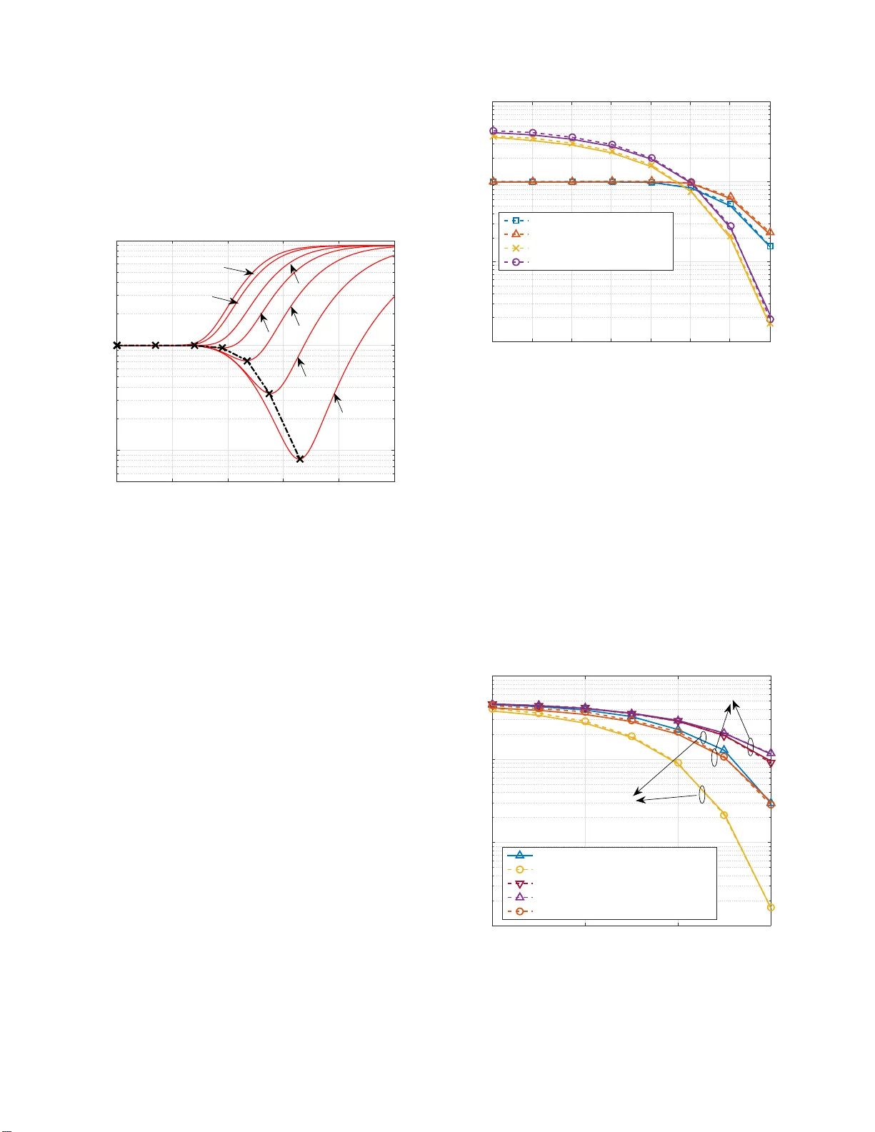
1 Interfer ing Channel Estimation in Radar -Cellular Coe xistence: Ho w Much Informa tion Do W e Need? Fan Liu, Student Me mber , IEEE, Adrian Ga rcia -Rod riguez, Membe r , IEEE, Christos Mas ouros, Sen ior Membe r , IEEE, and Giov anni Geraci, Member , IEEE Abstract —In this paper , we fo cus on the coexistence between a MIMO radar and cellular b ase stations. W e study the interfering channel estimation, where the radar is operated in th e “search and track” mode, and the BS r eceiv es the in terference from the radar . Unlike the con ventional methods where the radar and the cellular systems fully cooperate with each other , in this work we consider that they are uncoordinated and the BS needs to acquire the interfering chann el st ate information (ICSI) b y exploiting the radar probing wa ve for ms. For completeness, both the line-of- sight (LoS) an d Non-LoS (NLoS) ch annels ar e considered in the coexistence scenario. By further assuming that t he BS has limited a priori knowledge about the radar wave for ms, we propose sev eral hypothesis testing methods to identify the working mode of the radar , and then obtain th e ICSI through a variety of channel estimation schemes. Based on the statistical theory , we analyze the th eoretical performa nce of both the hypothesis testing and th e channel estimation methods. Finally , simulation results verify th e effectiveness of our theoretical analysis and demonstrate t hat the BS can effectively estimate the interfering channel even with limited information from the radar . Index T erms —Radar interfering channel estimation, Radar - communication coexistence, spectrum sharing, hypothesis testing, search and track. I . I N T RO D U C T I O N R ECENT years have witnessed an explosive gr owth of wireless services an d d evices. As a conseq uence, the frequen cy spectrum ha s beco me o ne of the m ost valuable resources. Since 20 15, mobile network op erators in the UK have been req u ired to pay a comb ined an nual total of £ 8 0.3 million for the 900MHz an d £ 119.3 million f or the 1800MHz bands [1]. G iven the crowdedness within the sub-1 0GHz band, policy regulato rs and network p roviders are now seeking for the oppor tunity to r e u se spectrum curren tly restricted to other applications. Inde e d, the f r equency ban ds occu pied for radar are among the b est candid ates to be shared amo ng various commun ication systems in the near future [2]–[5]. A. Existing Appr o aches Aiming for realizing th e spectral coexistence o f radar and commun ication, existing con tr ibutions mainly focus on m iti- gating the mutual interfere nce between the two systems by use This work has been submitted to the IEEE for possible publication. Copyri ght may be transferred without not ice, after which this ve rsion may no longer be accessibl e. F . Liu and C. Ma souros are with the Dep artment of Electro nic a nd Electric al Engineeri ng, Univ ersity College London, London, WC1E 7JE, UK. (e-mail : fan.li u@ucl.ac .uk, chris.masouros@ieee .org). A. Garcia- Rodriguez and G. Geraci are with Nokia Bell Labs, Dublin 15, Ireland. (e-mail: a.garciarodrigue z.2013@iee e.org, dr .giov anni.ge raci@gmai l.com). of pr ecoding/b eamform ing tech niques [ 6]–[10]. Su ch efforts can be fou nd in the pioneer in g work of [7], in wh ich the radar signals are precod ed b y a so-called null-space projector (NSP), and thu s the in terference ge n erated to the com m unication systems is zero-fo rced. T o achiev e a fav orable p erform ance trade-off, the NSP method is further im proved in [9], [10] via Singular V alue Decomposition (SVD) , wh e r e the interferen ce lev el can be adju sted considering the singular values o f the channel matrix. As a step furth er , more r ecent works have exploited co n vex optimization tec h niques for jo intly designing tr ansmit wa ve- forms/pre coders o f r adar and commun ication systems, such that certain perfo rmance metrics can be optimized [11]–[2 0]. For instance, in [13], the receive sign al-to-interf erence-p lus- noise ratio (SINR) of the r adar is maximized in the presence of both the clutters and the co mmunicatio n interfere n ce, while the c a pacity of the com munication system is gua ranteed. The in verse problem has been tackled in [14], where the commun i- cation rate h as been maximized subjec t to the r adar SINR con - straint, as well as the power budgets f or bo th systems. While the afor ementioned works are well-design ed via sophisticated technique s, it is in gen eral d ifficult for them to be app lied to current rada r application s, gi ven the fact that the governmental and military agencies a r e u nwilling to m ake majo r c h anges in their radar deploym ents, which may impo se hu ge costs on their financial b udgets [21]. He nce, a mor e p ractical approach is to develop transmission schemes at the com munication side only , where the rad ar is agnostic to the interfere nce or ev en the ope ration of th e commu nication system. In this line, [16] considers the coexistence between a MIMO ra dar and a BS perfo rming multi-user MI M O (MU-MIM O) downlink transmissions, in which the precoder of the BS is the o nly optimization variable. In [18], [19], the BS precod er has been further developed by explo iting the constructive multi-user interferen ce, which demo nstrates o rders-of -magnitud e p ower - sa vings. It is worth highlightin g th at precod in g based techniq ues require the knowledge of the interfering chann el either at the rada r or the communicatio n BS. In fact, per fect/imperfe c t channel state info rmation (CSI) assumptions are quite typical in the above works. T o ob tain such inform ation, the radar and the BS are suppo sed to f ully coo perate with each other an d transmit training sym bols, in line with conventional ch annel estimation methods. In [10], the MIMO radar need s to estimate the channe l based on the received pilot signals sent by the BS, which in evitably occu pies extra comp utational and signaling resources. Other works such a s [13] requ ire an all-in-on e 2 control center to be connecte d to both systems via a dedi- cated side inform ation link , which conducts the inform ation exchange and the waveform o ptimization. In pr actical scenar- ios, howe ver , the co ntrol center brings forward considerable complexity in th e system design, an d is thus difficult to implement. Moreover, since it is the cellular operator who exploits the spectrum of the radar, it is the p erform a nce of the latter that should be primarily gu aranteed, i.e . , the radar resources should be alloc ated to target d etection rather than obtaining the CSI. Unfortunately , many existing contributions failed to addre ss this issue, and, to the best of o u r kn owledge, the chan n el estimation approaches tailored for the radar- cellular coexistence scen arios remain widely u nexplored. In light of the a b ove drawbacks regarding the CSI acquisition, the natural q uestion is, 1 ) is it possible to estimate the chan nel when there is limited cooperation between the radar an d the communica tion systems? And if so, 2) h ow much information do we need for the estimation? B. The Contribution of Our W ork This pap er aims at answering the above issues, where we focus on inte r fering channel estimation betwee n a M IMO radar and a MI MO BS: 1) T o co pe with the first issue above, we her eby p ropose to exploit th e radar p robing waveforms for estimating the interferin g cha n nel. I n this case the r adar does not need to send training symbols o r estimate the channel by itself, and thus the need for co operatio n is f ully eliminated. Follo win g the classic MI MO r adar literature [22], [23], we assum e that the rada r h as two working modes, i.e., searching and tracking. In the search mode, the r adar transmits a spatially orthog onal waveform, which form ulates an omn i-direction al beampattern for searching potential targets over th e whole angula r d o- main. In the track mo de, the radar transmits dir e c tional wa veforms to track th e target located at the an g le of interest, and thus to obtain a more accurate o bservation. In the meantim e , the BS is tr ying to estimate the channel based on the period ically received radar interference , which is tied to th e ra d ar’ s duty cycle. As the searching and tra c king wav eforms are rando m ly transmitted, we propo se to identify the operation mo de of the r adar by use of the hypo th esis testing appro ach, and then estimate the channel at the BS. 2) T o answer th e second question raised above, we furthe r in vestigate different c a ses u nder both L o S an d NLoS channels, where different levels of prior i knowledge about the radar wa veforms are assumed to be kn own at the BS, i.e., from f u ll k n owledge of sear ching and tracking wa vefo rms b y the BS, to kn owledge of search- ing waveform only , to a fu lly agnostic BS to the radar wa veforms. From a r ealistic per spectiv e, the secon d and the th ird cases are more likely to appear in pr a c tice while the first case serves as a perf ormance b enchmark . According ly , the theoretical pe r forman ce analy sis of the propo sed approach es are provided. Ă Ă Radar TX Interfering Channel Comms RX (a) Ă Ă Radar TX Interfering Channel Comms RX (b) Fig. 1. MIMO Radar and BS coexist ence. (a) Radar search mode; (b) Radar track mode. For the sake of clarity , we summarize b elow th e con tr ibu- tions o f this p aper: 1) W e consider the interferin g channel estimatio n for the coexistence of rad ar and cellu la r, where the radar prob- ing wa veform s are exploited to obtain ICSI at the BS. 2) W e propose hy pothesis testing appro aches for the BS to identify the o p eration mode of the radar, based on the limited priori in f ormation available at the BS. 3) W e analyze the the o retical performan ce of the prop osed detectors and estimators, whose effectiveness is further verified via numer ical results. The remainder of this paper is arranged as follows. Section II introduces th e system m odel, Sectio n I II and Sectio n IV propo se in te r fering cha nnel estimation appro a ches fo r NLoS and LoS scenarios, respectively . Sub sequently , Section V an- alyzes the theoretical perfo rmance of th e pro p osed sch emes, Section VI p rovides the corresp o nding numer ical results, and finally Section VII conclude s the paper . Notations : Un less o therwise spec ified , matrices are denoted by bo ld u ppercase letters (i.e. , X ), vectors are r e p resented by bold lowercase letters (i.e., z ), an d scalar s are denoted b y normal fo nt (i.e., ρ ) . tr ( · ) and vec ( · ) den ote the trace and the vectorization oper ations. ⊗ d enotes the Krone cker pr o duct. k·k and k·k F denote the l 2 norm and the Frobenius nor m. ( · ) T , ( · ) H , and ( · ) ∗ stand fo r tra nspose, Hermitian transpose an d complex co n jugate, respectively . I I . S Y S T E M M O D E L As shown in Fig. 1, we consider a MIMO radar with M t transmit antennas and M r receive antennas that is detecting targets located in the far field. For simplicity , we assume that 3 Fig. 2. Radar wo rking mode - “search and track” and operations perfo rmed by the communicat ions BS. the MIMO rad ar employs the same anten na array for b oth transmission and reception , and den ote M t = M r = M . Meanwhile, an N -antenna BS o p erating in the same freq uency band is receiving in terference from th e radar an d tryin g to acquire the ICSI between them. Below we pr ovide the system models for b oth the radar and the BS. A. Rad ar Sig nal T ransmission - S ear ch and T r ack It is widely k n own that by emp loying inco herent wav eforms, the MIMO radar achieves highe r Degrees of Freed om (DoFs) and better perfo r mance tha n the co n ventional phased-ar ray radar that transmits correlated wav eforms [22]. By denotin g the MIMO rad ar pr obing wa veform a s X ∈ C M × L , its spatial covariance matrix can be giv en as [22]–[2 6] R X = 1 L XX H , (1) where L is th e leng th of the rad ar pulse. Throu ghout the paper we consider L ≥ N ≥ M > 2 , an d assume uniform line a r arrays (ULA) at bo th th e r adar and the BS. Th e corr esponding beampatter n c a n be thu s g iv en in the form [22]– [ 26] P d ( θ ) = a H ( θ ) R X a ( θ ) , (2) where θ deno tes the azimuth angle, an d a ( θ ) =  1 , e j 2 π ∆ sin( θ ) , ..., e j 2 π ( M − 1)∆ sin( θ )  T ∈ C M × 1 is the steer- ing vector of the transmit antenn a array with ∆ being the spacing b etween adjacen t antennas nor m alized by the wa ve- length. When th e orthog onal wa veform is tran sm itted by th e MIMO radar, it fo llows that [24], [2 7] R X = P R M I M , (3) where P R is the total tr ansmit power of the radar, and I M is the M - dimensiona l identity matrix. It is easy to see fr om (2) that the covariance matr ix (3) generates an omn i-direction a l beampatter n , which is ty pically used for sear chin g whe n there is limited inf ormation ab out the target locations [22]. Once a target is d etected, the radar switches to the trac king mode , where it will no longer transmit orthogon al waveforms and will generate a direc tio nal beamp attern that p oints to the specific location, thus obtaining a more a c curate observation. This, however , results in a non - orthog onal transmission, i.e., R X 6 = P R M I M . In this paper, we assume that the radar ado p ts both the search ing a nd tracking mod es subject to a probability transition mod el. This mod el is illustrated in Fig. 2 a nd can be su mmarized as follows [2 8]: Assumption 1 : At the i -th pulse r epetition in terval (PRI) of the rad ar , the prob ability that the radar is opera tin g at the tracking mo de is P ( i − 1) D , wh ere P ( i − 1) D is the ta rget detection probab ility of th e ( i − 1) -th PRI. The above assumption entails th at the MIMO radar ch anges its pro bing wa veform X randomly within eac h PRI, wh ic h makes it challen ging for the BS to estimate the inter fering channel between the m . B. Interfering Channel Model The interfer ing chan nel be tween the BS an d the radar could be characterized throug h different models, dependin g on their specific p o sitions. For instance, the military and weath er radars are typically located at high-altitude places such as top of th e hills, in which case the channel between the BS an d radar is likely to be a Lin e-of-Sigh t (L oS) channe l. On the other hand, if the radar is used f o r mo nitoring th e low-altitude flying objects (such as d rones) o r the urb an traffic, it is usually deployed in urban areas at similar heights than the BS, thus resulting in a Non-Line- of-Sight (NLoS) cha n nel. For completen ess, we will discuss both cases in this p a p er . Since bo th the radar and th e BS are located in fixed p ositions, we also adop t the following assumption : Assumption 2 : For the LoS coexistence scen ario, we assume that th e inter fering chan nel fro m the radar to the BS is fixed. For the NLoS coexistence scenario, we assume the interferin g channel is flat Rayleigh fading, and remains unchan ged du r ing se veral ra dar PRIs. C. BS Signal Reception Mode l Denoting the interfering channel as G ∈ C N × M , the received signal matr ix at the BS can be given as Y = GX + W , (4) where W = [ w 1 , w 2 , ..., w L ] ∈ C N × L is the noise matrix, with w l ∼ C N ( 0 , N 0 I N ) , ∀ l . In th e pr oposed hypothe sis testing framework, the n oise power N 0 plays an imp ortant role for no r malizing the test statistic. Note that wh en radar keeps silent, the BS will recei ve no thing b ut the noise, and N 0 can be measured at this stage. Sin c e the radar antenna num b er and its transmit power are fixed parame ters, they can also be easily known to th e BS oper ators. T herefor e , it is reasona ble to adopt the f ollowing assumption: Assumption 3 : T h e BS knows the value of N 0 , M an d P R . In or der to estimate the chan n el and the noise power N 0 , the BS need s to k now when is ra d ar transmitting, i.e., it must synchro n ize its clock with the r a dar pu lses. As sho wn in Fig. 2, d uring o ne PRI, the radar only transmits f or a p ortion of the time, typ ically below 10%, and employs the remaining 90 % for r eceiving, d uring which the radar rem ains silent. Such a ratio is called du ty cyc le [1 4]. By exploiting th is pro perty , the BS is able to b lindly estimate the b eginning and the e n d of a radar pu lse by some simple meth ods, such as en ergy detection. Note th a t fo r th e NL oS ch annel scen ario, there will be r a ndom time-spr e ad delays within each pulse, which makes 4 the synch ronization inaccurate. Howe ver , since we assume a flat fading chan nel in the NLo S case, the time-spread delay will be contain ed within one snapsh ot of th e radar, which results in negligible error s [ 29]. W e summ arize the ab ove throug h the following assumption: Assumption 4 : Th e BS can perfe ctly synch ronize its clock with the radar pulses, i.e., it is ab le to know the beginnin g an d the end of each radar p ulse. D. Chann el Estimation Pr o cedur e In light of the above discussion, we summarize below the channel estimation pr o cedure at the BS: 1) Sy nchron ize the system clock with the radar transmitted pulses. 2) I dentify the working mode of th e radar based on th e received radar interfer e nce, i.e., whether the rad a r is searching or track ing. 3) E stimate the interferin g chann el by explo iting the limited knowledge about the ra d ar w av eforms. In the f ollowing, we will develop se veral appr oaches for the BS to acquire the ICSI when rad a r is ra ndomly chan ging its probin g wa veform. W e will first consider the NLoS chann e l case, and th en th e Lo S channel case. I I I . N L O S C H A N N E L S C E N A R I O Consider the ideal case wh ere the BS k n ows exactly th e wa veform sent by the rada r in each PRI. Recalling (4), the well-known max imum likeliho od estimatio n (MLE) of th e channel G is given as [ 30] ˆ G = YX H  XX H  − 1 , (5) which is also known as the Least-Square s estimation (LSE) for G . Un fortunately , the BS is no t ab le to identify which wa veform is tran smitted, since th e radar changes its wa veform random ly at each PRI. Hen ce, (5) can no t be directly ap plied and it is difficult to estimate th e c hannel dire ctly . In this section, we discuss several cases where different levels of knowledge about th e radar wa vefo rms are a vailable at the BS. At each level, we pro pose specifically tailored ap proach e s to acquire the ICSI. A. BS Knows the Searc hing and T racking W aveforms - Gen- eralized Likelihood Ratio T est (GLRT) In th is referen ce case, we assume that the BS knows both the searching and the tr acking wa veforms that the radar may transmit at th e i -th PRI, which we denote as X 0 and X 1 , respectively . Sin ce X 0 is orthogo nal, we h av e 1 L X 0 X H 0 = P R M I M ⇒ X 0 X H 0 = LP R M I M . (6) Before estimatin g the ch a nnel, the BS needs to identify which wa veform is transmitted based on the received no isy data Y ∈ C N × L . This leads to th e fo llowing hypoth esis testing (HT) problem [31] Y = ( H 0 : GX 0 + W , H 1 : GX 1 + W . (7) As per Assumptio n 1 , th e prio ri pro babilities o f the above two hypoth eses can be given as P ( H 0 ) = 1 − P ( i − 1) D , P ( H 1 ) = P ( i − 1) D . (8) The HT prob lem (7) can be solved via the gen eralized likeli- hood ratio test (GLR T), which is given by [31] L G ( Y ) = p  Y ; ˆ G 1 , H 1  P ( H 1 ) p  Y ; ˆ G 0 , H 0  P ( H 0 ) = p  Y ; ˆ G 1 , H 1  P ( i − 1) D p  Y ; ˆ G 0 , H 0   1 − P ( i − 1) D  H 1 ≷ H 0 γ , (9) where γ is the detection threshold , p  Y ; ˆ G , H 1  and p  Y ; ˆ G , H 0  are the likelihoo d fun ctions (LFs), for the two hypoth eses respecti vely , and can be given in the form p  Y ; ˆ G , H 0  = ( π N 0 ) − N L exp  − 1 N 0 tr   Y − ˆ GX 0  H  Y − ˆ GX 0   , (10) p  Y ; ˆ G , H 1  = ( π N 0 ) − N L exp  − 1 N 0 tr   Y − ˆ GX 1  H  Y − ˆ GX 1   . (11) In the ab ove expressions, ˆ G 1 and ˆ G 0 are the ML E s under H 1 and H 0 , which ar e ob tained as ˆ G 1 = YX H 1  X 1 X H 1  − 1 , (12) ˆ G 0 = YX H 0  X 0 X H 0  − 1 = M LP R YX H 0 . (13) Overall, once the BS de ter mines which hyp othesis to choose based on Y , it can successfully estimate th e channel b y use o f (12) or (13). Howe ver , it can be obser ved that the GLR T detector in ( 9) r equires the d e tection pro bability P ( i − 1) D to be known to the BS, which is impossible in practice. Therefo re, the detec tor (9) can on ly serve as th e optimal performance bo und . Since the actual P ( i − 1) D is unknown to the BS, the re a sonable ch oice for the pr io ri pro babilities is P ( H 0 ) = P ( H 1 ) = 0 . 5 , namely P ( i − 1) D = 0 . 5 . W e can then apply the similar G L R T pr o cedure for solv in g th e HT pro b lem. The test statistic in (9) is thus simplified as L G ( Y ) = p  Y ; ˆ G 1 , H 1  p  Y ; ˆ G 0 , H 0  H 1 ≷ H 0 γ . (14) B. BS Knows On ly the Sea r ching W aveform - Ra o T est In a realistic scenario, the tracking wa veform X 1 may vary from p ulse to pu lse. This is because the target to be detected may move very fast, which results in rap id ch anges in its parameters such as the distance, velocity and the azimuth angle. Hen ce, it is far from r ealistic to assume the BS knows 5 X 1 , not to men tion P D (in fact, both q uantities ar e on ly determined after a target is detected). Nev ertheless, as an omni-d ir ectional searchin g wav eform, there is no reason for X 0 to be chan ged r apidly . Indeed , in so me cases, the radar may only u se one waveform for omn i-searching . Based on the above, to assume tha t the BS only knows X 0 seems to be a more pr actical choice 1 . In th is case, th e HT pr oblem (7) can be r ecast as H 0 : X = X 0 , G , H 1 : X 6 = X 0 , G . (15) In (15), th e chann el to be estimated is called the nuisanc e parameter [31]. Remark 1: At first glanc e , the GLR T pro cedure seems to be applicable to (15) as well. Howe ver, no te that to o b tain the MLE of G un der H 1 is equiv a len t to solving the following optimization problem min G , X k Y − GX k 2 F s.t. k X k 2 F = L P R , (16) where the constra in t is to ensure th e power budget o f th e radar-transmitted wav eform. While the above p roblem is non- conv ex, it yields trivial solutions that achieve zero with a high p robability . This is becau se the problem (1 6) is likely to have more th an enoug h DoFs to ensure that Y = GX , since G is unco n strained, and X can be a lw ays scaled to satisfy the nor m constraint, where the scaling factor can be incorpo rated in G . Theref ore, the likeliho o d function under H 1 will always be greater than that of H 0 , which makes the HT design m eaningless. Realizing the fact above, we propose to use th e Rao test (R T) to solve the HT problem (15), which does not need the MLE under H 1 . Based o n [ 3 2]–[34], let us define Θ =  vec T ( X ) , vec T ( G )  T ,  θ T r , θ T s  T . (17) Then, the R T statistic for the complex-valued parameters can be g iv en in the form T R ( Y ) = 2 ∂ ln p ( Y ; Θ ) ∂ vec ( X )     T Θ = ˜ Θ h J − 1  ˜ Θ i θ r θ r ∂ ln p ( Y ; Θ ) ∂ vec * ( X )     Θ = ˜ Θ H 1 ≷ H 0 γ , (18) where ˜ Θ = h θ T r , ˆ θ T s i T = h vec T ( X 0 ) , v ec T  ˆ G 0 i T is the MLE u nder H 0 , an d h J − 1  ˜ Θ i θ r θ r is the uppe r-left par tition of J − 1  ˜ Θ  , with J ( Θ ) being the Fisher I nformatio n Matrix (FIM). Unlike the GLR T , the Rao test only lets the BS deter mine if the radar is u sing the searc h ing mode, i.e., whether th e orthog onal waveform matrix X 0 is transmitted in the cu rrent radar PRI. In that case, the BS could obtain the MLE of the channel by use of (13). Otherwise, th e BS is required to wait until an o rthogo n al wa vefo rm is transmitted by th e radar . 1 At this stage we note the fact that such information exchange can be easily performed once prior to transmission, since the searching wa ve form of the radar remains unchange d. In contrast, con vent ional training based techniques require the radar or the BS to frequently send pilot symbols, which entai ls a much tighte r cooper ation between both systems. C. Agnostic BS W e n ow conside r the hardest case th at the BS does not know any of the wa veforms transmitted by th e radar . In this case, the BS still knows that XX H = LP R M I M for an omn i-directional radar transmission . Th erefore , the HT problem in (15) can be recast as H 0 : XX H = LP R M I M , G , H 1 : XX H 6 = LP R M I M , G . (19) Remark 2: At first glan ce, we m ight be able to app ly a generalized R T to solve the HT proble m , w h ere bo th th e tru e values of G and X 0 are replac e d b y their M LEs. This is because X 0 is also unkn own to the BS. Note that to obtain the MLEs of these two parameters is equiv alent to solving the following optimizatio n problem min G , X k Y − GX k 2 F s.t. XX H = LP R M I M . (20) Again, the above prob lem will unf ortunately yield trivial so- lutions and make the HT design mean ingless. This is b ecause X can be viewed as a grou p of orth ogona l ba sis, a n d the uncon stra in ed G spa ns the who le space, which makes any giv en Y achievable with a high probab ility . The above remark inv olves that it is challengin g to blindly estimate th e I CSI for an agnostic BS under the NLoS channel scenario. Instead, we will show in the next section that blind channel estimation is feasible for the LoS chann el scenario. I V . L O S C H A N N E L S C E N A R I O In this section, we consider the scen a rio that the interferin g channel between radar and BS is a Lo S chann el, wh ere the received signal matr ix at the BS is given by Y = α b ( θ ) a H ( θ ) X + W , (21) where α r epresents the large-scale fading factor , θ is th e angle of arrival (Ao A) from the radar to the BS, b ( θ ) =  1 , e j 2 π Ω sin( θ ) , ..., e j 2 π ( N − 1)Ω sin( θ )  T ∈ C N × 1 is the steering vector o f the BS antenna arra y , with Ω being the normalized spacing, and a ( θ ) is ra dar’ s steerin g vector defin e d in Sec. II-A. Sinc e the ULA geom etry of the radar is fixed, we assume that the BS k nows the spacing b etween th e a d jacent antennas of rad ar . Hence, the chan n el p arameters that need to be e stimated at th e BS are α and θ . Adopting the ideal assumptio n that the BS h as instantan e o us knowledge of the rada r-transmitted waveform X in each PRI, the MLEs of the two parameters co u ld be obtained by so lv ing the o ptimization problem min α,θ   Y − α b ( θ ) a H ( θ ) X   2 F . (22) Note th at if θ is fixed, the MLE of α can be gi ven as ˆ α = b H ( θ ) YX H a ( θ ) L k b ( θ ) k 2 a H ( θ ) R X a ( θ ) = b H ( θ ) Y X H a ( θ ) N L a H ( θ ) R X a ( θ ) , (23) 6 which suggests th at the ML E of α d epends o n th a t o f θ . Substituting (23) into the objective function of (22), the MLE of θ can be th u s gi ven by ˆ θ = ar g min θ f ( Y ; θ , X ) , (24 ) where f ( Y ; θ , X ) =     Y − b H ( θ ) Y X H a ( θ ) b ( θ ) a H ( θ ) X N L a H ( θ ) R X a ( θ )     2 F . (25) While (25 ) is no n-conve x, the op timum can be easily obtain ed throug h a 1-dimensional search over θ . A. BS Knows the Sea r chin g and T racking W aveforms - GLRT By assuming that th e BS knows both X 0 and X 1 , the HT problem (7) ca n b e ref ormulated as Y = ( H 0 : α b ( θ ) a H ( θ ) X 0 + W , H 1 : α b ( θ ) a H ( θ ) X 1 + W . (26) The GLR T detector can be aga in ap plied to th e Lo S channel, in which case the likelihood fu nctions under the two hyp otheses are g iv en a s p  Y ; ˆ θ 0 , H 0  = ( π N 0 ) − N L exp  − 1 N 0 f  Y ; ˆ θ 0 , X 0   , p  Y ; ˆ θ 1 , H 1  = ( π N 0 ) − N L exp  − 1 N 0 f  Y ; ˆ θ 1 , X 1   , (27) where f is defined in (25), and ˆ θ 0 and ˆ θ 1 are th e MLEs of θ under the two hypoth eses, respectively . By r ecalling (9), the GLR T detector can be expressed as L LoS G ( Y ) = 1 N 0  f  Y ; ˆ θ 0 , X 0  − f  Y ; ˆ θ 1 , X 1  H 1 ≷ H 0 γ . (28) The analytic distribution for (2 8) is n ot obtainab le , since there is n o closed-form so lu tion of ˆ θ und er both hypo theses. B. BS Kno ws Only the Sea r ching W a veform - Energy Detec- tion Similar to the NLoS chann el case, a more practical as- sumption is to consider that the BS k nows on ly the searching wa veform X 0 . I n th is case, the GLR T detector is no longer applicable and the HT is gi ven by H 0 : X = X 0 , α, θ, H 1 : X 6 = X 0 , α, θ. (29) At first g lance, it seems that th e Rao dete c to r (18) can be trivially extended f rom th e NLo S channel scen ario to the LoS case. Nev ertheless, the fo llowing pr oposition puts an en d to such a po ssibility . Proposition 1. The Rao test doe s not exist for the scenario of the LoS channel. Pr oo f. See Appendix A.  The algebraic explan ation be h ind Proposition 1 is intuitive. As shown in (2 1), by mu ltiplying the rank -1 LoS chan nel Fig. 3. Searching and tracking beampatt erns of the MIMO radar . to the radar wa veform, the latter is map ped to a rank-1 subspace, which leads to seriou s in formation losses and yield s a non-inv ertible FIM. Recalling (18), the Rao test requires to compute the in verse of the FIM . Hence, it simply does not work in this specific c ase. T o resolve the aforeme ntioned issue, we consider an energy detection (ED) appr oach f or the LoS chann el. According to (21), th e average power of the received r a dar sign al is given as P LoS = E  tr  YY H  = E   tr  | α | 2 b ( θ ) a H ( θ ) XX H a ( θ ) b H ( θ ) + W W H  + 2 Re  tr  α b ( θ ) a H ( θ ) XW H    = E  tr  | α | 2 b ( θ ) a H ( θ ) XX H a ( θ ) b H ( θ ) + WW H  ≈ 1 L tr  | α | 2 b ( θ ) a H ( θ ) XX H a ( θ ) b H ( θ )  + N N 0 = | α | 2 P d ( θ ) tr  b ( θ ) b H ( θ )  + N N 0 = N | α | 2 P d ( θ ) + N N 0 , (30) where P d ( θ ) is the radar tra n smit beampattern defined in (2), and the approx imation in the four th line of ( 30) is b a sed on the L aw of Large Nu m bers. From (30), it is obvious that the received power at the BS is prop ortional to the rad ar’ s transmit po wer at the angle θ . If the searching waveform X 0 is tr ansmitted, we h av e P d ( θ ) = P R M a H ( θ ) I M a ( θ ) = P R , (31) which sugg ests that the BS will receive equal power at each angle θ . On the other h and, if th e tra cking wav eform X 1 is transmitted, mo st of the power will focu s at th e mainlob e, while less power will be distributed among the sidelob es, in which case th e BS r eceiv es high power when it is lo cated at the mainlobe of the radar, an d m uch lower power at other a n gles. According to the aforementio ned observations, in this pa per we let the BS d e fine two power measurement thresh olds to 7 determine whether the radar is in searc h ing o r tracking mode. As shown in Fig . 3 2 , the BS ch o oses H 0 if the received power falls between the two pro posed thresholds, and it chooses H 1 otherwise. Accordingly , th e ED detector can be given as T E ( Y ) = 1 L tr  YY H  ∈ [ γ , η ] → H 0 , T E ( Y ) = 1 L tr  YY H  ∈ (0 , γ ] ∪ [ η , + ∞ ) → H 1 , (32) where γ and η ar e the two p ower thresho ld s. Remark 3: Note that the perf ormance of the detecto r in (3 2) depend s on th e size of the am biguity regions sh own in Fig. 3. By nar r owing the distance betwee n γ and η , th e d etector trades-off the tolerance of the noise with the ambig uity area. By using the ED detector, the BS could choo se from the two h y potheses witho ut kn owing b oth waveforms. Once H 0 is chosen, the BS ca n estimate the AoA b y finding the m inimum of f ( Y ; θ , X 0 ) . C. Agn ostic BS Finally , we consider th e h ardest ca se wh ere th e BS does not know either th e searching o r track in g wav eform. Note that the energy detecto r (32) still works in this case, as it does not requ ire any inform ation about X 0 or X 1 . The remain ing question is how to estimate the channel. In o rder to do so, we first note that fo r the case of o mni-direc tio nal transmission we have P d ( θ ) = P R M a H ( θ ) I M a ( θ ) = P R , (33) in which ca se (31) can be re written as P LoS = E  tr  YY H  ≈ 1 L tr  YY H  ≈ N P R | α | 2 + N N 0 . (34) From (34), it follows that | α | 2 ≈ tr  YY H  LN P R − N 0 P R , (35) which can be used for estimating the ab solute value of α . I t can be fu rther observed that f or the omni-dire c tional transmission , we also h av e 1 L YY H = | α | 2 P R M b ( θ ) a H ( θ ) I M a ( θ ) b H ( θ ) + ˜ W = | α | 2 P R b ( θ ) b H ( θ ) + ˜ W , (36) where ˜ W is the noise matrix. T h e LSE of θ can be th us given by ˆ θ = ar g min θ     YY H LP R − | α | 2 b ( θ ) b H ( θ )     2 F . (37) Overall, once H 0 is cho sen by the en ergy d etector (32), one can estimate | α | 2 and θ by (3 5) and (37) respectively , ev en without any knowledge about th e rada r wa veforms. W e remark that, sin c e the n oise m a trix ˜ W is no longer Gaussian distributed, (35) and (37) are not MLEs o f th e par a meters. For clarity , we summa r ize the pr oposed app roaches for different scenarios in T able. I. 2 The tracking beampa ttern in Fig. 3 is generated based on the con vex optimiza tion method in [22], which we show in (73) in Sec. VI. T ABLE I P R O P O S E D A P P RO AC H E S F O R D I FF E R E N T S C E N A R I O S NLoS Channel LoS Channel BS Knows Both W aveforms GLR T GLR T BS Knows Searching W avef orm Rao T est Energ y Detecti on Agnostic BS None Energy Detection V . T H E O R E T I C A L P E R F O R M A N C E A NA L Y S I S In this section, we provide the theoretical p erforma n ce analysis for the pro posed hypoth esis testin g and c hannel esti- mation app roaches. With this p urpose, we use decision error probab ility and the mean squared error (MSE) as performan ce metrics. A. GLRT for NLoS Chann els T o analyze the perf ormance of the GLR T detecto r , the M LEs of the unknown parameter s un der d ifferent hypo theses m ust be derived in clo sed-form s. Wh ile we consider GLR T for both NLoS an d L o S chan nels in the previous discussion, the closed- form MLE of the AoA is no t obtainable for the Lo S channel. Therefo re, we w ill only analyze the GLR T p erforman ce for the NLoS channel in this subsection. Firstly , let us substitute (12) and (13) into (10) an d ( 11), wh ich yield p  Y ; ˆ G 0 , H 0  = ( π N 0 ) − N L exp  − 1 N 0 tr   Y − ˆ G 0 X 0  H  Y − ˆ G 0 X 0   = ( π N 0 ) − N L exp  − 1 N 0 tr  Y  I − M LP R X H 0 X 0  Y H  , (38) and p  Y ; ˆ G 1 , H 1  = ( π N 0 ) − N L exp  − 1 N 0 tr   Y − ˆ G 1 X 1  H  Y − ˆ G 1 X 1   = ( π N 0 ) − N L exp  − 1 N 0 tr  Y  I − X H 1  X 1 X H 1  − 1 X 1  Y H  . (39) T a k ing the logar ithm of (9) we obtain ln p  Y ; ˆ G 1 , H 1  P ( i − 1) D p  Y ; ˆ G 0 , H 0   1 − P ( i − 1) D  = 1 N 0 tr  Y  X H 1  X 1 X H 1  − 1 X 1 − M LP R X H 0 X 0  Y H  − ln 1 − P ( i − 1) D P ( i − 1) D ! H 1 ≷ H 0 γ 0 . (40) Finally , the GLR T detector can be given as L G ( Y ) = 1 N 0 tr  Y  X H 1  X 1 X H 1  − 1 X 1 − M LP R X H 0 X 0  Y H  H 1 ≷ H 0 γ = γ 0 + ln 1 − P ( i − 1) D P ( i − 1) D ! . (41) 8 T R ( Y ) = 2 N 0 tr  I L − M LP R X H 0 X 0  Y H YX H 0  X 0 Y H YX H 0  − 1 X 0 Y H Y  H 1 ≷ H 0 γ . (51) Note that both X H 1  X 1 X H 1  − 1 X 1 and M LP R X H 0 X 0 are pro je c - tion matrices [30]. Th e physical meaning of (41) is intu iti ve, i.e., to project th e recei ved sign al onto th e ro w spaces o f X 1 and X 0 respectively , and to compute the difference between the lengths of the p rojections to decide w h ich hy pothesis to choose. Letting P ( i − 1) D = 0 . 5 , we hav e ln  1 − P ( i − 1) D P ( i − 1) D  = 0 and γ = γ 0 , which r e presents the case that P D is u nknown. W e now der i ve the Cum ulativ e Distribution Function (CDF) of L G . Defin ing A = X H 1  X 1 X H 1  − 1 X 1 , B = M LP R X H 0 X 0 , ˜ y = vec  Y H  √ N 0 , D = I N ⊗ ( A − B ) , (42) it follows that L G ( Y ) = ˜ y H ( I N ⊗ ( A − B )) ˜ y = ˜ y H D˜ y . (43) If D is an idempotent matr ix, then th e test statistic subjects to the non-c e n tral chi-squ ared distribution [ 30]. While both A and B are idem p otent, it is not clear if their difference is still idempoten t. Moreover, their is no guarantee that D is semidef- inite. Hen ce, D is an indefinite matrix in general, which makes L G an indefinite quadratic fo rm (IQF) in Gaussian variables. Giv en the non - zero mean value of ˜ y , L G becomes a non- central Gau ssian I QF , which is k nown to have no closed-form expression for its CDF [35], [3 6]. Based on [ 3 7], here we consider a so-called saddle-po int meth od to approx imate the CDF of the test statistic. It is clear th a t ˜ y ∼ C N ( b , I N L ) , where b =    H 0 : vec  X H 0 G H  . p N 0 , H 1 : vec  X H 1 G H  . p N 0 , (44) which are th e mean values for ˜ y under H 0 and H 1 respec- ti vely . Let us d enote the eigen value decom p osition of D as D = QΛQ H , where Λ = diag ( λ 1 , λ 2 , ..., λ N L ) contains the eigenv alu es. Based on th e sadd le - point appro ximation [37], the CDF of L G is giv en as P ( L G ≤ γ ) ≈ 1 2 π exp ( s ( ω 0 )) s 2 π | s ′′ ( ω 0 ) | , (45) where s ( ω ) = ln  e γ ( j ω + β ) e − c ( ω ) ( j ω + β ) det ( I + ( j ω + β ) Λ )  , (46) c ( ω ) = N L X i =1   ¯ b i   2 − N L X i =1   ¯ b i   2 1 − ( j ω + β ) λ i , (47) ¯ b = Q H b =  ¯ b 1 , ¯ b 2 , ..., ¯ b N L  T . (48) The above results hold for any β > 0 . ω 0 is the so-called saddle point, which is the solu tio n o f th e following equation s ′ ( j ω ) = − 1 ( − ω + β ) − N L X i =1 λ i 1 + λ i ( − ω + β ) + γ − N L X i =1   ¯ b i   2 λ i (1 + λ i ( − ω + β )) 2 = 0 , (49) where ω = j ( β + p ) . It ha s been proved that (49) ha s a single real so lution on p ∈ ( −∞ , 0) [37], which can be nu merically found through a 1-dim ensional searching . At the i -th PRI, it is natural to measure the perform a nce of GLR T by use of the decision er ror prob ability g iven th e CDF of L G , which is ob tained as P ( i ) G = P ( L G ≥ γ ; H 0 ) P ( H 0 ) + P ( L G ≤ γ ; H 1 ) P ( H 1 ) = (1 − P ( L G ≤ γ ; H 0 ))  1 − P ( i − 1) D  + P ( L G ≤ γ ; H 1 ) P ( i − 1) D , (50) where the CDF of L G under each h ypothesis can be compu ted using the above equ a tions ( 45)-(49), by accord ingly su b stitut- ing the values o f b und er the two hy potheses, which are given in ( 44). B. Rao T est for NLoS Chan nels W e start from the following p r oposition. Proposition 2. Th e Rao detector for solving (15) is given by (51), shown at the top of this page. Pr oo f. See Appendix B.  It is clear from (51) that we do not need any info rmation about X 1 for solving the HT prob lem (15), which makes it a suitable detecto r for the practical scena rio where the BS only knows X 0 . While Y is Gaussian distributed, it is very difficult to an alytically de r iv e the CDF of (51) d ue to the highly no n- linear op erations in volved. By realizin g this, he r e we o nly focus o ur attention on a special c a se, wh e re th e d istribution becomes tractable. No te that if L ≥ M = N holds true, YX H 0 ∈ C N × N and X 0 Y H ∈ C N × N become the in vertible square matr ices w ith a high pr obability , in which ca se we h av e YX H 0  X 0 Y H YX H 0  − 1 X 0 Y H =   X 0 Y H  − 1 X 0 Y H YX H 0  YX H 0  − 1  − 1 = I N . (52) 9 It follows that T Rs ( Y ) = 2 N 0 tr  I L − M LP R X H 0 X 0  Y H Y  = 2 N 0 tr  Y  I L − M LP R X H 0 X 0  Y H  , 2 N 0 tr  YPY H  H 1 ≷ H 0 γ (53) is the Rao d etector u nder this special case. It c a n be seen that (5 3) is also a qu adratic fo rm in Gaussian variables. Interestingly , the matrix P = I L − M LP R X H 0 X 0 is a projection matrix, which projects any vector to the n u ll-space of X H 0 . Therefo re, we ha ve tr  GX 0 PX H 0 G H  = 0 , (54) which leads to tr  GX 1 PX H 1 G H  ≥ 0 = tr  GX 0 PX H 0 G H  . (55) The ab ove equ ations (54) and (55) can be viewed as the hypoth esis testing for the noise-fr e e scenario, where we see that the Rao detecto r ( 53) is effecti ve in differentiating th e two hy p otheses. By addin g the Gaussian noise to GX 1 and GX 0 , it c an be infer red that T Rs ( Y ; H 1 ) ≥ T Rs ( Y ; H 0 ) with a h igh pr obability in the high SNR regime, wh ich makes the detector (5 3) valid. Proposition 3. T Rs subjects to central a nd non -central chi- squar ed distrib utions und er H 0 and H 1 , r espe ctively , which ar e given as T Rs ∼ ( H 0 : X 2 K , H 1 : X 2 K ( µ ) , (56) wher e µ = 2 N 0 tr  GX 1  I L − M LP R X H 0 X 0  X H 1 G H  is the non-ce ntrality parameter , and K = 2 N ( L − M ) repr esents the DoFs of the distrib utions. Pr oo f. See Appendix C.  Similar to ( 5 0), the d ecision er ror pro bability at the i -th PRI for the special Rao detector ( 53) is given by P ( i ) Rs =  1 − F X 2 K ( γ )   1 − P ( i − 1) D  + F X 2 K ( µ ) ( γ ) P ( i − 1) D , (57) where F X 2 K and F X 2 K ( µ ) are the CDFs of central and non- central chi-squared distributions, respectiv ely . C. Chan nel Estimation P e rformance for NLoS Channels As discussed in Sec. I V , there are no closed-form solutions for the estimations of the Ao A under the LoS chan nel. Hence, we only consider the channel estimation performanc e for the NLoS channel case, where the MSE is u sed as the perfor mance metric. By den oting th e estimated channe l as ˆ G = YX H  XX H  − 1 , the squared error can be g iv en in the form φ =    ˆ G − G    2 F =    YX H  XX H  − 1 − G    2 F =     XX H  − 1 XY H − G H    2 F . (58) Let us define ¯ y = vec  Y H  ∼ C N  vec  X H G H  , N 0 I N L  , T = I N ⊗  XX H  − 1 X , ¯ g = vec  G H  . (59) Then, (58) can be simplified as φ = k T ¯ y − ¯ g k 2 . (60) Based on ba sic statistics and linear algeb ra, we also ha ve y eq , T¯ y − ¯ g ∼ C N  0 , N 0 TT H  , (61) where TT H = I N ⊗  XX H  − 1 X · I N ⊗ X H  XX H  − 1 = I N ⊗  XX H  − 1 . (62) Based o n the above, the MSE o f the cha nnel estimatio n can be o btained as E ( φ ) = E  k y eq k 2  = E  tr  y eq y H eq  = tr  E  y eq y H eq  = N 0 tr  I N ⊗  XX H  − 1  = N 0 N L tr  R − 1 X  . (63) In the case that the directional wa veform is transmitted , we have R X = 1 L X 1 X H 1 . For the orthogon al transmission , th e MSE can be given as E ( φ ) = N 0 N L tr  P R M I M  − 1 ! = N 0 M 2 N LP R . (64) It is clear fr o m (63) that th e MSE is determ in ed by the covariance matrix an d the length of the rad a r wav eforms, as well as the antenn a num b er at the BS. D. Energy Detection for Lo S Cha nnels In this subsection, we an alyze the perfo rmance of the energy detector ( 32). Fir st o f all, let u s re write (3 2) as 2 N 0 tr  YY H  = 2 ˜ y H ˜ y , (65) where ˜ y ∼ C N ( d , I N L ) is g i ven in (42), with d being d efined as d =    H 0 : vec  α ∗ X H 0 a ( θ ) b H ( θ )  . p N 0 , H 1 : vec  α ∗ X H 1 a ( θ ) b H ( θ )  . p N 0 . (66) Eq. (65) is the sum of the squared Gaussian v ariables, which subjects to the non-ce n tral chi-squ ared distribution [ 30]. Recall the pro o f of Pr o position 3. By replacing the matrix P in (89) as the identity matrix I L , we obtain th e no n-centrality parameter s under two hyp otheses as ε 0 = 2 | α | 2 N 0 tr  b ( θ ) a H ( θ ) X 0 X H 0 a ( θ ) b H ( θ )  = 2 | α | 2 N LP R N 0 , (67) ε 1 = 2 | α | 2 N 0 tr  b ( θ ) a H ( θ ) X 1 X H 1 a ( θ ) b H ( θ )  . (68) 10 The DoFs of both distributions are obtained a s κ = 2 r ank ( I N L ) = 2 N L. (69) Giv en any ˜ η ≥ ˜ γ ≥ 0 as th e thresholds for the en e rgy detec to r (32), it follows tha t 1 L tr  YY H  ∈ [ ˜ γ , ˜ η ] ⇔ 2 N 0 tr  YY H  ∈  2 L ˜ γ N 0 , 2 L ˜ η N 0  . (70) Let γ , 2 L ˜ γ N 0 , η , 2 L ˜ η N 0 . Un d er th e two hyp otheses, the probab ility that the test statistic does not fall into the decision region can be according ly giv en by P ( T E ( Y ) / ∈ [ ˜ γ , ˜ η ] ; H 0 ) = P  2 N 0 tr  YY H  / ∈ [ γ , η ] ; H 0  = 1 −  1 − F X 2 κ ( ε 0 ) ( γ )  F X 2 κ ( ε 0 ) ( η ) , P ( T E ( Y ) ∈ [ ˜ γ , ˜ η ] ; H 1 ) = P  2 N 0 tr  YY H  ∈ [ γ , η ] ; H 1  =  1 − F X 2 κ ( ε 1 ) ( γ )  F X 2 κ ( ε 1 ) ( η ) . (71) Finally , at the i -th PRI, th e decision erro r prob ability for the energy detector is P ( i ) E =  1 −  1 − F X 2 κ ( ε 0 ) ( γ )  F X 2 κ ( ε 0 ) ( η )   1 − P ( i − 1) D  +  1 − F X 2 κ ( ε 1 ) ( γ )  F X 2 κ ( ε 1 ) ( η ) P ( i − 1) D . (72) E. Discussion on the Hyp othesis T e sting Thr esho lds It is worth highlightin g th a t the perfo rmance of all the detectors above relies on the given thresho lds. T ypically , th e threshold is c h osen to optimize certain perf ormance m etrics, i.e., the decision er r or pr obability in our case. Note that the GLR T detector is equiv alent to the maximum likelihoo d ratio. Hence the o ptimal threshold ca n be straigh tforwardly given as γ = ln 1 − P ( i − 1) D P ( i − 1) D ! . Nevertheless, as the true value of P ( i − 1) D is u n known to the BS, on ly the su b optimal thr eshold γ = 0 can be a dopted. For the Rao and e nergy d etectors, the BS is unable to determine the optimal hypo thesis testing thresholds, since it d oes no t kn ow the tracking wa veform X 1 under su ch scenarios. Theref ore, the hypo thesis testing thresho ld s can only be obtained by numer ical simulation s. W e ad d ress th is issue in th e next section. V I . N U M E R I C A L R E S U LT S In this section, numerical results are provided to verify th e effecti veness of th e p roposed appr oaches. Below we introduce the parameters u sed in our simulations. 1) Ra dar W avef o rms: W e use X 0 = q LP R M U as th e rad ar searching wa veform, where U ∈ C M × L is an ar bitrarily giv en u nitary matrix. For the trac k ing wa veform X 1 , we firstly solve the classic 3dB b eampattern design problem to obtain the wav eform covariance matrix R ∈ C M × M , which is [22] min t, R − t s.t. a H ( θ 0 ) Ra ( θ 0 ) − a H ( θ m ) Ra ( θ m ) ≥ t, ∀ θ m ∈ Ψ , a H ( θ 1 ) Ra ( θ 1 ) = a H ( θ 0 ) Ra ( θ 0 ) / 2 , a H ( θ 2 ) Ra ( θ 2 ) = a H ( θ 0 ) Ra ( θ 0 ) / 2 , R  0 , R = R H , diag ( R ) = P R 1 M , (73) where θ 0 denotes the azimu th angle of the target, i.e., the location of the radar’ s m ainlobe, wh o se 3dB beamwidth is d etermined by ( θ 2 − θ 1 ) , and Ψ stand s f or the side lobe region. Acco rding to [22], problem (73) is c on vex, and can be easily solved v ia numerical too ls. The tr acking beampatter n generated b y (73) can a c c urately achieve the desired 3 dB b eamwidth, while ma in taining the min- imum sidelobe le vel. W e th en obtain the tracking wave- form X 1 by the Cho lesky decomp osition of R . W ithout loss of ge nerality , we assume th a t the main lo be focuses on the an gle of 0 ◦ , and th e desired 3dB beam width is 10 ◦ . 2) Threshold Setting: For the GLR T detectors, we con - sider both the optimal thresho ld γ = ln  1 − P ( i − 1) D P ( i − 1) D  and its suboptimal counterpart γ = 0 . Since the optimal threshold for Rao test is difficult to obtain , we provide the ergodic e m pirical thresholds, which are computed by Monte Carlo sim u lations with a large numb er o f channe l realizations, and ca n guarantee that th e average err or pr ob ability is minimized. Meanwhile, we also co mpute the optimal th reshold that cor respond s to one single channel realization for M = N , whe r e th e theoretical error p robab ility is given in ( 57). No te that such a threshold is n ot obtainable in practica l scenarios, as it requires the BS to know the channel a p r iori. In our simulations, it serves as the perfor m ance benchmar k fo r the Rao test. For the energy detector under the Lo S channel, the em pirical thr esholds are simply giv en as γ = N  P R 2 + N 0  , η = N (2 P R + N 0 ) , while th e perfor mance of the o ptimal thresholds for on e single channel realization is also presented f or comparison. 3) O ther Paramet ers: For simplicity , we assume that the detection prob a bility of radar is the same at each PRI, namely P i D = P D , ∀ i . Without loss o f g enerality , we set P R = 1 , and d efine the tran smit SNR o f rad ar as SNR = P R / N 0 . Un less oth e rwise specified, we fix L = 2 0 , and assume half-wavelength separation between adjacent an tennas. A. NLoS Channel Scenario In th is sub section, we assume a Ray leig h fadin g channe l G , i.e., the entries of G a r e ind ependen t an d ide ntically distributed (i.i.d.) and subject to th e standard complex Gaussian distribu- tion. W e firstly con sider the case th at M = N = 16 , L = 20 , P D = 0 . 9 . T o un derstand the impact of the ergodic HT 11 thresholds on the per forman c e of th e Rao te st, Fig. 4 shows the d ecision error pro bability comp uted throug h Monte Carlo simulations fo r increasin g values of the HT th resholds. It can be observed that, for each SNR value, the erro r pro bability curve h as a u nique minimum po in t, wh ich determines the ergodic th reshold fo r the detecto r . W e the n use these results for the following Rao test simulations. Hypothesis Testing Thresholds 0 20 40 60 80 100 Decision Error Probability 10 -2 10 -1 10 0 -4dB -6dB -10dB -8dB -12dB -14dB -2dB Solid Lines: Error Probability for Different SNR Values; Dashed Line: Empirical Ergodic Thresholds Fig. 4. Decision error probability of the Rao test for v arying HT thre sholds γ . M = N = 16 , L = 20 , P D = 0 . 9 . In Fig. 5, the perfor mances of the GLR T and the Rao test are compa red under the same p a rameter configur ation of Fig. 4, wher e th e theoretical and simulated cur ves are denoted by solid an d dashe d lines, respectively . F or GLR T , we employ both the optim al and suboptimal thresholds men- tioned a bove. For the Rao test, we in vestigate not only th e empirical thresho lds shown in Fig. 4, but also the optimal thresholds for the spec ific instantaneous ch annel realization. It can be noted that the th e oretical curves match well with their simulated coun terparts fo r both detectors, which validates o ur perfor mance ana ly sis o f (50) a n d (57) in Sec. V . Moreover, the Rao detector outp erforms th e GLR T in the low SNR r egime, where the associated erro r p robability is close to 0.1. The reason for this is explained as fo llows. In light of Fig. 4, the optimal threshold for Rao test is close to 0 when the SNR is low . Du e to th e non -negativity of the Rao test statistic (53), hypoth esis H 1 will always be chosen by the detector, which has the prior p robability of P ( H 1 ) = P D = 0 . 9 , leading to an error pr obability of 0.1. It ca n be furthe r noted that the GLR T statistic (41) c an be e ith er positive o r negative. When the SNR is low , the GL R T d etector c hoose rand omly from the two hypotheses, resulting in an error prob ability of 0.5. At the high SNR regime, howe ver , GL R T o utperfor ms the Rao detector, as it employs the info rmation o f b oth X 0 and X 1 . W e f urther show in Fig. 6 the detectio n perf ormance for P D = 0 . 5 , where we fix N = 16 , and set M = 10 an d M = 1 6 re sp ectiv ely . Note th at the optim a l and the subo ptimal thresholds for GL R T are exactly the same, given the prior probab ility o f 0 . 5 for each hypothesis. For th e Rao test, since SNR (dB) -16 -14 -12 -10 -8 -6 -4 -2 Decision Error Probability 10 -3 10 -2 10 -1 10 0 Rao Test, Optimal Threshold Rao Test, Empirical Threshold GLRT, Optimal Threshold GLRT, Suboptimal Threshold Solid Lines: Theoretical Values; Dashed Lines:Simulated Values Fig. 5. Decision error probabil ity vs. SNR for the GLR T and Rao tests. M = N = 16 , L = 20 , P D = 0 . 9 . the analytical perf ormance for the n onequal- antenna case is intractable, we only show the p erform ance with em pirical threshold for M = 16 . It can b e observed that, wh en M = 10 , the perfo rmance f or b oth detector s a re superior to that of the case of M = 16 , which is sensible giv en that the BS exploits more DoFs for hyp othesis testing in th e forme r case. In addition, the GLR T ou tperform s the Rao test for both low and high SNR regimes. This is because the prio ri p r obability for H 1 is n ow 0. 5, lead ing to an error prob ability of 0 . 5 fo r Rao test for the lo w SNR regime, wh ich fur ther verifies the correctne ss o f our ob ser vations in the analysis of Fig. 5. SNR (dB) -16 -12 -8 -4 Decision Error Probability 10 -3 10 -2 10 -1 10 0 Rao Test, Empirical Threshold, M = 10 GLRT, M = 10 Rao Test, Optimal Threshold, M = 16 Rao Test, Empirical Threshold, M = 16 GLRT, M = 16 Solid Lines: Theoretical Values Dashed Lines:Simulated Values M = 10 M = 16 Fig. 6. Decision error probabil ity vs. SNR for the GLR T and Rao tests. M = { 10 , 16 } , N = 16 , L = 20 , P D = 0 . 5 . W e in vestigate the chann el estimation perform ance in Fig. 7, where we fix the r adar an tenna n umber as M = 5 , and increase the BS antenn as from N = 4 to N = 20 . Note that 12 the hypo thesis testing exploits th e power of all the entries in the received signal matrix to make the binary decision, which does not req uire a hig h SNR pe r entry to guar a ntee a successful outcome. Th is is very similar to the concep t of diversity gain. Nevertheless, for the NLoS channel estimation, we need to estimate e a ch entry indi vidually , where the div ersity gain does not exist. For this r eason, we fix the SNR at 15 dB to achieve th e norm al estimation perfor m ance. It can be seen from Fig. 7 that the theoretical curves m atch well with th e simulated ones, wh ich proves the correctn ess of (6 3) and (64). Second ly , th e MSE increases with th e rise of th e BS antenna n umber, owing to the incr easing num ber of th e matrix entries to be estimated . Fin ally , it is worth h ighlightin g that better e stima tio n per forman ce can be achieved by use of the searching wa veform X 0 rather than the tr acking wa veform X 1 . This is because the optimal pilo t sign als are ortho gonal wa veforms such as X 0 accordin g to the chann e l estimation theory [38]. Antenna Number at BS (N) 4 8 12 16 20 MSE (dB) -10 -8 -6 -4 -2 0 2 Simulated, X0, L = 20 Theoretical, X0, L = 20 Simulated, X1, L = 20 Theoretical, X1, L = 20 Simulated, X0, L = 30 Theoretical, X0, L = 30 Simulated, X1, L = 30 Theoretical, X1, L = 30 Fig. 7. Channel estimation MSE vs. number of antennas at the BS. M = 5 , SNR = 15 dB. B. LoS Channel Scenario In this subsection, we show th e numerical results for the LoS chan nel scenario. Unless oth erwise specified, we assum e that the BS is located at θ = 20 ◦ relativ e to th e r adar . In each Monte Carlo simulation, a unit-modu lus path-loss factor α is random ly generated . W e first look at the detection perform ance of GL R T and ED in Fig. 8 with M = N = 16 , L = 20 , P D = 0 . 9 . For simplicity , we use “ED” to refer to the e nergy detection in Fig. 8. Aga in , we observe that the theoretical curves match well with their simulated counterpar ts. It is interesting to see that the energy detector ou tperform s the GLR T detecto r under high SNR regime. This is a cou nter-intuiti ve behavior , as the GLR T exploits both X 0 and X 1 while the energy detector requires nothing from the radar . Howe ver , this result can be explained by realizing th a t the perfor mance of GLR T is h ighly depend ent on the in f ormation containe d in the received signals. Specifically , since the LoS chan nel proje c ts the received signal matrix onto a ran k -1 subspace, this breaks down th e structure of the transmitted waveforms. In con trast, the en ergy d etection exploits the difference between the two beampatter ns, which is equiv alen t to utilizing the intrinsic stru cture of X 0 and X 1 , and hence leads to better performance . SNR (dB) -16 -12 -8 -4 Decision Error Probability 10 -4 10 -3 10 -2 10 -1 10 0 GLRT, Optimal Threshold GLRT, Suboptimal Threshold ED, Empirical Threshold, Simulated ED, Empirical Threshold, Theoretical ED, Optimal Threshold, Simulated ED, Optimal Threshold, Theoretical Fig. 8. Decision error probabili ty vs. SNR for the GLR T and energy detecti on HT under a LoS channe l. M = N = 16 , L = 20 , P D = 0 . 9 . Azimuth Angle (deg) -90 -60 -30 0 30 60 90 Decision Error Probability 10 -4 10 -3 10 -2 10 -1 10 0 Empirical Threshold, Simulated Optimal Threshold, Simulated Empirical Threshold, Theoretical Optimal Threshold. Theoretical Fig. 9. Decision error probabili ty vs. azimuth angle for the energ y detec tion HT under a LoS channel . M = N = 16 , L = 20 , P D = 0 . 9 , SNR = − 6 dB. As discu ssed a bove, the ED exploits the difference between the omnidire ctional and directive b eampatterns, in which case the perform a nce of the energy detecto r relies on th e angle of the BS r elativ e to the radar . W e therefor e show in Fig. 9 the decision error proba bility at the BS by varying its azim uth angle θ , where the SNR is set as − 6 dB, and the detectors with b oth optimal and empirical thresh olds are c onsidered. 13 Interestingly , all of the curves in the fig u re show a shape similar to that of the trackin g be ampattern in Fig . 3 . This is because the detectio n perfo rmance of ED is main ly de termined by the power g ap between the two b e ampatterns. In the mainlobe area, we see that the err or perf ormance is b etter th a n that of the other are as, owing to the largest p ower gap within omnidire ctional and directive antenna patter n s in this r egion, as illustrated in Fig. 3. Finally , as predicted in Sec. IV -B, th e detection perf ormance b ecomes worse if the BS is located at an an gle that falls into the amb iguity region, where the two beampatterns are un able to be effecti vely d ifferentiated. Fortunately , the BS is u n likely to be located in such area sinc e the it o nly occu pies a small portion of the whole space. Antenna Number of BS (N) 4 6 8 10 12 14 16 MSE (dB) -20 -15 -10 -5 0 5 X0, ML Estimator (Eq. 24) X1, ML Estimator (Eq. 24) ED, LS Estimator (Eq. 37) X0, ML Estimator (Eq. 24) X1, ML Estimator (Eq. 24) Solid Lines: MSE of θ Dashed Lines: MSE of α Fig. 10. Channel estimati on MSE vs. number of antenn as at the BS for LoS scenari o, M = 4 , L = 20 , SNR = − 6 dB. Fig. 10 shows the chan nel estimation perf ormance for the LoS scenario with an increasing num ber of BS antennas, where M = 4 , L = 20 , SNR = − 6 d B. I n this figure, the m aximum likelihood (ML ) an d th e least-squ ares (L S) estimators (24) and (37) are employed for the cases of known and unkn own wa veforms, respec ti vely . In contra st to the NL oS channel shown in Fig. 7, Fig. 10 illustrates th at the MSE of both the estimate d θ a n d α de c reases with the incr e ase of the BS anten nas under the LoS chann el. This is bec a u se θ and α are th e only two parame te r s to be estimated, wh ic h can be more a ccurately ob tained b y incre asing the DoFs at the BS. It can be aga in observed that th e accuracy of X 0 is sup erior to that of X 1 when the ML estimator is used, th anks to the orthog onal natu re o f the searching wav eform. Nevertheless, we still need to id entify th e working m ode o f the radar bef ore we can estimate the channel param eters. Moreover , there exists a 3dB per forman ce gap between the LS estimator and the ML estimator using X 0 . Th is is becau se the LS estimator (24) is solely b ased o n the searching waveform X 0 , which is definitely worse than the associated ML e stima to r , as the latter is typ ically the o p timal estimator in a statistical sense. Even so, the p erforman ce of the LS estimator is satisfactory enoug h , a s it do es not require any inform ation of the radar wa veforms. V I I . C O N C L U S I O N S This paper deals with the issue of interferin g ch annel estimation fo r ra d ar and cellular coexistence, where w e assume that the rad ar switches random ly between the searching an d tracking m odes, an d the BS is attempting to estimate the radar-cellular interfering channel by use of the radar pro bing wa veforms. T o acquire the c h annel state informatio n, the BS firstly ide n tifies th e workin g mode of the ra d ar by use of hypoth esis testing app roaches, and then estimates the channel parameters. F or completen ess, both the LoS a n d N L oS chan- nels are conside r ed, wh ere different d etectors are propo sed as per th e av ailable p riori k nowledge at the BS, namely GLR T , Rao test and en e rgy detection. As a step fu rther, the the oretical perfor mance of the p r oposed appr oaches are analyze d in detail using statistical techniques. Ou r simulations sh ow that the theoretical curves match well with the numerical results, and that the BS can effectively estimate the interfering chann el, ev en with limited information fr om the radar . A P P E N D I X A P R O O F O F P RO P O S I T I O N 1 In the LoS chan nel case, the logarithmic probab ility density function (log-PDF) of the rec e ived signal matrix can be giv en as ln p ( Y ) = − N L ln π N 0 − 1 N 0 tr   Y − α b ( θ ) a H ( θ ) X  H  Y − α b ( θ ) a H ( θ ) X   . (74) According to [3 0], the FIM can be par titio ned as J ( Θ ) =  J r r J r s J sr J ss  , (75) where J r r = E  ∂ ln p ∂ v ec * ( X ) ∂ ln p ∂ v ec T ( X )  = 4 N | α | 2 N 0 I L ⊗ a ∗ ( θ ) a T ( θ ) ∈ C M L × M L . (76) Let θ s = [ α, θ ] T ∈ C 2 × 1 be the n u isance parameters, then J r s = E ∂ ln p ∂ v ec * ( X )  ∂ ln p ∂ θ s  T ! ∈ C M L × 2 , J sr = J H r s ∈ C 2 × M L , J ss = E ∂ ln p ∂ θ ∗ s  ∂ ln p ∂ θ s  T ! ∈ C 2 × 2 . (77) From (77) and (78), it can be observed tha t rank ( J r r ) = L, rank ( J r s ) ≤ 2 , rank ( J sr ) ≤ 2 , rank ( J ss ) ≤ 2 . (78) T o compu te the uppe r-left partition o f the inverse FIM, let us define ¯ J = J r r  ˜ Θ  − J r s  ˜ Θ  J − 1 ss  ˜ Θ  J sr  ˜ Θ  . (79) 14 By usin g the property of the rank opera to r , an d r ecalling that L ≥ M > 2 , we have rank  ¯ J  ≤ L + 2 < M L, (80) which indicates that ¯ J ∈ C M L × M L is a singular matr ix and is thus non-invertible. Hence, the Rao test statistic does n ot exist. This completes the pr oof. A P P E N D I X B P R O O F O F P RO P O S I T I O N 2 In the NL o S ch a n nel case, the log-PDF can be giv en as ln p = − N L ln π N 0 − 1 N 0 tr  ( Y − GX ) H ( Y − GX )  . (81) T o compute th e Fisher Inform a tion, we calc u late the deriv a- ti ves a s ∂ ln p ∂ vec ( X ) = 2 N 0  I L ⊗ G H  z , ∂ ln p ∂ vec * ( X ) = 2 N 0  I L ⊗ G T  z ∗ , ∂ ln p ∂ vec ( G ) = 2 N 0 ( X ∗ ⊗ I N ) z , ∂ ln p ∂ vec ∗ ( G ) = 2 N 0 ( X ⊗ I N ) z ∗ , (82) where z = vec ( Y − GX ) . Recalling (75)-(77), and by u sin g the fact that E  z ∗ z T  = N 0 I N L , we have J r r = E  ∂ ln p ∂ v ec * ( X ) ∂ ln p ∂ v ec T ( X )  = 4 N 2 0  I L ⊗ G T  E  z ∗ z T  ( I L ⊗ G ∗ ) = 4 N 0 I L ⊗ G T G ∗ , (83) J r s = E  ∂ ln p ∂ v ec * ( X ) ∂ ln p ∂ v ec T ( G )  = 4 N 0 X H ⊗ G T , (84) J sr = J H r s = 4 N 0 X ⊗ G ∗ , (85) J ss = E  ∂ ln p ∂ v ec * ( G ) ∂ ln p ∂ v ec T ( G )  = 4 N 0 XX H ⊗ I N . (86 ) The FIM can be therefor e expressed as J ( Θ ) = 4 N 0  I L ⊗ G T G ∗ X H ⊗ G T X ⊗ G ∗ XX H ⊗ I N  . (87 ) By recalling the definitio n of ˜ Θ , and noting that X 0 X H 0 = LP R M I M , ρ I M , we h av e h J − 1  ˜ Θ i θ r θ r =  J r r  ˜ Θ  − J r s  ˜ Θ  J − 1 ss  ˜ Θ  J sr  ˜ Θ  − 1 = N 0 4  I L ⊗ ˆ G T 0 ˆ G ∗ 0 − 1 ρ  X H 0 ⊗ ˆ G T 0  I M N  X 0 ⊗ ˆ G ∗ 0   − 1 = N 0 4  I L − 1 ρ X H 0 X 0  ⊗  ˆ G T 0 ˆ G ∗ 0   − 1 , (88) where ρ = LP R M , and ˆ G 0 is g i ven by (13). By using (13), (18), (82), and ( 88), the Rao test statistic can be expressed as (51), which completes th e pr oof. A P P E N D I X C P R O O F O F P RO P O S I T I O N 3 W e first rewrite (53) as T Rs ( Y ) = 2 N 0 tr  YPY H  = 2 ˜ y H ( I N ⊗ P ) ˜ y , (89) where ˜ y is defin e d in (4 2). In this expression, b oth the real and imagin a r y parts of √ 2 ˜ y subject to the standard normal distribution. Since I N ⊗ P is also an idempoten t m a trix, (89) subjects to non - central chi-squ ared distribution unde r both hypoth eses [3 0]. Un der H 0 , the n on-cen trality parameter is giv en by µ 0 = 2 N 0 tr  GX 0  I L − M LP R X H 0 X 0  X H 0 G H  = 0 , (90) which ind ic a tes that T Rs ( Y ; H 0 ) is in fact centr al chi-sq u ared distributed. Under H 1 , the non-ce n trality parame te r is given as µ = 2 N 0 tr  GX 1  I L − M LP R X H 0 X 0  X H 1 G H  . (91) The DoFs of the two distributions a r e given by K = 2 rank ( I N ⊗ P ) = 2 N rank ( P ) = 2 N tr ( P ) = 2 N ( L − M ) , (92) where we use the prop erty o f the idempotent matrix that rank ( P ) = tr ( P ) . This completes the pro o f. R E F E R E N C E S [1] BBC. Price hike for UK mobil e spectrum. [Online]. A v ailabl e: http:/ /www .bbc.co.uk/ne ws/tec hnology- 34 346822 [2] FCC. (2010) Connecting America: The national broadband plan. [On- line]. A vai lable : https:// www .fcc.gov/gen eral/national- broadband- pl an [3] NSF . (2013) E nhanci ng access to the radio spectrum (E ARS). [Online]. A va ilabl e: https:/ /www .nsf.gov/pubs/201 3/nsf13539/nsf13539.htm [4] DAR P A. (2016) Shared spectrum access for radar and communicati ons (SSP ARC). [Online]. A v aila ble: http:/ /www .darpa.mil/progra m/shared- spectrum- access- for- radar- and- communications [5] NSF . (2018) Spectrum efficie ncy , ener gy ef ficiency , and sec urity (SpecEES): Enabling spectrum for all. [Online ]. A vail able: https:/ /www .nsf.gov/pubs/2017 /nsf17601/nsf17601.htm [6] A. Khawar , A. Abdel-Hadi, and T . C. Clanc y , “Spectru m sharing betwee n S-band radar and L TE cel lular system: A spatial approach, ” in 2014 IEEE Internat ional Symposiu m on Dynamic Spectrum Access Network s (D YSP AN) , April 2014, pp. 7–14. [7] S. Sodag ari, A. Khawar , T . C. Clanc y , and R. McGwier , “ A projecti on based approach for radar and tel ecommunica tion systems coexiste nce, ” in 2012 IE EE Global Communicati ons Confer ence (GLOB ECOM) , Dec 2012, pp. 5010–5014. [8] A. Babaei, W . H. Tranter , and T . Bose, “ A nullspac e-based precoder with subspace expa nsion for radar/communic ations coexiste nce, ” in 2013 IEEE Global Communic ations Confere nce (GLOB ECOM) , Dec 2013, pp. 3487–3492 . [9] A. Khawa r , A. Abdelhad i, and C. Clancy , “T arget detect ion performance of spectrum sharing MIMO radars, ” IEE E Sensors Journal , vol. 15, no. 9, pp. 4928–494 0, Sept 2015. [10] J. A. Mahal, A. Khaw ar , A. Abdelhadi, and T . C. Clancy , “Spectral coex- istence of MIMO radar and MIMO cellular system, ” IEEE Tr ansacti ons on A er ospace and Electr onic Systems , vol. 53, no. 2, pp. 655–668, April 2017. [11] B. L i and A. Petropulu, “MIMO radar and communicat ion spectrum sharing with clutte r mitigation, ” in 2016 IEE E R adar Confere nce (RadarConf) , May 2016, pp. 1–6. [12] B. Li, A. P . Petropulu, and W . Tra ppe, “Optimum co-design for spectrum sharing betwee n matrix completion based MIMO radars and a MIMO communicat ion system, ” IEE E T ransac tions on Signal Proce ssing , vol. 64, no. 17, pp. 4562–4575, Sept 2016. 15 [13] B. Li and A. P . Petropulu, “Joint transmit designs for coexiste nce of MIMO wireless communicat ions and sparse sensing radars in clutter , ” IEEE T ransactions on Aer ospace and Electr onic Systems , vol. 53, no. 6, pp. 2846–2864 , Dec 2017. [14] L. Zheng, M. Lops, X. W ang, and E. Grossi, “Joint design of o verl aid communicat ion systems and pulsed radars, ” IEEE T ransac tions on Signal Pr ocessing , vol. 66, no. 1, pp. 139–154, Jan 2018. [15] J. Qian, M. L ops, L. Zheng, X. W ang, and Z. He, “Joint system design for co-existe nce of MIMO radar and MIMO communication, ” IEEE T ransactions on Signal Pr ocessing , pp. 1–1, 2018. [16] L. Zheng, M. Lops, and X. W ang, “ Adapti ve interference remov al for uncoordinat ed radar/co mmunicatio n coexi stence, ” IEEE J ournal of Selec ted T opics in Signal Proce ssing , vol. 12, no. 1, pp. 45–60, Feb 2018. [17] F . Liu, C. Masouros, A. Li, and T . Rat naraja h, “Rob ust MIMO beam- forming for cel lular and radar coexi stence, ” IEEE W ireless Communi- cations Letter s , vol. 6, no. 3, pp. 374–377, June 2017. [18] ——, “Radar and communication coe xistence enabled by inter ference expl oitat ion, ” in GLOBECOM 2017 - 2017 IE EE Global Communi ca- tions Confer ence , Dec 2017, pp. 1–6. [19] F . L iu, C. Masouros, A. L i, T . Ratnar ajah, and J . Zhou, “MIMO radar and cellu lar coexi stence : A po wer-e ffic ient approach enabled by interference expl oitat ion, ” IEEE T ransaction s on Signal P r ocessin g , vol. 66, no. 14, pp. 3681–3695 , July 2018. [20] K. Singh, S. Biswas, T . Ratnaraj ah, and F . Khan, “Transce i ver design and po wer allocati on for full-duplex MIMO communication systems w ith spectrum sharing rada r , ” IEEE Tr ansacti ons on Cognitiv e Communica- tions and Netwo rking , pp. 1–1, 2018. [21] CAA. Public sector spectrum release programme: Radar planning and spectru m sharing in the 2.7-2.9GHz bands. [Online]. A vail able: https:/ /www .caa.co.uk/Commerci al- industry/Airs pace/Communication- navigation- and- surv eillance/Spectrum/Public- se ctor- spectrum- release- programme/ [22] J. Li and P . Stoica, “MIMO radar with colocat ed antennas, ” IEE E Signal Pr ocessing Magazi ne , vol. 24, no. 5, pp. 106–114, Sept 2007. [23] B. Friedlander , “On transmit beamforming for MIMO radar , ” IEEE T ransactions on A er ospace and Electr onic Systems , vo l. 48, no. 4, pp. 3376–3388, October 2012. [24] J. L i and P . Stoica, MIMO Radar Signal Proc essing . John Wil ey & Sons, 2008. [25] P . Stoica, J. Li, and Y . Xie, “On probing signal design for MIMO radar , ” IEEE T ransactions on Signal Proce ssing , vol. 55, no. 8, pp. 4151–4161, Aug 2007. [26] D. R. Fuhrmann and G . S. Antonio, “Transmit beamforming for MIMO radar systems using signal cross-correlat ion, ” IE EE T ransactions on Aer ospace and E lectr onic Systems , vol . 44, no. 1, pp. 171–186, Jan 2008. [27] S. Sun and A. P . Petropulu, “W avefo rm design for MIMO radars with matrix completion, ” IEEE Journal of Select ed T opics in Signal Pr ocessing , vol. 9, no. 8, pp. 1400–1414, Dec 2015. [28] R. Nitzberg, “Probability of maintainin g targe t track for nonmanoeuvri ng targ ets approac hing a uniformly scanning search rada r , ” Electr onics Letter s , vol. 3, no. 4, pp. 145–146, April 1967. [29] D. T se and P . V iswan ath, F undamenta ls of wirele ss communic ation . Cambridge Unive rsity Press, 2005. [30] S. M. Kay , “Fundamenta ls of statistical signal processing, Vol. I: Estimation theory , ” Signal P r ocessin g. Upper Saddle River , NJ: Prenti ce Hall , 1998. [31] ——, “Fundamental s of statisti cal signa l processing, Vol. II: Detection theory , ” Signal Processi ng. Upper Saddle River , NJ: Prenti ce Hall , 1998. [32] S. M. Kay and Z. Zhu, “The complex parameter Rao test, ” IEEE T ransactions on Signal P r ocessin g , vol. 64, no. 24, pp. 6580–6588, Dec 2016. [33] W . Liu, J. Liu, L. Huang, D. Zou, and Y . W ang, “Rao tests for distrib uted targ et detecti on in interference and noise, ” Signal Pr ocessing , vol. 117, pp. 333–342, 2015. [34] W . Liu, Y . W ang, and W . Xie, “Fisher informatio n matrix, Rao test, and Wald test for complex -v alued signals and their application s, ” Signal Pr ocessing , vol. 94, pp. 1–5, 2014. [35] G. A. Ropokis, A. A. Rontogiannis, and P . T . Mathiopoulo s, “Quadrati c forms in normal R Vs: Theory and applicat ions to OSTBC ove r hoyt fadi ng channels, ” IEEE T ransactions on W ire less Communicat ions , vol. 7, no. 12, pp. 5009–5019, Dec 2008. [36] A. M. Mathai and S. B. Provost , Quadratic F orms in R andom V ariables: Theory and Appli cations . Dekke r , 1992. [37] T . Y . Al-Naf fouri, M. Moinuddin , N. Ajeeb, B. Hassibi, and A. L . Moustakas, “On the distribu tion of indefinite quadratic forms in Gaus- sian random variab les, ” IEEE Tr ansacti ons on Communications , vol. 64, no. 1, pp. 153–165, Jan 2016. [38] I. Barhumi, G. Leus, and M. Moonen, “Opti mal trai ning design for MIMO-OFDM systems in mobile wireless channels, ” IEEE T ransactions on Signal P r ocessin g , vol. 51, no. 6, pp. 1615–1624, June 2003.