Geolocation with FDOA Measurements via Polynomial Systems and RANSAC

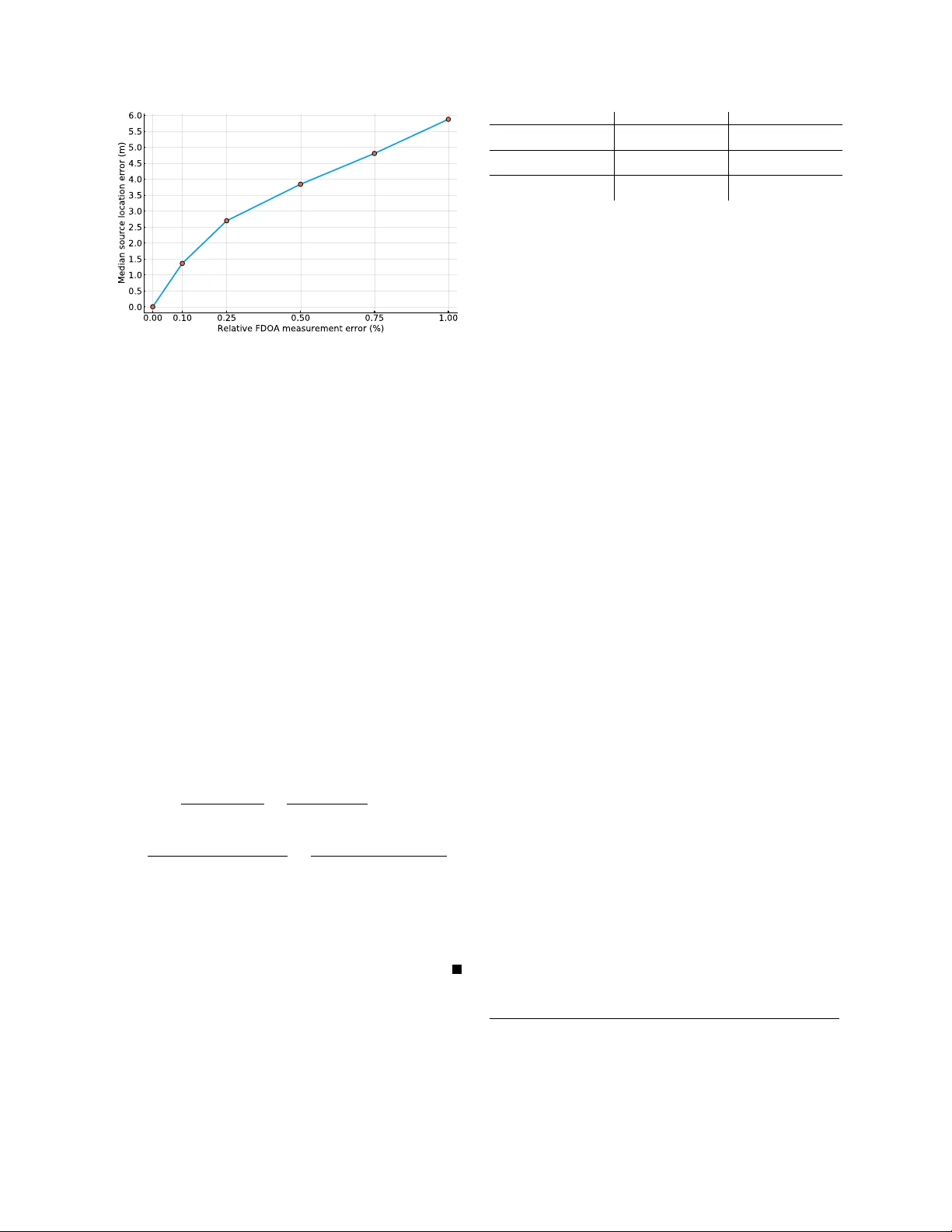
Geolocation with FDO A Measurements via Polynomial Systems and RANSA C Karleigh J. Cameron Dept. of Mathematics Colorado State Univ ersity Fort Collins, C0, 80523 (USA) Email: cameron@math.colostate.edu Daniel J. Bates Dept. of Mathematics Colorado State Univ ersity Fort Collins, C0, 80523 (USA) Email: bates@math.colostate.edu Abstract —The problem of geolocation of a transmitter via time difference of arriv al (TDO A) and frequency difference of arrival (FDOA) is given as a system of polynomial equations. This allows for the use of homotopy continuation-based methods from numerical algebraic ge- ometry . A novel geolocation algorithm employs numerical algebraic geometry techniques in conjunction with the random sample consensus (RANSA C) method. This is all developed and demonstrated in the setting of only FDO A measurements, without loss of generality . Additionally , the problem f ormulation as polynomial systems immediately pro vides lower bounds on the number of recei vers or measurements requir ed for the solution set to consist of only isolated points. I N T RO D U C T I O N The determination of the location of an RF transmitter based on measurements from sev eral receiv ers is a fundamental problem in a number of applications. These measurements include altitude (AL T), time difference of arriv al (TDO A), and frequency difference of arri val (FDOA) [11]. In fact, all of these measurements can be cast as polynomials in the v ariables corresponding to the location of the transmitter . The problem of geolocation can then be solved by computing numerical approximations of the solutions of polynomial systems, and it is simple to immediately provide lower bounds on the number of measurements needed to reduce the solution set dimension to zero (i.e., so there are only finitely many potential locations). Giv en a system of polynomial equations, the mathematical area called numerical algebraic geometry provides a range of tools and software for the solution of polynomial systems. Pairing this set of tools with the random sample consensus (RANSA C) method then yields a nov el approach to RF transmitter geolocation. The case of solving for emitter location using only TDO A measurements is simpler and has been well studied. Ho and Chan [11] provided a first dev elopment of equations for using TDOA measurements to back out emitter location, coming very close to the polynomial system dev elopment given in the next section. The more recent articles [7], [8] provide an advanced description of this TDOA-only setting, based largely on algebraic geometry . V arious other approaches have been de veloped, and at least one [14] has made use of numerical algebraic geometry , though in a rather different context. RANSA C has also pre viously been applied to the TDO A-only setting [12]. Although the methods dev eloped in this paper can be used to locate an emitter using TDOA measurements only , FDOA measurements only , or a combination of both, we choose to focus on the FDOA-only case. Doppler resolution is higher than range resolution for signals with narrow-bandwidth and long pulse duration [4], [13], making it desirable to solve for emitter location using FDO A alone in these cases. Source localization in the FDO A-only case, ho we ver , is far more nuanced, as the geometry associated with the FDOA measurements is more interesting and complicated [5]. For geolocation using FDO A alone in particular , there are often multiple possible emitter locations cor- responding to observed measurements. This can cause problems for iterativ e methods that conv erge to a single solution [13]. In contrast, numerical algebraic geometry techniques will find all real, feasible solutions. Our method then uses RANSA C to help determine which of these solutions is most consistent with other data gathered. In § I we formulate the TDOA- and FDO A-based source localization problem as polynomial systems and provide an introduction to methods from numerical algebraic geometry to be used for their solution. The proposed geolocation algorithm (FDOAR) incorporat- ing numerical algebraic geometry techniques and the iterativ e process, RANSAC, is presented in § II along with numerical results. A novel upper bound on fea- sible FDOA measurements for use in denoising data is presented in § III. In § IV we present lower bounds on the number of receivers or measurements needed to reduce the solution set to only isolated points. Benefits and limitations of the FDOAR geolocation algorithm are discussed in § V. The primary contributions of this article are • a dev elopment of the geolocation problem via TDO A and FDO A measurements as polynomial systems; • a novel upper bound on possible FDOA mea- surements; and • lower bounds on the number of receiv ers or measurements needed to reduce the solution set to only points; • a nov el approach to geolocation using the pairing of numerical algebraic geometry with RANSA C. I . B A C K G RO U N D A. P olynomial Systems for Geolocation Using a similar setup to that in [11], the relationship between TDOA measurements, FDOA measurements, and transmitter location can be represented as a set of polynomials. Consider a system of receivers, labeled 1 , . . . , N . W ithout loss of generality , the first receiver can be chosen as a reference receiv er , such that TDO A ( τ i, 1 ) and FDOA ( f i, 1 ) can be calculated between re- ceiv ers i and 1, where i = 2 , . . . , N , for a total of N − 1 pairs of measurements. The problem can be cast as two- or three- dimensional. For generality , we choose to use a three-dimensional earth-centered, earth fixed (ECEF) coordinate system. Thus, each receiver has known location x i = [ x i , y i , z i ] T and velocity ˙ x i = [ ˙ x i , ˙ y i , ˙ z i ] T . It is desirable to solve for the location of a radio-frequency emitter , x = [ x, y , z ] T . 1) T ime Dif fer ence of Arrival (TDO A): The amount of time it takes for the signal to travel from x to x i is k x − x i k /c , where c is the speed of propagation. Thus the TDOA between recei ver i and recei ver 1 is equiv alent to c · τ i, 1 = k x i − x k − k x 1 − x k = p ( x i − x ) 2 + ( y i − y ) 2 + ( z i − z ) 2 − p ( x 1 − x ) 2 + ( y 1 − y ) 2 + ( z 1 − z ) 2 . Considering all N receiv ers, this system can be trans- formed into the set of polynomial equations [11]: ( c · τ 1 , 2 ) 2 + 2 cr 1 · τ 1 , 2 − ( x 2 2 + y 2 2 + z 2 2 ) + ( x 2 1 + y 2 1 + z 2 1 ) + 2 [( x 2 − x 1 ) x + ( y 2 − y 1 ) y + ( z 2 − z 1 ) z ] = 0 ( c · τ 1 , 3 ) 2 + 2 cr 1 · τ 1 , 3 − ( x 2 3 + y 2 3 + z 2 3 ) + ( x 2 1 + y 2 1 + z 2 1 ) + 2 [( x 3 − x 1 ) x + ( y 3 − y 1 ) y + ( z 3 − z 1 ) z ] = 0 . . . ( c · τ 1 ,N ) 2 + 2 cr 1 · τ 1 ,N − ( x 2 N + y 2 N + z 2 N ) + ( x 2 1 + y 2 1 + z 2 1 ) + 2 [( x N − x 1 ) x + ( y N − y 1 ) y + ( z N − z 1 ) z ] = 0 r 2 1 − ( x 2 + y 2 + z 2 ) − ( x 2 1 + y 2 1 + z 2 1 ) + 2( x 1 x + y 1 y + z 1 z ) = 0 , where v ariable r 1 , representing the range of recei ver 1, is used to remov e square roots from the system. 2) F r equency Differ ence of Arrival (FDO A): As dev eloped in [11], the FDO A between receiv er i and receiv er 1 is, f i, 1 = f 0 c  ˙ x T i ( x i − x ) k x i − x k − ˙ x T 1 ( x 1 − x ) k x 1 − x k  , (1) where f 0 is the emitted frequency . Although more com- plicated than the TDO A case, the equations above can be conv erted to a polynomial system with the addition of more range variables, r i . The system becomes, r 1 r 2 f 1 , 2 − r 1 [ ˙ x 2 ( x 2 − x ) + ˙ y 2 ( y 2 − y ) + ˙ z 2 ( z 2 − z )] + r 2 [ ˙ x 1 ( x 1 − x ) + ˙ y 1 ( y 1 − y ) + ˙ z 1 ( z 1 − z )] = 0 r 1 r 3 f 1 , 3 − r 1 [ ˙ x 3 ( x 3 − x ) + ˙ y 3 ( y 3 − y ) + ˙ z 3 ( z 3 − z )] + r 3 [ ˙ x 1 ( x 1 − x ) + ˙ y 1 ( y 1 − y ) + ˙ z 1 ( z 1 − z )] = 0 . . . r 1 r N f 1 ,N − r 1 [ ˙ x N ( x N − x ) + ˙ y N ( y N − y ) + ˙ z N ( z N − z )] + r N [ ˙ x 1 ( x 1 − x ) + ˙ y 1 ( y 1 − y ) + ˙ z 1 ( z 1 − z )] = 0 r 2 1 − ( x 2 + y 2 + z 2 ) − ( x 2 1 + y 2 1 + z 2 1 ) + 2( x 1 x + y 1 y + z 1 z ) = 0 . . . r 2 N − ( x 2 + y 2 + z 2 ) − ( x 2 N + y 2 N + z 2 N ) + 2( x N x + y N y + z N z ) = 0 . 2 B. Numerical Methods for P olynomial Systems Rephrasing the above problems as systems of poly- nomial equations no w opens the door to methods from algebraic geometry , particularly numerical algebraic ge- ometry . The core computational engine of this field is homotopy continuation. The idea is as follo ws: Giv en a polynomial system of equations f ( z ) = 0 to be solved ( z ∈ C N ), a related system g ( z ) is constructed. For example, the total de gr ee start system for a system f ( z ) is given by g i ( z ) = z d i i − 1 , where d i is the degree of the polynomial f i ( z ) . A homotopy function, typically H ( z , t ) = t g ( z ) + (1 − t ) f ( z ) , between these two systems is then constructed so that H ( z , 1) = g ( z ) and H ( z , 0) = f ( z ) . Some basic algebraic geometry then guarantees that each isolated solution of f ( z ) = 0 will be reached by at least one path that v aries in t and includes a solution of g ( z ) = 0 . Thus, to find all isolated solutions of f ( z ) = 0 , it suf fices to find all solutions of g ( z ) and use numerical path-tracking methods [1] to mov e from t = 1 to t = 0 . Predictor-corrector methods are the standard choice. Extraneous paths will diver ge, but this wasted computation time can be partially mitigated by terminating any path with norm above some threshold or working in projecti ve space instead of af fine space. This is only a very basic description of a procedure that is fundamental in dozens of methods. For example, there are numerical methods for finding all complex positiv e-dimensional solution components (curves, sur- faces, etc.), for extracting real solutions in various circumstances, for making use of particular polynomial system structure to reduce run time, and so on. For man y further details, see [3], [15] and the references therein. For now , it suf fices to know a bit more about singular solutions, ill-conditioning, and parameter homotopies. 1) Singularity: Just as ( x − 1) 2 = 0 has a double root at x = 1 , isolated solutions of polynomial systems can hav e multiplicity greater than 1. The Jacobian matrix (the matrix of all first partial deriv ativ es of the system) is singular at such solutions, so these solutions are referred to as singular . The basic methods of numerical alge- braic geometry include so-called endgames , specialized techniques based on Puiseux series expansions or the Cauchy integral formula, which can be used to accu- rately compute numerical approximations to singular solutions of f ( z ) = 0 . Howe ver , when tracking paths before t = 0 , paths can become very close 1 , causing the Jacobian matrix to become ill-conditioned and resulting in poor path-tracking performance. This is mitigated in the software package Bertini [2] via step size control and adapti ve precision techniques, but can still lead to various recognizable tracking failures [3]. 1 Actual path crossing is a probability 0 event [3], [15]. 2) P arameter Homotopy: Finally , in the special set- ting of repeatedly solving polynomial systems with the same monomial structure but varying coefficients, there is a particular valuable tool called the parameter homotopy . The idea is as follo ws: Suppose we wish to find the solutions of a parameterized polynomial system of equations, f ( z ; p ) = 0 , at each of a large number n of parameter values p i ∈ P , i = 1 , . . . , n within some Euclidean (or possibly more general) parameter space P . W e could use the basic homotopy continuation mechanism described above, b ut there is a chance that much computational time will be wasted tracking (possibly many) di vergent paths for each p i . Instead, the idea of the parameter homotopy is to first solve f ( z ; p 0 ) for some random complex p 0 ∈ P , then start from only the finite solutions at p 0 to track to each p i . Once again, some basic algebraic geometry guarantees with probability 1 that the number of finite, isolated solutions at p = p 0 will be the maximum number of finite, isolated solutions at any choice of p . I I . N U M E R I C A L A L G E B R A I C G E O M E T RY A N D R A N S AC F O R F D OA - B A S E D G E O L O C A T I O N W ith a noiseless system, the numerical algebraic geometry methods above can be used to find all solu- tions to the FDO A system presented in § I-A2 accurate to any prescribed numerical accuracy . Specifically , it would take only a single solve in a software such as Bertini [2] to obtain an emitter location. Ho wev er , there are a couple issues that arise in real world situ- ations. First, noise and measurement error can plague FDO A calculations and recei ver location and velocity estimates. Additionally , if the recei vers are positioned in a singular configuration or near one, computing the solution may be prohibiti vely expensi ve and the solution itself could be much more accurate in some coordinates than in others. The nonlinear nature of the problem implies that there will often be multiple real solutions, which translate to multiple potential emitter locations. A robust accompaniment for the numerical algebraic ge- ometry methods above is an iterati ve process such as the RANdom SAmple Consensus (RANSA C) algorithm. RANSA C, originally developed [9] for application to the location determination problem, is useful when one has data with outliers or corrupt data points. The algorithm works by choosing a few samples from a set of data, determining a model to fit the samples, then calculating ho w man y of the remaining data points can be considered inliers with respect to that model, up to a predetermined tolerance. This process is repeated for a prescribed number of iterations, then the model with the most inliers is returned. As noted above, using RANSA C for geolocation is not a new idea. In fact, Li et al. applied the algorithm to source location with TDO A in [12]. This paper proposes 3 a modification of RANSA C to solve for source location with the FDO A polynomial system, a problem that is now accessible due to the utilization of numerical algebraic geometry techniques. The most notable benefit of using RANSA C for this problem is the ability to “ignore” noisy or corrupt data. Additionally , since many FDO A measurements are needed for the algorithm, it is natural to reformulate the polynomial system presented in § I-A2 to allow for measurements to be taken over multiple time steps. This reduces the number of receiv ers needed to a single pair, with each system composed of FDO A measurements from three separate time steps (see § IV for why data from three time steps is needed). The algorithm outlined below in v olves solving a sys- tem using the numerical algebraic geometry software, Bertini [2], during each iteration. Since each system will be of the same form and change only in certain parameter values (location, velocity , FDOA measure- ments), the solve can be structured as a parameter homo- topy [3], [15]. As discussed in § I-B, this allows for only necessary paths to be tracked, which provides faster run times. Additionally , when the solving of an FDOA system results in multiple real, feasible solutions, we hav e modified the algorithm to consider each solution separately . This ensures there are no missed solutions, as can often result from iterative geolocation methods that con ver ge to a single solution [13]. A. FDO A-RANSA C (FDO AR) Algorithm Outline Input : • Locations, velocities, and corresponding FDO A measurement ( f i ) for n pairs of receiv ers (or n timesteps of 1 pair of receiv ers). • Number of iterations to run algorithm ( maxiter ). • Inlier tolerance ( ε ). Output : • Estimated transmitter location, x . 1) Select three sample points from receiver data (FDOA measurements, receiver loca- tions and velocities). 2) Solve for emitter location using Bertini. 3) Determine feasible solutions (must have positiv e range values and satisfy Prop. III.1). 4) For each feasible solution, determine the number of sample pairs that can be con- sidered inliers. a) For each pair of recei vers, deter - mine the theoretical FDO A mea- surement, ˆ f i , corresponding to the solution. • If | ˆ f i − f i | < ε , mark sample as an inlier . b) If the number of inliers for the current solution is greater than the pre vious recorded location, record current solution as best source location estimate. 5) Repeat for designated number of iterations and return transmitter location estimate. B. Numerical P erformance Numerical simulations were run as follows. Con- sider a Cartesian cube of space, 100m long on each side. For each numerical trial, a transmitter was placed at a random location, x , in the cube. Locations and velocities for 40 pairs of receivers were also generated, with locations being limited to the interior of the cube and velocities in the range [ − 2 , 2] m/s in each (x,y ,z) direction. This is meant to simulate 40 time steps for a single pair of receiv ers and a stationary transmitter . For each pair of receiv ers, the FDOA was calculated according to Eq. 1 and noise was added to simulate various lev els of relati ve FDOA measurement error . W e define this, Relativ e FDOA Measurement Error := σ 2 noise σ 2 F DO A × 100% , where σ 2 noise and σ 2 F DO A are the variance of the noise and variance of observed FDOA, respecti vely . The FDO AR algorithm was then run for 20 iterations, returning final transmitter estimate ˆ x . The error for the trial was then calculated: k ˆ x − x k (m). Results are sho wn in Fig. 1. For each data point, this process was repeated 50 times and the median of the error was recorded. Many of the worst performing trials above resulted from transmitters located near the edges of the Cartesian box. W e hypothesize that this is the result of very few (or none) of the receiv er pairs being located on the side of the transmitter closest to the edge of the box. This caused less information to be learned about the transmitter and resulted in a worse estimate. This is consistent with geolocation intuition and suggests that error v alues in Fig. 1 w ould decrease if one could ensure that receiv ers view the emitter from a v ariety of angles. 4 Fig. 1: Error in emitter location resulting from various lev els of FDO A measurement error . For each data point, 50 instances of coupled RANSA C and Bertini were run, each having 20 iterations and ε = 0 . 03 . I I I . N OT E O N D E N O I S I N G Since one of the key contributions of this article is the use of RANSAC for denoising data, we include here a brief result that allows us to immediately remove FDO A measurements that are physically unrealizable due to measurement error or noise. Proposition III.1. The frequency differ ence of arrival between r eceivers i and j , f i,j satisfies: | f i,j | ≤ k v j k + k v i k , wher e v i and v j ar e the velocity vectors of receivers i and j , r espectively . Pr oof: | f i,j | =     v j · ( x j − x ) k x j − x k − v i · ( x i − x ) k x i − x k     =     k v j kk x j − x k cos( θ j ) k x j − x k − k v i kk x i − x k cos( θ i ) k x i − x k     = |k v j k cos( θ j ) − k v i k cos( θ i ) | ≤ k v j k + k v i k . It would also be interesting to consider denoising via projection to the manifold of realizable FDO A measurements, similar to the use of projection in linear regression. A similar approach was pre viously taken in the TDO A case [6]. W e leav e this for future work. # measurements (2D) # measurements (3D) TDOA only 2 3 TDOA + AL T - 2 FDOA only 2 3 FDOA + AL T - 2 TDOA + FDOA 1 2 TDOA + FDOA + AL T - 1 T ABLE I: Minimum number of TDOA and FDO A mea- surements necessary to reduce set of potential transmit- ter locations to a finite number , for v arying dimensions (2 or 3) and types of measurements being used. I V . B O U N D S O N T H E N E C E S S A RY N U M B E R O F M E A S U R E M E N T S For systems of linear equations, it is tri vial to predict the dimension of the solution set under the assumption that the equations are linearly independent. This is much the same with polynomial systems, though the range of degenerate cases is far more nuanced and complicated. W ith the formulation of the geolocation problem as a system of polynomial equations in § I-A, it is easy to provide bounds on the minimum number of TDO A and FDO A measurements 2 needed in various scenarios to reduce the solution set to a finite set of points. The case is also considered where altitude of the emitter is known (AL T constraint). This is the content of T able 1. It is important to note that these bounds do not guarantee that there will be only finitely many solutions for every set of measurements. As an extreme coun- terexample, consider the case of stacking all receiv ers at the same point; the number of (identical) measurements in this case makes no dif ference. It is also worth noting that an anomalous positive- dimensional component (with r 1 = 0 ) shows up in the FDO A only case. Howe ver , this component is easily ignored as it is not physically feasible. V . D I S C U S S I O N A. Benefits of FDO AR W e summarize a few of the primary benefits of our approach here: 1) Solving the geolocation systems using nu- merical algebraic geometry techniques finds all possible emitter locations. Coupling with RANSA C provides a w ay to determine which 2 If we do not allow receivers to take measurements over multiple time steps, a similar table could be provided showing bounds on the number of receiv ers necessary . Here we refer to the number of measurements rather than the number of receivers for generality . 5 one of those locations best matches the rest of the data. 2) Any bad data from path failures, inaccuracies, measurement error , etc. is automatically ig- nored, assuming the source of the errors is not implicit in the structure of the problem. 3) Our method uses FDO A measurements only , though it can be adapted to other measurement combinations. 4) Using multiple time steps, it is necessary to use only two receivers. Additionally , there is no need to designate a reference recei ver , which could corrupt all data points if there are errors in its location or velocity . 5) When performing polynomial system solves at multiple points in parameter space, parameter homotopies could improv e efficienc y . B. Limitations Each path tracked when solving a polynomial sys- tem requires dozens, sometimes hundreds, of linear solves. As a result, any polynomial systems approach will necessarily be slower than any linear approach. Howe ver , linearization necessarily introduces inaccu- racy to nonlinear problems, so the trade-off between speed and accuracy might lead different users to use different approaches. As with any RANSA C implementation, speed and accuracy is in part dependent upon the users choice of the maximum number of iterations and inlier tolerance. The optimal choice for these variables can depend greatly on the specifics of the problem. Theoretical re- sults exist that bound the maximum number of iterations with respect to the percentage of inliers present in the data [16]. V I . F U T U R E W O R K The problem of transmitter geolocation is mathemat- ically rich and practically valuable. As a result, there are many potential a venues worthy of consideration. Giv en a configuration of receiv ers and a generic set of measurements, it should be possible to decompose the space of emitter locations into chambers corresponding to the number of physically realizable solutions of the corresponding geolocation polynomial system. An analysis over some set of such configurations could then help in choosing “good” receiv er configurations. Simi- larly , methods such as gradient descent homotopies [10] could be useful in finding the boundaries (called the discriminant locus ) between these chambers. As described abov e, it would be interesting to under- stand and make use of the semialgebraic set of physi- cally realizable FDOA measurements (see § III). Perhaps this would provide some intuition for the estimation of geolocation accuracy . A C K N O W L E D G M E N T S Both authors were partially supported by NSF grant DMS–1719658 and AFOSR grant F A9550-14-1-0185. The authors wish to thank the PI of that AFOSR grant, Margaret Cheney , for introducing us to this problem and numerous stimulating discussions. W e also wish to thank Jon Hauenstein for suggesting the use of RANSA C. R E F E R E N C E S [1] E. L. Allgower and K. Georg. Intr oduction to Numerical Continuation Methods . SIAM, Philadelphia, 2003. [2] D. Bates, J. Hauenstein, A. Sommese, and C. W ampler . Bertini: Software for numerical algebraic geometry . A v ailable at be- tini.nd.edu. [3] D. Bates, J. Hauenstein, A. Sommese, and C. W ampler . Bertini: Softwar e for numerical algebraic geometry . 2015. [4] M. Cheney and B. Borden. Fundamentals of Radar Imaging . Society for Industrial and Applied Mathematics, 2009. [5] M. Cheney and J. A. Given. W ideband passi ve source local- ization. Inverse Problems , 33(8):085007, 2017. [6] M. Compagnoni, A. Canclini, P . Bestagini, F . Antonacci, A. Sarti, and S. T ubaro. Source localization and denoising: a perspectiv e from the TDOA space. Multidimensional Systems and Signal Pr ocessing , 28(4):1283–1308, Oct 2017. [7] M. Compagnoni, R. Notari, F . Antonacci, and A. Sarti. A comprehensiv e analysis of the geometry of TDOA maps in localization problems. Inverse Problems , 30(3), 2014. [8] M. Compagnoni, R. Notari, A. A. Ruggiu, F . Antonacci, and A. Sarti. The algebro-geometric study of range maps. arXiv:1604.08076 , 2016. [9] M. A. Fischler and R. C. Bolles. Random sample consensus: A paradigm for model fitting with applications to image analysis and automated cartography . Commun. A CM , 24(6):381–395, June 1981. [10] Z. Griffin and J. Hauenstein. Real solutions to systems of polynomial equations and parameter continuation. Advances in Geometry , 15(2):173–187, Apr . 2015. [11] K. C. Ho and Y . T . Chan. Geolocation of a known altitude object from TDO A and FDOA measurements. IEEE T rans- actions on Aer ospace and Electr onic Systems , 33(3):770–783, July 1997. [12] P . Li and X. Ma. Robust Acoustic Sour ce Localization with TDO A Based RANSAC Algorithm , pages 222–227. Springer Berlin Heidelberg, Berlin, Heidelberg, 2009. [13] J. Mason and L. Romero. T oa/foa geolocation solutions using multiv ariate resultants. Navigation , 52(3):163–177, 2005. [14] S. Shuster, A. J. Sinclair, and T . A. Lov ell. Initial relative- orbit determination using heterogeneous TDO A. In 2017 IEEE Aer ospace Conference , pages 1–7, March 2017. [15] A. Sommese and C. W ampler . Numerical solution of poly- nomial systems arising in engineering and science . W orld Scientific, Singapore, 2005. [16] T . Urban ˘ ci ˘ c, M. Fras, B. Stopar, and K. Bo ˘ zo. The influence of the input parameters selection on the RANSA C results. 13:159– 170, 06 2014. 6