Event-Triggered Algorithms for Leader-Follower Consensus of Networked Euler-Lagrange Agents

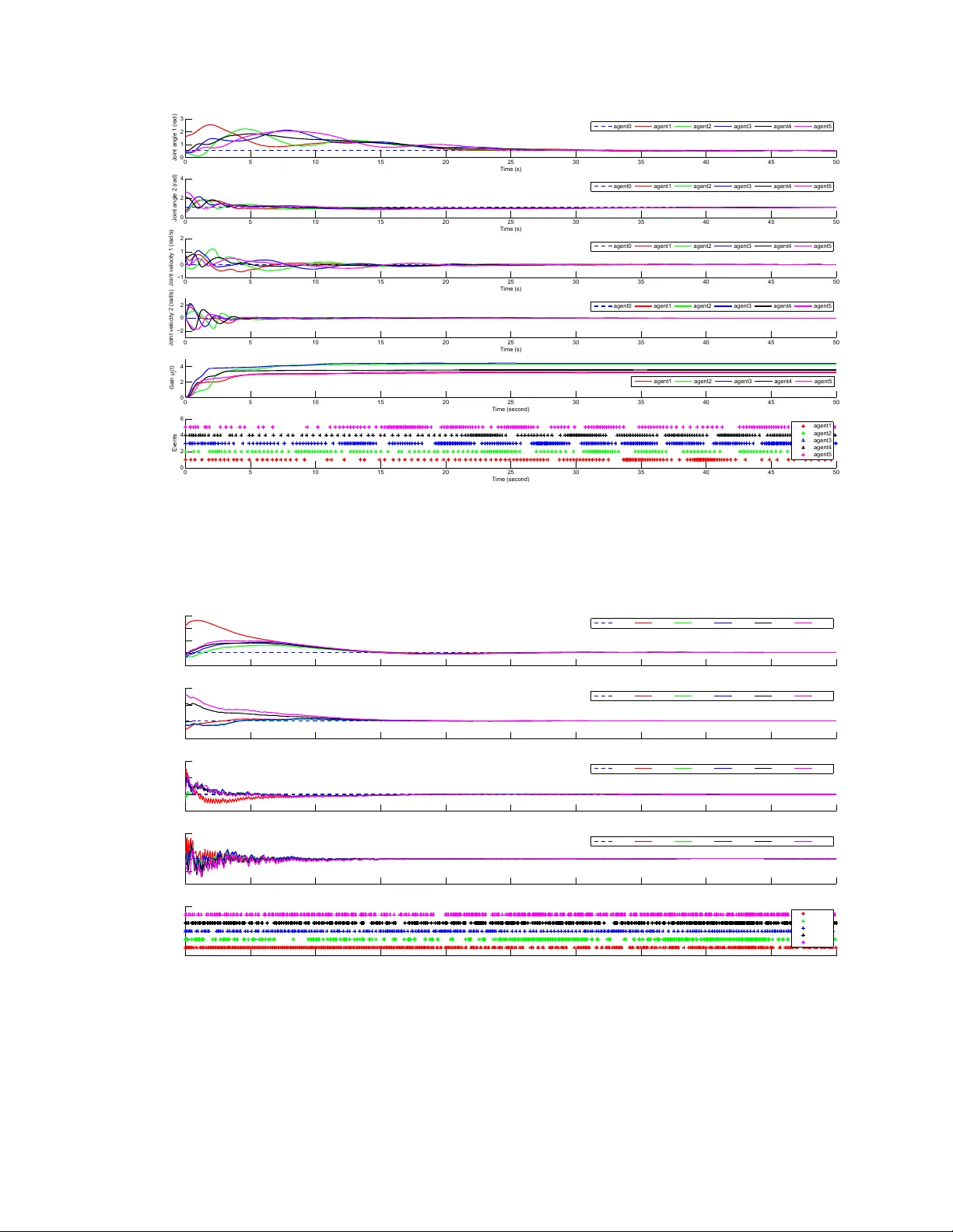
1 Ev ent-T riggered Algorithms for Leader -F ollo wer Consensus of Network ed Euler -Lagrange Agents Qingchen Liu, Mengbin Y e, Jiahu Qin and Changbin Y u Abstract —This paper proposes thr ee different distrib uted event-trigger ed control algorithms to achiev e leader-f ollower consensus for a netw ork of Euler -Lagrange agents. W e ﬁrstly propose two model-independent algorithms for a subclass of Euler -Lagrange agents without the vector of gravitational po- tential f orces. By model-independent, we mean that each agent can execute its algorithm with no knowledge of the agent self- dynamics. A v ariable-gain algorithm is employed when the sensing graph is undirected; algorithm parameters are selected in a fully distributed manner with much gr eater ﬂexibility com- pared to all pre vious work concerning ev ent-triggered consensus problems. When the sensing graph is directed, a constant-gain algorithm is employed. The control gains must be centrally designed to exceed several lower bounding inequalities which requir e limited knowledge of bounds on the matrices describing the agent dynamics, bounds on network topology inf ormation and bounds on the initial conditions. When the Euler -Lagrange agents hav e dynamics which include the vector of gravitational potential for ces, an adaptive algorithm is proposed which requir es more information about the agent dynamics but can estimate uncertain agent parameters. For each algorithm, a trigger function is proposed to gover n the ev ent update times. At each event, the controller is updated, which ensures that the control input is piecewise constant and sav es energy resour ces. W e analyse each controllers and trigger function and exclude Zeno behaviour . Extensive simulations show 1) the advantages of our proposed trigger function as compared to those in existing literature, and 2) the effectiveness of our proposed controllers. I . I N T RO D U C T I O N The ﬁeld of multi-agent systems has recei ved extensiv e attention from the control community in the past two decades. In particular, coordination of a network of interacting agents to achieve a global objectiv e has been seen as a key sub-area within the ﬁeld. See [1] for a recent survey . Leader-follo wer consensus is a variation of the commonly studied consensus problem where, with all agents having a commonly deﬁned state variable(s), the network of follower agents con ver ge to the state v alues of the stationary leader . This is achie ved by interaction between neighbouring agents. By the fact that interaction is only between neighbouring agents then each follower agent must use a distributed controller, i.e. agents cannot use global information about the whole network [2]. The Euler-Lagrange equations describe the dynamics of a large class of nonlinear systems (including many mechan- Q. Liu, M. Y e and C. Y u are with the Research School of Engi- neering, Australian National University , Canberra A CT 0200, Australia. C. Y u is also with the School of Automation, Hangzhou Dianzi Univer- sity , Hangzhou 310018, China. { qingchen.liu, mengbin.ye, brad.yu } @anu.edu.au . J. Qin is with the Department of Automation, Univ ersity of Science and T echnology of China, Hefei 230027, China. jhqin@ustc.edu.cn ical systems such as robotic manipulators, spacecraft and marine vessels) [3], [4]. As a result, there is motiv ation to study multi-agent coordination problems where each agent has Euler-Lagrange dynamics [5]. Leader-follo wer consensus for directed networks of Euler-Lagrange agents has been studied in [6] using a model-independent controller , and in [7] using an adaptiv e controller . In both, the topology requires a directed spanning tree. Recently , use of ev ent-triggered controllers has been popu- larised in multi-agent coordination problems [8]. While each agent has continuous time dynamics, the controller is updated at discrete time instants based on ev ent-scheduling. Because the controller updates occur at speciﬁc ev ents, this has the beneﬁt of reducing actuator updates. Howe ver , it is important to properly design and analyse the e vent-scheduling trigger function to exclude Zeno behaviour [9], [10], which can cause the controller to collapse. Numerous results have been published studying consensus based problems using distrib uted ev ent-triggered control laws. Howe v er , the majority study agents with single and double-integrator dynamics [11]–[16]. There hav e been relati vely fe w results published studying ev ent-triggered control for networks of Euler-Lagrange agents. Pioneering contributions studied leaderless consensus (b ut not leader-follo wer consensus) on an undirected network [17], [18]. The dynamics studied in [17] and [18] are a subclass of Euler-Lagrange dynamics as they do not consider the pres- ence of gravitational forces for each agent. While continuous model-independent algorithms e.g. [6] are easily adapted to be ev ent-triggered, as shown in [17], [18], they cannot guarantee the coordination objectiv e in the presence of gravitational forces (which has an ef fect which is similar to a bounded disturbance). T ypical control techniques required to deal with this term include feedback linearisation [19], adaptiv e con- trol [7] and sliding mode control [20]. W e note that these techniques have not been well studied in an ev ent-triggered framew ork. In fact, ﬁrst-order sliding mode controllers exhibit Zeno-like beha viour and thus are unsuitable for implemen- tation in ev ent-triggered control. In [21], an adaptive, event- triggered controller is proposed to achieve ﬂocking behaviour for undirected networks of Euler-Lagrange agents. This allows for gravitational forces omitted in [17], [18]. Howe ver , the proposed controller is piecewise continuous, which restricts its implementation in digital platforms. Moreover , it is worth noting that the trigger function used in [21] cannot eliminate Zeno beha viour for each agent. 2 A. Contributions of This P aper In this paper , we propose three different distributed ev ent- triggered control algorithms to achie ve leader-follo wer con- sensus for networked Euler-Lagrange agents; each algorithm has different strengths and their appropriateness of use may depend on the application scenario. W e propose two model-independent controllers for Euler- Lagrange agents without the gravitational term (unlike the model-dependent algorithm in [17]). Firstly , a globally asymp- totically stable v ariable-gain model-independent algorithm is proposed for agents on undirected graphs. The v ariable-gain controller allows for fully distributed and arbitrary design of parameters in both the control algorithm and trigger function . F or agents with complex dynamics, almost all existing results r equir e centralised design of key parameters in the trigger function using limited global knowledge of the network [17], [21], [22]. The design of these key parameter s is to ensure either Zeno-fr ee behaviour , or to guarantee con ver gence of the contr oller . In the case of simple agent dynamics, the pa- rameters are distributed in design but must either obe y upper or lower bounds [11]–[13], [23]. As such, the fully distributed variable-g ain controller represents a signiﬁcant adv ance on existing event-triggered control algorithms, because stability and con ver gence are always guaranteed, e ven if the algorithm and trigger function parameters are arbitrarily selected. Even when implemented continuously , and with simple agent dynamics, variable-gain algorithms on directed graphs are difﬁcult to analyse [24]–[26]. For the second model- independent controller , which is applicable for directed graphs, we are therefore moti v ated to use constant control gains. It will become apparent in the sequel that, e ven when the controller has constant gains, the combination of Euler-Lagrange dynam- ics, directed topology , and event-based control requires non- triv al stability analysis. The algorithm achieves leader -follo wer consensus semi-globally , exponentially fast (neither directed graphs nor e xponential stability has not been established in an y existing results on ev ent-based networks of Euler -Lagrange agents). Some limited knowledge of the bounds on the agent dynamic parameters, the network topology and a set of all possible initial conditions is required to centrally design the control gains. This is a trade-off for allowing agents to interact on a directed graph. Lastly , we propose a globally asymptotically stable adaptiv e algorithm for use when the gravitational term is present in the agent self-dynamics; this algorithm appeared in our preliminary work [27]. The adaptiv e algorithm is able to es- timate uncertain dynamical parameters, but requires increased knowledge about the agent self-dynamics. All three proposed controllers are piece wise constant (unlike the piecewise continuous algorithm in [21]), which has the beneﬁt of reducing actuator updates and thus conserving energy resources. Furthermore, each agent only requires state, and relati ve state measurements, and does not require knowl- edge of the trigger times of neighbouring agents (unlike [17], [21]). For each algorithm, a trigger function is proposed and we show that Zeno beha viour can be excluded for e very agent by pro ving that for any ﬁnite interv al of time, a strictly positiv e lower bound exists on the time between each ev ent. All three trigger functions are of the same form with only minor modiﬁcations. Each term of the trigger function is carefully selected to ensure that the trigger function is more effecti v e, when compared with existing trigger functions which do one or the other , at 1) reducing the total number of ev ents, and 2) eliminating Zeno behaviour for ev ery agent. W e show this by detailed comparison and analysis based on simulations. As a result of having multiple terms in the trigger function to achieve the aforementioned improvements, the stability analysis is made signiﬁcantly more complicated. Each algorithm requires a different approach to proving stability , and the proposed methods may be useful for other problems in e vent-based control of multi-agent systems. B. Structure of the Rest of the P aper Section II provides mathematical notations and background on graph theory and Euler -Lagrange systems. A formal prob- lem deﬁnition is also provided. The three different distributed ev ent-triggered control algorithms are then proposed and anal- ysed in Section III, IV and V, separately . Simulations in Section VI show the effecti veness of the proposed controllers. Concluding remarks are giv en in Section VII. I I . B A C K G RO U N D A N D P R O B L E M S T A T E M E N T A. Notations and Mathematical Pr eliminaries In this paper , R n denotes the n -dimensional Euclidean space and R m × n denotes the set of m × n real matrices. The transpose of a vector or matrix A is giv en by A > . The i th smallest eigen value of a symmetric matrix A is denoted by λ i ( A ) . Let x = [ x 1 , . . . , x n ] > where x i ∈ R n × n and n ≥ 1 . Then diag { x } denotes a (block) diagonal matrix with the (block) elements of x on its diagonal, i.e. diag { x 1 , ..., x n } . A symmetric matrix A ∈ R n × n which is positiv e deﬁnite (respectiv ely nonnegativ e deﬁnite) is denoted by A > 0 (respectiv ely A ≥ 0 ). For two symmetric matrices A , B , the expression A > B is equiv alent to A − B > 0 . The n × n identity matrix is I n and 1 n denotes an n -tuple column vector of all ones. The n × 1 column vector of all zeros is denoted by 0 n . The symbol ⊗ denotes the Kronecker product. The Euclidean norm of a vector , and the matrix norm induced by the Euclidean norm, are denoted by k · k . The absolute value of a real number is | · | . For the space of piecewise continuous, bounded vector functions, the norm is deﬁned as k f k L ∞ = sup k f ( t ) k < ∞ and the space is denoted by L ∞ . The space L p for 1 ≤ p < ∞ is deﬁned as the set of all piecewise continuous vector functions such that k f k L p =  R ∞ 0 k f ( t ) k p dt  1 /p < ∞ where p refers to the type of p -norm. Sev eral theorems, lemmas and corollaries are now intro- duced, which will be used in this paper . Theorem 1 (Mean V alue Theorem for V ector-V alued Func- tions [28]) . F or a continuous vector-valued function f ( s ) : R → R n differ entiable on s ∈ [ a, b ] , ther e exists t ∈ ( a, b ) such that     d f ds ( t )     ≥ 1 b − a k f ( b ) − f ( a ) k 3 Theorem 2 (The Schur Complement [29]) . Consider a sym- metric bloc k matrix, partitioned as A =  B C C > D  (1) Then A > 0 if and only if B > 0 and D − C > B − 1 C > 0 . Equivalently , A > 0 if and only if D > 0 and B − C D − 1 C > > 0 . Lemma 1. (F r om [30]) If a function f ( t ) satisﬁes f ( t ) , ˙ f ( t ) ∈ L ∞ , and f ( t ) ∈ L p for some value of p ∈ [1 , ∞ ) , then f ( t ) → 0 as t → ∞ . Lemma 2. Suppose A > 0 is deﬁned as in (1) . Let a quadratic function with ar guments x , y be expr essed as W = [ x > , y > ] A [ x > , y > ] > . Deﬁne F := B − C D − 1 C > and G := D − C > B − 1 C . Then ther e holds λ min ( F ) x > x ≤ x > F x ≤ W (2a) λ min ( G ) y > y ≤ y > Gy ≤ W (2b) Pr oof. The proof for (2b) is immediately obtained by recalling Theorem 2 and observing that W = y > Gy + [ y > C > B − 1 + x > ] B [ B − 1 C y + x ] An equally straightforward proof yields (2a). Lemma 3. Let g ( x, y ) be a function given as g ( x, y ) = ax 2 + by 2 − cxy 2 − dxy (3) for r eal positive scalars a, c, d > 0 . Then for a given X > 0 , ther e exist b > 0 suc h that g ( x, y ) > 0 for all y ∈ [0 , ∞ ) and x ∈ [0 , X ] . Pr oof. See Appendix A. Corollary 1. Let h ( x, y ) be a function given as h ( x, y ) = ax 2 + by 2 − cxy 2 − dxy − ex − f y (4) wher e the real, strictly positive scalars c, d, e, f and two further positive scalars ε, ϑ are ﬁxed. Suppose that for given Y , ε ther e holds Y − ε > 0 , and for a given X > 0 there holds X − ϑ > 0 . Deﬁne the sets U = { x, y : x ∈ [ X − ϑ, X ] , y > 0 } and V = { x, y : x > 0 , y ∈ [ Y − ε, Y ] } . Deﬁne the r e gion R = U ∪ V . Then ther e e xist a, b > 0 such that h ( x, y ) is positive deﬁnite in R . Pr oof. See Appendix A. B. Graph Theory W e model the interactions among the leader and n followers by a weighted directed graph (digraph) G = ( V , E , A ) with verte x set V = { v 0 , v 1 , · · · , v n } and edge set E ⊆ V × V . W ithout loss of generality , the leader agent is numbered by v 0 . W e use G F to describe the interactions among the n follower agents with vertex set V F = { v 1 , · · · , v n } and edge set E F ⊆ V F × V F . An ordered edge set of G is e ij = ( v i , v j ) . The weighted adjacency matrix A = A ( G ) = { a ij } is the ( n + 1) × ( n + 1) matrix gi ven by a ij > 0 , if e j i ∈ E and a ij = 0 , otherwise. In this paper , it is assumed that a ii = 0 , i.e. there are no self-loops. The edge e ij is incoming with respect to v j and outgoing with respect to v i . A graph is undirected if e ij ∈ E ⇔ e j i ∈ E and a ij = a j i . The neighbour set of v i is denoted by N i = { v j ∈ V : ( v i , v j ) ∈ E } . The ( n + 1) × ( n + 1) Laplacian matrix, L = { l ij } , of the associated directed graph G is deﬁned as l ij = ( P n k =1 ,k 6 = i a ik for j = i − a ij for j 6 = i A digraph with n + 1 vertices is called a directed spanning tree if it has n edges and there exists a root vertex with directed paths to ev ery other verte x [2]. The following result holds for the Laplacian matrix associated with a directed graph. Lemma 4. (F r om [2]) Let L be the Laplacian matrix as- sociated with a directed graph. Then L has a simple zer o eigen value and all other eigen values have positive real parts if and only if G has a directed spanning tr ee. Lemma 5. (F r om [31]) Suppose a gr aph G contains a dir ected spanning tr ee, and there ar e no edges of G which are incoming to the r oot vertex v 0 of the tr ee. Then the Laplacian matrix associated with G has the following form: L =  0 0 T n − 1 L 21 L 22  and all eigen values of L 22 have positive r eal parts. Mor eover , ther e exists a diagonal positive deﬁnite matrix Γ such that Q := Γ L 22 + L > 22 Γ > 0 . In addition, if G F is undir ected, then L 22 is symmetric positive deﬁnite. C. Euler-Lagr ange Systems A class of dynamical systems can be described using the Euler-Lagrange equations [3]. The general form for the i th agent equation of motion is: M i ( q i ) ¨ q i + C i ( q i , ˙ q i ) ˙ q i + g i ( q i ) = τ i (5) where q i ∈ R p is a vector of the generalized coordinates, M i ( q i ) ∈ R p × p is the inertial matrix, C i ( q i , ˙ q i ) ∈ R p × p is the Coriolis and centrifugal torque matrix, g i ( q i ) ∈ R p is the vector of gravitational forces and τ i ∈ R p is the control input vector . For agent i , we hav e q i = [ q (1) i , . . . , q ( p ) i ] > . W e assume each agent is fully actuated. The dynamics in (5) are assumed to satisfy the following properties, details of which are provided in [3]. P1 The matrix M i ( q i ) is symmetric positiv e deﬁnite. P2 There exist constants k m , k M > 0 such that k m I p ≤ M i ( q i ) ≤ k M I p , ∀ i, q i . It follo ws that sup q i k M i k 2 ≤ k M and k m ≤ inf q i k M − 1 i k 2 − 1 ∀ i . P3 There exists a constant k C > 0 such that k C i k 2 ≤ k C k ˙ q i k 2 , ∀ i, ˙ q i . P4 The matrix C i ( q i , ˙ q i ) is related to the inertial ma- trix M i ( q i , ˙ q i ) by the expression x T ( 1 2 ˙ M i ( q i ) − C i ( q i , ˙ q i )) x = 0 for any q , ˙ q , x ∈ R p . This implies that ˙ M i ( q i ) = C i ( q i , ˙ q i ) + C i ( q i , ˙ q i ) > . P5 There exists a constant k g > 0 such that k g i ( q i ) k < k g . P6 Linearity in the parameters: M i ( q i ) x + C i ( q i , ˙ q i ) y + g i ( q i ) = Y i ( q i , ˙ q i , x , y ) Θ i for all vectors x, y ∈ R p , 4 where Y i ( q i , ˙ q i , x , y ) is the kno wn regressor matrix and Θ i is a vector of unknown but constant parameters associated with the i th agent. Remark 1. It is assumed thr oughout this paper that the pr operties P1 thr ough to P6 always hold. Assumption 1 (Sub-class of dynamics) . In Sections III and IV, we assume that g i ( q i ) = 0 , ∀ i . In other words, the dynamics of the a gents belong to a subclass of Euler -Lagrang e equations which do not have a gravity term. That is, M i ( q i ) ¨ q i + C i ( q i , ˙ q i ) ˙ q i = τ i (6) If the gravity term g i ( q i ) is present, the adapti ve controller proposed in Section V may be used. D. Pr oblem Statement Denote the leader as agent 0 with q 0 and ˙ q 0 being the generalised coordinates and generalised velocity of the leader , respectiv ely . The aim is to de velop event-based, distributed algorithms for each Euler -Lagrange follower agent, where the updates are such that τ i is piece wise-constant. The distributed algorithms are designed to achieve leader-follower consensus to a stationary leader , i.e. ˙ q 0 ( t ) = 0 , ∀ t ≥ 0 . Leader-follo wer consensus is said to be achieved if lim t →∞ k q i ( t ) − q 0 ( t ) k = 0 , ∀ i = 1 , . . . , n and lim t →∞ k ˙ q i ( t ) k = 0 , ∀ i = 1 , . . . , n are satisﬁed. Another aim of this paper is to exclude the possibility of Zeno behaviour . W e provide a formal deﬁnition of Zeno behaviour in the sequel. Zeno behaviour of an e vent-based controller means an inﬁnite number of controller updates occur in a ﬁnite time period, which is undesirable since no practical controller can do this. In this paper , we assume that agent i ∈ 1 , . . . , n is equipped with sensors which continuously measures the relati ve gen- eralised coordinates to agent i ’ s neighbours. In other words, q i ( t ) − q j ( t ) , ∀ j ∈ N i is av ailable to agent i . In Section IV we also assume that the relati ve generalised velocities are av ailable, i.e. ˙ q i ( t ) − ˙ q j ( t ) , ∀ j ∈ N i . The scenario where agents collect relati ve information to execute algorithms can be found in many experimental testbeds, such as ground robots or U A Vs equipped with high-speed cameras. It is also assumed that each agent i can measure its own generalised velocity continuously , ˙ q i ( t ) . Deﬁnition 1. Let a ﬁnite time interval be t Z = [ a, b ] where 0 ≤ a < b < ∞ . If, for some ﬁnite k ≥ 0 , the sequence of event triggers { t i k , ..., t i ∞ } ∈ [ a, b ] then the system exhibits Zeno behaviour . I I I . M A I N R E S U LT : A V A R I A B L E - G A I N , M O D E L - I N D E P E N D E N T C O N T RO L L E R O N U N D I R E C T E D N E T W O R K S In this section, we introduce a variable gain, ev ent-triggered control algorithm to achie ve leader-follo wer consensus for Euler-lagrange agents where the network model of the follower agents is described by an undirected network. W e show that the proposed algorithm do not require any kno wledge of the multi- agent system (i.e totally distributed design) and is globally stable. Zeno beha viour is also excluded for each agent in the system. A. Main Result Deﬁne a new state variable for agent i as z i ( t ) = n X j =0 a ij ( q i ( t ) − q j ( t )) + µ i ( t ) ˙ q i ( t ) , i = 1 , . . . , n where a ij is an element of the adjacency matrix A associated with the digraph G . Note that the follower graph G F is undirected. W e let µ i ( t ) be subject to the follo wing updating law: ˙ µ i ( t ) = α ˙ q > i ( t ) ˙ q i ( t ) (7) The scalar α is strictly positiv e and is univ ersal for all agents. It is obvious that µ i ( t ) is a monotonically increasing function. The variable-gain scalar function µ i ( t ) is initialised at t = 0 with an arbitrary µ i (0) ≥ 0 , which implies that µ i ( t ) ≥ 0 , ∀ t > 0 . The control algorithm is no w proposed. Let the trigger time sequence of agent i be t i 0 , t i 1 , . . . , t i k , . . . with t i 0 := 0 and we detail belo w ho w each trigger time is determined. The e vent- triggered controller for follower agent i is designed as: τ i ( t ) = − z i ( t i k ) (8) for t ∈ [ t i k , t i k +1 ) . The control input for each agent is held constant and equal to the last control update τ i ( t i k ) in the time interv al [ t i k , t i k +1 ) . W e deﬁne a state mismatch for agent i between consecutive ev ent times t i k and t i k +1 as follo ws: e i ( t ) = z i ( t i k ) − z i ( t ) (9) for t ∈ [ t i k , t i k +1 ) . Then we design the trigger function as follows: f i ( e i , ˙ q i , ω i ) = k e i ( t ) k 2 − β i k ˙ q i ( t ) k 2 − ω i ( t ) (10) where β i is an arbitrarily chosen positive constant (see the Proof of Theorem 3 for the explanations), ω i ( t ) is an offset function deﬁned as ω i ( t ) = κ i exp( − ε i t ) with arbitrarily chosen κ i , ε i > 0 . The k th ev ent for agent i is triggered as soon as the trigger condition f i ( e i , ˙ q i , ω i ) = 0 is satisﬁed. The control input τ i ( t ) is updated only when an event of agent i is triggered. Furthermore, ev ery time an ev ent is triggered, and in accordance with their deﬁnitions, the measurement error e i ( t ) is reset to be equal to zero and thus the trigger function assumes a non-positive value, that is, f i ( e i , ˙ q i , ω i ) ≤ 0 . Remark 2. In existing event-based multi-ag ent contr ol litera- tur e, the parameter s of the state-dependent term ar e typically r estricted. F or example, the authors of [18] studied an event- trigger ed controller which achieved leaderless consensus for networked Euler-Lagr ange agents under an undir ected graph. Differ ent fr om our pr oposed variable-gain contr oller , their contr oller adopts ﬁxed gains. As a result, the parameter % i (see the trigger function in [18]) of the state-dependent term has to be less than a computable upper bound. This bound requir es knowledge of the control gains and graph topology (e.g. 5 number of neighbour s and de gree of the a gent). In comparison, our equivalent parameter β i in our pr oposed trigger function (10) can be chosen as an arbitrary positive constant. This pr ovides a much greater ﬂexibility in the implementation of the algorithm. W e note that even in papers considering simple single inte grator dynamics with a parameter for the state-dependent term, equivalent to our β i , r equir e an upper bound as well (see the seminal works of [11], [13]). T o the best of the authors’ knowledge, the event-based contr oller pr oposed in this paper is the ﬁrst one to allow an arbitrarily chosen positive parameter for the state-dependent term in the trigg er function. By substituting the control input (8) into the system dynam- ics (6), the closed-loop system can be written as M i ( q i ) ¨ q i ( t ) + C i ( q i , ˙ q i ) ˙ q i ( t ) = − z i ( t i k ) (11) Then by applying (9), we obtain M i ( q i ) ¨ q i ( t ) + C i ( q i , ˙ q i ) ˙ q i ( t ) = − ( z i ( t ) + e i ( t )) (12) Deﬁne new state variables u i = q i − q 0 and v i = ˙ q i and we drop the argument t for bre vity , and where there is no confusion. Deﬁne the stacked column vectors of all u i , v i , q i , e i as u = [ u > 1 , ..., u > n ] > , v = [ v > 1 , ..., v > n ] > , q = [ q > 1 , ..., q > n ] > , z = [ z > 1 , ..., z > n ] > and e = [ e > 1 , ..., e > n ] > respectiv ely . It is easy to obtain that z = ( L 22 ⊗ I p )( q − 1 n ⊗ q 0 ) + K ˙ q = ( L 22 ⊗ I p ) u + K v where K = diag [ µ 1 I p , ..., µ n I p ] . Deﬁne the following block diagonal matrices M ( q ) = diag[ M 1 ( q 1 ) , ..., M n ( q n )] , C ( q , ˙ q ) = diag [ C 1 ( q 1 , ˙ q 1 ) , ..., C n ( q n , ˙ q n )] . It is obvious that M is symmetric positi ve deﬁnite since M i > 0 , ∀ i . W ith these notations, the compact form of system (12) can be expressed as ˙ u = v ˙ v = − M ( q ) − 1 [ C ( q , v ) v + ( L 22 ⊗ I p ) u + K v + e ] ˙ K = α ( Ξ ⊗ I p ) (13) where Ξ = diag[ k v 1 k 2 2 , k v 2 k 2 2 , ..., k v n k 2 2 ] . The leader- follower objectiv e is achieved when there holds u = v = 0 np . W e no w present the main result for this Section. Theorem 3. Suppose that each follower agent with dynamics (6) , under Assumption 1, employs the contr oller (8) with trigger function (10) . Suppose further that the dir ected graph G contains a directed spanning tree , with the leader agent 0 as the r oot node (thus with no incoming edges) and the follower graph G F is undir ected. Then the leader-follower consensus objective is globally asymptotically achieved and no agent will exhibit Zeno behaviour . Pr oof. W e divide our proof into two parts. In the ﬁrst part, we focus on the stability analysis of the system (13). Notice that (13) is non-autonomous in the sense that it is not self- contained ( M i , C i depend on q i and q i , ˙ q i respectiv ely). Howe v er , study of a L yapuno v-like function shows leader- follower consensus is achiev ed. In the second part, analysis is provided to show the exclusion of Zeno behaviour for each agent . 1) Stability analysis: Consider the following L yapunov-like function V = 1 2 u > ( L 22 ⊗ I p ) u + 1 2 v > M v + n X i =1 1 2 α ( µ i − ¯ µ ) 2 = V 1 + V 2 + V 3 (14) where ¯ µ is a strictly positive constant. The chosen of ¯ µ will be presented below . Since G contains a directed spanning tree and G F is undirected, according to Lemma 5, L 22 is positiv e deﬁnite. Note that M is positi ve deﬁnite and V 3 is non- negati ve, we conclude that V is strictly positive for nonzero u and v . T aking the deriv ativ e of V with respect to time, along the trajectory of system (13), there holds ˙ V = ˙ V 1 + ˙ V 2 + ˙ V 3 . Evaluating ˙ V 1 yields ˙ V 1 = u > ( L 22 ⊗ I p ) v Next, the deriv ati ve ˙ V 2 is e valuated to be ˙ V 2 = v > M ˙ v + 1 2 v > ˙ M v = − v > C v − v > ( L 22 ⊗ I p ) u − v > K v − v > e + 1 2 v > ˙ M v = − v > ( L 22 ⊗ I p ) u − v > K v − v > e Lastly , ˙ V 3 ev aluates to ˙ V 3 = n X i =1 ( µ i − ¯ µ ) v > i v i = v > K v − ¯ µ v > v Since L 22 is symmetric, summing ˙ V 1 , ˙ V 2 and ˙ V 3 yields ˙ V = − ¯ µ v > v + v > e (15) By using the inequality v > e ≤ a 2 k v k 2 + 1 2 a k e k 2 , ∀ a > 0 , we obtain ˙ V ≤ ( a 2 − ¯ µ ) k v k 2 + 1 2 a k e k 2 Note that the nonpositivity of f i ( e i , v i , ω i ) guarantees that k e k 2 ≤ β k v k 2 + ¯ ω ( t ) , where β = max i { β i } and ¯ ω ( t ) = P N i =1 ω i ( t ) . It follows that ˙ V satisﬁes ˙ V ≤ ( a 2 + β 2 a − ¯ µ ) k v k 2 + ¯ ω ( t ) For notation simplicity , we deﬁne χ = ¯ µ − a 2 − β 2 a . Note that for any giv en a and β , we can ﬁnd a sufﬁciently large ¯ µ to ensure χ > 0 and thus ˙ V ≤ − χ k v k 2 + ¯ ω ( t ) and it is straightforward to conclude that the parameter β i in the trigger function (10) can be selected as an arbitrarily positiv e constant. Integrating both sides of the above equation from 0 to t , for any t > 0 , yields V ( t ) + χ Z t 0 k v (  ) k 2 . d  ≤ V (0) + n X i =1 κ i ε i 6 which implies that V ( t ) and χ R t 0 k v (  ) k 2 . d  are bounded since V (0) , κ i , ε i are all bounded. By recalling (14), it is straightforward to conclude that u , v , µ i are all bounded. Now we turn to ˙ v i . Notice that ˙ q 0 = 0 and (11), we hav e ˙ v i = − M i ( q i ) − 1 [ C i ( q i , ˙ q i ) ˙ q i + z i ( t i k )] (16) Since u , v , µ i are bounded, ˙ q i and z i ( t i k ) are bounded. Then by recalling properties P2 and P3, we conclude that ˙ v is bounded. From the fact that both v and ˙ v are bounded, we obtain v , ˙ v ∈ L ∞ . Moreov er , the boundedness of χ R t 0 k v (  ) k 2 . d  indicates v ∈ L 2 . By applying Lemma 1, we conclude that v → 0 np as t → ∞ . From (7) we observe that µ i is strictly monotonically increasing. Combining this with the fact that µ i ≥ 0 is bounded, we conclude that µ i ( t ) , ∀ i tends to a ﬁnite constant v alue as t → ∞ . Now we turn to prov e that u → 0 np . Due to the difﬁculty arising from the term ω i ( t ) , and the second order dynamics, the proof is more complex than existing proofs for showing con ver gence to the consensus objectiv e. Consider ﬁrstly e and K . By recalling the deﬁnitions of e i and the trigger function f i , we observe that k e k 2 ≤ β k v k 2 + ¯ ω ( t ) , ∀ t . W e concluded above that lim t →∞ k v k , ¯ ω ( t ) = 0 which implies that lim t →∞ e = 0 np . Recalling the deﬁnition of K above (13)), and the fact that µ i , ∀ i tends to a constant value as t → ∞ , we conclude that lim t →∞ K = ¯ K where ¯ K is some ﬁnite constant matrix. Rewrite the second equation of (13) as ˙ v = f ( t ) + r ( t ) (17) where f ( t ) = − M ( q ) − 1 ( L 22 ⊗ I p ) u and r ( t ) = − M ( q ) − 1  C ( q , v ) v + K v + e  are both vector functions. Since lim t →∞ v , e = 0 np , K is ﬁnite, and M , C are bounded according to Properties P2 and P3, it is obvious that lim t →∞ r ( t ) = 0 np . Then by integrating both sides of (17) from t to t + ∆ , where ∆ is a ﬁnite positi ve constant and t ≥ 0 , we obtain v ( t + ∆) − v ( t ) = Z t +∆ t f ( s ) d s + Z t +∆ t r ( s ) . d s (18) This implies that there holds      Z t +∆ t f ( s ) d s      ≤ k v ( t + ∆) − v ( t ) k +      Z t +∆ t r ( s ) d s      (19) Consider the term k R t +∆ t f ( s ) d s k . By applying Theorem 1, we conclude that there holds      Z t +∆ t f ( s ) d s      ≤ ∆ k f ( t + θ ( t )) k where θ ( t ) ∈ (0 , ∆) . Subtracting ∆ k f ( t ) k from the both sides of the above inequality yields      Z t +∆ t f ( s ) d s      − ∆ k f ( t ) k ≤ ∆ ( k f ( t + θ ( t )) k − k f ( t ) k ) Considering the abo ve right hand side, we observe that ∆ ( k f ( t + θ ( t )) k − k f ( t ) k ) ≤ ∆ k f ( t + θ ( t )) − f ( t ) k = ∆ k R t + θ ( t ) t ˙ f ( s ) d s k , which implies that      Z t +∆ t f ( s ) d s      − ∆ k f ( t ) k ≤ ∆      Z t + θ ( t ) t ˙ f ( s ) d s      (20) Note that d ( M − 1 ) / d t = − M − 1 ˙ M M − 1 because d ( M − 1 M ) / d t = M − 1 ˙ M + ( d ( M − 1 ) / d t ) M = 0 . From Properties P3 and P4, we observe that lim t →∞ k ˙ M k ≤ 2 k C k v k = 0 . Observe that ˙ f = −  d ( M ( q ) − 1 ) d t ( L 22 ⊗ I p ) v + M ( q ) − 1 ( L 22 ⊗ I p ) v  W e pro ved belo w (16) that u is bounded and lim t →∞ v = 0 np . Recall also that k M ( q ) − 1 k is bounded according to Prop- erty P2. It follows that lim t →∞ k ˙ f k = 0 which implies that k R t + θ ( t ) t ˙ f ( s ) d s k = 0 since θ ( t ) ∈ (0 , ∆) . The inequality (20) then implies that lim t →∞    R t +∆ t f ( s ) d s    = ∆ k f ( t ) k . By substituting this into the left hand side of (19), we obtain ∆ k f ( t ) k ≤ k v ( t + ∆) − v ( t ) k +      Z t +∆ t r ( s ) d s      (21) as t → ∞ . Immediately abo ve (18), we sho wed that lim t →∞ r = 0 np . In addition, lim t →∞ v = 0 np and ∆ is a positive constant. W e conclude that lim t →∞ k v ( t + ∆) − v ( t ) k +    R t +∆ t r ( s ) d s    = 0 , which according to (21) implies that lim t →∞ k f ( t ) k = 0 . By recalling that f ( t ) = − M ( q ) − 1 ( L 22 ⊗ I p ) u , we conclude lim t →∞ u = 0 np since both M ( q ) − 1 and L 22 are both positiv e deﬁnite. It is obvious that lim t →∞ u , v = 0 np implies the leader-follo wer objectiv e is asymptotically achieved. 2) Absence of Zeno behaviour: According to Deﬁnition 1, we can prov e that Zeno behaviour does not occur for t ∈ [0 , b ] by showing that for all k ≥ 0 there holds t i k +1 − t i k ≥ ξ where ξ > 0 is a strictly positi ve constant. Let ξ i denote the lower bound of the inter-e vent interval t i k +1 − t i k for agent i , i.e. t i k +1 − t i k ≥ ξ i , ∀ k : t i k ∈ [0 , b ] . In this part of the proof, we show that ξ i is strictly positi ve for k < ∞ and thus no Zeno behaviour can occur . From the deﬁnition of e i ( t ) in (9) and the fact that z i ( t i k ) is a constant, we observe that the deriv ativ e of k e i ( t ) k with respect to time satisﬁes d dt k e i ( t ) k ≤ k ˙ z i ( t ) k (22) where ˙ z i ( t ) = P n j =0 a ij ( ˙ q i ( t ) − ˙ q j ( t )) + ˙ µ i ( t ) ˙ q i ( t ) + µ i ( t ) ¨ q i ( t ) , i = 1 , . . . , n . Note that it is straightward to conclude ˙ q i ( t ) , ¨ q i ( t ) , ˙ µ i ( t ) , µ i ( t ) are bounded according to the arguments in P art 1). This implies ˙ z i ( t ) is bounded. By letting a positiv e constant B e represent the upper bound of k ˙ z i ( t ) k , we obtain d dt k e i ( t ) k ≤ B e It follo ws that k e i ( t ) k ≤ Z t t i k B e dt = B e ( t − t i k ) (23) 7 for t ∈ [ t i k , t i k +1 ) and for an y k . It is obvious that the next event time t i k +1 is determined both by the changing rate of k e i ( t ) k and by the value of the comparison term β i k z i ( t ) k 2 + µ i ( t ) at t i k +1 . Moreov er , t i k +1 is the time that k e i ( t ) k 2 = β i k v i ( t ) k 2 + ω i ( t ) , t > t i k (24) holds. In P art 1) we conclude that global state variable v ( t ) → 0 np as t → ∞ but notice that in the ev olution of the system (13), the state variable v i ( t ) may be equal to 0 p instantaneously ( v i ( t ) is a component of v ( t ) ) may also hold at t i k +1 . Howe ver , this does not imply leader-follower consensus is reached since ˙ v i ( t ) can be non-zero at t i k +1 . W e refer to such points as “zero-crossing points” for con v enience. Here we provide Fig. 2 to sho w the trigger performance at the zero-crossing points of v i ( t ) when ω i ( t ) = 0 . It is observed that dense trigger behaviour occurs whenever v i ( t ) cr osses zer o. Theoretically , it can be pro ved that Zeno behaviour takes place at those zer o-cr ossing points. W e r efer inter ested reader s to [32] with detail arguments of the Zeno triggering issues at zer o-cr ossing points. Now we return to the trigger time interval analysis. By recalling (24), we conclude that at t i k +1 , the triggering of the ev ent can only occur according to the following two cases: • Case 1: If k v i ( t i k +1 ) k 6 = 0 , the equality k e i ( t i k +1 ) k = β i k v i ( t i k +1 ) k 2 + ω i ( t i k +1 ) is satisﬁed. • Case 2: If k v i ( t i k +1 ) k = 0 , the equality k e i ( t i k +1 ) k = ω i ( t i k +1 ) is satisﬁed. Compare the abov e two cases, and note that k v i ( t i k +1 ) k > 0 for any k v i ( t i k +1 ) k 6 = 0 . By recalling that e i ( t ) is equal to zero at t i k , it is straightforward to conclude that it takes longer for the quantity k e i ( t ) k 2 to increase to be equal to the quantity β i k v i ( t i k +1 ) k 2 + ω i ( t i k +1 ) (i.e. Case 1) than to increase to be equal to the quantity ω i ( t i k +1 ) (i.e. Case 2) and thus trigger an event and resetting e i ( t ) . This implies that ξ C ase 2 < ξ C ase 1 and proving that there exists a strictly positiv e ξ C ase 2 allows us to draw the conclusion that no Zeno behaviour occurs. According to (23), we hav e B e ξ C ase 2 ≥ ω i ( t ) = exp( − κ i ( t i k + ξ C ase 2 )) This implies that the inter-ev ent time ξ C ase 2 is lower bounded by the solution of the follo wing equation B e ξ C ase 2 = exp( − κ i ( t i k + ξ C ase 2 )) (25) The solution is time-dependent and strictly positi ve for any ﬁnite time since B e is strictly positive and upper bounded. Zeno beha viour is thus excluded for all agents. Remark 3. The reader will have noticed the complexity and length of ar gument r equir ed to go fr om concluding lim t →∞ v = 0 np below (16) , to concluding lim t →∞ u = 0 np below (21) . The key reason is the combination of second- or der dynamics and the non-autonomous natur e of the net- worked system (13) r esulting fr om the offset term ω i ( t ) in the trigger function (10) . The authors in [22] use a similar trigger function with the same offset term, and claim that lim t →∞ v = 0 np implies that lim t →∞ ˙ v = 0 np . This is not corr ect since the system is non-autonomous. The paper [33] uses a trigger function without the offset term, and thus they ar e able to avoid the non-autonomous issue. However , the lack of the offset term can yield Zeno behaviour , something which was not r ecor ded by [33]. W e explor e the use of the offset term for avoiding Zeno behaviour in the ne xt section. Remark 4. Unfortunately , we cannot ﬁnd a constant lower bound for the inter-e vent time interval. The lower bound ξ C ase 2 found by solving (25) is still time-dependent and tends to zer o as t → ∞ . The avoidance of Zeno behaviour depends on the exponential decay offset completely and the trigg er performance when t → ∞ is not discussed in the theor etical analysis. However , we note that the state-dependent term in (10) pr ovides a performance advantag e when t → ∞ due to its own speciﬁc effects and should not be r emoved. W e will pr ovide detail explanations for the advantages of our pr oposed trigger function (10) in the following subsection. B. Discussions on the chosen of trigger functions In this subsection, we provide discussions regarding the trigger performance of controller (8) under the following three trigger functions • State-dependent trigger function (SDTF) f i = k e i ( t ) k − β i k v i ( t ) k (26) • Time-dependent trigger function (TDTF) f i = k e i ( t ) k − κ i exp( − ε i t ) (27) • Mixed trigger function (MTF), which is the proposed (10) f i = k e i ( t ) k 2 − β i k v i ( t ) k 2 − κ i exp( − ε i t ) (28) from both the viewpoints of theoretical analysis and numerical simulations. In doing so, we highlight the advantages of our proposed trigger function (10). Note that it is hard, but not impossible, to observe the zero-crossing phenomenon for v i ( t ) ∈ R p , p ≥ 2 (i.e. when v i ( t ) = 0 p occurs, Zeno behaviour is observed as discussed in the proof of Theorem 3 and in [32]). This is because each entry of v i ( t ) must be simultaneously equal to 0 . For purposes of illustration, in this subsection we therefore simulate using dynamics of a one- arm mechanic manipulator ( v i ( t ) ∈ R 1 ). The dynamics are described by equation 3.5 in [3]. For all simulations presented in this subsection, we set a constant step size in MA TLAB to be 0.00005 seconds (the numerical accuracy of the simulation) and the running time to be 30 seconds. In order to compare performance, we require the following two deﬁnitions Deﬁnition 2 (Minimum Inter-Ev ent Time for Agent i ) . F or j = { SDTF ,TDTF ,MTF } , and for i = { 1 , . . . , n } deﬁne the minimum inter -event time for Agent i ∆ i j as ∆ i j , min k t i k +1 − t i k . Deﬁnition 3 (Inﬁmum Time of ∆ j For Agent i ) . F or j = { SDTF ,TDTF ,MTF } , and for i = { 1 , . . . , n } , deﬁne the “inﬁ- mum time of ∆ j for Agent i ” as t ∆ i j , inf t i k t i k : t k +2 − t k +1 = t k +1 i − t k i = ∆ i j , ∀ k . In other words, for Agent i , t ∆ i j is the inﬁmum of all e vent times t i k , ∀ i such that the inter-e vent time between consecutiv e 8 ev ents k + 1 and k + 2 is equal to the minimum inter-e vent time ∆ i j . If there are multiple consecutiv e ev ents with inter- ev ent time ∆ i j > 0 then we call this a dense triggering of events . Note that because ∆ i j > 0 , dense triggering is not Zeno beha viour , but is ne vertheless undesirable. Due to space limitations and the similarity of the proofs, we omit the proofs of con ver gence of system (11) under trigger functions (26) and (27). Figures 3 and 4 illustrate the controller (8) using SDTF (26), and TDTF (27), respecti vely . The ﬁgures show rendezvous of the generalized coordinates, the evolutions of comparison terms ( β i k v i ( t ) k in SDTF and κ i exp( − ε i t ) in TDTF) and e vent times. Figure 5 sho ws the performance of controller (8) using MTF . W e also provide three tables to compare the trigger performance when using SDTF , TDTF and MTF . T able I records the total number of events which occur when using the three dif ferent trigger functions. T able II records the minimum inter-e vent time, ∆ i j . T able III records the inﬁmum time v alue, t ∆ i j , which was deﬁned in Deﬁnition 3 abov e. Note that the SDTF and TDTF are widely adopted in ev ent- based multi-agent consensus literature. W e hereby revie w and illustrate the advantages and disadvantages re garding the trigger performance by separately using SDTF and TDTF . 1) SDTF: The papers [11], [13], [21], [23], [34] used SDTF to determine the event times. The disadvantage of adopting state-dependent trigger function is that Zeno beha viour can occur when the local state-dependent term crosses zero at a ﬁnite time value as indicated in [32] (i.e. in (26), the term v i ( t ) = 0 instantaneously , for t < ∞ ). According to the ﬁrst column of T able II, the minimum inter-e vent time is ∆ i SDTF = 0 . 00005 seconds, for all i , which is equal to the ﬁxed time step of the MA TLAB simulations. As shown in [32], Zeno behaviour will occur at these instants. From the ﬁrst column of T able III and the second sub-graph of Fig. 3, we observ e that Zeno behaviour occurs at the time instants that v i ( t ) crosses 0 , which supports the conclusion of Zeno behaviour . Howe ver , according to the arguments in [11], [32], if each agent uses SDTF , then at any time t , there exists at least one agent for which the next inter-e vent interval is strictly positiv e at any time t . In other words, for all t ∈ [0 , ∞ ) , some agents may exhibit Zeno behaviour , but at least one agent will be Zeno fr ee . 2) TDTF: In [12], [35], [36], by using carefully-designed TDTF (typically the decay rate of exp( −  i t ) in (27) must be upper bounded), a strictly positive and constant lower bound on the inter-e vent time interval for each agent can be obtained. Howe ver , the use of the TDTF has the following two limitations: 1) the applied system has to be exponentially stable, and 2) accurate information (agent’ s dynamic model and network topology) is required to design the decay rate of exp( −  i t ) . W e emphasise that the use of TDTF with arbitrary decay rate for exp( −  i t ) in enough to exclude Zeno behaviour (see the second part of the proof of Theorem 3). Howe ver , if the decay rate is not selected to be suf ﬁciently slow , the lower bound on the inter-e vent time cannot be guaranteed to be constant, but instead becomes time dependent. This results in dense triggering beha viour as consensus is almost reached, i.e. multiple events occur in a very short time interval (see Fig. 4). From the second columns of T able II and T able III, it is observed that ∆ i j occurs around 29 s , for all i , which is when the system is close to consensus. Note that dense triggering as t → ∞ is not Zeno behaviour (See Deﬁnition 1). Howe v er , it can be observed from T able I that unsuitably chosen trigger function will introduce a large amount of events, which is obviously undesirable. 3) MTF: According to T able I, it is straightforward to conclude that using a MTF shows the best trigger perfor - mance with the least number of total events. According to T able I, using MTF also shows that the minimum inter- ev ent time, ∆ i j is greater than the constant MA TLAB step size of 0 . 00005 seconds, which indicates Zeno behaviour is excluded. These observations re veal that MTF is able to combine the advantages of using SDTF and TDTF separately , i.e., the exclusion of Zeno behaviour in ﬁnite time (TDTF) and guarantee that dense triggering does not occur as consensus is reached (SDTF). Howe ver , a thorough analysis to ﬁnd a constant lower bound on ∆ i j when using MTF remains an open challenge (we can ﬁnd a time-dependent bound). Remark 5. The work [37], [38] also use MTF . However , the authors design the evolution speeds of the exponential functions using exact knowledge of agent dynamic models and the graph topology . The effects of adding state-dependent terms to the trigger functions wer e not well-addressed by the authors of [37], [38]. I V . M O D E L - I N D E P E N D E N T C O N T RO L L E R O N D I R E C T E D G R A P H In this section, we propose and analyse a distributed e vent- triggered model-independent algorithm to achie ve leader- follower consensus on a directed network where each fully- actuated agent has self-dynamics described by the Euler- Lagrange equation. For design of the control laws, the fol- lowing assumption is required. Assumption 2 (Limited Use of Centralised Design) . Thr ee parameters in the algorithm in this Section must be designed to exceed several lower bounding inequalities. These inequalities r equir e knowledge of the constants k m , k M , k C deﬁned in the pr operties P2 and P3. W e therefor e assume these constants ar e known to the designer . A. Main Result Let the triggering time sequence of agent i be t i 0 , t i 1 , . . . , t i k , . . . with t i 0 := 0 . Consider a model-independent, ev ent-triggered algorithm for the i th follower agent of the form τ i ( t ) = − X j ∈N i a ij  ( q i ( t i k ) − q j ( t i k )) + µ ( ˙ q i ( t i k ) − ˙ q j ( t i k ))  t ∈ [ t i k , t i k +1 ) (29) where a ij is the weighted ( i, j ) entry of the adjacency matrix A associated with the weighted directed graph G . The control gain scalar µ > 0 is univ ersal to all agents. T o ensure the control objectiv e is achiev ed, µ must be designed to satisfy sev eral inequalities, which will be detailed belo w . Note that if the leader is a neighbour of agent i then for j = 0 we hav e 9 1 2 3 4 5 Leader G Fig. 1. Graph topology used in simulations T ABLE I N U MB E R O F E V E N TS F O R T H R E E D I FFE R E N T T R I G GE R F U N C TI O N S State-dependent T ime-dependent Mixed Agent 1 259 5581 74 Agent 2 184 8106 63 Agent 3 575 2251 168 Agent 4 94 7365 101 Agent 5 438 3845 200 T otal 1550 27148 606 T ABLE II M I NI M U M I N TE R - E VE N T T I M E ∆ i j U N DE R T HR E E T R I GG E R F U N C TI O N S State-dependent T ime-dependent Mix ed Agent 1 0 . 00005 0 . 00005 0.0388 Agent 2 0 . 00005 0 . 00005 0.0235 Agent 3 0 . 00005 0 . 00005 0.0010 Agent 4 0 . 00005 0 . 00005 0.0037 Agent 5 0 . 00005 0 . 00005 0.0006 T ABLE III T H E I N FI M UM T I ME O F ∆ j , t ∆ i j A S D E FIN E D I N D EFI N I T IO N 3 State-dependent T ime-dependent Mix ed Agent 1 0 . 6736 29 . 8177 18.0246 Agent 2 0 . 3042 29 . 6469 2.3991 Agent 3 0 . 4722 29 . 8398 14.0583 Agent 4 1 . 3219 29 . 6458 1.3182 Agent 5 0 . 0798 29 . 9830 15.435 0 5 10 15 20 25 30 − 0.2 0 0.2 0.4 0.6 0.8 1 1.2 1.4 Time (s) State Joint angle reference Joint angle Joint velocity reference Joint velocity 0 5 10 15 20 25 30 0 0.2 0.4 0.6 0.8 1 1.2 1.4 1.6 1.8 2 Time (second) Fig. 2. T op: the ev olutions of the generalized coordinate and velocity of agent 1. Bottom: the trigger event times of agent 1 0 5 10 15 20 25 30 0 0.5 1 1.5 2 2.5 3 3.5 Time Joint angles agent0 agent1 agent2 agent3 agent4 agent5 0 5 10 15 20 25 30 0 0.5 1 1.5 2 2.5 3 Time Comparison terms agent1 agent2 agent3 agent4 agent5 0 5 10 15 20 25 30 1 2 3 4 5 Time events Fig. 3. Performance of controller (8) using SDTF (26). W e set β i = 2 . 4 . From top to bottom: 1) the rendezvous of the generalized coordinates; 2) the ev olution of β i k v i ( t ) k ; 3) event times for each agent. 0 5 10 15 20 25 30 0 0.5 1 1.5 2 Time Joint angles agent0 agent1 agent2 agent3 agent4 agent5 0 5 10 15 20 25 30 0 0.02 0.04 0.06 0.08 0.1 Time (s) Comparison term 0 5 10 15 20 25 30 1 2 3 4 5 Time events Fig. 4. Performance of controller (8) using TDTF (27). W e set κ i exp( − ε i t ) = 0 . 1 exp( − 0 . 2 t ) . From top to bottom: 1) the rendezvous of the generalized coordinates; 2) the evolution of κ i exp( − ε i t ) ; 3) event times for each agent. 0 2 4 6 8 10 12 14 16 18 20 0 0.5 1 1.5 2 2.5 3 3.5 Time Joint angles 0 2 4 6 8 10 12 14 16 18 20 0 0.5 1 1.5 2 2.5 3 Time Comparison terms agent0 agent1 agent2 agent3 agent4 agent5 agent1 agent2 agent3 agent4 agent5 0 2 4 6 8 10 12 14 16 18 20 1 2 3 4 5 Time events Fig. 5. Performance of controller (8) with MTF (28). W e set β i = 2 . 4 and κ i exp( − ε i t ) = 0 . 1 exp( − 0 . 2 t ) . From top to bottom: 1) the rendezvous of the generalized coordinates; 2) the evolution of β i k v i ( t ) k + κ i exp( − ε i t ) ; 3) ev ent times for each agent. µ ( ˙ q i ( t i k ) − ˙ q 0 ( t i k )) = µ ( ˙ q i ( t i k )) , which is simply a damping term. Deﬁne a new v ariable z i ( t ) = X j ∈N i a ij  ( q i ( t ) − q j ( t )) + µ ( ˙ q i ( t ) − ˙ q j ( t ))  W e deﬁne a state mismatch for agent i between consecutiv e ev ent times t i k and t i k +1 as follo ws: e i ( t ) = z i ( t i k ) − z i ( t ) (30) for t ∈ [ t i k , t i k +1 ) . 10 The trigger function is proposed as follo ws: f i ( e i ( t )) = k e i ( t ) k 2 − µ − 2 β 1 2 k X j ∈N i a ij ( q i ( t ) − q j ( t )) k 2 − β 2 2 k X j ∈N i a ij ( v i ( t ) − v j ( t )) k 2 − ω i ( t ) (31) where ω i ( t ) = a i exp( − κ i t ) where a i , κ i > 0 . The parameters β 1 and β 2 are to be determined in the sequel. The k th ev ent for agent i is triggered as soon as the trigger condition f i ( e i ( t )) = 0 is fulﬁlled at t = t i k . For t ∈ [ t i k , t i k +1 ) , the control input is τ i ( t ) = τ i ( t i k ) ; the control input is updated when the ne xt e vent is triggered. Furthermore, every time an ev ent is triggered, and in accordance with their deﬁnitions, the measurement error e i ( t ) is reset to be equal to zero and thus the trigger function assumes a negativ e value. One can immediately observe that for all t k e i ( t ) k 2 ≤ µ − 2 β 1 2 k X j ∈N i a ij ( q i ( t ) − q j ( t )) k 2 + β 2 2 k X j ∈N i a ij ( v i ( t ) + v j ( t )) k 2 + ω i ( t ) and note that P j ∈N i a ij ( q i ( t ) − q j ( t )) = P j ∈N i a ij [( q i ( t ) − q 0 ) − ( q j ( t ) − q 0 )] = l > i u where l > i is the i th row of L 22 . Like wise, P j ∈N i a ij ( v i ( t ) − v j ( t )) = l > i v . The stacked column vector e = [ e > 1 , . . . , e > n ] > then has the following property k e k 2 = n X i =1 k e i ( t ) k 2 ≤ n X i =1  µ − 2 β 1 2 k l > i u k 2 + β 2 2 k l > i v k 2 + ω i ( t )  (32) It is straightforward to verify that P n i =1 k l > i u k 2 = kL 22 u k 2 , and P n i =1 k l > i v k 2 = kL 22 v k 2 . It then follows that k e k 2 ≤ µ − 2 β 1 2 kL 22 u k 2 + β 2 2 kL 22 v k 2 + ¯ ω ( t ) 2 (33) k e k ≤ µ − 1 β 1 kL 22 kk u k + β 2 kL 22 kk v k + ¯ ω ( t ) (34) where ¯ ω ( t ) = ( P n i =1 ω i ( t )) 1 2 It is obvious that τ i ( t ) = z i ( t ) + e i ( t ) Applying control law (29) to each agent we can express the networked system using the new v ariables u , v as below M ( q ) ˙ v + C ( q , v ) v + ( L 22 ⊗ I p )( u + µ v ) + e = 0 (35) and expressed as the non-autonomous system ˙ u = v ˙ v = − M ( q ) − 1 [ C ( q , v ) v + ( L 22 ⊗ I p )( u + µ v ) + e ] (36) By using arguments like those of usual L yapunov theory , we will be able to prove the stability of (36). Before we present the main theorem of this section, we state a mild assumption used only in this Section . Assumption 3. All possible initial conditions lie in some ﬁxed but arbitr arily lar ge set, which is known a priori. In particular , k u i (0) k ≤ k a / √ n and k v i (0) k 2 ≤ k b / √ n , wher e k a , k b ar e known a priori. This assumption is entirely reasonable; many Euler- Lagrange systems will have an expected operating range for q and ˙ q . Theorem 4. Suppose that each follower agent with dynamics (6) , under Assumption 1, employs the contr oller (29) with trigger function (31) . Suppose further that the dir ected graph G contains a dir ected spanning tree, with the leader agent 0 as the r oot node (and thus with no incoming edges). Then ther e exists a sufﬁciently lar ge µ , and sufﬁciently small β 1 , β 2 which ensures that the leader-follower consensus objective is achie ved semi-globally e xponentially fast. Pr oof. The proof of this theorem is lengthy and complex due to the combination of the highly nonlinear Euler -Lagrange dynamics, the directed graph, and the e vent-based controller . T o ensure the presentation of results is not disrupted, we move the proof to Appendix B. V . A DA P T I V E , M O D E L - D E P E N D E N T C O N T R O L L E R O N D I R E C T E D N E T W O R K In this section, we propose an adaptiv e, distributed event- triggered controller to achiev e leader-follo wer consensus for a directed network of Euler-Lagrange agents. This allo ws for uncertain parameters in each agent, e.g. the mass of a robotic manipulator arm, and includes the gravitational forces. A. Main Result Before we present the main results, we introduce variables which allow us to rewrite the multi-agent system in a way which facilitates stability analysis. A lemma on stability is also provided. T o begin, we introduce the follo wing auxiliary variables q ri and s i , which appeared in [7], [39] studying leader-follo w problems in directed Euler-Lagrange networks. Deﬁne ˙ q ri ( t ) = − α n X j =0 a ij ( q i ( t ) − q j ( t )) , (37) s i ( t ) = ˙ q i ( t ) − ˙ q ri ( t ) = ˙ q i ( t ) + α n X j =0 a ij ( q i ( t ) − q j ( t )) , i = 1 , . . . , n (38) where α is a positi ve constant, a ij is the weighted ( i, j ) entry of the adjacency matrix A associated with the directed graph G that characterises the sensing ﬂows among the n followers. According to Lemma 5, one can then verify that the compact form of (38) can be written as: ˙ q ( t ) = − α ( L 22 ⊗ I p )( q ( t ) − 1 n ⊗ q 0 ) + s ( t ) (39) The following lemma will later be used for stability analysis of the networked system. Lemma 6. (F r om [39]) Suppose that, for the system (39) , the graph G contains a directed spanning tr ee with the leader as the r oot vertex. Then system (39) is input-to-state stable with 11 r espect to input s ( t ) . If s ( t ) → 0 p as t → ∞ , then ˙ q i ( t ) → 0 p and q i ( t ) → q 0 as t → ∞ . Note that the proof of the above lemma is part of the proof of Cor ollary 3.7 in [39]. From P(6) and the deﬁnition of ˙ q ri , we obtain M i ( q i ) ¨ q ri + C i ( q i , ˙ q i ) ˙ q ri + g i ( q i ) = Y i ( q i , ˙ q i , ¨ q ri , ˙ q ri ) Θ i , i = 1 , . . . , n (40) Note that Θ i is an unknown but constant vector for agent i . Let ˆ Θ i ( t ) be the estimate of Θ i at time t . W e update ˆ Θ i ( t ) by the following adaptation law: ˙ ˆ Θ i ( t ) = − Λ i Y > i ( t ) s i ( t ) , i = 1 , . . . , n (41) where Λ i is a symmetric positiv e-deﬁnite matrix. The control algorithm is now proposed. Let the triggering time sequence of agent i be t i 0 , t i 1 , . . . , t i k , . . . with t i 0 := 0 . The event-triggered controller for follo wer agent i is designed as: τ i ( t ) = − K i s i ( t i k ) + Y i ( t i k ) ˆ Θ i ( t i k ) , (42) i = 1 , . . . , n, t ∈ [ t i k , t i k +1 ) (43) where K i > 0 is a symmetric positi ve deﬁnite matrix. It is observed that the control torque remains constant in the time interval [ t i k , t i k +1 ) , i.e. τ i ( t ) is a piecewise-constant function in time. From the deﬁnitions of q ri and s i , calculations show that the system in (5) can be written as M i ( q i ) ˙ s i ( t ) + C i ( q i , ˙ q i ) s i ( t ) = − K i s i ( t i k ) + Y i ( t i k ) ˆ Θ i ( t i k ) − Y i ( t ) Θ i (44) Before the trigger function is presented, we deﬁne two types of measurement errors: e i ( t ) = s i ( t i k ) − s i ( t ); ε i ( t ) = Y i ( t i k ) ˆ Θ i ( t i k ) − Y i ( t ) ˆ Θ i ( t ); (45) The trigger function is proposed as follo ws: f i ( ε i ( t ) , e i ( t ) , µ i ( t )) = k ε i ( t ) k + λ max ( K i ) k e i ( t ) k − γ i 2 λ min ( K i ) k s i ( t ) k − ω i ( t ) (46) where 0 < γ i < 1 , ω i ( t ) = σ i p λ min ( K i ) exp( − κ i t ) with σ i , κ i > 0 . The k th ev ent for agent i is triggered as soon as the trigger condition f i ( ε i ( t ) , e i ( t )) = 0 is fulﬁlled at t = t i k . For t ∈ [ t i k , t i k +1 ) , the control input is τ i ( t ) = τ i ( t i k ) ; the control input is updated when the next event is triggered. Furthermore, ev ery time an e vent is triggered, and in accordance with their deﬁnitions, the measurement errors ε i ( t ) and e i ( t ) are reset to be equal to zero. Thus f i (  i ( t ) , e i ( t ) , ω i ( t )) ≤ 0 for all t ≥ 0 . W e no w present our main result. Theorem 5. Consider the multi-agent system (5) with contr ol law (43) . If G contains a dir ected spanning tr ee with the leader as the r oot vertex (and thus with no incoming edges), then leader-follower consensus ( k q i − q 0 k → 0 and k ˙ q i k → 0 , i = 1 , . . . , n ) is globally asymptotically achieved as t → ∞ and no agent will exhibit Zeno behaviour . Pr oof. In this part, we focus on the stability analysis of the system (44). The proof on the exclusion of Zeno beha viour is omitted since the idea is the same with that in Part 2) of the proof of Theorem 3. Notice that (44) is non-autonomous in the sense that it is not self-contained ( M i , C i depend on q i and q i , ˙ q i respectiv ely). Howe ver , study of a L yapunov-like function sho ws leader -follower consensus is achie ved. W e make use of abuse of notation by omitting the argument of time t for time-dependent functions when appropriate, e.g. q i denotes q i ( t ) . Consider the following L yapunov-like function V = 1 2 N X i =1 s > i M i ( q i ) s i + 1 2 N X i =1 ˜ Θ > i Λ − 1 i ˜ Θ i (47) where ˜ Θ i = Θ i − ˆ Θ i (48) The deri vati v e of V along the solution of (44) is ˙ V = 1 2 N X i =1 s > i ˙ M i ( q i ) s i + N X i =1 s > i M i ( q i ) ˙ s i + N X i =1 ˜ Θ > i Λ − 1 i ˙ ˜ Θ i = N X i =1 s > i  1 2 ˙ M i ( q i ) − C i ( q i , ˙ q i )  s i − N X i =1 s > i K i s i ( t i k ) + N X i =1 s > i Y i ( t i k ) ˆ Θ i ( t i k ) − N X i =1 s > i Y i Θ i + N X i =1 ˜ Θ > i Y > i s i From P(4) we have 1 2 ˙ M i ( q i ) − C i ( q i ) is ske w-symmetric and with Θ i = ˜ Θ i + ˆ Θ i , we obtain ˙ V = − N X i =1 s > i K i s i ( t i k ) + N X i =1 s > i Y i ( t i k ) ˆ Θ i ( t i k ) − N X i =1 s > i Y i ( ˜ Θ i + ˆ Θ i ) + N X i =1 ˜ Θ > i Y > i s i By recalling the deﬁnition of e i and ε i in (45), we have ˙ V = − N X i =1 s > i K i s i − N X i =1 s > i K i e i + N X i =1 s > i ε i Since K i is a symmetric positiv e deﬁnite matrix, the upper bound of ˙ V is expressed as ˙ V ≤ − N X i =1 λ min ( K i ) k s i k 2 + N X i =1 λ max ( K i ) k s i kk e i k + N X i =1 k s i kk ε i k Note that the trigger condition f i ( ε i ( t ) , e i ( t ) , ω i ( t )) = 0 guar - antees that k ε i k + λ max ( K i ) k e i k ≤ γ i 2 λ min ( K i ) k s i k + ω i ( t ) 12 holds throughout the ev olution of system (44). By further introducing the deﬁnition of ω i ( t ) in (46), we obtain ˙ V ≤ − N X i =1 λ min ( K i ) k s i k 2 + N X i =1 γ i 2 λ min ( K i ) k s i k 2 + N X i =1 p λ min ( K i ) k s i k σ i exp( − κ i t ) Because there holds | xy | ≤ γ i 2 x 2 + 1 2 γ i y 2 , ∀ x, y ∈ R , for 0 < γ i < 1 , analysis of the right hand side of the above inequality implies that ˙ V can be further upper bounded as ˙ V ≤ N X i =1 ( γ i − 1) λ min ( K i ) k s i k 2 + N X i =1 σ 2 i 2 γ i exp( − 2 κ i t ) (49) Integrating both sides of (49) for any t > 0 yields: V + N X i =1 (1 − γ i ) λ min ( K i ) Z t 0 k s i ( τ ) k 2 dτ ≤ V (0) + N X i =1 σ 2 i 4 γ i κ i (50) which implies that V is bounded. Since V is bounded, according to (47), both s i and ˜ Θ i ( t ) , for all i ∈ { 1 , ..., n } , are bounded. Now we return to (40) and obtain that k Y i Θ i k ≤ k M i kk ¨ q ri k + k C i kk ˙ q ri k + k g i k By recalling that the linear system (39) is input-to-state stable and the fact that s is bounded, we conclude that q i and ˙ q i are both bounded. Because q i and ˙ q i are bounded then, from their deﬁnitions, so are ˙ q ri and ¨ q ri . Then from P(2), P(3) and P(5), the assumed properties of Euler-Lagrange equations, we hav e that k Y i k is upper bounded by a positiv e value. From the above conclusions, it is straightforward to see that the right hand side of (44), M i , C i and s i are all bounded. W e thus obtain that ˙ s i is bounded. From this, it is obvious that s i , ˙ s i ∈ L ∞ . T urning to (50), it follo ws that N X i =1 (1 − γ i ) λ min ( K i ) Z t 0 k s i ( τ ) k 2 dτ ≤ V (0) + N X i =1 σ 2 i 4 γ i κ i (51) which indicates that R t 0 k s i ( τ ) k 2 dτ is bounded and thus s i ∈ L 2 . By applying Lemma 1, we hav e that s i → 0 p as t → ∞ . Then by applying Lemma 6, we conclude that q i − q 0 → 0 p and ˙ q i → 0 p as t → ∞ . The leader-follo wer objective is globally asymptotically achieved. V I . S I M U L A T I O N S In this subsection, we will provide three simulations to re- spectiv ely demonstrate the performance of the three proposed controllers in this paper for application to industrial manip- ulators (See Fig. 6). Although the ef fectiv eness of controller (8) is veriﬁed in subsection III-B, the applied system is simple T ABLE IV A G E N TS ’ I NI T I A L S TA T ES U S E D I N S IM U L A T IO N S q (1) i (0) q (1) i (0) ˙ q (1) i (0) ˙ q (1) i (0) Agent 0 π/ 6 π / 3 0.0 0.0 Agent 1 π/ 5 π / 6 0.8 0.2 Agent 2 π/ 6 π / 4 -0.2 0.3 Agent 3 π/ 9 π / 6 0.6 -0.4 Agent 4 π/ 8 π / 4 0.5 0.1 Agent 5 π/ 9 π / 6 0.1 0.0 one-arm manipulators. In this subsection we assume that all two-link manipulators share the same dynamic models and parameters. The Euler -Lagrange equations for the i th two-link manipulator is:  M 11 i M 12 i M 21 i M 22 i  " ¨ q (1) i ¨ q (2) i # +  C 11 i C 12 i C 21 i C 22 i  " ˙ q (1) i ˙ q (2) i # + " g (1) i g (2) i # = " τ (1) i τ (2) i # The elements in M i , C i matrices and g i vector are given below: M 11 i = ( m 1 + m 2 ) d 2 1 + m 2 d 2 2 + 2 m 2 d 1 d 2 cos( q (2) i ) M 12 i = M 21 i = m 2 ( d 2 2 + d 1 d 2 cos( q (2) i )) M 22 i = m 2 d 2 2 C 11 i = − m 2 d 1 d 2 sin( q (2) i ) ˙ q (2) i C 12 i = − m 2 d 1 d 2 sin( q (2) i ) ˙ q (2) i − m 2 d 1 d 2 sin( q (2) i ) ˙ q (1) i C 21 i = m 2 d 1 d 2 sin( q (2) i ) ˙ q (1) i C 22 i = 0 g (1) i = ( m 1 + m 2 ) g d 1 sin( q (1) i ) + m 2 g d 2 sin( q (1) i + q (2) i ) g (2) i = m 2 g d 2 sin( q (1) i + q (2) i ) where g is the acceleration due to gravity , d 1 and d 2 are lengths of the 1 st and 2 nd links of the manipulator , respecti vely; m 1 and m 2 are mass of the 1 st and 2 nd of the manipulator . The physical parameters of each manipulator are selected as g = 9 . 8 m / s 2 , d 1 = 1 . 5 m , d 2 = 1 m , m 1 = 1 kg , m 2 = 2 kg . The initial states of each manipulator are shown in T able I. Note that in simulations 1 and 2, we assume that g (1) i , g (2) i = 0 . Simulation 1. This simulation will demonstrate the perfor- mance of contr oller (8) under trigger condition (10) . The sens- ing graph G associated with the ﬁve follower manipulators and the leader manipulator has the following weighted Laplacian L =         0 0 0 0 0 0 − 1 3 . 9 − 1 . 55 0 − 1 . 35 0 − 1 − 1 . 55 6 . 4 − 2 . 1 − 1 . 75 0 0 0 − 2 . 1 7 . 35 − 2 . 35 − 2 . 9 0 − 1 . 35 − 1 . 75 − 2 . 35 6 . 7 − 1 . 25 0 0 0 − 2 . 9 − 1 . 25 4 . 15         The initial value of the variable-gain scalar µ ( t ) is chosen as µ i (0) = 0 . The exponential function used in trigger function (10) is selected as ω i ( t ) = 1 . 8 ∗ exp( − 0 . 2 ∗ t ) . The performance of the controller is demonstrated in F ig. 7. 13 Θ i =  ( m 1 + m 2 ) d 2 1 + m 2 d 2 2 m 2 d 1 d 2 m 2 d 2 2 ( m 1 + m 2 ) g d 1 m 2 g d 2  T Y i =        x 1 0 2 x 1 cos( q (2) i ) + x 2 cos( q (2) i ) − y 1 sin( q (2) i ) ˙ q (2) i − y 2 sin( q (2) i ) ˙ q (2) i − y 2 sin( q (2) i ) ˙ q (1) i x 1 cos( q (2) i ) + y 1 sin( q (2) i ) ˙ q (1) i x 2 x 1 + x 2 sin( q (1) i ) 0 sin( q (1) i + q (2) i ) sin( q (1) i + q (2) i )        T x1 y1 d1 d2 x2 y2 q1 q2 Fig. 6. T wo-link manipulator , generalized coordinates q = [ q 1 , q 2 ] > . Simulation 2. The dir ected sensing graph G associated with the ﬁve follower manipulators and the leader manipulator has the following weighted Laplacian L =         0 0 0 0 0 0 − 1 2 . 55 − 1 . 55 0 0 0 − 1 0 3 . 1 − 2 . 1 0 0 0 0 − 2 . 1 2 . 1 0 0 0 − 1 . 35 − 1 . 75 − 2 . 35 5 . 45 0 0 0 0 − 2 . 9 − 1 . 25 4 . 15         (52) and it contains a dir ected spanning tr ee r ooted at v 0 . There ar e no incoming edges to v 0 . The gain µ used in contr oller (29) is selected as 4 . The parameter s β 1 and β 2 intr oduced in trigger function (31) ar e both chosen as 0 . 6 . The performance of the proposed contr ol algorithm is shown in F ig . 8. Simulation 3. The uncertain parameter vector Θ i for each manipulator and the r e gr ession matrix ar e given at the top of the next page . Note that Θ i is unknown for manipulator i . The Laplacian matrix is also chosen as (52) . The control gain matrix (in (43) ) for all follower manipulators is chosen as K i = I 2 . The parameter γ i r equir ed in the trigger function (46) is selected as 0 . 6 for manipulator i = 1 , . . . , 5 . Lastly , µ i ( t ) = 5 exp( − 0 . 6 t ) is used in the trigger functions for all manipulators in the follower network. The performance of contr oller (43) with trigger function (46) is pr esented in F ig. 9. V I I . C O N C L U S I O N S This paper proposed and showed the stability of three different algorithms for achieving leader -follower consensus for a network of Euler -Lagrange agents. Each algorithm is suited for a different scenario and have their advantages and disadvantages, and can be chosen depending on the problem requirements. For each algorithm, we propose a mixed trig- ger function containing an error term (a fundamental part of e vent-based control), a state-dependent term (to prevent frequent/dense triggering of e vents as time goes to inﬁnity), and an exponentially decaying offset (to guarantee exclusion of Zeno behaviour in ﬁnite time intervals). The effecti veness of such a mixed trigger function is extensi vely explained via simulations. Additional simulations verify the effecti veness of each algorithm. Future work includes relaxation of the contin- uous sensing requirement to allow for ev ent-based sensing. One possible approach is via self-triggered controllers, but may be difﬁcult due to the complex Euler-Lagrange dynamics. A second key future work is to obtain a constant lower bound on the inter-e vent times (currently the lo wer bound decreases as time increases). This might be achie ved through additional analysis or modiﬁcation of the of fset function. A C K N O W L E D G E M E N T S The authors would like to acknowledge Brian D.O. An- derson for his in valuable discussions on stability of non- autonomous systems. R E F E R E N C E S [1] Y . Cao, W . Y u, W . Ren, and G. Chen, “An Overview of Recent Progress in the Study of Distributed Multi-Agent Coordination, ” IEEE T ransactions on Industrial Informatics , vol. 9, pp. 427–438, Feb 2013. [2] W . Ren and R. W . Beard, Distributed consensus in multi-vehicle coop- erative control . Springer, 2008. [3] R. Kelly , V . S. Davila, and J. A. L. Perez, Control of robot manipulators in joint space . Springer Science & Business Media, 2006. [4] R. Ortega, J. A. L. Perez, P . J. Nicklasson, and H. Sira-Ramirez, P assivity-based Contr ol of Euler-Lagrange systems: Mechanical, Elec- trical and Electromec hanical Applications . Springer Science & Business Media, 2013. [5] W . Ren and Y . Cao, Distributed Coor dination of Multi-agent Networks: Emer gent Problems, Models and Issues . Springer London, 2011. [6] M. Y e, C. Y u, and B. D. O. Anderson, “Model-Independent Rendezvous of Euler-Lagrange Agents on Directed Networks, ” in Proceedings of IEEE 54th Annual Conference on Decision and Control, Osaka, J apan , pp. 3499–3505, 2015. [7] J. Mei, W . Ren, J. Chen, and G. Ma, “Distributed adaptive coordination for multiple lagrangian systems under a directed graph without using neighbors velocity information, ” Automatica , vol. 49, no. 6, pp. 1723– 1731, 2013. [8] J. Qin, Q. Ma, Y . Shi, and L. W ang, “Recent advances in consensus of multi-agent systems: A brief survey , ” IEEE Tr ansactions on Industrial Electr onics , 2016. [9] J. Zhang, K. H. Johansson, J. L ygeros, and S. Sastry , “Zeno hybrid sys- tems, ” International Journal of Robust and Nonlinear Contr ol , vol. 11, no. 5, pp. 435–451, 2001. [10] A. D. Ames, P . T abuada, and S. Sastry , “On the stability of zeno equilibria, ” in International W orkshop on Hybrid Systems: Computation and Control , pp. 34–48, Springer , 2006. 14 0 5 10 15 20 25 30 35 40 45 50 0 1 2 3 Time (s) Joint angle 1 (rad) agent0 agent1 agent2 agent3 agent4 agent5 0 5 10 15 20 25 30 35 40 45 50 0 2 4 Time (s) Joint angle 2 (rad) agent0 agent1 agent2 agent3 agent4 agent5 0 5 10 15 20 25 30 35 40 45 50 − 1 0 1 2 Time (s) Joint velocity 1 (rad/s) agent0 agent1 agent2 agent3 agent4 agent5 0 5 10 15 20 25 30 35 40 45 50 − 2 0 2 Time (s) Joint velocity 2 (rad/s) agent0 agent1 agent2 agent3 agent4 agent5 0 5 10 15 20 25 30 35 40 45 50 0 2 4 Time (second) Gain µ i (t) agent1 agent2 agent3 agent4 agent5 0 5 10 15 20 25 30 35 40 45 50 0 2 4 6 Time (second) Events agent1 agent2 agent3 agent4 agent5 Fig. 7. Simulation results for controller (8) under trigger function (10). From top to bottom: the plots the generalized coordinates; the plots of generalised velocities of all the follower manipulators; the plot of variable gain µ i ( t ) ; the plot of trigger ev ents Fig. 8. Simulation results for controller (29) under trigger function (31). From top to bottom: the plots the generalized coordinates; the plots of generalised velocities of all the follower manipulators; the plot of trigger ev ents [11] D. V . Dimarogonas, E. Frazzoli, and K. H. Johansson, “Distributed ev ent-triggered control for multi-agent systems, ” Automatic Contr ol, IEEE Tr ansactions on , vol. 57, no. 5, pp. 1291–1297, 2012. [12] G. S. Seyboth, D. V . Dimarogonas, and K. H. Johansson, “Event-based broadcasting for multi-agent average consensus, ” Automatica , vol. 49, no. 1, pp. 245–252, 2013. [13] Y . Fan, G. Feng, Y . W ang, and C. Song, “Distributed ev ent-triggered control of multi-agent systems with combinational measurements, ” Au- 15 0 5 10 15 20 25 30 35 40 45 50 0.3 0.4 0.5 0.6 Time (s) Joint angle 1 (rad) agent0 agent1 agent2 agent3 agent4 agent5 0 5 10 15 20 25 30 35 40 45 50 0.6 0.8 1 1.2 Time (s) Joint angle 2 (rad) agent0 agent1 agent2 agent3 agent4 agent5 0 5 10 15 20 25 30 35 40 45 50 − 0.2 0 0.2 0.4 0.6 Time (s) Joint velocity 1 (rad/s) agent0 agent1 agent2 agent3 agent4 agent5 0 5 10 15 20 25 30 35 40 45 50 − 0.5 0 0.5 1 Time (s) Joint velocity 2 (rad/s) agent0 agent1 agent2 agent3 agent4 agent5 0 5 10 15 20 25 30 35 40 45 50 0 2 4 6 Time (second) Events agent1 agent2 agent3 agent4 agent5 Fig. 9. Simulation results for controller (43) under trigger function (46). From top to bottom: the plots the generalized coordinates; the plots of generalised velocities of all the follower manipulators; the plot of trigger ev ents tomatica , vol. 49, no. 2, pp. 671–675, 2013. [14] Y . Fan, L. Liu, G. Feng, and L. W ang, “Self-triggered consensus for multi-agent systemswith zeno-free triggers, ” Automatic Contr ol, IEEE T ransactions on , vol. 60, no. 10, pp. 2779 – 2784, 2015. [15] Q. Liu, J. Qin, and C. Y u, “Event-based multi-agent cooperative control with quantized relative state measurements, ” in Decision and Control, 2016. 55th IEEE Conference on , pp. 2233 – 2239, IEEE, 2016. [16] C. Nowzari and J. Corts, “Distributed event-triggered coordination for av erage consensus on weight-balanced digraphs, ” Automatica , vol. 68, pp. 237–244, February 2016. [17] B. Mu, H. Li, W . Li, and Y . Shi, “Consensus for multiple euler- lagrange dynamics with arbitrary sampling periods and ev ent-triggered strategy , ” in Intelligent Contr ol and Automation (WCICA), 2014 11th W orld Congress on , pp. 2596–2601, IEEE, 2014. [18] N. Huang, Z. Duan, and Y . Zhao, “Distributed consensus for multiple euler-lagrange systems: An ev ent-triggered approach, ” Science China T echnological Sciences , vol. 59, pp. 33–44, 2016. [19] Z. Meng and Z. Lin, “Distributed Finite-time Cooperative T racking of Networked Lagrange Systems via Local Interactions, ” in American Contr ol Conference (ACC), Montr ´ eal, Canada , pp. 4951–4956, IEEE, 2012. [20] J. Mei, W . Ren, and G. Ma, “Distributed Coordinated Tracking With a Dynamic Leader for Multiple Euler-Lagrange Systems, ” IEEE T r ansac- tions on Automatic Contr ol , vol. 56, no. 6, pp. 1415–1421, 2011. [21] X. Liu, C. Du, P . Lu, and D. Y ang, “Decentralised consensus for multiple lagrangian systems based on e vent-triggered strategy , ” International Journal of Contr ol , vol. 89, no. 6, pp. 1111–1124, 2016. [22] N. Huang, Z. Duan, and Y . Zhao, “Distributed consensus for multiple Euler-Lagrange systems: An event-triggered approach, ” Science China: T echnological Sciences , vol. 59, pp. 33–44, January 2016. [23] E. Garcia, Y . Cao, H. Y u, P . Antsaklis, and D. Casbeer, “Decentralised ev ent-triggered cooperative control with limited communication, ” Inter- national Journal of Control , vol. 86, no. 9, pp. 1479–1488, 2013. [24] J. Mei, W . Ren, J. Chen, and B. D. Anderson, “Consensus of linear multi-agent systems with fully distributed control gains under a general directed graph, ” in IEEE 53rd Annual Confer ence on Decision and Contr ol , (Los Angeles, USA), pp. 2993–2998, IEEE, 2014. [25] J. Mei, W . Ren, and J. Chen, “Distributed Consensus of Second– Order Multi–Agent Systems with Heterogeneous Unknown Inertias and Control Gains Under a Directed Graph, ” IEEE T ransactions on Automatic Contr ol , vol. 61, no. 8, pp. 2019–2034, 2016. [26] Z. Li and Z. Duan, Cooperative Control of Multi-Agent Systems: A Consensus Region Approac h . CRC Press, 2014. [27] Q. Liu, M. Y e, J. Qin, and C. Y u, “Event-based leader-follo wer consen- sus for multiple Euler-Lagrange systems with parametric uncertainties, ” in Proceedings of IEEE 55th Annual Conference on Decision and Contr ol (CDC), Las V egas, USA , pp. 2240–2246. [28] W . Rudin et al. , Principles of mathematical analysis , vol. 3. McGraw- Hill New Y ork, 1964. [29] R. A. Horn and C. R. Johnson, Matrix Analysis . Cambridge University Press, New Y ork, 2012. [30] P . A. Ioannou and B. Fidan, Adaptive Contr ol T utorial . SIAM, 2006. [31] Q. Song, F . Liu, J. Cao, and W . Y u, “Pinning-controllability analysis of complex networks: an m-matrix approach, ” Cir cuits and Systems I: Re gular P apers, IEEE T ransactions on , vol. 59, no. 11, pp. 2692–2701, 2012. [32] Z. Sun, N. Huang, B. D. Anderson, and Z. Duan, “ A new distributed zeno-free e vent-triggered algorithm for multi-agent consensus, ” in De- cision and Contr ol (CDC), 2016 IEEE 55th Conference on , pp. 3444– 3449, IEEE, 2016. [33] H. Li, X. Liao, T . Huang, and W . Zhu, “Event-triggering sampling based leader-fol lowing consensus in second-order multi-agent systems, ” Automatic Control, IEEE T ransactions on , vol. 60, pp. 1998–2003, July 2015. [34] W . Hu, L. Liu, and G. Feng, “Consensus of linear multi-agent systems by distributed ev ent-triggered strategy , ” IEEE T ransactions on Cybernetics , vol. 46, pp. 148–157, Jan 2016. [35] D. Y ang, W . Ren, X. Liu, and W . Chen, “Decentralized event-triggered consensus for linear multi-agent systems under general directed graphs, ” Automatica , vol. 69, pp. 242–249, 2016. [36] B. W ei, F . Xiao, and M.-Z. Dai, “Edge ev ent-triggered control for multi- agent systems under directed communication topologies, ” International Journal of Contr ol , pp. 1–10, 2017. [37] W . Zhu and Z.-P . Jiang, “Event-based leader-following consensus of multi-agent systems with input time delay , ” IEEE T ransactions on Automatic Contr ol , vol. 60, no. 5, pp. 1362–1367, 2015. [38] X.-F . W ang, Z. Deng, S. Ma, and X. Du, “Event-triggered design for multi-agent optimal consensus of euler-lagrangian systems, ” Kyber - netika , vol. 53, no. 1, pp. 179–194, 2017. 16 [39] J. Mei, W . Ren, and G. Ma, “Distributed Containment Control for Lagrangian Networks With Parametric Uncertainties Under a Directed Graph, ” Automatica , vol. 48, no. 4, pp. 653–659, 2012. [40] M. Y e, B. D. O. Anderson, and C. Y u, “Distributed model-independent consensus of Euler–Lagrange agents on directed networks, ” Interna- tional Journal of Robust and Nonlinear Contr ol , pp. n/a–n/a, 2016. rnc.3689. A P P E N D I X A P RO O F S F O R S E C T I O N I I A. Lemma 3 Observe that cxy 2 ≤ c X y 2 for all x ∈ [0 , X ] . It follows that g ( x, y ) ≥ ax 2 + ( b − c X ) y 2 − dxy if y ∈ [0 , ∞ ) and x ∈ [0 , X ] because c > 0 . For any ﬁxed value of y = y 1 ∈ [0 , ∞ ) , write ¯ g ( x ) = ax 2 + ( b − c X ) y 2 1 − dxy 1 . The discriminant of ¯ g ( x ) is negativ e if b > c X + d 2 4 a (53) which implies that the roots of ¯ g ( x ) are complex, i.e. ¯ g ( x ) > 0 and this holds for any y 1 ∈ [0 , ∞ ) . W e thus conclude that for all y ∈ [0 , ∞ ) and x ∈ [0 , X ] , if b satisﬁes (53), then g ( x, y ) > 0 except the case where g ( x, y ) = 0 if and only if x = y = 0 . B. Corollary 1 Observe that h ( x, y ) = g ( x, y ) − ex − f y where g ( x, y ) is deﬁned in Lemma 3. Let b ∗ be such that it satisﬁes condition (53) in Lemma 3 and thus g ( x, y ) > 0 for x ∈ [0 , ∞ ) and y ∈ [0 , Y ] . Note that the positivity condition on g ( x, y ) in Lemma 3 continues to hold for any a ≥ a ∗ and any b ≥ b ∗ . Let a 1 and b 1 be positi ve scalars whose magnitudes will be determined later . Deﬁne a = a 1 + a ∗ and b = b 1 + b ∗ . Deﬁne z ( x, y ) , a 1 x 2 + b 1 y 2 − ex − f y . Next, consider ( x, ¯ y ) ∈ V , where ¯ y is some ﬁxed value. It follows that z ( x, ¯ y ) = a 1 x 2 − ex + ( b 1 ¯ y 2 − f ¯ y ) Note the discriminant of z ( x, ¯ y ) is D x = e 2 − 4 a 1 ( b 1 ¯ y 2 − f ¯ y ) . It follows that D x < 0 if b 1 ¯ y 2 > f ¯ y + e/ 4 a 1 . This is satisﬁed, independently of ¯ y ∈ [ Y − ε, Y ] , for any b 1 ≥ b 1 ,y , a 1 ≥ a 1 ,y where b 1 ,y > e 2 4 a 1 ,y ( Y − ε ) 2 + f Y − ε because Y − ε ≤ ¯ y . It follows that D x < 0 ⇒ z ( x, y ) > 0 in V . Now , consider ( ¯ x, y ) ∈ U for some ﬁxed value ¯ x . It follows that z ( ¯ x, y ) = b 1 y 2 − f y + ( a 1 ¯ x 2 − e ¯ x ) and note the discriminant of z ( ¯ x, y ) is D y = f 2 − 4 b 1 ( a 1 ¯ x 2 − e ¯ x ) . Suppose that a 1 > e/ X , which ensures that a 1 ¯ x 2 − e ¯ x > 0 . Then, D y < 0 if b 1 ( a 1 ¯ x 2 − e ¯ x ) > f / 4 . This is satisﬁed, independently of ¯ x ∈ [ X − ϑ, X ] , for any b 1 ≥ b 1 ,x , a 1 ≥ a 1 ,x where b 1 ,x > f 4( a 1 ,x ( X − ϑ ) 2 − e ( X − ϑ )) It follows that D y < 0 ⇒ z ( x, y ) > 0 in U . W e conclude that setting b = b ∗ + max[ b 1 ,x , b 1 ,y ] and a = a ∗ + max[ a 1 ,x , a 1 ,y ] , implies h ( x, y ) > 0 in R , except h (0 , 0) = 0 . A P P E N D I X B P RO O F S F O R S E C T I O N I V Before we present the main proof of Theorem 4, we need to compute an upper bound using limited information about the initial conditions. A. An Upper Bound Using Initial Conditions Suppose that initial conditions are bounded as k u (0) k ≤ k a and k v (0) k ≤ k b with k a , k b known a priori. Before we proceed with the main proof, we provide a method to calculate a non-tight upper bound on the initial states expressed as k u (0) k < X and k v (0) k < Y , with the property that as shown in the sequel, there holds k u ( t ) k < X and k v ( t ) k < Y for all t ≥ 0 , and exponential conv ergence results. Due to spatial limitations, we show only the bound on v and leav e the reader to follow an identical process for u . In keeping with the model-independent nature of the paper , deﬁne a function as ¯ V µ =  u v  >  λ max ( Q ) I np 1 2 µ − 1 ¯ γ ( k M + δ ) I np 1 2 µ − 1 ¯ γ ( k M + δ ) I np 1 2 ¯ γ ( k M + δ ) I np   u v  (54) where Q = Γ L 22 + L > 22 Γ , γ = min i γ i and ¯ γ = max i γ i . Here, γ i are the diagonal entries of Γ p . The constant δ > 0 is arbitrarily small and ﬁxed. Note that ( k M + δ ) I np > M and that ¯ V µ is not a L yapuno v function. Let the matrix in (54) be L µ . Then according to Theorem 2, L µ > 0 if and only if λ max ( Q ) I np − 1 2 µ − 2 ¯ γ ( k M + δ ) I np > 0 which is implied by λ max ( Q ) − 1 2 µ − 2 ¯ γ ( k M + δ ) > 0 . Then L µ > 0 for any µ ≥ µ ∗ 1 where µ ∗ 1 > s ¯ γ ( k M + δ ) 2 λ max ( Q ) While ¯ V µ is a function of u ( t ) and v ( t ) , we use ¯ V µ ( t ) to denote ¯ V µ ( u ( t ) , v ( t )) . Lastly , observe that ¯ V µ ≤ λ max ( Q ) k u k 2 + 1 2 ¯ γ ( k M + δ ) k v k 2 + µ − 1 ¯ γ ( k M + δ ) k u kk v k Next, let V µ =  u v  >  1 4 λ min ( Q ) I np 1 2 µ − 1 γ ( k m − δ ) I np 1 2 µ − 1 γ ( k m − δ ) I np 1 2 γ ( k m − δ ) I np   u v  (55) Call the matrix in (55) N µ . Let the arbitrarily small δ be such that ( k m − δ ) > 0 . Analysis using Theorem 2, similar to above, is used to conclude that N µ > 0 for any µ ≥ µ ∗ 2 where µ ∗ 2 > s 2 γ ( k m − δ ) λ min ( Q ) Set µ ∗ 3 = max { µ ∗ 1 , µ ∗ 2 } . Deﬁne ρ 1 ( µ ) = 1 2 ( k M + δ ) − 1 4 µ − 2 ( k M + δ ) 2 λ max ( Q ) − 1 ρ 2 ( µ ) = 1 2 ( k m − δ ) − µ − 2 ( k m − δ ) 2 λ min ( Q ) − 1 ρ 3 ( µ ) = 1 2 ( k m − δ ) − 1 2 µ − 2 ( k M ) 2 k Q − 1 k 17 and observe that for suf ﬁciently large µ there holds ρ 1 ≥ ρ 3 > ρ 2 . Assume without loss of generality that ρ 1 ≥ ρ 3 > ρ 2 (if not, one can always replace µ ∗ 3 by a µ ∗ 4 with µ ∗ 4 > µ ∗ 3 , and such that ρ 1 ≥ ρ 3 > ρ 2 ). Note that for any µ ≥ µ ∗ 3 there holds ρ i ( µ ∗ 3 ) ≤ ρ i ( µ ) , i = 1 , 2 . Compute now ¯ V ∗ = λ max ( Q ) k 2 a + 1 2 ¯ γ ( k M + δ ) k 2 b + µ ∗ 3 − 1 ¯ γ ( k M + δ ) k a k b One can verify that for any µ ≥ µ ∗ 3 that ¯ V µ (0) ≤ ¯ V ∗ . It follows from Lemma 2 and (2b) that k v (0) k 2 ≤ s ¯ V µ (0) ρ 1 ( µ ) ≤ s ¯ V µ (0) ρ 1 ( µ ∗ 3 ) < s ¯ V ∗ ρ 2 ( µ ∗ 3 ) := Y 1 (56) Follo w a similar method to obtain X 1 . Next, compute b V ∗ = λ max ( Q ) X 1 2 + 1 2 ¯ γ ( k M + δ ) Y 1 2 + µ ∗ 3 − 1 ¯ γ ( k M + δ ) X 1 Y 1 Finally , compute the bound Y = q b V ∗ /ρ 2 ( µ ∗ 3 ) , and note that ¯ V µ ∗ 3 ≤ b V ∗ . Note also that ¯ V µ , ¯ V ∗ , ρ 2 ( µ ∗ 3 ) are independent of µ . Thus k v (0) k 2 < Y (and similarly k u (0) k 2 < X ) can be used for all µ ≥ µ ∗ 3 . W e now proceed to the proof of Theorem 4. B. Pr oof of Theorem 4 P art 1: Consider the L yapunov-lik e candidate function V = 1 2 u > Qu + 1 2 v > Γ p M v + µ − 1 u > Γ p M v (57) where Γ p = Γ ⊗ I p . It may also be expressed as a quadratic in the variables u and v V =  u v  >  1 2 Q 1 2 µ − 1 Γ p M 1 2 µ − 1 Γ p M 1 2 Γ p M   u v  (58) Theorem 2 is used to conclude that V is positiv e deﬁnite if 1 2 Q − 1 2 µ − 2 Γ p M > 0 (59) which is implied by λ min ( Q ) − µ − 2 ¯ γ λ max ( M ) > 0 (60) Observe that (60) is implied by µ > s ¯ γ k M λ min ( Q ) (61) because there holds λ max ( M ) ≤ k M . Since λ min ( Q ) > 0 then there can always be found a µ > 0 which satisﬁes (61). Deﬁne µ ∗ 5 such that µ ∗ 5 satisﬁes (61) and µ ∗ 5 ≥ µ ∗ 3 . Therefore V is positi ve deﬁnite in u and v for all µ ≥ µ ∗ 5 . Denote the matrix in (58) as G . Following the method outlined in the appendix of [40], it is straightforward to show that V ( t ) < ¯ V µ ( t ) for all t because L µ > G > N µ for all µ ≥ µ ∗ 5 . Lastly , observe that V ( t ) ≤ 1 2 λ max ( Q ) k u ( t ) k 2 + 1 2 ¯ γ k M k v ( t ) k 2 + µ − 1 ¯ γ k M k u ( t ) kk v ( t ) k (62) T aking the deriv ativ e of V with respect to time along the trajectories of the system (36), we ha ve ˙ V = u > Qv + v > Γ p M ˙ v + 1 2 v > Γ p ˙ M v + µ − 1 v > Γ p M v + µ − 1 u > Γ p ˙ M v + µ − 1 u > Γ p M ˙ v (63) = − 1 2 µ v > Qv − 1 2 µ − 1 u > Qu + µ − 1 v > Γ p M v + µ − 1 u > Γ p C > v − v > Γ p e − µ − 1 u > Γ p e (64) W e obtain (64) by substituting in M ˙ v from (35) noting that ˙ M − 2 C is ske w-symmetric, or equiv alently ˙ M = C + C > . Using the properties of the Euler-Lagrange system (P1 to P5), the follo wing upper bound on ˙ V is obtained. ˙ V ≤ − ( 1 2 µλ min ( Q ) − µ − 1 k M ¯ γ ) k v k 2 − 1 2 µ − 1 λ min ( Q ) k u k 2 + µ − 1 k C ¯ γ k v k 2 k u k + ¯ γ k v kk e k + µ − 1 ¯ γ k u kk e k (65) Using the bound on k e k computed in (34), we then ev aluate (65) to be ˙ V ≤ − ( 1 2 µλ min ( Q ) − µ − 1 k M ¯ γ ) k v k 2 − 1 2 µ − 1 λ min ( Q ) k u k 2 + µ − 1 k C ¯ γ k v k 2 k u k + µ − 1 β 1 ¯ γ kL 22 kk u kk v k + β 2 ¯ γ kL 22 kk v k 2 + µ − 2 β 1 ¯ γ kL 22 kk u k 2 + µ − 1 β 2 ¯ γ kL 22 kk u kk v k + µ − 1 ¯ ω ( t ) ¯ γ k u k + ¯ ω ( t ) ¯ γ k v k (66) = − µ − 1 " A 1 k u k 2 + A 2 k v k 2 − A 3 k v k 2 k u k − A 4 k v kk u k − A 5 k u k − A 6 k v k # := − µ − 1 p ( k u k , k v k ) (67) where A 1 ( µ ) = λ min ( Q ) / 2 − µ − 1 ¯ γ β 1 kL 22 k , A 2 ( µ ) = µ 2 λ min ( Q ) / 2 − ¯ γ ( k M + µβ 2 ) , A 3 = k C ¯ γ , A 4 = k Γ L 22 k ¯ γ ( β 1 + β 2 ) , A 5 ( t ) = ¯ γ ¯ ω ( t ) , and A 6 ( µ, t ) = µ ¯ γ ¯ ω ( t ) . By designing β 1 such that β 1 < µ ∗ 5 λ min ( Q ) 2 ¯ γ kL 22 k then A 1 ( µ ) > 0 for any µ ≥ µ ∗ 5 . Observe that A 2 ( µ ∗ 5 ) > 0 if ( µ ∗ 5 ) 2 λ min ( Q ) / 2 − γ k M − µ ∗ 5 β 2 > 0 . Rearranging for β 2 , this is implied by β 2 < µ ∗ 5 λ min ( Q ) 2 − ¯ γ k M µ ∗ 5 (68) and note that any β 2 satisfying (68) continues to satisfy (68) for any µ ≥ µ ∗ 5 . If the right hand side of (68) is negati v e, it is still possible to ensure that A 2 ( µ ∗ 5 ) > 0 by increasing the size of µ ∗ 5 and setting β 2 sufﬁciently small because the coefﬁcient of µ 2 in A 2 is positive. Lastly , observe that as µ → ∞ then A 1 ( µ ) → λ min ( Q ) / 2 , A 2 ( µ ) = O ( µ 2 ) and A 6 ( µ ) = O ( µ ) . Notice that ¯ ω ( t ) decays to 0 exponentially fast. In other words, the coef ﬁcients A 5 ( t ) and A 6 ( µ, t ) decay to zero exponentially fast. P art 2: W e no w sho w that the trajectories of the system are bounded for all time by carefully designing µ . For P art 2 and P art 3 of the proof, a diagram is included in Fig. 10 to aid in 18 the explanation of the proof. Notice that p ( k u k , k v k ) in (67) is of the same form as h ( x, y ) in Corollary 1 with k u k = x , k v k = y and A 1 ( µ ) = a , A 2 ( µ ) = b , A 3 = c , A 4 = d , A 5 (0) = e and A 6 ( µ, 0) = f . Note that A 5 ( t 1 ) > A 5 ( t 2 ) and A 6 ( µ, t 1 ) > A 6 ( µ, t 2 ) for any t 1 < t 2 . Because of this, we proceed using A 5 (0) , A 6 ( µ, 0) : any A 2 ( µ ) satisfying the inequalities on b in Corollary 1 for t = 0 will continue to satisfy the inequalities for t > 0 . This will be come clear in the sequel. W e now use the values X , Y computed in subsection B-A. Choose ϑ 0 > X − X 1 and ϕ 0 > Y − Y 1 , and ensure that X − ϑ 0 , Y − ϕ 0 > 0 . Note the fact that X ≥ X 1 and Y ≥ Y 1 implies ϑ 0 , ϕ 0 > 0 . W e assume without loss of generality that X found in Section B-A is such that X − ϑ 0 > A 5 (0) / A 1 ( µ ) . If this inequality were not satisﬁed, one would replace X by a ¯ X > X such that ¯ X − ϑ 0 > e/a and proceed with the stability proof using ¯ X . Deﬁne the sets U , V and the region R as in Corollary 1 with k u k = x , k v k = y . Deﬁne further the sets ¯ U = {k u k : k u k > X } and ¯ V = {k v k : k v k > X } . Deﬁne the compact region S = U ∪ V \ ¯ U ∪ ¯ V (refer to Fig. 10 for details). Since S ⊂ R , there exists a µ ∗ 6 ≥ µ ∗ 5 such that A 2 ( µ ∗ 6 ) satisﬁes the requirement on b in Corollary 1, which ensures that p ( k u k , k v k ) > 0 . This in turn implies that ˙ V < 0 in S . Lastly , deﬁne the region k u ( t ) k ∈ [0 , X − ϑ 0 ) and k v ( t ) k ∈ [0 , Y − ϕ 0 ) as T . In this part of the proof, we are trying to show that the trajectories of (36) remain bounded for all time. For purposes of explanation, we therefore temporarily assume that S and T are time-in variant, as opposed to Fig. 10. In the latter P art 3 , we will discuss the time-varying nature of S ( t ) and T ( t ) and show that the boundedness arguments dev eloped here continue to hold. W e are now ready to show that the trajectory of the system (36) remains in T ∪ S for all t ≥ 0 . W e deﬁne T 1 as the inﬁmum of time values for which either k u ( t ) k < X or k v ( t ) k < Y fail to hold. W e show that the existence of T 1 creates a contradiction, and thus conclude that the bounds k u ( t ) k < X or k v ( t ) k < Y hold for all t . Observe that ˙ V may be sign indeﬁnite in T , which means if the trajectory of the system is in T (the blue region in Fig. 10) then V ( t ) can increase. Howe ver , from (62) we obtain that in T V ( t ) ≤ 1 2 λ max ( Q )( X − ϑ 0 ) 2 + 1 2 ¯ γ ( k M + δ )( Y − ϕ 0 ) 2 + µ − 1 ¯ γ ( k M + δ )( X − ϑ 0 )( Y − ϕ 0 ) := Z One can easily verify that Z < b V ∗ because we selected ϑ 0 , ϕ 0 such that X 1 > X − ϑ 0 and Y 1 > Y − ϕ 0 . Note that any trajectory of (36) beginning 1 in S ∪ T must satisfy V ( t ) ≤ max {Z , V (0) } < b V ∗ for t ∈ [0 , T 1 ] . This is because ˙ V < 0 in S ; any trajectory starting in S (respectively T ) has V ( t ) < V (0) (respectiv ely V ( t ) < Z ). If the trajectory leav es T and enters S at some t , consider the crossover point, which is in the closure of T . By the virtue that V is continuous, we hav e V ( t ) < Z and by virtue of entering S , V ( t + δ ) ≤ V ( t ) < Z , for some arbitrarily small δ . Deﬁne ζ = λ min ( M − 1 The deﬁnitions of S and T ensure that u (0) , v (0) ∈ S ∪ T as evident in (56). µ − 1 M Q − 1 M ) / 2 and verify that ζ ≥ ρ 3 ( µ ∗ 3 ) > ρ 2 ( µ ∗ 3 ) . In accordance with Lemma 2 we hav e k v ( T 1 ) k 2 ≤ s V ( T 1 ) ζ < s b V ∗ ζ < s b V ∗ ρ 2 ( µ ∗ 3 ) = Y (69) Paralleling the argument leading to (69), one can also show that k u ( T 1 ) k < X . W e omit this due to spatial limitations and similarity of argument. The existence of (69) and a similar inequality for k u ( T 1 ) k contradict the deﬁnition of T 1 . In other words, T 1 does not exist, and therefore k u ( t ) k < X and k v ( t ) k < Y for all t , as depicted in Fig 10. P art 3: W e now show that the leader-follo wer consensus objectiv e is achiev ed. In order to do this, we ﬁrstly explore how the time-varying nature of A 5 ( t ) and A 6 ( µ, t ) affects ˙ V . As discussed in Fig. 10, A 5 ( t ) and A 6 ( µ, t ) decay to zero exponentially fast due to the presence of ¯ ω ( t ) . Therefore, at t = ∞ , p ( k u k , k v k ) is of the form of g ( x, y ) in Lemma 3 and is thus positive deﬁnite (and therefore ˙ V = − µ − 1 p is negativ e deﬁnite) for k u k ∈ [0 , X ] and k v k ∈ [0 , ∞ ) . This is because µ ∗ 6 as designed according to Corollary 1 also satisﬁes the requirements detailed in Lemma 3. It is also straightforward to conclude that the sign indeﬁniteness of ˙ V ( t ) in T ( t ) arises due to the terms linear in k u k and k v k in (66), i.e. the terms containing ¯ ω ( t ) , which are precisely the coefﬁcients A 5 ( t ) and A 6 ( µ, t ) in (67). Now that we hav e established that A 5 ( t ) k u k and A 6 ( µ, t ) k v k giv e rise to the region T ( t ) , we now establish the precise behaviour of T ( t ) and S ( t ) as functions of time. Now examine the inequalities on the coef ﬁcient b as detailed in Corollary 1, applied to p ( k u k , k v k ) in (67). W e conclude that for a ﬁxed µ ∗ 6 , the strictly monotonically decreasing nature of A 5 , A 6 then implies that, for ﬁxed A 2 ( µ ∗ 6 ) , the region in which p ( k u k , k v k ) > 0 (respectiv ely sign indeﬁnite) as deﬁned by S ( t ) (respecti vely T ( t ) ), is time-v arying. Speciﬁcally , ϑ ( t ) and ϕ ( t ) ar e strictly monotonically increasing . Moreov er , because A 5 = A 6 = 0 at t = ∞ , we conclude that lim t →∞ ϑ ( t ) = X and lim t →∞ ϕ ( t ) = Y , at which point T ( t ) = [0 , 0] . It is straightforward to show that appropriate functions are giv en by ϑ ( t ) = − a 1 e − a 2 t + X and ϕ ( t ) = − b 1 e − b 2 t + Y . Here, a 1 , a 2 , b 1 , b 2 are positiv e constants associated with X 0 , Y 0 and the decay rate of ¯ ω ( t ) . Moreover , because ϑ ( t ) , ϕ ( t ) are strictly monotonically increasing, it is easy to verify that S ( t 1 ) ⊂ S ( t 2 ) and T ( t 1 ) ⊃ T ( t 2 ) for any t 1 < t 2 . These properties ensure that the boundedness arguments dev eloped in P art 2 remain valid for time-varying S ( t ) and T ( t ) due to the nature of the time v ariation. Now that we hav e established the behaviour of S ( t ) and T ( t ) , we move on to show that leader-follo wer consensus is achiev ed. Suppose that at some T 2 , the trajectory of the system (36) leaves T ( t ) and does not enter T ( t ) for all t ≥ T 2 . In other words, for t ≥ T 2 , the trajectory is in S ( t ) (recall that in P art 2 we established that k u ( t ) k < X and k v ( t ) k < Y for all t ). This is illustrated in Fig. 10. Firstly , consider the case where T 2 = ∞ . From the form of ϑ ( t ) , ϕ ( t ) , we conclude that T ( t ) shrinks exponentially fast tow ards the origin u = v = 0 . If T 2 = ∞ then there is some T 3 < ∞ such that the trajectory of the system (36) is in T ( t ) for all t ∈ [ T 3 , ∞ ) . From the limiting behaviour of T ( t ) , 19 we conclude that the trajectory of (36) also conv erges to the equilibrium k u k = k v k = 0 , which implies that the leader- follower consensus objecti ve has been achieved. Moreov er , the con ver gence rate is exponential for t ∈ [ T 3 , ∞ ) . Secondly , consider the case where T 2 is ﬁnite. Note that T 2 is initial condition dependent, but the initial condition set is bounded according to Assumption 3. It follo ws that there exists a ¯ T 2 independent of initial conditions such that, for ev ery initial condition satisfying Assumption 3, T 2 < ¯ T 2 < ∞ . Deﬁne the time interval t p = [ ¯ T 2 , ∞ ) . Because the trajectory of the system (36) is in S ( t ) for all t ∈ t p then ˙ V ( t ) < 0 for all t ∈ t p . Consider some arbitrary time t 1 ∈ t p . W e observe that p ( k u k , k v k ) > 0 (i.e. positive deﬁnite) in the compact region S ( t 1 ) . One can therefore ﬁnd a scalar a 1 ,t 1 > 0 such that p ( k u k , k v k ) ≥ a 1 ,t 1 k [ u > , v > ] > k for all k u k , k v k ∈ S ( t 1 ) . Furthermore, by recalling that A 5 , A 6 are positiv e and strictly monotonically decreasing, we conclude that p ( k u k , k v k , t 1 ) < p ( k u k , k v k , t 2 ) for any u , v , and for any t 1 ≤ t 2 where t 1 , t 2 ∈ t p . It follo ws that there exists some constant ¯ a 1 > 0 such that p ( k u k , k v k ) ≥ ¯ a 1 k [ u > , v > ] > k for all v , u in S ( t ) , for all t ∈ t p . This implies that, in S ( t ) we have ˙ V ≤ − ¯ a 1 k [ u > , v > ] > k < 0 for all t ∈ t p . The eigen v alues of the constant matrices L µ and N µ (the matrices introduced in subsection B-A) are ﬁnite and strictly positive. Our earlier conclusion that L µ > G > N µ for all µ ≥ µ ∗ 3 then implies that the eigen v alues of G (which vary with q ( t ) ) are upper bounded away from inﬁnity and lower bounded away from zero. It follows that there exist scalars a 2 , a 3 > 0 such that a 2 k [ u > , v > ] > k ≤ V ( t ) ≤ a 3 k [ u > , v > ] > k . This implies that ˙ V ( t ) ≤ − ψ V ( t ) in S ( t ) for t ∈ t p where ψ = ¯ a 1 /a 3 . From this, we conclude that V decays exponentially fast to zero, with a minimum rate e − ψ t , for t ∈ t p . Since V is positiv e deﬁnite in u , v , this implies that k [ u > , v > ] > k decays to zero exponentially fast for t ∈ t p , and the leader-follower consensus objectiv e is achieved. k u k k v k X Y X − ϑ ( t ) Y − ϕ ( t ) T ( t ) , ˙ V sign indeﬁnite S ( t ) , ˙ V < 0 T 1 T 2 Fig. 10. Diagram for proof of Theorem 4. The red region is S ( t ) , in which ˙ V ( t ) < 0 for all t ≥ 0 . The blue region is T ( t ) , in which ˙ V ( t ) is sign indeﬁnite. A trajectory of (36) is sho wn with the black curve. At t = T 1 , it is shown in P art 2 that the trajectory of (36) is such that k u ( T 1 ) k < X , k v ( T 1 ) k < Y and thus the trajectory does not leav e S ( t ) . The sign indeﬁniteness of ˙ V ( t ) in T ( t ) arises due to the terms linear in k u k and k v k in (66), i.e. the terms containing ¯ ω ( t ) (coefﬁcients A 5 ( t ) and A 6 ( µ, t ) in (67)). Because ¯ ω ( t ) goes to zero at an exponential rate, so do the coefﬁcients A 5 ( t ) and A 6 ( µ, t ) . Examining the inequalities detailed in Corollary 1 as applied to p ( k u k , k v k ) in (67), it is straightforward to conclude that for a ﬁxed µ ∗ 6 , the exponential decay of A 5 , A 6 implies that the region T ( t ) shrinks towards the origin at an exponential rate. In other words, ϑ ( t ) and ϕ ( t ) monotonically increase until ϑ ( t ) = X and ϕ ( t ) = Y , at which point T ( t ) = [0 , 0] . This corresponds to the dotted red and blue lines, which show , respectiv ely , the time-v arying boundaries of S ( t ) and T ( t ) . The solid red and blue lines show respectively , the boundaries of S ( t ) and T ( t ) , which are time-inv ariant. Exponential con vergence to the leader-follo wer objective is discussed in P art 3 making using of T 2 .

Event-Triggered Algorithms for Leader-Follower Consensus of Networked Euler-Lagrange Agents

Original Paper

Comments & Academic Discussion

Leave a Comment

Original Paper

Related Papers

Comments & Academic Discussion

Leave a Comment