Cooperative Localisation of a GPS-Denied UAV in 3-Dimensional Space Using Direction of Arrival Measurements

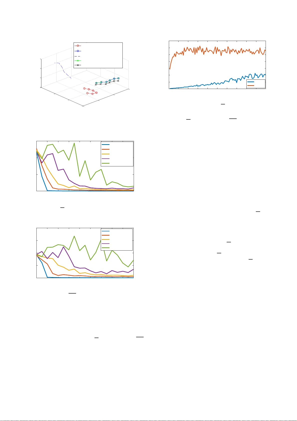
Co op erativ e Lo calisation of a GPS-Denied UA V in 3-Di mensional Space Using Direction of Arriv al Measuremen ts ⋆ James Russell ∗ Mengbin Y e ∗ Brian D. O. Ande rson ∗ , ∗∗ , ∗∗∗ Hatem Hmam ∗∗∗∗ P eter Sarunic ∗∗∗∗ ∗ R ese ar ch Scho ol of Engine ering, Austr alian National University, Canb err a, A.C.T. 2601, Austr alia ∗∗ Hangzhou Dianzi University, Hangzhou, Zhejiang, China ∗∗∗ Data61-CSIR O (formerly NICT A Ltd.) ∗∗∗∗ Austr alian Defenc e Scienc e and T e chnolo gy Gr oup (DST Gr oup) E-mail: { u5542624, men gbin.ye, brian.anderson } @anu.e du.au { hatem.hmam, p eter.sarunic } @dsto.defenc e.gov.au Abstract: This pap er presents a nov el appr oac h for lo calising a GPS (Global Positioning System)-denied Unmanned Aerial V ehicle (UA V) with the aid of a GPS-eq uipped UA V in three-dimensional space. The GPS-equipp ed UA V ma k es discre te- time broadcasts of its global co ordinates. The GPS-denied UA V simultaneously receives the broa dcast and takes direction o f arriv al (DOA) measurements tow ar ds the orig in of the broadcast in its lo cal co ordinate fra me (obtained via a n inertial navigation system (INS)). The aim is to determine the difference betw een the lo cal and global fra mes, descr ibed by a rota tion and a translatio n. In the noiseless case, global co ordinates were recovered exa ctly b y so lving a system of linear equa tio ns. When DOA measurements ar e contaminated with noise, rank relaxed s e midefinite pro gramming (SDP) and the Or thogonal Pro crustes algorithm are employ ed. Sim ula tions ar e provided and factors affecting a ccuracy , such a s noise lev els a nd num ber of measurements, a re explored. Keywor ds: Lo calisation, Direction o f Arriv al Mea suremen t, GPS Denial, Semidefinite Progr amming, Ortho gonal Pr ocrus tes Algorithm, Two-agent netw ork 1. INTRODU CTION Unmanned aer ial v e hic le s play a c en tral role in many de- fence r econnaissance a nd surveillance ope rations. F orma- tions o f UA Vs ca n provide greater reliability and cov er age when compared to a single UA V. T o provide meaningful data in such op erations, all UA Vs in a forma tion must use a single reference frame (t ypically the g lobal fra me). T r a - ditionally , UA Vs have acce s s to the glo ba l fra me via GPS. How ever, GPS sig nals may b e lost in urban en vir onmen ts and enem y controlled airs pace (jamming). Without acces s to glo bal co ordinates, a UA V must r ely on its inertia l navigation system (INS). Positions in the INS frame are upda ted b y in teg rating mea suremen ts from gy- roscop es and accelerometer s. Error in these measur emen ts causes the INS frame to accumulate drift. At any given time, drift is characterised by rotation a nd trans lation with r espect to the glo bal fra me, and is assumed to b e independent b et ween UA Vs in a formation. The error in gyrosc ope a nd accelero meter rea dings is sto c has tic. As a result, INS fra me drift ca nnot be mo delled deterministi- cally . Infor mation from b oth the globa l and INS frames m ust b e collected and used to determine the drift b et w een ⋆ This work was supp orted by the Australian Research Council (AR C) under the ARC grants DP-130103610 and DP-160104500, and b y Data61-CSIR O (formerly NICT A). frames. This pro cess is describ ed as co op e rativ e lo calisa - tion when multiple vehicles provide informatio n. V arious measurement t yp es such as distance betw een agents and directio n of ar riv al of a signal (we henceforth call DOA) can b e used for this pr ocess. In the context of unmanned flight, a dditional s e nsors a dd weight and consume p o w er. As a r e sult, one generally aims to minimise the num b er of measurement t yp es r equired for lo calisation. This pap er s tudies a coo perative approach to lo calisation using DOA mea suremen ts . W e b egin a review of e xisting litera ture by distinguishing lo calisation from tracking. A tracking problem typically inv olves up dating a so lution in re al time, as new mea- surements a re made av a ilable. T racking is p erformed using Bay esia n filter s s uch a s particle filters (Lin and W ei, 2 013) and the Extended Kalman Filter (Chang and F ang, 20 1 4). In lo calisation, a s et of measure ments co llected over a time interv al is used to compute a so lution a t the end of the interv al. A dynamic mo del is t y pically no t requir ed in lo calisation, and is not used in this paper . In (T ekdas and Isler, 201 0), a targ et is lo calised using bea ring 1 mea- surements taken in the glo bal frame by a statio nary sensor net work. In (Duan et al., 20 12), self-lo calisation o f a ro b ot 1 The term b earing i s used int erc hangeably with direction of arri v al (DO A) in a tw o-dimensional ambien t space. How ever, w e ref rain from using i t in three-dimensional am bien t space is achiev ed by taking b earing -only measurements from the rob ot’s INS frame tow ards a set of known global p osi- tions. (Bayram et al., 20 16) demonstrates how an agent is a ble to lo calise a sta tio nary target using b earing -only measurements. Optimal path planning algo rithms a llo wing GPS-enabled sensing ag en ts to lo calise a fixed target are studied in (Lim and Bang , 2014 ). (Y e et a l., 2017) prop osed a method of self-lo calisation o f t wo agents using bea ring measurements but ea c h ag en t was r estricted to statio na ry t wo-dimensional circular orbit. Sim ulta neous lo calisation and mapping (SLAM) metho ds allow for self-lo calisation using o nly INS positio ns and bea ring measurements (Bai- ley , 2 003). The lo cal frame is anchored by p ositions of landmarks which ar e g e nerally sta tionary in the global frame a nd known a priori or contin uously s ensed. The pro blem addressed in this pap er is to lo calise a GP S- denied UA V, whic h we will ca ll Agent B, with the ass is- tance of a nea rb y GPS-enabled UA V, which we will call Agent A. Agent A br oadcasts its globa l coo rdinates at dis- crete instants in time. Both agents move ab out a rbitrarily in three-dimensiona l space. Using each broadc a st of Agent A, Agent B is a ble to take a DOA measure ment tow a rds Agent A. This problem and the solution prop osed in this paper a re nov el. In par ticular, while the literature discussed ab ov e considers certain asp ects from the following list, none consider all of the following as p ects s imultaneously: • The net work co ns ists of only tw o mobile age nts (and is therefo r e different to the senso r netw or k lo calisation problems in the literature). • There is no a pr iori knowledge or sensing of a s tation- ary reference p oint in the global frame. • The UA Vs execute unconstrained arbitrar y motion in three-dimensional space. • Co oper a tion b et ween a GPS-enabled and a GPS- denied UA V (transmissio n o f signals is unidirec tio nal; from Agent A to Agent B. (Zhang et a l., 2 0 16) studied this problem in tw o-dimensio na l space using b earing mea suremen ts . One single piece of data is acquired at each time step. As is detailed in the sequel, tw o sc a lar quantities are obtained with each DOA measurement in the three- dimensional case. The r est of the pap er is struc tur ed as follows. In Section 2 the pro blem is formalised. In Section 3 a solution to the noiseless case is pr e sen ted. Section 4 extends this metho d to allow for noise in DOA measurements. Section 5 presents s im ulation results for the noisy ca se, s tudying the s a me ex ample tr a jectory and a set of Mo n te Carlo simulations. The paper is concluded in Section 6. 2. PROBLEM DEFINITION Two a gen ts, whic h w e call Agent A and Agent B, follow arbitrar y tra jectories in three-dimens ional space. Agent A is able to self-lo calise in the global fra me and therefo r e navigates with r espect to the glo bal frame. Because Agent B is GPS-denied, it has no self-lo calisation c apacit y in the global frame, but ca n self-lo calise in a n INS frame. This INS fra me drifts with r espect to the glo ba l fra me ov er long per iods, but can b e considered constant in short interv als. Positions each of ag en t in their navigation frames and DOA measurements of signals betw e en agents ar e ob- tained through a discrete-time measurement pro cess. W e let P I J ( k ) denote the p osition of a g en t J in the co o rdinate frame of age nt I at a k th time instant. Time b et ween measurements can b e v ariable. Let u , v , w deno te g lobal frame co ordinates, and x , y , z denote coo rdinates in the INS frame of Agen t B. Position co ordinates at time instant k are expressed as follows: P A A ( k ) = [ u A ( k ) v A ( k ) w A ( k )] ⊤ (1) P B B ( k ) = [ x B ( k ) y B ( k ) z B ( k )] ⊤ (2) Agent B’s INS frame evolv es via drift which, at a partic- ular time instant, c a n b e mo delled as a ro tation and a translation from the global frame. The rota tion and or igin of the INS fra me is considered to b e time inv ar ia n t over short interv als, during which the following measure men t pro cess can o ccur m ultiple times. At each time instant k : • Agent A r ecords and broa dcasts its p osition in the global frame, i.e. P A A ( k ). • Agent B recor ds its o wn pos ition in the INS frame, i.e. P B B ( k ). • Agent B r eceiv es the broadca st from Agent A, and measures the signal’s DOA in the INS frame of B . Receipt of a broa dcast may trigger the use of a n optical s ensor W e assume the delay b et ween Agent A se nding its co ordi- nates and Ag en t B receiving this infor mation is negligible, i.e. w e assume the three activities occur simultaneously . The a im is to ex pr ess the co ordinates of Agent B in the global fra me, in o ther words to determine: P A B ( k ) = [ u B ( k ) v B ( k ) w B ( k )] ⊤ (3) Passing betw e en the global frame and the INS frame of Agent B is a c hieved by a rotation of frame axes and translation of origin p oin t of the frame. F or instance, the co ordinates v ector of Age nt A in the INS frame of Ag e nt B is obtained as follows: P B A = R B A P A A + T B A (4) Therefore we hav e P A B = R B ⊤ A ( P B B − T B A ) whe r e R B ⊤ A = R A B and − R B ⊤ A T B A = T A B . The lo calisation problem ca n therefore b e reduced to solving for the entries o f R B A ∈ S O (3) indexed r ij and T B A ∈ R 3 indexed t i . Direction of arriv al mea suremen ts taken by Agent B towards Agent A ar e per formed by instruments fix e d to the bo dy o f Agent B. It is assumed that through the use of attitude measurements in the INS frame, Agent B is a ble to conv ert DOA r eadings from its b o dy fixed frame to a b o dy centred frame with the same orientation (rotation) as its INS frame. Direction of arriv al in Agent B ’s b ody centred fra me with the same orientation a s its INS fra me is therefore expressed using the following spheric a l co ordinate system: • Azimu th ( θ ): angle formed betw een the p ositive x ax is and the pro jection the vector from Agent B tow ar ds Agent A onto xy plane. • Elev ation ( φ ): a ngle formed betw een unit vector to- wards Agent A and xy plane. The angle is positive if the z c omponent of the unit vector tow ards Agen t A is pos itiv e. The total num b er of scalar measurements r equired to solve the lo calisation problem cannot b e sma lle r than the nu mber of degrees o f freedom in the rotation matrix a nd translation vector. Note that R B A is a rotatio n matrix ( R B A ∈ S O (3)), with p ossible par ametrisations including Euler angles and Rodr igues pa r ametrisation. W e work directly with entries r ij to o btain linear problems. E uler angle pa rametrisation of R B A is a 3 vector. The translation vector is a 3 vector. This pro blem therefore has 6 deg rees of freedom. The matrix R B A is a rotation matrix if and only if R B A R B ⊤ A = I 3 and det( R B A ) = 1. As will b e seen in the sequel, these constraints are equiv alent to a set of quadratic constra in ts on e ntries of R B A . In total ther e a re 12 entries of R B A and T B A to b e found. An equation set of n indepe ndent rela tions (including measur emen ts and constraints) for n v ar iables will ge nerically hav e multiple solutions if at least one of the r e la tions is quadr atic. When an additional scalar mea s uremen t is taken, g e nerically a unique solution exis ts . 3. LOCALISA TION WITH NOISE L ESS MEASUREMENTS This section co ns iders noiseless p osition and dir ection of ar r iv a l measuremen ts. Section 4 consider s noise in direction of ar riv al measurements only . The consideration of noisy p osition mea suremen ts is left for future work. 3.1 F orming a system of line ar e quations A unit vector in the INS frame, p oin ting fr o m Agent B to Agent A, de fined by azimuth and e le v a tion a ngles θ a nd φ , ca n b e par ametrised as fo llows: ˆ d ( θ , φ ) = [ cos θ co s φ, sin θ cos φ, sin φ ] ⊤ (5) The following static analy sis ho lds for all instants in time, hence the specificatio n k is dropped. Define ¯ d . = k P A B − P B B k as the E uclidean distance b et ween Agent A and Agent B (whic h is not a v ailable to either ag en t). Scaling the unit vector ¯ d g iv es ˆ d ( θ, φ ) = 1 ¯ d [ x A − x B , y A − y B , z A − z B ] ⊤ (6) Applying equation (4) yields: " cos θ co s φ sin θ cos φ sin φ # = 1 ¯ d " r 11 u A + r 12 v A + r 13 w A + t 1 − x B r 21 u A + r 22 v A + r 23 w A + t 2 − y B r 31 u A + r 32 v A + r 33 w A + t 3 − z B # (7) The left hand v ector is calculated direc tly fr o m DOA measurements. Each entry o f the vector on the right hand side is a linear combination of e ntries of R B A and T B A . Cross- m ultiplying entries 1 and 3 o f b oth vectors eliminates ¯ d , a nd yields the following equality: sin φ ( r 11 u A + r 12 v A + r 13 w A + t 1 − x B ) = cos θ co s φ ( r 31 u A + r 32 v A + r 33 w A + t 3 − z B ) (8) which for con venience is rear ranged as ( u A sin φ ) r 11 + ( v A sin φ ) r 12 + ( w A sin φ ) r 13 − ( u A cos θ co s φ ) r 31 − ( v A cos θ co s φ ) r 32 − ( w A cos θ cos φ ) r 33 + (sin φ ) t 1 − (cos θ cos φ ) t 3 = (sin φ ) x B − (cos θ cos φ ) z B (9) Similarly , cro ss-m ultiplying en tries 2 a nd 3 of b oth vectors app earing in equation (7) yields a similar equation. ( u A sin φ ) r 21 + ( v A sin φ ) r 22 + ( w A sin φ ) r 23 − ( u A sin θ cos φ ) r 31 − ( v A sin θ cos φ ) r 32 − ( w A sin θ cos φ ) r 33 + (sin φ ) t 2 − (sin θ cos φ ) t 3 = (sin φ ) y B − (sin θ cos φ ) z B (10) Both equations (9) a nd (10) are linear in the unknown r ij and t i terms. Given a series of K measurements, these equations c an b e use d to construct the following system of linear equations: A Ψ = b (11) where the 12- v ector o f unknowns Ψ is defined a s: Ψ = [ r 11 r 12 r 13 ... r 31 r 32 r 33 t 1 t 2 t 3 ] ⊤ (12) The matrix A con tains the known v alues P A A ( k ) and φ ( k ) , θ ( k ) for k = 1 , ..., K . The v e ctor b contains the known v alues P B B ( k ) a nd φ ( k ) , θ ( k ) for k = 1 , ..., K . The precise forms of A and b are omitted due to spatial limitations, and will b e included in an extended version of the pa per. 3.2 Example with noiseless DOA me asur emen ts If K ≥ 6, the ma trix A will b e square or tall. In the noise- less case, if A is of full column ra nk, equatio n (11) will be solv able. W e demonstrate this using a set of example tra- jectories detailed in T able 1. W e w ill make additional use of this example tra jectory in the noisy measurement case presented in Section 5. Extens ive Monte Car lo sim ulatio ns demonstrating lo calisation for a larg e num b er of g eneric flight tra jector ie s are left to the nois y measurement case. Nongeneric flight tra jectories are discussed immediately below, in subsection 3.3. Example tra jectories for Agents A and B in the glo ba l frame were g enerated. These tra jectories sa tisfied a set of flight pr o perties to b e included in the extended v ersion of this pap er. These ar e plotted in Figure 1. The r otation matrix and transla tio n vector used in sim ula tion are: R B A = " − 0 . 627 − 0 . 776 0 . 072 − 0 . 747 0 . 6 25 0 . 228 − 0 . 222 0 . 0 90 − 0 . 971 # (13) T B A = [ 247 . 49 0 110 . 38 2 229 . 78 4 ] ⊤ (14) T able 1 includes azimuth a nd elev atio n ang le mea s ure- men ts fr om Agent B tow ards Agent A in the measurement frame, for K = 6 time instants. Using (11), R B A and T B A were so lv ed exactly for the given flig h t tra jectorie s . 3.3 Nongeneric tr aje ctories It is ob vious that w e can o nly lo calise Agent B by so lving (11) if matrix A ha s full co lumn rank. W e are therefor e motiv ated to iden tify tra jectories of Agen t A and Agent B which result in ra nk ( A ) < 6 (assuming K ≥ 6) so we can av oid them. A la r ge n umber of simulations revealed that r ank( A ) < 6 is cons isten tly encountered for all K ≥ 6 when the tra jectory of Agent A is restricted to a plane. Note that this plane need not b e pa rallel to a co ordinate plane of either the global or INS co ordina te fra mes. W e leav e further, detailed analytical treatment of nongener ic tra jecto ries to the extended version o f this pa p er. T able 1. Positions of Agents A and B in their resp ectiv e frames and nois e less DOA meas ur e- men ts for exa mple tr a jectories Time k P A A DOA [ θ φ ] P B B 1 [0 0 300] ⊤ [-1.500 -0.851] [89 . 680 1035 . 199 474 . 865] ⊤ 2 [82 . 962 − 235 . 407 314 . 161] ⊤ [-1.679 -0.835] [ − 40 . 633 1157 . 514 649 . 672] ⊤ 3 [141 . 084 − 478 . 270 302 . 352] ⊤ [-1.789 -0.812] [ − 182 . 218 1255 . 810 830 . 757] ⊤ 4 [139 . 079 − 726 . 308 271 . 157] ⊤ [-1.977 -0.733] [ − 165 . 197 1416 . 859 1021 . 213] ⊤ 5 [ − 109 . 876 − 704 . 457 277 . 792] ⊤ [-1.828 -0.790] [ − 217 . 778 1581 . 963 1201 . 424] ⊤ 6 [ − 252 . 217 − 499 . 403 291 . 634] ⊤ [-1.499 -0.833] [ − 452 . 605 1649 . 158 1254 . 728] ⊤ 4. LOCALISA TION WITH NOISY DOA MEASUREMENTS In practice, DOA measurements from s ensors on Ag en t B will b e co n taminated with noise. This section develops an approach to dea l with the no isy measurements which are encountered in real-world implement ation. W e approa c h the pr oblem using semidefinite programming to exploit the quadratic constraints on Ψ arising from the pro perties of the rotation matrix. Such constra in ts would not b e utilised in a standar d unco nstrained least squares a pproach. In practice, no ise contaminated azimuth and elev ation measurements a re ta ken in the bo dy fixe d frame of Agen t B. Strictly sp eaking, the noise is exp ected to follow a v on Mises distribution (F o rbes et al., 2 0 11). F o r sma ll noise, such as wha t we enco unter, the von Mises distribution can b e approximated by a Gaussian distribution. The noise affecting az im uth and e le v atio n a re a ssumed to b e independent when measured in the b ody fixed frame, how ever they ar e not known to hav e equal sta ndard deviations. These no ises ar e likely to lo se indep endence when azimuth and elev a tion measurements measured in the b ody fixed fra me are conv er ted into azimuth and elev ation v alues in Agent B’s b ody centred frame with the same o rien ta tion as its INS frame. 4.1 Qu ad r atic c onst ra ints on ent ries of Ψ W e now identify 21 qua dratic constraints o n entries of R B A . Note that this set is not indepe nden t, as discusse d in Remar k 1 b elow. Rec a ll the or thogonality pr operty R B A R B ⊤ A = I 3 . By co mputing each entry of R B A R B ⊤ A and setting these equal to en tr ie s o f I 3 , we define constr ain ts C i for i = 1 , ..., 6: C 1 = ψ 2 1 + ψ 2 2 + ψ 2 3 − 1 = 0 (15a) C 2 = ψ 2 4 + ψ 2 5 + ψ 2 6 − 1 = 0 (15b) C 3 = ψ 2 7 + ψ 2 8 + ψ 2 9 − 1 = 0 (15c) C 4 = ψ 1 ψ 4 + ψ 2 ψ 5 + ψ 3 ψ 6 = 0 (15d) C 5 = ψ 1 ψ 7 + ψ 2 ψ 8 + ψ 3 ψ 9 = 0 (15e) C 6 = ψ 4 ψ 7 + ψ 5 ψ 8 + ψ 6 ψ 9 = 0 (15f ) T o simplify notation we call C j : k the set o f constra in ts C i for i = j, .., k . Similarly , by co mputing each entry of R B ⊤ A R B A and setting these equa l to I 3 , w e define constraints C 7:12 . W e omit presentation of C 7:12 due to spatial limitations and similarity with C 1:6 . The sets C 1:6 and C 7:12 are clearly equiv alen t. F urther constraints a re required to ensure det( R B A ) = 1. Cramer’s fo rm ula states that R B A − 1 = adj( R B A ) / det( R B A ), where adj( R B A ) denotes the adjugate matrix of R B A . Or- thogonality of R B A implies R B A ⊤ = adj( R B A ) or that R B A = adj( R B A ) ⊤ . By computing en tries o f the first column of Z = R B A − a dj( R B A ) ⊤ and setting these equal to 0, we define constraints C 13:15 : C 13 = ψ 1 − ( ψ 5 ψ 9 − ψ 6 ψ 8 ) = 0 (16a) C 14 = ψ 4 − ( ψ 3 ψ 8 − ψ 2 ψ 9 ) = 0 (16b) C 15 = ψ 7 − ( ψ 2 ψ 6 − ψ 3 ψ 5 ) = 0 (16c) Similarly , by co mputing the en tr ies of the seco nd and third columns of Z a nd setting these equal to 0 , we define constraints C 16:18 and C 19:21 . Due to space limitations, we omit pr esen ting them. The complete set C 1:21 constrains R B A to be a rotation ma trix. W e refer to this set as C Ψ . Due to these a dditional relations, lo calisation requir e s azimuth and elev a tio n measurements at 4 insta nts only ( K = 4 ), as oppo sed to 6 instants requir ed in Section 3. 4.2 F ormulation of the S emid efinite Pr o gr am The go al of the semidefinite progra m is to o btain: argmin Ψ || A Ψ − b || (17) sub ject to C Ψ . Equiv alently , we seek a rgmin Ψ || A Ψ − b || 2 sub ject to to C Ψ . W e define the inner pro duct o f t wo matrices U and V as h U, V i = trace( U, V ⊤ ). O ne obtains || A Ψ − b || 2 = h P, X i (18) where P = [ A b ] ⊤ [ A b ] and X =  Ψ − 1   Ψ − 1  ⊤ (19) and X is a rank 1 p ositive-semidefinite ma trix 2 . The constraints C Ψ can also b e ex pr essed in inner pro duct form. F or i = 1 , ..., 21, C i = 0 is equiv alen t to h Q i , X i = 0 for s ome Q i . Solving for Ψ in (17 ) is therefor e equiv alent to so lving for: argmin Ψ h P, X i (20) such that: X ≥ 0 (21) rank( X ) = 1 (22) X 13 , 13 = 1 (23) h Q i , X i = 0 (24) for i = 1 , ..., 2 1. This fully defines the semidefinite pro- gram. R emark 1. (Inclusion of Dep enden t Co ns train ts). Note that while the set of equations (15) and (16) for m an independent set of co nstrain ts on the first nine ent ries of Ψ, the set of cons tr ain ts C Ψ is not indep endent . F or instance, C 1:6 and C 7:12 are equiv a len t. F or simplicity , we use C Ψ in the SDP formulation in this paper . In the extended version of this pap er, we will thor oughly 2 All matrices M whic h can b e expressed in the f orm of M = v v ′ where v is a column vec tor are p ositiv e-semidefinite matrices. inv estigate whether lo calisation accuracy improv es with the a dditional dep enden t constraints. R emark 2. (Normalisation of tra nslation terms). It was ob- served that SDP so lutio n a c curacy deteriora tes when the condition num ber of X of the true s o lution is high. When approximate size of T B A is known, co efficients asso ciated to ent ries t i in equations (9) and (10) are scaled to solve for v a lues close to 1 . 4.3 Ra nk R elaxation of Semidefinite Pr o gr am This semidefinite progr am is a r eform ula tion of a qua drat- ically constrained quadra tic pro gram (QCQP). Computa- tionally sp eaking, QCQ P problems are genera lly NP-hard. A close a ppro x ima tion to the tr ue solution can be o bta ined in po ly nomial time if the rank 1 constra in t o n X is r e laxed. The s o lution to the relaxe d semidefinite prog ram X is t ypically clo se to b eing a ra nk 1 matrix 3 . The closest rank 1 approximation to X , which we ca ll ˆ X , is obtained by ev aluating the sing ular v alue decomp osition of X , then setting a ll singular v alues except the larg est eq ua l to z ero. F rom ˆ X , one ca n then use the definition of X in (19) to obtain the approximation of Ψ , which we will call ˆ Ψ. Entries ˆ ψ i for i = 10 , 11 , 12 can b e us e d immediately to construct an estima te fo r T B A , which we will call T . Entries ˆ ψ i for i = 1 , ..., 9 will b e used to c onstruct an approximation of R B A , whic h we will call b R . 4.4 Ort ho gonal Pr o crustes Pr oblem Due to the relaxation of the rank constraint on X , it is no longer g uaran teed that en tries of ˆ Ψ strictly satisfy the set of co nstrain ts C Ψ . Sp ecifically , the ma trix b R may not be a rotation matrix. The Orthogonal Pro crustes a lgorithm is a c o mmonly used to ol to determine the closest o r thogonal matrix (denoted R ) to a given matrix, b R . This is given by R = argmin Ω || Ω − b R || F sub ject to ΩΩ ⊤ = I , where || . || F is the F robenius norm. When noise is high, the ab ov e method o ccasiona lly returns R such that det( R ) = − 1. A sp ecial ca s e of the Orthogonal Pro crustes alg o rithm is av a ilable to ensure tha t det( R ) = 1, i.e. R ∈ S O (3) is a pro p er ro ta tion matrix but w e omit the mino r details due to spatial limitations. The matrix R and vector T are the final approximations of R B A and T B A using the combination of the semidefinite pro- gram and Orthogona l P r ocrus tes metho ds. The estimate of the p osition of B in the glo bal frame is P A B = R ⊤ ( P B B − T ). 4.5 Metrics for err or in R and T This pap er uses the geo desic metric for rota tio n. This metric on S O (3) defined by d ( R 1 , R 2 ) = ar ccos  tr( R ⊤ 1 R 2 ) − 1 2  (25) is the magnitude of a ngle of ro tation ab out this axis (T ron et al., 2016 ). Where R B A is known, the err or of 3 The measure used for closeness to rank 1 is the ratio of the tw o largest singular v alues in the singular v alue decomp osition of X . T able 2. Positions of P A B and P A B , and Gaussian noise ( σ = 3 ◦ ) added to a zim uth and elev a tion measurements ( ζ 1 , ζ 2 ∼ N (0 , σ 2 )) Time k P A B [ ζ 1 ζ 2 ] [rads] P A B [ ζ 1 ζ 2 ] [degs] 1 [800 0 350] ⊤ [0.0747 -0.0637] [695 . 7 − 61 . 6 309 . 1] ⊤ [4.2809 -3.6483] 2 [1017 . 5 − 122 . 5 364 . 1] ⊤ [-0.0350 0.0699] [902 . 6 − 201 . 4 321 . 9] ⊤ [-2.0029 4.0065] 3 [1225 . 7 − 260 . 8 358 . 0] ⊤ [-0.0478 -0.1032] [1098 . 9 − 355 . 9 314 . 3] ⊤ [-2.7416 -5.9145] 4 [1474 . 1 − 233 . 5 363 . 9] ⊤ [0.0243 0.0084] [1348 . 7 − 348 . 8 320 . 9] ⊤ [1.3943 0.4801] 5 [1719 . 3 − 272 . 8 392 . 6] ⊤ [-0.0247 0.0165] [1589 . 9 − 408 . 2 349 . 5] ⊤ [-1.4124 0.9474] 6 [1810 . 6 − 496 . 1 458 . 0] ⊤ [0.0937 -0.0031] [1662 . 8 − 639 . 0 412 . 0] ⊤ [5.3698 -0.1750] rotation R is defined as d ( R , R B A ). Position error is defined as the average Euclidia n distance b e t ween true glo bal co ordinates o f B, and estimated global co ordinates ov er the K measur emen ts taken. err or ( P A B ) = P k || R B ⊤ A ( P B B ( k ) − T B A ) − P A B ( k ) || K (26) 5. SIMULA TION RESUL TS In this s e c tion, we inv estigate the p erformance of the SDP algor ithm combined with the Orthog onal Pro crustes Algorithm in the presence of noise (w e shall ca ll this combined alg o rithm SDP+ O for sho rt). W e acknowledged in Section 4 that noise in measurements of θ ( k ) a nd φ ( k ) may not hav e the same standa rd deviations. Howev er, fo r simplicity a nd with space limitations in mind, we will assume in this pap er that the standard dev ia tions a re the same (which we denote a s σ ). In o ther words, e θ ( k ) = θ ( k ) + ζ 1 and e φ ( k ) = φ ( k ) + ζ 2 where ζ 1 , ζ 2 ∼ N (0 , σ 2 ) Extensive exploratio n of different standard deviations for θ ( k ) and φ ( k ) will be conducted in this pa per’s extended version. 5.1 Example with noisy DOA me asur ements Samples of Gaussian err or with µ = 0 ◦ , σ = 3 ◦ were added to ele v atio n and azimu th measurements s im ulated in Section 3.2. The SDP+O algor ithm was used to obtain of R and T . The reconstr ucted tra jectory P A B is plotted in Figure 1 . Position data o f the r econstructed tra jectory P A B and simulated noise contaminating azimuth and elev a tio n readings is tabulated in T able 2 . 5.2 Monte Carlo Simulations on R andom T r aje ctories In this subsection, we conduct extensive Monte Carlo s im- ulations to sho w the viabilit y of the SDP+O algo rithm. W e randomly genera ted 10 0 r e alistic fixe d wing UA V tr aje cto- ries . By rea listic, we mean that the distance separatio n betw een successive measurements is consistent with UA V flight sp eeds a nd ensures the UA V do es not ex ceed an upper b ound on the turn/ clim b r a te. W e v ary the noise level by σ = 0 . 1 ◦ , 1 ◦ , 2 ◦ , 3 ◦ , 5 ◦ . The nois e level σ = 0 . 1 ◦ is 0 2000 500 2000 1000 w coordinate 1500 1000 1000 v coordinate u coordinate 0 0 -1000 -1000 P A A (global coordinates of A) P B A (global coordinates of B) P B B (coordinates of B in frame of B) Noiseless solution using (14) SDP+O Estimate of P B A (noisy) Fig. 1. Recovery o f globa l co ordinates o f Agent B for example tr a jectories (er ror of σ = 3 ◦ in noisy cas e) 2 4 6 8 10 12 14 16 18 20 Number of DoA measurements 0 50 100 150 Median rotation error in degrees σ = 0.1 degrees σ = 1 degree σ = 2 degrees σ = 3 degrees σ = 5 degrees Fig. 2. Media n d ( R , R B A ) vs. nu mber of DOA mea s ure- men ts used to solve SDP + O. 2 4 6 8 10 12 14 16 18 20 Number of DoA measurements 0 500 1000 1500 2000 Median position error in metres σ = 0.1 degrees σ = 1 degree σ = 2 degrees σ = 3 degrees σ = 5 degrees Fig. 3. Me dia n er ror ( P A B ) vs. num b er of DOA measure- men ts used to solve SDP+O (av er age dis tance of 1.38km b et ween agents). representative of an optical senso r, while o ther noise levels are repres en tative of antenna-based (RF) measurements. F or each level o f nois e , we conducted 100 Monte Ca rlo simulations with unique tra jectories . F or each noise level, we then calculated the median d ( R, R B A ) and er ror ( P A B ) ov er the 10 0 simulations. Median is a commonly used a s measure of central tendency to mitigate the effect o f outlier s. W e use this measure to analyse Monte Ca rlo simulation results. Discussion on the cum ulative frequency distribution of er rors obtained for each set of 100 Mont e Carlo simulations will b e included in the extended version of this pap er. 0 0.5 1 1.5 2 2.5 3 3.5 4 4.5 5 DoA measurement error σ (azimuth and elevation) 0 20 40 60 80 100 120 140 Median rotation error of R in degrees SDP+O LS+O Fig. 4. Compar is on of median d ( R, R B A ) us ing SDP+O and LS+O methods for example tra jectory ( K = 6). The media n d ( R, R B A ) and er ror ( P A B ) versus the num- ber o f measurements (i.e. K ) used to solve the SDP+O are plotted in Figure 2 a nd Fig ure 3, r espectively . It is observed that for ea c h v a lue of σ there is g reater im- prov ement in r otation error than translation e r ror as K is inc r eased. This will be discus s ed further in the extended version of this pap er. 5.3 Comp arison of LS+O and SDP+O In this subsection, we co mpa re the SDP+O algorithm with a n unconstrained Lea st Squares a lg orithm co m bined with the O rthogonal P rocr ustes alg orithm (whic h we ca ll LS+O). By LS+O , we mean that Ψ ∗ = ar gmin Ψ k A Ψ − b k is found witho ut any c o nstrain ts on Ψ. The first nine ent ries of Ψ a r e then used to form a matrix, a nd the O r - thogonal Pro crustes algorithm detailed in subsection 4.4 is applied to obtain the clos est ro tation matrix R . Agents A and B a re prescrib ed the representativ e tra jec- tories illustrated in Figur e 1. Noise level was v aried from σ = 0 ◦ to 5 ◦ . F or ea ch noise le v el, we conducted 20 Monte Carlo simulations of the same tra jectory using LS+O and SDP+O . The er ror index d ( R, R B A ) was se pa rately calculated ov er the 20 s im ulations for LS+ O a nd SDP+O. Figure 4 shows the median d ( R, R B A ) versus level of noise for bo th LS+O and SDP+ O. The median d ( R, R B A ) using the LS+O algor ithm was consis ten tly double that using the SDP+O metho d. Median error s in the order of 90 ◦ are exp ected from a r andom set of rotation matr ices. W e conclude that SDP+O is the supe rior metho d. Its median per formance is approximately linear in the mean azimuth and elev a tio n mea suremen t erro r s ta ndard dev iation. 6. CONCLUSION This pap er studied a co op erative lo calisation problem b e- t ween a GPS- denied and a GP S-enabled UA V. The GPS- enabled UA V broadcas ts it po sition in discr ete time to the GPS-denied UA V, and the GP S-denied UA V measures the direction of arriv a l of the broadcast signal. It w as found that lo calisation could b e achiev ed by so lving a non-linea r system with less than 6 DOA meas uremen ts. A lo calisation algorithm was developed in tw o sta ges. With noiseless DOA meas uremen ts, we show ed that a linear sys tem o f equations built from six or mo re measur emen ts yielded the lo calisation s olution for gener ic tra jectories. The sec o nd stage considered noisy DOA measur emen ts. An optimisa- tion pro blem w as defined in which the ob jective function and co nstrain ts on its ar gumen ts were qua dratic. This problem therefore lent itse lf to quadratically c o nstrained quadratic pr ogramming, which was solved numerically us- ing a rank relax e d semidefinite progr a m with the solution adjusted using the Ortho g onal Pro crustes algorithm. Sim- ulations were pr esen ted to illus trate the algorithm when DOA measurements were noisy . F uture work includes im- proving the r eliabilit y of the SDP+ O metho d, studying m ultiple a gen ts in a formatio n a nd filtering metho ds. REFERENCES Bailey , T. (2003). Constrained initialisa tion for bea ring- only slam. In R ob otics and Automation, 2003. Pr o- c e e dings. ICRA ’03. IEEE International Confer enc e on , volume 2, 19 66–1971 vol.2. Bayram, H., Ho ok, J.V., and Isler, V. (201 6 ). Gathering bea ring data for targ et lo calization. IEEE Ro b otics and Automation L etters , 1(1), 369 –374. Chang, D.C. a nd F a ng , M.W. (2014). Bearing- o nly ma- neuvering mobile tra c king with nonlinear filtering a l- gorithms in wireless sensor netw o rks. IEEE Systems Journal , 8(1), 16 0–170. Duan, Y., Ding, R., and Liu, H. (2012). A pro babilistic metho d of b earing-only lo calizatio n by using omnidi- rectional vision signal pro cessing. In Intel ligent Infor- mation Hiding and Mult ime dia Signal Pr o c ess ing (IIH- MSP), 2012 Eighth Intern atio nal Confer enc e on , 285– 288. F orb es, C., Ev ans, M., Hastings, N., and Peacock, B. (2011). Statistic al Distributions . John Wiley & Sons. Lim, S. and B ang, H. (201 4 ). Guidance laws for target lo calization using vector field a pproach. IEEE T r ansac- tions on A er osp ac e and Ele ctr onic Systems , 50(3 ), 19 91– 2003. Lin, M. and W ei, Y.D. (2013). Information fusion passive lo cation filtering alg orithm. In 2013 25th Chinese Contr ol and De cision Confer enc e (CCDC) , 1874–1 877. T ekdas, O . and Isler , V. (201 0). Senso r placement for triangulation- based lo calizatio n. IEEE T r ansactions on Automation Scienc e and Engine ering , 7(3), 681– 685. T ron, R., Thomas, J., Loianno, G., Daniilidis , K., and Ku- mar, V. (201 6 ). A distributed optimization framework for lo calization and fo rmation control: Applications to vision-base d meas uremen ts. IEEE Contr ol Systems , 36(4), 22–44. Y e, M., Anderson, B.D.O., a nd Y u, C. (2017 ). Bear ing- only measurement self-loca lization, velo cit y consen- sus and formation co n trol. IEEE T r ansactions on A er osp ac e and Ele ctr onic Systems , av a ilable o nline. doi: 10.110 9/T AES.201 7.2651538. Zhang, L., Y e, M., Anderson, B.D.O., Sarunic, P ., and Hmam, H. (2 0 16). Co op erative lo calisation of uavs in a gps-denied e nvironment using b earing measurements. In 2016 IEEE 55th Confer enc e on De cision and Contr ol (CDC) , 4 320–432 6.