Special Orthogonal Group SO(3), Euler Angles, Angle-axis, Rodriguez Vector and Unit-Quaternion: Overview, Mapping and Challenges

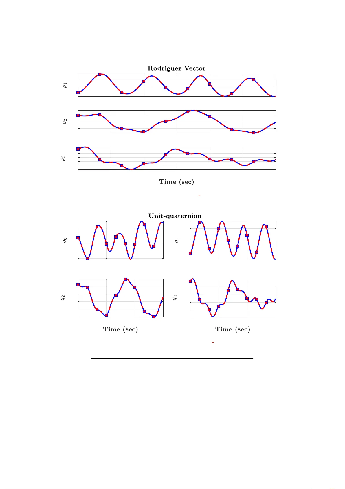
Special Orthogonal Gr oup SO(3), Euler Angles, Angle-axis, Rodriguez V ector and Unit-Quaternion: Overview , Mapping and Challenges Hashim A. Hashim a a Department of Engineering and Applied Science, Thompson Rivers University , BC, Canada, V2C-0C8. Abstract The attitude of a rigid-body in the three dimensional space has a unique and global deﬁnition on the Spe- cial Orthogonal Group SO ( 3 ) . This paper gives an overview of the rotation matrix, attitude dynamics and parameterization. The four most frequently used methods of attitude r epr esentations are discussed with detailed derivations, namely Euler angles, angle-axis parameterization, Rodriguez vector , and unit- quaternion. The mapping from one r epresentation to others including SO ( 3 ) is given. Also, important results which could be useful for the process of ﬁlter and/or control design ar e given. The main weak- nesses of attitude parameterization using Euler angles, angle-axis parameterization, Rodriguez vector , and unit-quaternion are illustrated. Keywords: Special Orthogonal Group 3, Euler angles, Angle-axis, Rodriguez V ector , Unit-quaternion, SO ( 3 ) , Mapping, Parameterization, Attitude, Control, Filter , Observer , Estimator , Rotation, Rotational matrix, T ransformation matrix, Orientation, T ransformation, Roll, Pitch, Y aw . Bibtex formatted citatio n : @article { hashim2019special, title= { Special Orthogonal Group SO(3), Euler Angles, Angle-axis, Rodriguez V ector and Unit-Quaternion: Overview , Mapping and Challenges } , author= { Hashim A. Hashim } , journal= { ArXiv preprint ArXiv:1909.06669 } , year= { 2019 } } T o cite this article: H. A. Hashim, ”Special Orthogonal Group SO(3), Euler Angles, Angle-axis, Rodriguez V ector and Unit-Quaternion: Overview , Mapping and Challenges.” arXiv preprint arXiv:1909.06669, 2019 . Email address: hhashim@tru.ca (Hashim A. Hashim) Contents 1 Introduction 3 2 Preliminaries and Math Notation 5 2.1 SO ( 3 ) Preliminaries . . . . . . . . . . . . . . . . . . . . . . . . . . . . . . . . . . . . . . . . . . 6 2.2 Angle-axis parameterization preliminaries . . . . . . . . . . . . . . . . . . . . . . . . . . . . . 7 2.3 Rodriguez vector preliminaries . . . . . . . . . . . . . . . . . . . . . . . . . . . . . . . . . . . . 7 2.4 Unit-quaternion preliminaries . . . . . . . . . . . . . . . . . . . . . . . . . . . . . . . . . . . . . 8 2.5 Useful math identities . . . . . . . . . . . . . . . . . . . . . . . . . . . . . . . . . . . . . . . . . 8 3 Special Orthogonal Group SO ( 3 ) 8 3.1 Attitude dynamics . . . . . . . . . . . . . . . . . . . . . . . . . . . . . . . . . . . . . . . . . . . 9 3.2 Normalized Euclidean distance . . . . . . . . . . . . . . . . . . . . . . . . . . . . . . . . . . . . 10 3.3 Normalized Euclidean distance dynamics . . . . . . . . . . . . . . . . . . . . . . . . . . . . . . 11 3.3.1 Discrete Attitude dynamics . . . . . . . . . . . . . . . . . . . . . . . . . . . . . . . . . . 11 3.4 Attitude error and attitude err or dynamics . . . . . . . . . . . . . . . . . . . . . . . . . . . . . 13 4 Euler Parameterization 13 4.1 Attitude parameterization through Euler angles . . . . . . . . . . . . . . . . . . . . . . . . . . 14 4.2 Euler angles from SO ( 3 ) . . . . . . . . . . . . . . . . . . . . . . . . . . . . . . . . . . . . . . . . 15 4.3 Angular velocities transformation . . . . . . . . . . . . . . . . . . . . . . . . . . . . . . . . . . 16 4.4 Detailed derivation of Euler rate . . . . . . . . . . . . . . . . . . . . . . . . . . . . . . . . . . . 17 4.5 Euler parameterization problem . . . . . . . . . . . . . . . . . . . . . . . . . . . . . . . . . . . 19 5 Angle-axis Parameterization 19 5.1 Mapping: Fr om/T o unit vector and angle of r otation to/fr om other repr esentations . . . . . . 19 5.2 Problems of angle-axis parameterization: . . . . . . . . . . . . . . . . . . . . . . . . . . . . . . 22 6 Rodriguez V ector Parameterization 22 6.1 Mapping: Fr om/T o Rodriguez vector to/fr om other r epresentations . . . . . . . . . . . . . . 22 6.2 Attitude measurements . . . . . . . . . . . . . . . . . . . . . . . . . . . . . . . . . . . . . . . . . 27 6.3 Rodriguez vector dynamics . . . . . . . . . . . . . . . . . . . . . . . . . . . . . . . . . . . . . . 29 6.4 Attitude error and attitude err or dynamics in the sense of Rodriguez vector . . . . . . . . . . 29 6.5 Problems of Rodriguez vector parameterization: . . . . . . . . . . . . . . . . . . . . . . . . . . 30 7 Unit-quaternion 30 7.1 Quaternion multiplication . . . . . . . . . . . . . . . . . . . . . . . . . . . . . . . . . . . . . . . 31 7.2 Mapping: Fr om/T o unit-quaternion to/fr om other r epresentations . . . . . . . . . . . . . . . 32 7.3 Attitude measurements . . . . . . . . . . . . . . . . . . . . . . . . . . . . . . . . . . . . . . . . . 35 7.4 Unit-quaternion attitude dynamics and measurements . . . . . . . . . . . . . . . . . . . . . . 36 7.4.1 Continuous Unit-quaternion Attitude dynamics . . . . . . . . . . . . . . . . . . . . . . 36 7.4.2 Discrete Unit-quaternion Attitude dynamics . . . . . . . . . . . . . . . . . . . . . . . . 36 7.4.3 Sensor Measurements . . . . . . . . . . . . . . . . . . . . . . . . . . . . . . . . . . . . . 37 7.5 Rotational acceleration . . . . . . . . . . . . . . . . . . . . . . . . . . . . . . . . . . . . . . . . . 38 7.6 Unit-quaternion update . . . . . . . . . . . . . . . . . . . . . . . . . . . . . . . . . . . . . . . . 38 7.7 Unit-quaternion error and err or derivative . . . . . . . . . . . . . . . . . . . . . . . . . . . . . 38 7.8 Problem of unit-quaternion . . . . . . . . . . . . . . . . . . . . . . . . . . . . . . . . . . . . . . 40 8 Simulation 41 9 Conclusion 48 2 List of T ables 1 Mathematical Notation . . . . . . . . . . . . . . . . . . . . . . . . . . . . . . . . . . . . . . . . . 5 2 Attitude Notation . . . . . . . . . . . . . . . . . . . . . . . . . . . . . . . . . . . . . . . . . . . . 6 3 Initial conditions - Example 1 . . . . . . . . . . . . . . . . . . . . . . . . . . . . . . . . . . . . . 42 4 Representation, color notation and r elated mapping - Example 1 . . . . . . . . . . . . . . . . . 42 5 Initial conditions - Example 2 . . . . . . . . . . . . . . . . . . . . . . . . . . . . . . . . . . . . . 45 6 Representation, color notation and r elated mapping - Example 2 . . . . . . . . . . . . . . . . . 46 7 Mapping: SO ( 3 ) and other parameterizations . . . . . . . . . . . . . . . . . . . . . . . . . . . 49 8 Mapping: Angle-axis and other parameterizations . . . . . . . . . . . . . . . . . . . . . . . . . 49 9 Mapping: Rodriguez vector and other parameterizations . . . . . . . . . . . . . . . . . . . . . 50 10 Mapping: Unit-quaternion and other parameterizations . . . . . . . . . . . . . . . . . . . . . . 51 1. Introduction Automated or semi-automated systems have been proven to be indispensable in the majority of contem- porary engineering applications. Rigid-bodies rotating and/or moving in space constitute a fundamental part of these applications, which include unmanned aerial vehicles (UA Vs), satellites, spacecrafts, rotat- ing radars, underwater vehicles, gr ound vehicles, robotic systems, etc. Rotational matrix , also termed " attitude ", describes the orientation of a rigid body rotating in the three dimensional (3D) space. Thus, in this article the wor ds attitude , orientation or rotational matrix will be used interchangeably . The esti- mation and/or control process of a rigid-body moving and rotating in space is deﬁned by pose (attitude and position) problem. Obviously , attitude is a major part of the pose problem. The successful estimation and/or control process of a rigid-body rotating and/or moving in space depends primarily on the precise repr esentation of the attitude of the rigid-body . There ar e several approaches to attitude parameterization of a rigid-body in the 3D space. Some of those approaches use 3 × 3 parameterization, while others use three or four components. The attitude can be parameterized through a 3 × 3 orthogonal matrix, which is known to follow the Special Orthogonal Group SO ( 3 ) . Attitude parameterization could also be achieved by three components through making use of Rodriguez vector or Euler angles (roll, pitch, and yaw). Ad- ditionally , the attitude can be parameterized using four components, for instance, unit-quaternion and angle-axis parameterization. The mapping of the three components (Euler angles or Rodriguez vector) or four components (unit-quaternion or angle-axis) to SO ( 3 ) must have orthogonal conﬁguration with the de- terminant equal to one. The main problem of the 3 × 3 conﬁguration is that it is neither Euclidean nor has a vector form. Accordingly , the majority of r esear chers prefer to consider the vector form in the process of es- timation and/or contr ol of a rigid-body r otating and/or moving in space. The Euclidean parameterization includes Rodriguez vector and Euler angles which lie in R 3 . Unit-quaternion vector is used extensively in the estimation and/or control process of a rigid-body rotating and/or moving in space, in spite of the fact that it is non-Euclidean and lies in the three-spher e S 3 . A more detailed discussion of the above-mentioned methods of attitude parameterization and mapping from one method to the other have been discussed in several journal articles, for instance [ 1 ], [ 2 ], [ 3 ], [ 4 ], and [ 5 ]. The main advantage of repr esenting attitude directly on SO ( 3 ) is that a 3 × 3 set creates a global and unique repr esentation of the attitude problem. This implies that any orientation of a rigid-body in 3D space has a unique rotational matrix. Rodriguez vector , Euler angles and angle-axis parameterization fail to capture the attitude at certain conﬁgurations and could be limited to singularity , called “unstable equilibria”. On the other hand, unit-quaternion does not have the problem of singularity , but it nonetheless suffers from non-uniqueness in repr esentation of the attitude. The above-named deﬁciencies of the attitude repr esentation methods have been consider ed in [ 2 ] and [ 4 ]. These shortcomings will be elaborated on in the subsequent sections. The control and/or the estimation process of a rigid-body rotating and/or moving in space could possibly fail if the vector associated with the parameterization of the rigid body started at certain conﬁgurations. 3 T racing control of any rigid-body is mainly based on attitude. Over the last few decades, tracking control of a rigid-body has gained popularity and aroused interest of resear chers in the contr ol community . These applications included spacecrafts ([ 6 ], [ 7 ], and [ 8 ]), satellites [ 9 ], mobile robots [ 7 , 10 ], etc. Attitude and pose ﬁltering pr oblem is an essential task in r obotics applications. This ﬁltering problem requir es a set of measurements made with respect to the inertial frame and obtained from the sensors attached to the rigid-body . In the past, this problem used to be tackled through vehicles equipped with high quality sensors [ 11 , 12 , 1 , 13 , 14 ]. High quality sensors are quite expensive and may not be an optimal ﬁt for small scale systems. W ith the introduction of micro elector-mechanical systems (MEMSs) a range of inertial measurement units (IMUs) was proposed. These units ar e small, inexpensive, and light-weight, allowing them to be easily attached to small dr ones, mini UA Vs, spacecrafts, radar , satellites, mobile robots and other applications. Despite the advantages that IMUs of fer , their quality is fairly low and the measurements they provide ar e pr one to bias and noise. The environment is unpredictable and the uncertainties present in measurements are characterized by irregular behavior [ 11 , 14 , 15 , 16 , 1 ] and additionally complicated by the fact that the initial conditions may not be accurately known [ 17 , 18 ]. Therefore, the attitude and pose ﬁlter should be particularly robust against uncertainties in measurements and any initialized error , and should be able to converge to the desired solution. Over the past few decades, several successful ﬁlters have been proposed providing high quality estimation of the true attitude or pose. The attitude estimation pr oblem used to be addressed either by a Gaussian ﬁlter or a nonlinear deterministic ﬁlter . The majority of Gaussian ﬁlters consider the unit- quaternion in the pr oblem formulation and ﬁlter structure, for instance [ 19 ], [ 20 ], [ 21 ], [ 1 ], [ 22 ], and [ 23 ]. Nonlinear deterministic ﬁlters ar e directly developed on SO ( 3 ) such as, [ 14 ], and [ 24 ]. Other ﬁlters were evolved dir ectly on SO ( 3 ) and SE ( 3 ) , considering Rodriguez vector and angle-axis parameterization in stability analysis such as [ 25 , 11 , 24 , 16 , 26 , 15 , 27 ]. The ﬁlters in [ 25 , 11 ] ar e nonlinear stochastic ﬁlters. According to literature, the crucial factor of success of any contr ol and/or estimation process of a rigid- body rotating and/or moving in space is primarily attributed to attitude parameterization. Therefor e, the ﬁrst and main focus of this article is to give an overview of different methods of attitude parameterization and ways to transition between those methods. In fact, transitioning between methods could help to avoid the complexities of the design process. The second purpose is to outline important results associated with SO ( 3 ) , angle-axis parameterization, Rodriguez vector , and unit-quaternion which could be very beneﬁcial in the control and/or the estimation process of a rigid-body r otating and/or moving in space. These r esults could signiﬁcantly simplify the process of ﬁlter and/or contr ol design. The remainder of the paper is organized in the following manner: Section 2 presents an overview of all mathematical and attitude notation, preliminaries to SO ( 3 ) , angle-axis, Rodriguez vector , and unit- quaternion parameterization, and some useful identities. Section 3 gives an overview of SO ( 3 ) , attitude dynamics and some important r esults. Section 4 shows the mapping from/to Euler angles to/from other methods of attitude repr esentation, Euler rate, angular velocity transformation and the pr oblem of attitude parameterization using Euler angles. Section 5 illustrates the mapping from/to angle-axis parameteriza- tion to/from other methods of attitude repr esentation, some important results and the pr oblem of attitude parameterization using angle-axis parameterization. Section 6 parameterizes the attitude using Rodriguez vector and shows the mapping from/to Rodriguez vector to/from other methods of attitude r epresenta- tion, and Rodriguez vector dynamics. Also, Section 6 presents some important results and the problem of attitude parameterization using Rodriguez vector . Section 7 gives an overview of unit-quaternion, shows the mapping from/to unit-quaternion to/fr om other attitude representations, attitude dynamics, and the problem of attitude parameterization using unit-quaternion. Section 9 concludes the work by summarizing attitude parameterization and mapping from one attitude repr esentation to other representations in T able 7 , 8 , 9 , and 10 . 4 2. Preliminaries and Math Notation T able 1 presents the important math notation used thr oughout the paper . T able 1: Mathematical Notation N : The set of integer numbers R + : The set of nonnegative real numbers R n : Real n -dimensional vector R n × m : Real n -by- m dimensional matrix ∥ · ∥ : Euclidean norm, for x ∈ R n , ∥ x ∥ = √ x ⊤ x S 1 : Unit-circle, S 1 = n x = [ x 1 , x 2 ] ⊤ ∈ R 2    q x 2 1 + x 2 2 = 1 o S 2 : T wo-sphere, S 2 = n x = [ x 1 , x 2 , x 3 ] ⊤ ∈ R 3    ∥ x ∥ = 1 o S n : n -spher e, S n =  x ∈ R n + 1   ∥ x ∥ = 1  ⊤ : T ranspose of a component × : Cross multiplication I n : Identity matrix with dimension n -by- n , I n ∈ R n × n 0 n : Zero matrix with dimension n -by- n , 0 n ∈ R n × n det ( · ) : Determinant of a component T r { · } : T race of a component T able 2 provides some important deﬁnitions and notation r elated to attitude. 5 T able 2: Attitude Notation { I } : Inertial-frame of refer ence { B } : Body-frame of refer ence GL ( 3 ) : The 3 dimensional General Linear Group O ( 3 ) : Orthogonal Group SO ( 3 ) : Special Orthogonal Group so ( 3 ) : The space of 3 × 3 skew-symmetric matrices, and Lie-algebra of SO ( 3 ) [ · ] × : Skew-symmetric of a matrix P a : Anti-symmetric projection operator R : Attitude/Rotational matrix/Orientation of a rigid-body , R ∈ SO ( 3 ) Ω : Angular velocity vector with Ω =  Ω x , Ω y , Ω z  ⊤ ∈ R 3 v I : V ector in the inertial-frame, v I ∈ R 3 v B : V ector in the body-frame, v B ∈ R 3 R ξ : Attitude repr esentation obtained using Euler angles ( ϕ , θ , ψ ) , R ξ ∈ SO ( 3 ) ξ : Euler angle vector with, ξ = [ ϕ , θ , ψ ] ⊤ ∈ R 3 J : T ransformation matrix between Euler rate and angular velocity vector , J ∈ R 3 × 3 R α : Attitude repr esentation obtained using angle-axis parameterization, R α ∈ SO ( 3 ) α : Angle of rotation, α ∈ R u : Unit vector (axis of parameterization), u = [ u 1 , u 2 , u 3 ] ⊤ ∈ S 2 ⊂ R 3 R ρ : Attitude repr esentation obtained using Rodriguez vector , R ρ ∈ SO ( 3 ) ρ : Rodriguez vector , ρ = [ ρ 1 , ρ 2 , ρ 3 ] ⊤ ∈ R 3 R Q : Attitude repr esentation obtained using unit-quaternion vector , R Q ∈ SO ( 3 ) Q : Unit-quaternion vector , Q =  q 0 , q ⊤  ⊤ = [ q 0 , q 1 , q 2 , q 3 ] ⊤ ∈ S 3 ⊂ R 4 Q ∗ : Complex conjugate of unit-quaternion, Q ∗ ∈ S 3 ⊂ R 4 ⊙ : Multiplication operator of two unit-quaternion vectors Let x ∈ R 3 and M ∈ R 3 × 3 , and consider f ( x , M ) function such as f ( x , M ) = x ⊤ M x ∈ R where ⊤ is the transpose of a component. Hence, the arbitrary transformation thr ough mapping is f : R 3 × R 3 × 3 → R 2.1. SO ( 3 ) Preliminaries Let GL ( 3 ) stand for the 3 dimensional general linear group that is a Lie group characterized with smooth multiplication and inversion. O ( 3 ) refers to the Orthogonal Gr oup and is a subgroup of the general linear group O ( 3 ) : = n A ∈ R 3 × 3    A ⊤ A = A A ⊤ = I 3 o (1) 6 SO ( 3 ) denotes the Special Orthogonal Group and is a subgroup of the Orthogonal Group and the general linear group. The attitude of a rigid body is deﬁned as a rotational matrix R : SO ( 3 ) : = n R ∈ R 3 × 3    R ⊤ R = R R ⊤ = I 3 , det ( R ) = + 1 o (2) where I 3 is the identity matrix with 3-dimensions and det ( · ) is the determinant of the associated matrix. The associated Lie-algebra of SO ( 3 ) is termed so ( 3 ) and is deﬁned by so ( 3 ) : =    A =   0 − α 3 α 2 α 3 0 − α 1 − α 2 α 1 0         A ⊤ = − A    (3) with A ∈ R 3 × 3 being the space of skew-symmetric matrices. Deﬁne the map [ · ] × : R 3 → so ( 3 ) such that A = [ α ] × =   0 − α 3 α 2 α 3 0 − α 1 − α 2 α 1 0   ∈ so ( 3 ) , α =   α 1 α 2 α 3   ∈ R 3 (4) For all α , β ∈ R 3 , we have [ α ] × β = α × β where × is the cross product between the two vectors. Let the vex operator be the inverse of a skew- symmetric matrix [ · ] × to vector form, denoted by v ex : so ( 3 ) → R 3 such that ve x ( A ) = α ∈ R 3 (5) for all α ∈ R 3 and A ∈ so ( 3 ) as given in ( 4 ). Let P a denote the anti-symmetric projection operator on the Lie-algebra so ( 3 ) , deﬁned by P a : R 3 × 3 → so ( 3 ) such that P a ( B ) = 1 2  B − B ⊤  ∈ so ( 3 ) (6) for all B ∈ R 3 × 3 . Hence, one obtains ve x ( P a ( B )) = β ∈ R 3 (7) [ β ] × = P a ( B ) = 1 2  B − B ⊤  (8) 2.2. Angle-axis parameterization preliminaries The attitude of a rigid body can be established given angle of rotation α ∈ R and a unit-axis u = [ u 1 , u 2 , u 3 ] ⊤ ∈ S 2 . This method of attitude reconstruction is termed angle-axis parameterization [ 4 ]. The mapping of angle-axis parameterization to SO ( 3 ) is governed by R α : R × S 2 → SO ( 3 ) such that R α ( α , u ) = exp  α [ u ] ×  = I 3 + sin ( α ) [ u ] × + ( 1 − cos ( α )) [ u ] 2 × (9) 2.3. Rodriguez vector preliminaries The attitude can be obtained through Rodriguez parameters vector ρ = [ ρ 1 , ρ 2 , ρ 3 ] ⊤ ∈ R 3 . The related map to SO ( 3 ) is given by R ρ : R 3 → SO ( 3 ) with R ρ = 1 1 + ∥ ρ ∥ 2  1 − ∥ ρ ∥ 2  I 3 + 2 ρ ρ ⊤ + 2 [ ρ ] ×  (10) 7 2.4. Unit-quaternion preliminaries The unit-quaternion is deﬁned by Q =  q 0 , q ⊤  ⊤ ∈ S 3 where q 0 ∈ R and q = [ q 1 , q 2 , q 3 ] ⊤ ∈ R 3 such that S 3 = n Q ∈ R 4    ∥ Q ∥ = 1 o (11) Let Q =  q 0 , q ⊤  ⊤ ∈ S 3 , hence, Q ∗ = Q − 1 ∈ S 3 can be deﬁned as follows Q ∗ = Q − 1 =  q 0 − q  ∈ S 3 (12) where Q ∗ and Q − 1 are complex conjugate and inverse of the unit-quaternion, r espectively . 2.5. Useful math identities This subsection presents a list of identities which are going to prove subsequently useful in the article. For any Lie bracket [ A , B ] , we have [ A , B ] = A B − B A , A , B ∈ R 3 × 3 (13) [ A υ , B υ ] = ( AB − B A ) υ , A , B ∈ R 3 × 3 , υ ∈ R 3 (14) T r { [ A , B ] } = 0, A , B ∈ R 3 × 3 (15) where T r { · } refers to the trace of a matrix. Let R ∈ SO ( 3 ) and υ , ω ∈ R 3 , then the following identities hold [ R υ ] × = R [ υ ] × R ⊤ (16) − [ ω ] × ω = [ 0, 0, 0 ] ⊤ (17) [ ω ] × υ = − [ υ ] × ω (18) − [ ω ] × [ υ ] × =  ω ⊤ υ  I 3 − υ ω ⊤ (19) T r  A [ υ ] ×  = 0, A = A ⊤ ∈ R 3 × 3 (20) A ⊤ [ υ ] × + [ υ ] × A = [( T r { A } I 3 − A ) υ ] × , A ∈ R 3 × 3 (21) T r  A [ υ ] ×  = T r  P a ( A ) [ υ ] ×  = − 2 v ex ( P a ( A )) ⊤ υ , A ∈ R 3 × 3 (22) Before we pr oceed further , any R is a rotational matrix and it is important to note that R = R ξ = R α = R ρ = R Q ∈ SO ( 3 ) with respect to the method of attitude parameterization. 3. Special Orthogonal Group SO ( 3 ) The matrix R ∈ R 3 × 3 is said to repr esent the attitude of a rigid-body if and only if R ∈ SO ( 3 ) which, in turn, is true when the following two conditions ar e satisﬁed: 1. det ( R ) = + 1. 2. R ⊤ R = R R ⊤ = I 3 , which means that R − 1 = R ⊤ . 8 R is called rotation by inversion if det ( R ) = − 1, which does not belong to SO ( 3 ) and therefore, will not be considered in our analysis. The focus of this analysis is R ∈ SO ( 3 ) , which satisﬁes both of the above- mentioned conditions. The main advantage of the R ∈ SO ( 3 ) repr esentation is that the attitude R is global and unique, implying that each physical orientation of a rigid-body corresponds to a unique rotational matrix. 3.1. Attitude dynamics Let R ∈ SO ( 3 ) denote the attitude (rotational matrix). The relative orientation of the body-frame { B } with respect to the inertial-frame { I } is given by the rotational matrix R as illustrated in Figure 1 . x x y z y z Inertial - frame   Body - frame   Roll Y aw Pitch Figure 1: The orientation of a rigid-body in body-frame relative to inertial-frame in the 3D-space [ 11 ]. The inertial-frame is ﬁxed and commonly known as the world or the global coordinate, while the origin of the inertial-frame is denoted by o I . The body-frame is ﬁxed to the moving rigid-body and the origin of the body-frame is denoted by o B . For a body-frame vector v B ∈ R 3 and inertial-frame vector v I ∈ R 3 , the translation from body-frame to inertial-frame is deﬁned by the attitude matrix R ∈ SO ( 3 ) v B = R ⊤ v I (23) The orientation of the inertial-frame is always ﬁxed which means that ˙ v I = 0. The velocity at the body- frame in ( 23 ) is expressed by ˙ v B = ˙ R ⊤ v I = ˙ R ⊤ R v B (24) At every time instant t , there exists a unique angular velocity vector Ω =  Ω x , Ω y , Ω z  ⊤ ∈ R 3 such that, for every particle in the body , one has ˙ v B = v B × Ω = h v B i × Ω (25) 9 where Ω is the body-refer enced angular velocity . Hence, combining ( 24 ) and ( 25 ) yields ˙ R ⊤ R v B = − [ Ω ] × v B ˙ R ⊤ = [ Ω ] ⊤ × R ⊤ (26) where  v B  × Ω = − [ Ω ] × v B . Thus, the attitude dynamics ˙ R ∈ R 3 × 3 of a rigid-body are given by ˙ R = R [ Ω ] × (27) From ( 27 ), one can ﬁnd that the anti-symmetric pr ojection operator of the attitude kinematics P a : R 3 × 3 → so ( 3 ) is P a  ˙ R  = P a  R [ Ω ] ×  = 1 2  R [ Ω ] × + [ Ω ] × R ⊤  = 1 2  T r { R } [ Ω ] × − h R ⊤ Ω i ×  = 1 2 h ( T r { R } I 3 − R ) ⊤ Ω i × ∈ so ( 3 ) (28) where R [ Ω ] × + [ Ω ] × R ⊤ = h ( T r { R } I 3 − R ) ⊤ Ω i × as deﬁned in identity ( 21 ). Thus, the dynamics in ( 27 ) can be deﬁned in vector form v ex ( P a ( R )) ∈ R 3 as d dt ve x ( P a ( R )) = v e x  P a  R [ Ω ] ×  = 1 2 ( T r { R } I 3 − R ) ⊤ Ω (29) Similarly , for A = A ⊤ ∈ R 3 × 3 , one obtains d dt ve x ( P a ( A R )) = v e x  P a  A R [ Ω ] ×  = 1 2 ( T r { A R } I 3 − A R ) ⊤ Ω (30) 3.2. Normalized Euclidean distance Since, − 1 ≤ T r { R } ≤ 3 for R ∈ SO ( 3 ) , the normalized Euclidean distance of a rotational matrix on SO ( 3 ) is deﬁned as ∥ R ∥ I = 1 4 T r { I 3 − R } ∈ [ 0, 1 ] (31) 10 3.3. Normalized Euclidean distance dynamics From the normalized Euclidean distance in ( 31 ), the attitude dynamics in ( 27 ), and the identity in ( 22 ), one can ﬁnd that the dynamics of the normalized Euclidean distance of ( 31 ) are equal to d dt ∥ R ∥ I = d dt 1 4 T r { I 3 − R } = − 1 4 T r  ˙ R  = − 1 4 T r  R [ Ω ] ×  = − 1 4 T r  R P a  [ Ω ] ×  = 1 2 ve x ( P a ( R )) ⊤ Ω (32) 3.3.1. Discrete Attitude dynamics The attitude dynamics deﬁned in continuous form in ( 27 ) could be expressed in discrete form using exact integration by R [ k + 1 ] = R [ k ] exp  [ Ω [ k ]] × ∆ t  (33) where k ∈ N refers to the k th sample, ∆ t is a time step which is normally small, and R [ k ] and Ω [ k ] refer to the true attitude and angular velocity at the k th sample, respectively . Now we introduce important properties which will be helpful in the process of designing attitude ﬁlter and/or attitude control. Lemma 1. Let R ∈ SO ( 3 ) , u ∈ S 2 denote a unit vector such that ∥ u ∥ = 1 , and α ∈ R denote the angle of rotation about u. Then, the following holds: ve x ( P a ( R )) = 2cos  α 2  sin  α 2  u (34) ∥ R ∥ I = 1 2 ( 1 − cos ( α )) = sin 2  α 2  (35) ∥ ve x ( P a ( R )) ∥ 2 = 4cos 2  α 2  sin 2  α 2  (36) Proof. See ( 92 ) , ( 90 ) , and ( 93 ) . Lemma 2. Let R ∈ SO ( 3 ) and ρ ∈ R 3 be the Rodriguez parameters vector . Then, the following holds: ve x ( P a ( R )) = 2 ρ 1 + ∥ ρ ∥ 2 (37) ∥ R ∥ I = ∥ ρ ∥ 2 1 + ∥ ρ ∥ 2 (38) ∥ ve x ( P a ( R )) ∥ 2 = 4 ∥ ρ ∥ 2  1 + ∥ ρ ∥ 2  2 (39) Proof. See ( 111 ) , ( 109 ) , and ( 112 ) . The following Lemma (Lemma 3 ) is true if either Lemma 1 or Lemma 2 holds: Lemma 3. Let R ∈ SO ( 3 ) . Then, the following holds: ∥ ve x ( P a ( R )) ∥ 2 = 4 ( 1 − ∥ R ∥ I ) ∥ R ∥ I (40) 11 Proof. See ( 94 ) , or ( 112 ) . The following Lemma (Lemma 4 ) is true if both Lemma 1 and Lemma 2 hold: Lemma 4. Let ρ ∈ R 3 be the Rodriguez parameters vector , u ∈ S 2 denote a unit vector such that ∥ u ∥ = 1 , and α ∈ R denote the angle of rotation about u . Then, the following holds: ρ = tan  α 2  u (41) α = 2 tan − 1 ( ∥ ρ ∥ ) (42) u = cot  α 2  ρ (43) Proof. See ( 118 ) , ( 119 ) , and ( 120 ) . Lemma 5. Let R ∈ SO ( 3 ) and Q =  q 0 , q ⊤  ⊤ ∈ S 3 be a unit-quaternion vector with q 0 ∈ R and q ∈ R 3 . Then, the following holds: ve x ( P a ( R )) = 2 q 0 q (44) ∥ R ∥ I = 1 − q 2 0 (45) ∥ ve x ( P a ( R )) ∥ 2 = 4 q 2 0 ∥ q ∥ 2 (46) Proof. See ( 153 ) , ( 155 ) , and ( 156 ) . The following Lemma (Lemma 6 ) is true if both Lemma 1 and Lemma 5 hold: Lemma 6. Let Q =  q 0 , q ⊤  ⊤ ∈ S 3 be a unit-quaternion vector with q 0 ∈ R and q ∈ R 3 , and let u ∈ S 2 denote a unit vector such that ∥ u ∥ = 1 , and α ∈ R denote the angle of rotation about u. Then, the following holds: α = 2 cos − 1 ( q 0 ) (47) u = 1 sin ( α / 2 ) q (48) q 0 = cos ( α / 2 ) (49) q = u sin ( α / 2 ) (50) Proof. See ( 162 ) , ( 163 ) , and ( 161 ) . The following Lemma (Lemma 7 ) is true if Lemma 2 and Lemma 5 hold: Lemma 7. Let ρ ∈ R 3 be the Rodriguez parameters vector and let Q =  q 0 , q ⊤  ⊤ ∈ S 3 be a unit-quaternion vector with q 0 ∈ R and q ∈ R 3 . Then, the following holds: q 0 = ± 1 q 1 + ∥ ρ ∥ 2 (51) q = ± ρ q 1 + ∥ ρ ∥ 2 (52) ρ = q q 0 (53) Proof. See Lemma 2 and Lemma 5 . It should be r emarked that Equation ( 53 ) is only valid for q 0 , 0 . 12 Lemma 8. Let R ∈ SO ( 3 ) and ρ ∈ R 3 be the Rodriguez parameters vector . Deﬁne M = M ⊤ ∈ R 3 × 3 , where M is with rank 3, and T r { M } = 3 . Deﬁne ¯ M = T r { M } I 3 − M and let the minimum singular value of ¯ M be λ : = λ ( ¯ M ) . Then, the following holds: ∥ M R ∥ I = 1 2 ρ ⊤ ¯ M ρ 1 + ∥ ρ ∥ 2 (54) ve x ( P a ( M R )) =  I 3 + [ ρ ] ×  ⊤ ¯ M 1 + ∥ ρ ∥ 2 ρ (55) ∥ ve x ( P a ( M R )) ∥ 2 = ρ ⊤ ¯ M  I 3 − [ ρ ] 2 ×  ¯ M ρ  1 + ∥ ρ ∥ 2  2 (56) ∥ M R ∥ I ≤ 2 λ ∥ ve x ( P a ( M R )) ∥ 2 1 + T r { M − 1 M R } (57) Proof. See ( 126 ) , ( 127 ) , ( 128 ) , and ( 131 ) . Some of the above mentioned results and mapping to/from SO ( 3 ) from/to other attitude representa- tions could be found in [ 2 ], [ 3 ], [ 4 ], [ 11 ], [ 15 ], and [ 16 ]. 3.4. Attitude error and attitude err or dynamics Consider the attitude dynamics in ( 27 ) ˙ R = R [ Ω ] × Let us introduce desir ed/estimator attitude dynamics ˙ R ⋆ = R ⋆ [ Ω ⋆ ] × (58) Consider the error in attitude to be given by ˜ R = R ⊤ R ⋆ (59) The attitude ﬁlter/control aims to drive ˜ R → I 3 . The dynamics of the attitude err or can be found to be ˙ ˜ R = ˙ R ⊤ R ⋆ + R ⊤ ˙ R ⋆ = [ Ω ] ⊤ × R ⊤ R ⋆ + R ⊤ R ⋆ [ Ω ⋆ ] × = − [ Ω ] × ˜ R + ˜ R [ Ω ⋆ ] × (60) where [ Ω ] ⊤ × = − [ Ω ] × as given in ( 3 ). 4. Euler Parameterization The set of Euler angles is extensively used and widely known for attitude r epresentation of the rigid- body . These angles are easy to visualize and understand allowing many researchers to use Euler angles for attitude parameterization such as [ 28 , 29 ]. The naming convention is to label the angle based on the axis of rotation associated with. Roll angle represents rotation about the x -axis and is denoted by ϕ , pitch angle refers to r otation about the y -axis and is denoted by θ , and yaw angle is the rotation about the z -axis and is denoted by ψ . Figure 2 illustrates the orientation of the rigid-body r elative to the three axes and Euler angles associated with each axis of rotation. 13 Pitch    Roll    Yaw    z x y Figure 2: Graphical representation of Euler angles with respect to the r eference-axis of the body-frame. The names of these angles: roll, pitch and yaw are widely used in all air craft applications. The rotational matrix could be described by a direction cosine matrix [ 30 ]. Let the world axis of the inertial-frame be p I =  x I , y I , z I  ⊤ and the body axis of the rigid-body ﬁxed frame be p B =  x B , y B , z B  ⊤ . Then, the direction cosine matrix of an angle γ is given by R =      cos  γ x B , x I  cos  γ x B , y I  cos  γ x B , z I  cos  γ y B , x I  cos  γ y B , y I  cos  γ y B , z I  cos  γ z B , x I  cos  γ z B , y I  cos  γ z B , z I       (61) For instance, consider the cosine matrix in ( 61 ), the rotation by an angle ϕ about the x I -axis is given by the following cosine matrix R =   cos ( 0 ) cos ( π / 2 ) cos ( π /2 ) cos ( π /2 ) cos ( ϕ ) cos ( π /2 + ϕ ) cos ( π /2 ) cos ( π / 2 − ϕ ) cos ( ϕ )   =   1 0 0 0 cos ( ϕ ) − sin ( ϕ ) 0 sin ( ϕ ) cos ( ϕ )   More details on the dir ection cosine matrix visit [ 30 ]. 4.1. Attitude parameterization through Euler angles T ake, for example, the inertial-frame and the body-frame as deﬁned in Figure 2 . For simplicity , consider the following notation s = sin , c = cos , t = tan W ith respect to the cosine matrix in ( 61 ), the r otation about x I , y I , and z I , respectively , is given by 14 • rolling about x I by an angle ϕ   x I y I z I   =   1 0 0 0 c ϕ − s ϕ 0 s ϕ c ϕ     x B y B z B   ⇒ R x , ϕ =   1 0 0 0 c ϕ − s ϕ 0 s ϕ c ϕ   (62) • pitching about y I by an angle θ   x I y I z I   =   c θ 0 s θ 0 1 0 − s θ 0 c θ     x B y B z B   ⇒ R y , θ =   c θ 0 s θ 0 1 0 − s θ 0 c θ   (63) • yawing about z I by an angle ψ   x I y I z I   =   c ψ s ψ 0 − s ψ c ψ 0 0 0 1     x B y B z B   ⇒ R z , ψ =   c ψ − s ψ 0 s ψ c ψ 0 0 0 1   (64) The transformation matrix is obtained by 1. T ransformation about the ﬁxed ( x , ϕ ) . 2. Next, transformation about the ﬁxed ( y , θ ) . 3. Next, transformation about the ﬁxed ( z , ψ ) . to yield R ξ = R z , ψ R y , θ R x , ϕ = R ( ϕ , θ , ψ ) =   c ψ − s ψ 0 s ψ c ψ 0 0 0 1     c θ 0 s θ 0 1 0 − s θ 0 c θ     1 0 0 0 c ϕ − s ϕ 0 s ϕ c ϕ   which is equivalent to R ξ =   c θ c ψ − c ϕ s ψ + s ϕ s θ c ψ s ϕ s ψ + c ϕ s θ c ψ c θ s ψ c ϕ c ψ + s ϕ s θ s ψ − s ϕ c ψ + c ϕ s θ s ψ − s θ s ϕ c θ c ϕ c θ   ∈ SO ( 3 ) (65) with R ξ ∈ SO ( 3 ) being the attitude representation using Euler angles ( ϕ , θ , ψ ) . Thus, the relation between the inertial-frame and body-frame is equivalent to   x I y I z I   =   c θ c ψ − c ϕ s ψ + s ϕ s θ c ψ s ϕ s ψ + c ϕ s θ c ψ c θ s ψ c ϕ c ψ + s ϕ s θ s ψ − s ϕ c ψ + c ϕ s θ s ψ − s θ s ϕ c θ c ϕ c θ     x B y B z B   v I = R ξ v B 4.2. Euler angles from SO ( 3 ) In order to obtain Euler angles fr om a given rotational matrix, from ( 65 ) one has R ( 3,2 ) R ( 3,3 ) = sin ( ϕ ) cos ( θ ) cos ( ϕ ) cos ( θ ) (66) 15 Hence, the roll angle can be found to be ϕ = ar ctan R ( 3,2 ) R ( 3,3 ) ! (67) Next, from ( 65 ) one has sin ( θ ) = − R ( 3,1 ) (68) cos ( θ ) = q R 2 ( 3,2 ) + R 2 ( 3,3 ) (69) Thus, the pitch angle is equivalent to θ = arctan   − R ( 3,1 ) q R 2 ( 3,2 ) + R 2 ( 3,3 )   (70) Finally , from ( 65 ) one has R ( 2,1 ) R ( 1,1 ) = cos ( θ ) sin ( ψ ) cos ( θ ) cos ( ψ ) (71) Thereby , the yaw angle could be found to be ψ = ar ctan R ( 2,1 ) R ( 1,1 ) ! (72) Summarizing the above-mentioned results, Euler angles can be obtained from a given rotational matrix R ( the mapping from SO ( 3 ) to ξ ) in the following manner:   ϕ θ ψ   =        arctan  R ( 3,2 ) R ( 3,3 )  arctan − R ( 3,1 ) q R 2 ( 3,2 ) + R 2 ( 3,3 ) ! arctan  R ( 2,1 ) R ( 1,1 )         (73) 4.3. Angular velocities transformation Let us deﬁne the Euler angle vector by ξ = [ ϕ , θ , ψ ] ⊤ and the body-ﬁxed angular velocity vector by Ω =  Ω x , Ω y , Ω z  ⊤ . The Euler rate vector ˙ ξ =  ˙ ϕ , ˙ θ , ˙ ψ  ⊤ is related to the body-ﬁxed angular velocity vector ( Ω ) through a transformation matrix J such that: ˙ ξ = J Ω (74) 16 The body-ﬁxed angular velocity vector ( Ω ) is related to the Euler rate vector ( ˙ ξ ) by Ω = J − 1 ˙ ξ =   ˙ ϕ 0 0   + R x , ϕ   0 ˙ θ 0   + R x , ϕ R y , θ   0 0 ˙ ψ   =   ˙ ϕ 0 0   +   1 0 0 0 c ϕ s ϕ 0 − s ϕ c ϕ     0 ˙ θ 0   +   1 0 0 0 c ϕ s ϕ 0 − s ϕ c ϕ     c θ 0 − s θ 0 1 0 s θ 0 c θ     0 0 ˙ ψ   =   ˙ ϕ 0 0   +   0 ˙ θ c ϕ − ˙ θ s ϕ   +   − ˙ ψ s θ ˙ ψ s ϕ c θ ˙ ψ c ϕ c θ   which is equivalent to Ω = J − 1 ˙ ξ =   1 0 − s θ 0 c ϕ s ϕ c θ 0 − s ϕ c ϕ c θ     ˙ ϕ ˙ θ ˙ ψ   (75) From ( 75 ), and for a given initial Euler angles vector ξ ( 0 ) , the Euler rate can be found to be [ 30 ] ˙ ξ = J Ω =   1 s ϕ t θ c ϕ t θ 0 c ϕ − s ϕ 0 s ϕ sec θ c ϕ sec θ     Ω x Ω y Ω z   (76) which means that the transformation from the body-ﬁxed angular velocity vector ( Ω ) to Euler rate vector ( ˙ ξ ) is given by J =   1 s ϕ t θ c ϕ t θ 0 c ϕ − s ϕ 0 s ϕ sec θ c ϕ sec θ   (77) 4.4. Detailed derivation of Euler rate Let us detail the transformation matrix J . Recall the attitude dynamics in ( 27 ) ˙ R = R [ Ω ] × Also, recall the transformation matrix in ( 65 ) R =   r 11 r 12 r 13 r 21 r 22 r 23 r 31 r 32 r 33   =   c θ c ψ − c ϕ s ψ + s ϕ s θ c ψ s ϕ s ψ + c ϕ s θ c ψ c θ s ψ c ϕ c ψ + s ϕ s θ s ψ − s ϕ c ψ + c ϕ s θ s ψ − s θ s ϕ c θ c ϕ c θ   The derivative of the above equations is as follows: ˙ R =   ˙ r 11 ˙ r 12 ˙ r 13 ˙ r 21 ˙ r 22 ˙ r 23 ˙ r 31 ˙ r 32 ˙ r 33   (78) 17 such that ˙ r 11 = − ˙ θ s θ c ψ − ˙ ψ c θ s ψ ˙ r 12 = ˙ ϕ ( s ϕ s ψ + c ϕ s θ c ψ ) + ˙ θ s ϕ c θ c ψ − ˙ ψ ( c ϕ c ψ + s ϕ s θ s ψ ) ˙ r 13 = ˙ ϕ ( c ϕ s ψ − s ϕ s θ c ψ ) + ˙ θ c ϕ c θ c ψ + ˙ ψ ( s ϕ c ψ − c ϕ s θ s ψ ) ˙ r 21 = − ˙ θ s θ s ψ + ˙ ψ c θ c ψ ˙ r 22 = ˙ ϕ ( c ϕ s θ s ψ − s ϕ c ψ ) + ˙ θ s ϕ c θ s ψ + ˙ ψ ( s ϕ s θ c ψ − c ϕ s ψ ) ˙ r 23 = − ˙ ϕ ( c ϕ c ψ + s ϕ s θ s ψ ) + ˙ θ c ϕ c θ s ψ + ˙ ψ ( s ϕ s ψ + c ϕ s θ c ψ ) ˙ r 31 = − ˙ θ c θ ˙ r 32 = ˙ ϕ c ϕ c θ − ˙ θ s ϕ s θ ˙ r 33 = − ˙ ϕ s ϕ c θ − ˙ θ c ϕ s θ From ( 65 ) and ( 78 ) one can ﬁnd R ⊤ ˙ R =   0 − ˙ ψ c ϕ c θ + ˙ θ s ϕ ˙ θ c ϕ + ˙ ψ s ϕ c θ ˙ ψ c ϕ c θ − ˙ θ s ϕ 0 − ˙ ϕ + ˙ ψ s θ − ˙ θ c ϕ − ˙ ψ s ϕ c θ ˙ ϕ − ˙ ψ s θ 0   (79) From ( 27 ) and ( 79 ) one has R ⊤ ˙ R = [ Ω ] ×   0 − ˙ ψ c ϕ c θ + ˙ θ s ϕ ˙ θ c ϕ + ˙ ψ s ϕ c θ ˙ ψ c ϕ c θ − ˙ θ s ϕ 0 − ˙ ϕ + ˙ ψ s θ − ˙ θ c ϕ − ˙ ψ s ϕ c θ ˙ ϕ − ˙ ψ s θ 0   =   0 − Ω z Ω y Ω z 0 − Ω x − Ω y Ω x 0   Thus, the body-ﬁxed angular velocity vector can be expressed as ve x  [ Ω ] ×  = v e x  R ⊤ ˙ R    Ω x Ω y Ω z   =   ˙ ϕ − ˙ ψ s θ ˙ θ c ϕ + ˙ ψ s ϕ c θ ˙ ψ c ϕ c θ − ˙ θ s ϕ   Ω = J − 1 ˙ ξ =   1 0 − s θ 0 c ϕ s ϕ c θ 0 − s ϕ c ϕ c θ     ˙ ϕ ˙ θ ˙ ψ   (80) Therefor e, the Euler rate becomes ˙ ξ = J Ω =   1 s ϕ t θ c ϕ t θ 0 c ϕ − s ϕ 0 s ϕ sec θ c ϕ sec θ     Ω x Ω y Ω z   (81) and the transformation matrix is equivalent to J =   1 s ϕ t θ c ϕ t θ 0 c ϕ − s ϕ 0 s ϕ sec θ c ϕ sec θ   (82) 18 4.5. Euler parameterization problem Euler angles are kinematically singular . In other words, the transformation of the Euler angles rates ( ˙ ξ ) to the angular velocity ( Ω ) is locally deﬁned, while there is no global deﬁnition for the transformation matrix ( J ). At certain conﬁgurations, the mapping from SO ( 3 ) to Euler angles ( ξ ) could result in inﬁnite solutions. For example, consider the following orthogonal matrix R =   0 0 1 0 1 0 − 1 0 0   ∈ SO ( 3 )  det ( R ) = + 1 R ⊤ R = R R ⊤ = I 3 (83) It is impossible to obtain the true Euler angles of the orthogonal matrix in ( 83 ), and there exist inﬁnite solutions, since R ( ϕ , θ , ψ ) = R ( 90,90,90 ) = R ( 0,90,0 ) = R ( 45,90,45 ) = R ( ⋆ ,90, ⋆ ) = · · · =   0 0 1 0 1 0 − 1 0 0   where ⋆ denotes any angle. Hence, for R =   0 0 1 0 1 0 − 1 0 0   , there exists inﬁnite number of solutions for the Euler angles, and as a result the true Euler angles cannot be obtained. Thus, despite Euler angles being capable of describing every attitude, the representation produced by the set of Euler angles is not unique. Consequently , these repr esentations are limited to local attitude maneuvers, due to the fact that continuous control maneuvers ar e not guaranteed for certain conﬁgurations. In addition, there are angular velocities ( Ω ) that cannot be obtained by the means of the time derivatives of Euler angles ( ˙ ξ ). 5. Angle-axis Parameterization 5.1. Mapping: Fr om/T o unit vector and angle of r otation to/from other repr esentations The relative orientation of any two frames can always be expressed in terms of a single rotation about a given normalized vector with a given rotation angle. Let u = [ u 1 , u 2 , u 3 ] ⊤ ∈ S 2 denote a unit vector such that ∥ u ∥ = q u 2 1 + u 2 2 + u 2 3 = 1, and α ∈ R denote the angle of rotation about u . Then for a given rotation angle ( α ) and unit axis ( u ), the corresponding r otational matrix R α : R × S 2 → SO ( 3 ) ( the mapping from ( α , u ) to SO ( 3 ) ) can be expressed by the following formula: R α ( α , u ) = exp  [ α u ] ×  ∈ SO ( 3 ) (84) Figure 3 visualizes the angle-axis parameterization such that any point on a unit spher e can be described by a rotation angle ( α ) and the unit axis ( u ). This isomorphism lies at the core of the Euler ’s theor em, which states that the axis of r otation u ∈ S 2 with r otational angle α ∈ R yields the rotational matrix R α ( α , u ) = exp  [ α u ] ×  ∈ SO ( 3 ) . The isomor- phism in ( 84 ) can be expressed with r espect to Rodriguez formula by [ 31 ] R α ( α , u ) = I 3 + sin ( α ) [ u ] × + ( 1 − cos ( α )) [ u ] 2 × ∈ SO ( 3 ) (85) 19 z x y u  Figure 3: The orientation of a rigid-body in body-frame relative to inertial-frame. Hence R α ( α , u ) = I 3 + sin ( α )   0 − u 3 u 2 u 3 0 − u 1 − u 2 u 1 0   + ( 1 − cos ( α ))   0 − u 3 u 2 u 3 0 − u 1 − u 2 u 1 0     0 − u 3 u 2 u 3 0 − u 1 − u 2 u 1 0   =   1 0 0 0 1 0 0 0 1   + sin ( α )   0 − u 3 u 2 u 3 0 − u 1 − u 2 u 1 0   + ( 1 − cos ( α ))   −  u 2 2 + u 2 3  u 1 u 2 u 1 u 3 u 1 u 2 −  u 2 1 + u 2 3  u 2 u 3 u 1 u 3 u 2 u 3 −  u 2 1 + u 2 2    (86) Consider the following properties sin 2 ( α ) = 1 2 − 1 2 cos ( 2 α ) 2 sin 2 ( α /2 ) = 1 − cos ( α ) from ( 86 ) one has R α ( α , u ) =   1 0 0 0 1 0 0 0 1   + sin ( α )   0 − u 3 u 2 u 3 0 − u 1 − u 2 u 1 0   + 2 sin 2 ( α / 2 )   −  u 2 2 + u 2 3  u 1 u 2 u 1 u 3 u 1 u 2 −  u 2 1 + u 2 3  u 2 u 3 u 1 u 3 u 2 u 3 −  u 2 1 + u 2 2    20 which is equivalent to R α ( α , u ) =   1 − 2  u 2 2 + u 2 3  sin 2 ( α / 2 ) − sin ( α ) u 3 + 2 u 1 u 2 sin 2 ( α / 2 ) sin ( α ) u 2 + 2 u 1 u 3 sin 2 ( α / 2 ) sin ( α ) u 3 + 2 u 1 u 2 sin 2 ( α / 2 ) 1 − 2  u 2 1 + u 2 3  sin 2 ( α / 2 ) − sin ( α ) u 1 + 2 u 2 u 3 sin 2 ( α / 2 ) − sin ( α ) u 2 + 2 u 1 u 3 sin 2 ( α / 2 ) sin ( α ) u 1 + 2 u 2 u 3 sin 2 ( α / 2 ) 1 − 2  u 2 1 + u 2 2  sin 2 ( α / 2 )   (87) The angle of rotation α and the unit axis u can be easily obtained knowing the orientation matrix R α ( α , u ) ∈ SO ( 3 ) in ( 87 ). Fr om ( 86 ), the angle α ( the mapping from SO ( 3 ) to ( α , u ) ) is given by α = cos − 1  1 2 ( T r { R } − 1 )  (88) Knowing α , the unit vector u can be obtained by u = 1 sin ( α ) ve x  1 2  R − R ⊤   = 1 sin ( α ) ve x ( P a ( R )) (89) From ( 86 ), the normalized Euclidean distance can be deﬁned in terms of angle-axis components by ∥ R ∥ I = 1 2 ( 1 − cos ( α )) = sin 2  α 2  (90) This shows ( 35 ) in Lemma 1 . Hence, the following holds cos 2  α 2  = 1 − sin 2  α 2  = 1 − ∥ R ∥ I (91) From ( 91 ) the anti-symmetric operator of the rotational matrix can be expr essed with regards to angle-axis components by P a ( R ) = sin ( α ) [ u ] × = 2cos  α 2  sin  α 2  [ u ] × As such, the vex operator can be found to be ve x ( P a ( R )) = 2cos  α 2  sin  α 2  u (92) This proves ( 34 ) in Lemma 1 . The norm square of the r esult in ( 92 ) is ∥ ve x ( P a ( R )) ∥ 2 = v e x ( P a ( R )) ⊤ ve x ( P a ( R )) = u ⊤ u sin 2 ( α ) , ∥ u ∥ 2 = 1 = 4cos 2  α 2  sin 2  α 2  (93) 21 Considering the results of ( 90 ) and ( 91 ), one can ﬁnd ∥ ve x ( P a ( R )) ∥ 2 = 4cos 2  α 2  sin 2  α 2  = 4  1 − sin 2  α 2  sin 2  α 2  = 4 ( 1 − ∥ R ∥ I ) ∥ R ∥ I (94) This conﬁrms ( 40 ) in Lemma 3 . 5.2. Problems of angle-axis parameterization: The problem of expressing the attitude using angle-axis components is that some rotations are not deﬁned in terms of angle-axis parameterization. For instance, consider the following r esults α = cos − 1  1 2 ( T r { R } − 1 )  u = 1 2sin ( α )   R 32 − R 23 R 13 − R 31 R 21 − R 12   Thus, the following four orientations cannot use angle-axis components in their deﬁnition at R =   1 0 0 0 1 0 0 0 1   ∈ SO ( 3 ) ⇒ α = 0 ∈ R , u = [ ∞ , ∞ , ∞ ] ⊤ < S 2 (95) at R =   1 0 0 0 − 1 0 0 0 − 1   ∈ SO ( 3 ) ⇒ α = π ∈ R , u = [ ∞ , ∞ , ∞ ] ⊤ < S 2 (96) at R =   − 1 0 0 0 1 0 0 0 − 1   ∈ SO ( 3 ) ⇒ α = π ∈ R , u = [ ∞ , ∞ , ∞ ] ⊤ < S 2 (97) at R =   − 1 0 0 0 − 1 0 0 0 1   ∈ SO ( 3 ) ⇒ α = π ∈ R , u = [ ∞ , ∞ , ∞ ] ⊤ < S 2 (98) Therefor e, α should not be a multiple of π , while the repr esentation of angle-axis parameterization is valid for all α , k π ∀ k = 0, 1, 2, 3, . . .. 6. Rodriguez V ector Parameterization 6.1. Mapping: Fr om/T o Rodriguez vector to/fr om other representations The Rodriguez vector ρ = [ ρ 1 , ρ 2 , ρ 3 ] ⊤ ∈ R 3 , proposed by Olinde Rodriguez [ 32 ], can be employed for attitude representation. It should be noted, that naming conventions vary and in some articles Rodriguez vector is termed Gibbs vector [ 33 , 34 ]. The orthogonal matrix R ρ is obtained through mapping the vector on R 3 to SO ( 3 ) such that R ρ : R 3 → SO ( 3 ) [ 35 ]. The Cayley transform is given by [ 35 ] R ρ =  I 3 + [ ρ ] ×   I 3 − [ ρ ] ×  − 1 , R ρ ∈ SO ( 3 ) (99) It is important to present the following pr operties [ 36 ]: 22 1. The matrix multiplication in ( 99 ) is commutative, so R ρ can be alternatively deﬁned as R ρ =  I 3 + [ ρ ] ×   I 3 − [ ρ ] ×  − 1 ∈ SO ( 3 ) =  I 3 − [ ρ ] ×  − 1  I 3 + [ ρ ] ×  ∈ SO ( 3 ) and R ⊤ ρ =  I 3 − [ ρ ] ×   I 3 + [ ρ ] ×  − 1 ∈ SO ( 3 ) =  I 3 + [ ρ ] ×  − 1  I 3 − [ ρ ] ×  ∈ SO ( 3 ) 2. The determinant of R ρ must always be + 1. 3. For det  R ρ  = − 1, Rodriguez vector cannot be deﬁned. 4. R ⊤ ρ R ρ = R ρ R ⊤ ρ = R − 1 ρ R ρ = R ρ R − 1 ρ = I 3 . The related map fr om Rodriguez parameters vector form to SO ( 3 ) ( R ρ : R 3 → SO ( 3 ) ) is [ 34 ] R ρ = 1 1 + ∥ ρ ∥ 2  1 − ∥ ρ ∥ 2  I 3 + 2 ρ ρ ⊤ + 2 [ ρ ] ×  (100) T o proof the r esult in ( 100 ), we solve for ( 99 ). The following derivation shows mapping R ρ : R 3 → SO ( 3 )  I 3 − [ ρ ] ×  − 1 =   1 ρ 3 − ρ 2 − ρ 3 1 ρ 1 ρ 2 − ρ 1 1   − 1 = 1 1 + ρ 2 1 + ρ 2 2 + ρ 2 3   1 + ρ 2 1 ρ 1 ρ 2 − ρ 3 ρ 1 ρ 3 + ρ 2 ρ 1 ρ 2 + ρ 3 1 + ρ 2 2 ρ 2 ρ 3 − ρ 1 ρ 1 ρ 3 − ρ 2 ρ 2 ρ 3 + ρ 1 1 + ρ 2 3   = 1 1 + ∥ ρ ∥ 2  I 3 + ρ ρ ⊤ + [ ρ ] ×  Considering the identities in ( 5 ) and ( 8 ), we have [ ρ ] × ρ = 0 and [ ρ ] 2 × = ρ ρ ⊤ − ∥ ρ ∥ 2 I 3 such that R ρ =  I 3 + [ ρ ] ×   I 3 − [ ρ ] ×  − 1 = 1 1 + ∥ ρ ∥ 2  I 3 + [ ρ ] ×   I 3 + ρ ρ ⊤ + [ ρ ] ×  = 1 1 + ∥ ρ ∥ 2  I 3 + 2 [ ρ ] × + [ ρ ] × ρρ ⊤ + ρ ρ ⊤ + [ ρ ] 2 ×  = 1 1 + ∥ ρ ∥ 2  1 − ∥ ρ ∥ 2  I 3 + 2 [ ρ ] × + 2 ρ ρ ⊤  The end result is R ρ : R 3 → SO ( 3 ) ( the mapping from ρ to SO ( 3 ) ) R ρ = 1 1 + ∥ ρ ∥ 2  1 − ∥ ρ ∥ 2  I 3 + 2 [ ρ ] × + 2 ρ ρ ⊤  (101) 23 which can be written in detailed form as follows R ρ = 1 1 + ∥ ρ ∥ 2   1 + ρ 2 1 − ρ 2 2 − ρ 2 3 2 ( ρ 1 ρ 2 − ρ 3 ) 2 ( ρ 1 ρ 3 + ρ 2 ) 2 ( ρ 1 ρ 2 + ρ 3 ) 1 + ρ 2 2 − ρ 2 3 − ρ 2 1 2 ( ρ 2 ρ 3 − ρ 1 ) 2 ( ρ 1 ρ 3 − ρ 2 ) 2 ( ρ 2 ρ 3 + ρ 1 ) 1 + ρ 2 3 − ρ 2 1 − ρ 2 2   (102) Now , let us present the pr oof of orthogonality R ⊤ ρ R ρ =   I 3 − [ ρ ] ×  − 1  I 3 + [ ρ ] ×   ⊤   I 3 + [ ρ ] ×   I 3 − [ ρ ] ×  − 1  =  I 3 − [ ρ ] ×   I 3 + [ ρ ] ×  − 1  I 3 + [ ρ ] ×   I 3 − [ ρ ] ×  − 1 =  I 3 − [ ρ ] ×   I 3 − [ ρ ] ×  − 1 = I 3 (103) Hence R ⊤ ρ R ρ = I 3 (104) Let us prove the inverse mapping: ρ : SO ( 3 ) → R 3 R ρ =  I 3 + [ ρ ] ×   I 3 − [ ρ ] ×  − 1 R ρ  I 3 − [ ρ ] ×  = I 3 + [ ρ ] × R ρ − I 3 = R ρ [ ρ ] × + [ ρ ] × R ρ − I 3 =  R ρ + I 3  [ ρ ] × [ ρ ] × =  R ρ + I 3  − 1  R ρ − I 3  Hence, one can ﬁnd ρ : SO ( 3 ) → R 3 ( the mapping from SO ( 3 ) to ρ ) as [ 32 ] ρ = ve x   R ρ + I 3  − 1  R ρ − I 3   (105) which is also equivalent to ρ = 1 1 + T r { R }   R 32 − R 23 R 13 − R 31 R 21 − R 12   (106) From, ( 65 ), ( 73 ), and ( 100 ), the related map from Rodriguez vector to Euler angles ξ : R 3 → R 3 ( the mapping from ρ to ξ ) can be deﬁned by   ϕ θ ψ   =          arctan  2 ρ 2 ρ 3 + 2 ρ 1 1 + ρ 2 3 − ρ 2 1 − ρ 2 2  arctan 2 ρ 2 − 2 ρ 1 ρ 3 q 4 ( ρ 2 ρ 3 + ρ 1 ) 2 + ( 1 + ρ 2 3 − ρ 2 1 − ρ 2 2 ) 2 ! arctan  2 ρ 1 ρ 2 + 2 ρ 3 1 + ρ 2 1 − ρ 2 2 − ρ 2 3           (107) Let us deﬁne the relationship between P a ( R ) and the normalized Euclidean distance ∥ R ∥ I . W ith direct 24 substitution of ( 100 ) in ( 31 ) one obtains ∥ R ∥ I = 1 4 T r  I 3 − R ρ  = 1 4 T r ( I 3 − 1 1 + ∥ ρ ∥ 2  1 − ∥ ρ ∥ 2  I 3 + 2 [ ρ ] × + 2 ρ ρ ⊤  ) = 1 4 1 1 + ∥ ρ ∥ 2 T r n 2 ∥ ρ ∥ 2 I 3 − 2 ρ ρ ⊤ − 2 [ ρ ] × o = 1 4 1 1 + ∥ ρ ∥ 2  6 ∥ ρ ∥ 2 − 2 ∥ ρ ∥ 2  (108) Where T r  [ ρ ] ×  = 0 and T r  ρρ ⊤  = ∥ ρ ∥ 2 . Thus, the normalized Euclidean distance ∥ R ∥ I in terms of Rodriguez vector is equivalent to ∥ R ∥ I = ∥ ρ ∥ 2 1 + ∥ ρ ∥ 2 (109) This pr oves ( 38 ) in Lemma 2 . Likewise, the anti-symmetric pr ojection operator of attitude R in ( 100 ) can be deﬁned as P a ( R ) = 1 2 1 1 + ∥ ρ ∥ 2  R ρ − R ρ  = 1 2 1 1 + ∥ ρ ∥ 2  2 [ ρ ] × + 2 [ ρ ] ×  which is equivalent to P a ( R ) = 2 1 1 + ∥ ρ ∥ 2 [ ρ ] × (110) Thereby , the vex operator of ( 110 ) becomes ve x ( P a ( R )) = 2 ρ 1 + ∥ ρ ∥ 2 (111) This proves ( 37 ) in Lemma 2 . The square norm of ( 111 ) is ∥ ve x ( P a ( R )) ∥ 2 = 4 ∥ ρ ∥ 2  1 + ∥ ρ ∥ 2  2 (112) This shows ( 39 ) in Lemma 2 . Also, fr om ( 109 ), and ( 111 ), one can ﬁnd that ρ = ve x ( P a ( R )) 2  1 + ∥ ρ ∥ 2  (113) and from ( 109 ), ∥ ρ ∥ 2 can be deﬁned in terms of normalized Euclidean distance ∥ R ∥ I by ∥ ρ ∥ 2 = ∥ R ∥ I 1 − ∥ R ∥ I (114) 25 Thereby , from ( 113 ) and ( 114 ), one has ρ : SO ( 3 ) → R 3 ( the mapping from SO ( 3 ) to ρ ) ρ = ve x ( P a ( R )) 2 ( 1 − ∥ R ∥ I ) (115) And from ( 109 ) and ( 114 ), we have ∥ ve x ( P a ( R )) ∥ 2 = 4 × ∥ ρ ∥ 2 1 + ∥ ρ ∥ 2 × 1 1 + ∥ ρ ∥ 2 = 4 ∥ R ∥ I ( 1 − ∥ R ∥ I ) (116) This conﬁrms ( 40 ) in Lemma 3 and ( 39 ) in Lemma 2 . According to the r esults in ( 113 ), ( 91 ), and ( 92 ), one can ﬁnd ρ = ve x ( P a ( R )) 2 ( 1 − ∥ R ∥ I ) = 2cos  α 2  sin  α 2  u 2cos 2  α 2  = tan  α 2  u (117) As such, the related map from angle-axis parameterization to Rodriguez vector ρ : R × S 2 → R 3 ( the mapping from ( α , u ) to ρ ) can be deﬁned by [ 32 , 34 , 33 ] ρ = tan  α 2  u (118) which proves ( 41 ). In order to ﬁnd the inverse mapping of ( 118 ), recall ∥ R ∥ I = sin 2  α 2  from ( 90 ) and ∥ ρ ∥ 2 = ∥ R ∥ I 1 − ∥ R ∥ I from ( 114 ). Hence, the rotation angle α can be obtained by ∥ ρ ∥ 2 = sin 2  α 2  cos 2  α 2  = sin 2  α 2  cos 2  α 2  = tan 2  α 2  Therefor e, α becomes α = 2 tan − 1 ( ∥ ρ ∥ ) = 2 sin − 1   ∥ ρ ∥ q 1 + ∥ ρ ∥ 2   and from ( 118 ) the unit axis u ∈ S 2 is u = cot  α 2  ρ Thus, the r elated map from Rodriguez vector to angle-axis parameterization ρ : R 3 → R × S 2 ( the mapping from ρ to ( α , u ) ) can be expressed as [ 32 , 34 , 33 ] α = 2 tan − 1 ( ∥ ρ ∥ ) = 2 sin − 1   ∥ ρ ∥ q 1 + ∥ ρ ∥ 2   (119) u = cot  α 2  ρ (120) the above mentioned results show ( 42 ) and ( 43 ). 26 6.2. Attitude measurements Consideringthe body-frame vector v B i ∈ R 3 and the inertial-frame vector v I i ∈ R 3 of the i th measur ement, the relationship between these two frames of the i th measurement is given by v B i = R ⊤ v I i (121) where R ∈ SO ( 3 ) is the attitude matrix. Let n denote the number of body-frame and inertial-frame vectors available for measurement for i = 1, . . . , n . In general, thr ee body-frame and inertial-frame non-collinear vector measurements are requir ed for attitude estimation or reconstr uction ( n ≥ 3). However , if two non- collinear vectors are available for measurements ( n = 2), the third vector can be deﬁned by v B 3 = v B 1 × v B 2 and v I 3 = v I 1 × v I 2 , such that the three vectors ar e non-collinear . Deﬁne M B = n ∑ i = 1 v B i  v B i  ⊤   v B i   2 ! ∈ R 3 × 3 (122) M I = n ∑ i = 1 v I i  v I i  ⊤   v I i   2 ! ∈ R 3 × 3 (123) with n ≥ 2, one of the above-mentioned equations in ( 122 ) or ( 123 ) is normally employed for attitude esti- mation. Let M : = M ⋆ , such that ⋆ refers to I or B and ¯ M = T r { M } I 3 − M . Consider three measur ements ( n = 3) such that T r { M } = 3 and the normalized Euclidean distance of M R ∥ M R ∥ I = 1 4 T r { M ( I 3 − R ) } . According to angle-axis parameterization in ( 9 ), one obtains ∥ M R ∥ I = 1 4 T r n − M  sin ( θ ) [ u ] × + ( 1 − cos ( θ ) ) [ u ] 2 × o = − 1 4 T r n ( 1 − cos ( θ ) ) M [ u ] 2 × o (124) where T r  M [ u ] ×  = 0 as given in identity ( 20 ). One has [ 31 ] ∥ R ∥ I = 1 4 T r { I 3 − R } = 1 2 ( 1 − cos ( θ )) = sin 2  α 2  (125) and the Rodriguez parameters vector with respect to angle-axis parameterization is [ 4 ] u = cot  α 2  ρ From identity ( 19 ) [ u ] 2 × = − u ⊤ u I 3 + u u ⊤ , the expression in ( 124 ) becomes ∥ M R ∥ I = 1 2 ∥ R ∥ I u ⊤ ¯ M u = 1 2 ∥ R ∥ I cot 2  α 2  ρ ⊤ ¯ M ρ From ( 125 ), one can ﬁnd cos 2  α 2  = 1 − ∥ R ∥ I which means tan 2  α 2  = ∥ R ∥ I 1 − ∥ R ∥ I Therefor e, the normalized Euclidean distance can be expressed with respect to Rodriguez parameters vec- tor as ∥ M R ∥ I = 1 2 ( 1 − ∥ R ∥ I ) ρ ⊤ ¯ M ρ = 1 2 ρ ⊤ ¯ M ρ 1 + ∥ ρ ∥ 2 (126) 27 This proves ( 54 ) in Lemma 8 . The anti-symmetric projection operator may be expressed in terms of Ro- driquez parameters vector using the identity in ( 6 ) and ( 10 ) by P a ( M R ) = M ρρ ⊤ − ρ ρ ⊤ M + M [ ρ ] × + [ ρ ] × M 1 + ∥ ρ ∥ 2 =  T r { M } I 3 − M + [ ρ ] × M  ρ  × 1 + ∥ ρ ∥ 2 It follows that the vex operator of the above expression is ve x ( P a ( M R )) =  I 3 + [ ρ ] ×  ⊤ 1 + ∥ ρ ∥ 2 ¯ M ρ (127) This shows ( 55 ) in Lemma 8 . Also, one can ﬁnd ve x ( P a ( M R )) ve x ( P a ( M R )) ⊤ =  I 3 + [ ρ ] ×  ⊤ ¯ M ρ ρ ⊤ ¯ M  I 3 + [ ρ ] ×   1 + ∥ ρ ∥ 2  2 The 2-norm of ( 127 ) can be obtained by ∥ ve x ( P a ( M R )) ∥ 2 = ρ ⊤ ¯ M  I 3 − [ ρ ] 2 ×  ¯ M ρ  1 + ∥ ρ ∥ 2  2 (128) This proves ( 56 ) in Lemma 8 . Using identity ( 19 ) [ ρ ] 2 × = − ρ ⊤ ρ I 3 + ρ ρ ⊤ , one obtains ∥ ve x ( P a ( M R )) ∥ 2 = ρ ⊤ ¯ M  I 3 − [ ρ ] 2 ×  ¯ M ρ  1 + ∥ ρ ∥ 2  2 = ρ ⊤ ( ¯ M ) 2 ρ 1 + ∥ ρ ∥ 2 −  ρ ⊤ ¯ M ρ  2  1 + ∥ ρ ∥ 2  2 ≥ λ ( ¯ M ) 1 − ∥ ρ ∥ 2 1 + ∥ ρ ∥ 2 ! ρ ⊤ ¯ M ρ 1 + | | ρ | | 2 ≥ 2 λ ( 1 − ∥ R ∥ I ) ∥ M R ∥ I (129) where λ = λ ( ¯ M ) is the minimum singular value of ¯ M and ∥ R ∥ I = ∥ ρ ∥ 2 /  1 + ∥ ρ ∥ 2  as deﬁned in ( 109 ). It can be found that 1 − ∥ R ∥ I = 1 4  1 + T r n M − 1 M R o (130) Therefor e, from ( 129 ) and ( 130 ) the following inequality holds ∥ ve x ( P a ( M R )) ∥ 2 ≥ λ 2  1 + T r n M − 1 M R o ∥ M R ∥ I (131) which conﬁrms ( 57 ) in Lemma 2 . It should be r emarked that both M − 1 and M R can be obtained by a set 28 of vectorial measurements helping the designer to avoid the process of attitude reconstr uction. For mor e details visit [ 25 , 24 , 16 , 15 ]. 6.3. Rodriguez vector dynamics The kinematic r elationship between Rodriguez vector and angular velocity can be expr essed as follows [ 4 ] d dt ρ = 1 2 ( Ω − Ω × ρ + ( Ω · ρ ) ρ ) = 1 2  Ω + [ ρ ] × Ω + ρ ρ ⊤ Ω  = 1 2  I 3 + [ ρ ] × + ρ ρ ⊤  Ω Hence, the dynamics are governed by d dt ρ = 1 2  I 3 + [ ρ ] × + ρ ρ ⊤  Ω (132) 6.4. Attitude error and attitude err or dynamics in the sense of Rodriguez vector Consider the attitude dynamics in ( 27 ) ˙ R = R [ Ω ] × consider Ω ⋆ = Ω + β where Ω ⋆ could repr esent the uncertain measurements of Ω and β could be considered as an unknown variable. Let us intr oduce desired attitude dynamics (estimator attitude dynamics ) by ˙ R ⋆ = R ⋆  Ω ⋆ − ˆ β  × (133) where ˆ β is the estimate of β . Let the error in attitude be given by ˜ R = R R ⊤ ⋆ (134) and deﬁne the error in β by ˜ β = β − ˆ β . Hence, the dynamics of the attitude err or can be found to be ˙ ˜ R = ˙ R R ⊤ ⋆ + R ˙ R ⊤ ⋆ = R [ Ω ] × R ⊤ ⋆ − R  Ω + β − ˆ β  × R ⊤ ⋆ = − R  ˜ β  × R ⊤ ⋆ (135) where  Ω + β − ˆ β  ⊤ × = −  Ω + β − ˆ β  × as deﬁned in ( 3 ). One can ﬁnd ˙ ˜ R = − R  ˜ β  × R ⊤ ⋆ = − R I 3  ˜ β  × I 3 R ⊤ ⋆ = − R R ⊤ ⋆ R ⋆  ˜ β  × R ⊤ ⋆ R ⋆ R ⊤ ⋆ = − R R ⊤ ⋆  R ⋆ ˜ β  × = − ˜ R  R ⋆ ˜ β  × (136) 29 with  R ⋆ ˜ β  × = R ⋆  ˜ β  × R ⊤ ⋆ being given in identity ( 16 ). Thus, in view of ( 27 ) and ( 132 ), one can write ( 136 ) in terms of Rodriguez vector dynamics as d dt ˜ ρ = − 1 2  I 3 + [ ˜ ρ ] × + ˜ ρ ˜ ρ ⊤  R ⋆ β (137) where ˜ ρ is the error in Rodriguez vector associated with ˜ R . For more detailed derivations visit [ 11 , 16 ]. The objective of attitude ﬁlter/control is to drive the error in Rodriguez vector to zero ( ˜ ρ → 0). Driving ˜ ρ → 0 implies that ˜ R → I 3 , since we have R ˜ ρ ( ˜ ρ ) = 1 1 + ∥ ˜ ρ ∥ 2  1 − ∥ ˜ ρ ∥ 2  I 3 + 2 ˜ ρ ˜ ρ ⊤ + 2 [ ˜ ρ ] ×  ˜ ρ = 0 ⇔ R ˜ ρ ( ˜ ρ ) = I 3 (138) 6.5. Problems of Rodriguez vector parameterization: Although Rodriguez vector provides a unique repr esentation of the attitude, the Rodriguez vector and the modiﬁed Rodriguez vector are not deﬁned for 180° of rotation. T o be more speciﬁc, the parameters of the Rodriguez vector are not deﬁned for any of the following thr ee rotational matrices at R =   1 0 0 0 − 1 0 0 0 − 1   ∈ SO ( 3 ) ⇒ ρ = [ ∞ , ∞ , ∞ ] ⊤ < R 3 (139) at R =   − 1 0 0 0 1 0 0 0 − 1   ∈ SO ( 3 ) ⇒ ρ = [ ∞ , ∞ , ∞ ] ⊤ < R 3 (140) at R =   − 1 0 0 0 − 1 0 0 0 1   ∈ SO ( 3 ) ⇒ ρ = [ ∞ , ∞ , ∞ ] ⊤ < R 3 (141) which means that as α → π , the Rodriguez vector ρ → ∞ . Therefor e, the mapping from SO ( 3 ) to Ro- driguez vector cannot be achieved for any rotational matrix in ( 139 ), ( 140 ), or ( 141 ). In this regar d, for R equivalent to ( 139 ), ( 140 ), or ( 141 ), continuous control laws cannot be globally deﬁned using the three- parameter vector . 7. Unit-quaternion Unit-quaternion has proven to be an effective tool for the tracking control of UA Vs, such as [ 37 , 38 , 39 ]. Unit-quaternion also showed impressive results in attitude estimators. The unit-quaternion vector has been employed in deterministic attitude ﬁlters, for instance [ 14 , 40 ]. However , unit-quaternion has been used more extensively in Gaussian attitude ﬁlters, namely Kalman ﬁlter [ 21 ], extended Kalman ﬁlter [ 19 , 41 ], multiplicative extended Kalman ﬁlter [ 12 ], unscented Kalman ﬁlter [ 22 ], and invariant extended Kalman ﬁlter [ 23 ]. The main advantage of the unit-quaternion vector is that it gives nonsingular representation of the attitude. The vector Q is said to be a unit-quaternion such that Q ∈ S 3 if the following two conditions are met [ 36 , 4 ] 1. Q ∈ R 4 . 2. ∥ Q ∥ = 1. 30 The unit-quaternion is a four-element repr esentation of the attitude, and these four elements do not have intuitive physical meanings. The unit-quaternion is denoted by Q =  q 0 q 1 q 2 q 3  ⊤ =  q 0 q  ∈ S 3 (142) where q = [ q 1 , q 2 , q 3 ] ⊤ ∈ R 3 and q 0 ∈ R . The unit-quaternion vector Q is deﬁned by S 3 =  Q ∈ R 4    ∥ Q ∥ = q q 2 0 + q 2 1 + q 2 2 + q 2 3 = 1  where Q is non-Euclidean, lies in the three-sphere ( S 3 ) and is given by Q = q 0 + i q 1 + j q 2 + k q 3 with i , j , and k being hyper-imaginary numbers which satisfy the following rules i 2 = j 2 = k 2 = i j k = − 1 i j = i × j = − j × i = − j i = k , ji = − k jk = j × k = − k × j = − k j = i , k j = − i ki = k × i = − i × k = − i k = j , i k = − j where multiplication follows the " natural or der" convention [ 4 , 42 ]. Quaternion multiplication is in general associative, that is, Q 1 ⊙ Q 2 ⊙ Q 3 = ( Q 1 ⊙ Q 2 ) ⊙ Q 3 = Q 1 ⊙ ( Q 2 ⊙ Q 3 ) (143) where Q 1 , Q 2 , Q 3 ∈ S 3 and ⊙ denotes multiplication operator between two quaternion vectors. Quaternion multiplication is not commutative such that Q 1 ⊙ Q 2 , Q 2 ⊙ Q 1 , ∀ Q 1 , Q 2 ∈ S 3 (144) Hence P = p 0 + p = p 0 + i p 1 + j p 2 + k p 3 M = m 0 + m = m 0 + i m 1 + j m 2 + k m 3 P M = ( p 0 + i p 1 + j p 2 + k p 3 ) ( m 0 + i m 1 + j m 2 + k m 3 ) = p 0 m 0 − p · m + p 0 m + m 0 p + p × m The inverse of the rotation is deﬁned by the complex conjugate or inverse of a unit-quaternion, which is given by Q ∗ = Q − 1 =  q 0 − q  ∈ S 3 (145) 7.1. Quaternion multiplication Analogously to linear matrix multiplication of r otation matrices, the composition of successive rotations repr esented by unit-quaternion is obtained by the distributive and associative, but not commutative, quater- nion multiplication. T o deﬁne this operation, consider two unit-quaternion vectors Q 1 =  q 01 q 1  , Q 2 =  q 02 q 2  , ∀ Q 1 , Q 2 ∈ S 3 31 The quaternion product between Q 1 and Q 2 , denoted by Q 3 ∈ S 3 , is given by Q 3 = Q 1 ⊙ Q 2 =  q 01 q 1  ⊙  q 02 q 2  =  q 01 q 02 − q ⊤ 1 q 2 q 01 q 2 + q 02 q 1 + [ q 1 ] × q 2  (146) The neutral element of the unit-quaternion is denoted by Q I ∈ S 3 , which is deﬁned by Q I = Q ⊙ Q ∗ =  q 0 q  ⊙  q 0 − q  =  q 0 q 0 + q ⊤ q − q 0 q + q 0 q − [ q ] × q  =  q 2 0 + ∥ q ∥ 2 − [ q ] × q  =     1 0 0 0     (147) where [ q ] × q = [ 0, 0, 0 ] ⊤ as given in ( 17 ). The inverse of quaternion multiplication is equivalent to ( Q 1 ⊙ Q 2 ) − 1 = Q − 1 2 ⊙ Q − 1 1 , ∀ Q 1 , Q 2 ∈ S 3 7.2. Mapping: Fr om/T o unit-quaternion to/fr om other representations Using the quaternion product, the unit-quaternion may also be utilized to give the coordinates of a vector in multiple frames of refer ence. Actually , having the property v B = R ⊤ Q ( Q ) v I , the vector v B may be obtained through the quaternion pr oduct by the following operation [ 2 , 4 ]:  0 v B  =  q 0 − q  ⊙  0 v I  ⊙  q 0 q  = " q 0 q ⊤ v I − q 0 x ⊤ 1 q −  v I  ⊤ ( q × q ) qq ⊤ v I + q 2 0 v I − q 0 q × v I +  q 0 v I + [ − q ] × v I  × q # = " q 0 q ⊤ v I − q 0  v I  ⊤ q −  v I  ⊤ ( q × q ) qq ⊤ v I + q 2 0 v I − q 0 q × v I + q 0 v I × q + [ − q ] × v I × q # =  0 qq ⊤ v I + q 2 0 v I − 2 q 0 q × v I − q × v I × q  =  0 qq ⊤ v I + q 2 0 v I − 2 q 0 q × v I −  ( q · q ) v I −  q · v I  q   =  0 qq ⊤ v I + q 2 0 v I − 2 q 0 q × v I − q ⊤ q v I + q ⊤ v I q  = " 0  q 2 0 − ∥ q ∥ 2  v I − 2 q 0 [ q ] × v I + 2 q q ⊤ v I # = " 0 1 × 3  q 2 0 − ∥ q ∥ 2  I 3 + 2 q q ⊤ − 2 q 0 [ q ] × # v I (148) 32 The translation from body-frame (v B ) to inertial-frame (v I ) is given in ( 23 ) by v B = R ⊤ v I . Thus the result in ( 148 ) indicates that  0 v B  =  0 1 × 3 R ⊤ Q ( Q )  v I (149) with R ⊤ Q ( Q ) =  q 2 0 − ∥ q ∥ 2  I 3 + 2 q q ⊤ − 2 q 0 [ q ] × Therefor e, the coordinate of a moving frame with respect to a refer ence-frame ( the mapping from Q to SO ( 3 ) ) R Q : S 3 → SO ( 3 ) is governed by R Q ( Q ) =  q 2 0 − ∥ q ∥ 2  I 3 + 2 q q ⊤ + 2 q 0 [ q ] × = I 3 + 2 q 0 [ q ] × + 2 [ q ] 2 × (150) where R Q ∈ SO ( 3 ) and the attitude can be repr esented in terms of unit-quaternion components as R Q ( Q ) =   1 − 2  q 2 2 + q 2 3  2 ( q 1 q 2 − q 0 q 3 ) 2 ( q 1 q 3 + q 0 q 2 ) 2 ( q 2 q 1 + q 0 q 3 ) 1 − 2  q 2 1 + q 2 3  2 ( q 2 q 3 − q 0 q 1 ) 2 ( q 3 q 1 − q 0 q 2 ) 2 ( q 3 q 2 + q 0 q 1 ) 1 − 2  q 2 1 + q 2 2    ∈ SO ( 3 ) (151) In order to ﬁnd the normalized Euclidean distance in terms of unit-quaternion components, it is necessary to ﬁnd the trace of the rotational matrix in ( 151 ). One can ﬁnd that the trace of R Q ( Q ) is T r  R Q ( Q )  = 1 − 2  q 2 2 + q 2 3  + 1 − 2  q 2 1 + q 2 3  + 1 − 2  q 2 1 + q 2 2  = 3 − 4  1 − q 2 0  = 4 q 2 0 − 1 (152) Hence, from ( 31 ) and ( 152 ), it can be found that the normalized Euclidean distance in terms of unit- quaternion is ∥ R ∥ I = 1 4 T r  I 3 − R Q ( Q )  which is equivalent to ∥ R ∥ I = 1 − q 2 0 (153) The result in ( 153 ) pr oves ( 45 ). Considering the identity in ( 6 ) and the mapping from quaternion Q to SO ( 3 ) in ( 151 ), the anti-symmetric pr ojection operator P a ( R ) can be deﬁned in terms of unit-quaternion as follows P a  R Q ( Q )  = 2 q 0   0 − q 3 q 2 q 3 0 − q 1 − q 2 q 1 0   (154) Consequently , one can ﬁnd the vex operator with respect to unit-quaternion: ve x  P a  R Q ( Q )  = 2 q 0 q ∈ R 3 (155) The result in ( 155 ) justiﬁes ( 44 ). Thus, the norm of the vex operator with regar ds to unit-quaternion is equivalent to   ve x  P a  R Q ( Q )    2 = 4 q 2 0 ∥ q ∥ 2 ∈ R (156) 33 This proves ( 46 ). Recalling R Q ( Q ) from ( 150 ) and ( 151 ), one can ﬁnd R Q : SO ( 3 ) → S 3 ( the mapping from SO ( 3 ) to Q ) [ 4 ] q 0 = 1 2 q 1 + R ( 1,1 ) + R ( 2,2 ) + R ( 3,3 ) q 1 = 1 4 q 0  R ( 3,2 ) − R ( 2,3 )  q 2 = 1 4 q 0  R ( 1,3 ) − R ( 3,1 )  q 3 = 1 4 q 0  R ( 2,1 ) − R ( 1,2 )  (157) Or q 1 = ± 1 2 q 1 + R ( 1,1 ) − R ( 2,2 ) − R ( 3,3 ) q 2 = 1 4 q 1  R ( 1,2 ) + R ( 2,1 )  q 3 = 1 4 q 1  R ( 1,3 ) + R ( 3,1 )  q 0 = 1 4 q 1  R ( 3,2 ) − R ( 2,3 )  (158) Or q 2 = ± 1 2 q 1 − R ( 1,1 ) + R ( 2,2 ) − R ( 3,3 ) q 1 = 1 4 q 2  R ( 1,2 ) + R ( 2,1 )  q 3 = 1 4 q 2  R ( 2,3 ) + R ( 3,2 )  q 0 = 1 4 q 2  R ( 1,3 ) − R ( 3,1 )  (159) Or q 3 = ± 1 2 q 1 − R ( 1,1 ) − R ( 2,2 ) + R ( 3,3 ) q 1 = 1 4 q 3  R ( 1,3 ) + R ( 3,1 )  q 2 = 1 4 q 3  R ( 2,3 ) + R ( 3,2 )  q 0 = 1 4 q 3  R ( 2,1 ) − R ( 1,2 )  (160) For a given R , at least one of q 0 , q 1 , q 2 , and q 3 is non-zero at any time instant, while the singularity can always be avoided through the pr oper choice of one of the above-mentioned formulas ( 157 ), ( 158 ), ( 159 ), or ( 160 ). The unit-quaternion is often considered to be an angle-axis r epresentation. Indeed, from ( 86 ), ( 87 ), and ( 89 ), the rotation by an angle α ∈ R about an arbitrary unit-length vector u ∈ S 2 can be described by 34 the unit-quaternion Q : R × S 2 → S 3 ( the mapping from ( α , u ) to Q ) Q =  cos ( α / 2 ) u sin ( α / 2 )  =  cos ( α / 2 ) u 1 sin ( α / 2 ) u 2 sin ( α / 2 ) u 3 sin ( α / 2 )  ⊤ (161) And from ( 161 ) the mapping from angle-axis repr esentation to unit-quaternion Q : S 3 → R × S 2 ( the mapping from Q to ( α , u ) ) can be accomplished by α = 2cos − 1 ( q 0 ) (162) u = 1 sin ( α / 2 ) q (163) Also, unit-quaternion can be mapped to Euclidean vector in the sense of Euler angles. From, ( 65 ), ( 73 ), and ( 151 ), Euler angles can be deﬁned in terms of unit-quaternion components ξ : S 3 → R 3 ( the mapping from Q to ξ ) by   ϕ θ ψ   =       arctan  2 ( q 3 q 2 + q 0 q 1 ) 1 − 2 ( q 2 1 + q 2 2 )  arcsin ( 2 ( q 0 q 2 − q 3 q 1 )) arctan  2 ( q 2 q 1 + q 0 q 3 ) 1 − 2 ( q 2 2 + q 2 3 )        (164) The mapping fr om unit-quaternion to Rodriguez vector and vice-versa is proven in Lemma 7 . Let us get back to quaternion multiplication, let Q 1 , Q 2 ∈ S 3 Q 1 ⊙ Q 2 =  q 01 q 1  ⊙  q 02 q 2  =  q 01 q 02 − q ⊤ 1 q 2 q 01 q 2 + q 02 q 1 + [ q 1 ] × q 2  hence, one can easily ﬁnd R Q ( Q 1 ) R Q ( Q 2 ) = R Q ( Q 1 ⊙ Q 2 ) (165) One can ﬁnd that for X ∈ R 4 that Q ⊙ X ∗ ⊙ X ⊙ Q ∗ = X ∗ ⊙ X , Q ∈ S 3 , X ∈ R 4 (166) Let Q 1 =  q 01 , q ⊤ 1  ⊤ = 2 Q ⊙ X ∗ and Q 2 =  q 02 , q ⊤ 2  ⊤ = 2 X ⊙ Q ∗ , for all Q ∈ S 3 and X ∈ R 4 , then q 1 = − q 2 , q 1 , q 2 ∈ R 3 (167) 7.3. Attitude measurements Consider the body-frame vector v B i ∈ R 3 and the inertial-frame vector v I i ∈ R 3 . The relationship between a body-frame and an inertial-frame of the i th measurement is given in ( 23 ) v B i = R ⊤ v I i (168) where R ∈ SO ( 3 ) is the attitude matrix for i = 1, . . . , n . The body-frame vector measurement in ( 168 ) in terms of unit-quaternion is equivalent to  0 v B i  = Q − 1 ⊙  0 v I i  ⊙ Q (169) v B i = Q − 1 ⊙ v I i ⊙ Q (170) 35 where v I i =  0 v I i  ∈ R 4 , v B i =  0 v B i  ∈ R 4 7.4. Unit-quaternion attitude dynamics and measurements Let Ω =  Ω x , Ω y , Ω z  ⊤ ∈ R 3 be the angular velocity deﬁned relative to the body-frame Ω ∈ { B } , and let Q ∈ S 3 be a unit-quaternion vector . Consider the following repr esentations ¯ Ω =  0 Ω  Γ ( Ω ) =  0 − Ω ⊤ Ω − [ Ω ] ×  =     0 − Ω x − Ω y − Ω z Ω x 0 Ω z − Ω y Ω y − Ω z 0 Ω x Ω z Ω y − Ω x 0     (171) Ξ ( Q ) =  − q ⊤ q 0 I 3 + [ q ] ×  =     − q 1 − q 2 − q 3 q 0 − q 3 q 2 q 3 q 0 − q 1 − q 2 q 1 q 0     (172) Ψ ( Q ) =  0 − q ⊤ q q 0 I 3 + [ q ] ×  =     0 − q 1 − q 2 − q 3 q 1 q 0 − q 3 q 2 q 2 q 3 q 0 − q 1 q 3 − q 2 q 1 q 0     (173) ¯ Ψ ( Q ) =  0 q ⊤ q q 0 I 3 + [ q ] ×  =     0 q 1 q 2 q 3 q 1 q 0 − q 3 q 2 q 2 q 3 q 0 − q 1 q 3 − q 2 q 1 q 0     (174) where the r elationship between ( 172 ) and ( 173 ) is given in [ 19 ]. 7.4.1. Continuous Unit-quaternion Attitude dynamics Thus, the attitude dynamics can be deﬁned by ˙ Q = 1 2 Q ⊙ ¯ Ω = 1 2 Γ ( Ω ) Q = 1 2 Ξ ( Q ) Ω = 1 2 Ψ ( Q ) ¯ Ω (175) According to the expression in ( 175 ), the attitude dynamics are linear and time-variant by the following repr esentation ˙ Q = 1 2 Γ ( Ω ) Q (176) 7.4.2. Discrete Unit-quaternion Attitude dynamics The continuous form of the attitude dynamics given in ( 176 ) could be deﬁned in discrete form through exact integration by Q [ k + 1 ] = 1 2 exp ( Γ ( Ω [ k ]) ∆ t ) Q [ k ] (177) where k denotes the k th sample, ∆ t denotes a time step which is normally small, and Q [ k ] and Ω [ k ] refer to the true unit-quaternion and angular velocity at the k th sample, respectively . 36 7.4.3. Sensor Measurements Equation ( 169 ) is considered to be the measured output obtained from sensors attached to the moving body  0 v B i  = Q − 1 ⊙  0 v I i  ⊙ Q (178) The expression in ( 178 ) is nonlinear . Extended Kalman ﬁlter [ 19 ] is the earliest described ﬁlter that took into account both linear dynamics in ( 176 ) and the nonlinear dynamics in ( 178 ). However , the nonlinear repr esentation in ( 178 ) can be reformulated as follows [ 21 ]  0 v B i  = Q − 1 ⊙  0 v I i  ⊙ Q Q ⊙  0 v B i  =  0 v I i  ⊙ Q " 0 −  v B i  ⊤ v B i −  v B i  × #  q 0 q  = " 0 −  v I i  ⊤ v I i  v I i  × #  q 0 q  (179) Thus, the expression in ( 179 ) is equivalent to 0 = " 0 −  v B i − v I i  ⊤ v B i − v I i −  v B i + v I i  × #  q 0 q  (180) Therefor e, the linear and time-variant state-space repr esentation of the attitude pr oblem in terms of quater- nion is equivalent to ˙ Q = 1 2  0 − Ω ⊤ Ω − [ Ω ] ×   q 0 q  (181) = 1 2 Γ ( Ω ) Q Y = 0 = " 0 −  v B i − v I i  ⊤ v B i − v I i −  v B i + v I i  × #  q 0 q  (182) = 0 = H  v I i , v B i  Q where Q ∈ S 3 is the state vector , and Y ∈ R 4 is the output vector . Both Γ ( Ω ) and H  v I i , v B i  are time- variant known matrices obtained from the measurements of the sensors attached to the moving body . The repr esentation in ( 182 ) is valid only for v B i free of noise and bias components. This is the case because equation ( 182 ) disregards noise and bias attached to v B i . Nonetheless, this approach produced impressive results for an uncertain v B i as described in [ 21 ]. 37 7.5. Rotational acceleration The relationship between rotational acceleration ˙ ¯ Ω and the quaternion derivative can be deﬁned as follows: Q ∗ ⊙ Q = Q I ˙ Q ∗ ⊙ Q + Q ∗ ⊙ ˙ Q = 0 2 ˙ Q ∗ ⊙ Q + 2 Q ∗ ⊙ ˙ Q = 0 2 ˙ Q ∗ ⊙ Q + ¯ Ω = 0 ¯ Ω = − 2 ˙ Q ∗ ⊙ Q Now one can ﬁnd ¨ Q = 1 2  ˙ Q ⊙ ¯ Ω + Q ⊙ ˙ ¯ Ω  = 1 2  − 2 ˙ Q ⊙ ˙ Q ∗ ⊙ Q + Q ⊙ ˙ ¯ Ω  Q ∗ ⊙ ¨ Q = 1 2  − 2 Q ∗ ⊙ ˙ Q ⊙ ˙ Q ∗ ⊙ Q + ˙ ¯ Ω ⊙ Q I  = 1 2  − 2 Q ∗ ⊙ ˙ Q ⊙ ˙ Q ∗ ⊙ Q + ˙ ¯ Ω  ˙ ¯ Ω = 2  Q ∗ ⊙ ¨ Q + Q ∗ ⊙ ˙ Q ⊙ ˙ Q ∗ ⊙ Q  as Q ∗ ⊙ ˙ Q ⊙ ˙ Q ∗ ⊙ Q = ˙ Q ⊙ ˙ Q ∗ ˙ ¯ Ω = 2  Q ∗ ⊙ ¨ Q + ˙ Q ⊙ ˙ Q ∗  (183) Note that   ˙ Q   is not necessarily equal to 1. 7.6. Unit-quaternion update The rotational matrix can be constructed knowing unit-quaternion if and only if ∥ Q ∥ = 1. During the control/estimation process, the unit-quaternion may lose precision and thereby , ∥ Q ∥ , 1. In order to achieve valid mapping from Q to SO ( 3 ) , it is necessary to maintain ∥ Q ∥ = 1 at each time instant which can be accomplished through the substitution of Q by Q = Q ∥ Q ∥ (184) 7.7. Unit-quaternion error and err or derivative Let Q ∈ S 3 be the true unit-quaternion vector and let the desired/estimator unit-quaternion vector be given by Q ⋆ =  q ⋆ 0 , q ⊤ ⋆  ⊤ ∈ S 3 for all q ⋆ 0 ∈ R and q ⋆ ∈ R 3 . The true and desir ed/estimator unit-quaternion dynamics are given by ˙ Q = 1 2 Ψ ( Q ) ¯ Ω = 1 2  0 − q ⊤ q q 0 I 3 + [ q ] ×  ¯ Ω = 1 2  − q ⊤ Ω  q 0 I 3 + [ q ] ×  Ω  (185) ˙ Q ⋆ = 1 2 Ψ ( Q ⋆ ) ¯ Ω ⋆ = 1 2  0 − q ⊤ ⋆ q ⋆ q ⋆ 0 I 3 + [ q ⋆ ] ×  ¯ Ω ⋆ = 1 2  − q ⊤ ⋆ Ω ⋆  q ⋆ 0 I 3 + [ q ⋆ ] ×  Ω ⋆  (186) 38 where ¯ Ω ⋆ =  0, Ω ⊤ ⋆  ⊤ ∈ R 4 and Ω ⋆ ∈ R 3 . Fr om ( 186 ), one could ﬁnd ˙ Q − 1 ⋆ = 1 2 ¯ Ψ ( Q ⋆ ) ¯ Ω ⋆ = − 1 2  0 q ⊤ ⋆ q ⋆ q ⋆ 0 I 3 + [ q ⋆ ] ×  ¯ Ω ⋆ = − 1 2  q ⊤ ⋆ Ω ⋆  q ⋆ 0 I 3 + [ q ⋆ ] ×  Ω ⋆  (187) Let the error between the desir ed and the true unit-quaternion be deﬁned by ˜ Q =  ˜ q 0 ˜ q  = Q − 1 ⋆ ⊙ Q =  q ⋆ 0 − q ⋆  ⊙  q 0 q  =  q ⋆ 0 q 0 + q ⊤ ⋆ q q ⋆ 0 q − q 0 q ⋆ − [ q ⋆ ] × q  (188) where ˜ Q =  ˜ q 0 , ˜ q ⊤  ⊤ ∈ S 3 for all ˜ q 0 ∈ R and ˜ q ∈ R 3 . The objective of attitude ﬁlter/control in terms of unit-quaternion is to drive the error in unit-quaternion ˜ Q → Q I = [ 1, 0, 0, 0 ] ⊤ . Driving ˜ Q → Q I implies ˜ R → I 3 , since we have R Q  ˜ Q  =  ˜ q 2 0 − ˜ q ⊤ ˜ q  I 3 + 2 ˜ q ˜ q ⊤ + 2 ˜ q 0 [ ˜ q ] × ˜ Q = Q I ⇔ R Q  ˜ Q  = I 3 (189) Accordingly , the unit-quaternion error dynamics ar e given by ˙ ˜ Q = ˙ Q − 1 ⋆ ⊙ Q + Q − 1 ⋆ ⊙ ˙ Q (190) Consequently , from ( 185 ) and ( 187 ) one has ˙ Q − 1 ⋆ ⊙ Q = 1 2  − q ⊤ ⋆ Ω ⋆ − q ⋆ 0 Ω ⋆ − [ q ⋆ ] × Ω ⋆  ⊙  q 0 q  = 1 2 " − q 0 q ⊤ ⋆ Ω ⋆ +  q ⋆ 0 Ω ⊤ ⋆ + Ω ⊤ ⋆ [ q ⋆ ] ⊤ ×  q q 0  − q ⋆ 0 Ω ⋆ − [ q ⋆ ] × Ω ⋆  +  − q ⊤ ⋆ Ω ⋆  q +  − q ⋆ 0 Ω ⋆ − [ q ⋆ ] × Ω ⋆  × q # = 1 2 "  q ⋆ 0 q − q 0 q ⋆ − [ q ⋆ ] × q  ⊤ Ω ⋆ −  q 0 q ⋆ 0 I 3 + q q ⊤ ⋆  Ω ⋆ +  q ⋆ 0 [ q ] × − q 0 [ q ⋆ ] × − [ q ⋆ ] × [ q ] ×  Ω ⋆ # = 1 2  ˜ q ⊤ Ω ⋆ − ˜ q 0 Ω ⋆ + [ ˜ q ] × Ω ⋆  (191) Q − 1 ⋆ ⊙ ˙ Q = 1 2 " q ⋆ 0  − q ⊤ Ω  − ( − q ⋆ ) ⊤  q 0 Ω + [ q ] × Ω  q ⋆ 0  q 0 Ω + [ q ] × Ω  +  − q ⊤ Ω  ( − q ⋆ ) + [ − q ⋆ ] ×  q 0 Ω + [ q ] × Ω  # = 1 2 "  − q ⋆ 0 q ⊤ + q 0 q ⊤ ⋆ + q ⊤ [ q ⋆ ] ⊤ ×  Ω  q ⋆ 0 q 0 I 3 + q ⋆ q ⊤  Ω +  q ⋆ 0 q − q 0 q ⋆ − [ q ⋆ ] × q  × Ω # = 1 2  − ˜ q ⊤ Ω ˜ q 0 Ω + [ ˜ q ] × Ω  (192) 39 From ( 191 ) and ( 192 ) the unit-quaternion err or dynamics in ( 190 ) are equivalent to ˙ ˜ Q = ˙ Q − 1 ⋆ ⊙ Q + Q − 1 ⋆ ⊙ ˙ Q = 1 2  ˜ q ⊤ − ˜ q 0 I 3 + [ ˜ q ] ×  Ω ⋆ + 1 2  − ˜ q ⊤ ˜ q 0 I 3 + [ ˜ q ] ×  Ω = 1 2  ˜ q ⊤ ( Ω ⋆ − Ω ) ˜ q 0 ( Ω − Ω ⋆ ) + [ ˜ q ] × ( Ω ⋆ + Ω )  (193) Therefor e, the problem can be summarized as follows ˜ Q =  ˜ q 0 ˜ q  =  q ⋆ 0 q 0 + q ⊤ ⋆ q q ⋆ 0 q − q 0 q ⋆ − [ q ⋆ ] × q  ˙ ˜ Q = 1 2  ˜ q ⊤ ( Ω ⋆ − Ω ) ˜ q 0 ( Ω − Ω ⋆ ) + [ ˜ q ] × ( Ω ⋆ + Ω )  The above-mentioned expr ession can be simpliﬁed if the error in angular velocity is selected using ˜ Ω = Ω − R Q  ˜ Q  Ω ⋆ . Ther efore, one can ﬁnd ˜ q ⊤ ( Ω ⋆ − Ω ) = ˜ q ⊤ Ω ⋆ − ˜ q ⊤ R Q  ˜ Q  Ω ⋆ + ˜ q ⊤ R Q  ˜ Q  Ω ⋆ − ˜ q ⊤ Ω = ˜ q ⊤  R Q  ˜ Q  Ω ⋆ − Ω  + ˜ q ⊤  I 3 − R Q  ˜ Q  Ω ⋆ = ˜ q ⊤  R Q  ˜ Q  Ω ⋆ − Ω  + ˜ q ⊤  I 3 − I 3 − 2 ˜ q 0 [ ˜ q ] × − 2 [ ˜ q ] 2 ×  | { z } = 0 Ω ⋆ = − ˜ q ⊤  Ω − R Q  ˜ Q  Ω ⋆  [ ˜ q ] × ( Ω ⋆ + Ω ) + ˜ q 0 ( Ω − Ω ⋆ ) = [ ˜ q ] × Ω ⋆ + [ ˜ q ] × Ω + [ ˜ q ] × R Q  ˜ Q  Ω ⋆ − [ ˜ q ] × R Q  ˜ Q  Ω ⋆ + ˜ q 0 Ω − ˜ q 0 Ω ⋆ + ˜ q 0 R Q  ˜ Q  Ω ⋆ − ˜ q 0 R Q  ˜ Q  Ω ⋆ = [ ˜ q ] ×  Ω − R Q  ˜ Q  Ω ⋆  + ˜ q 0  Ω − R Q  ˜ Q  Ω ⋆  hence ˙ ˜ Q =  ˙ ˜ q 0 ˙ ˜ q  = 1 2  − ˜ q ⊤  Ω − R Q  ˜ Q  Ω ⋆   [ ˜ q ] × + ˜ q 0 I 3   Ω − R Q  ˜ Q  Ω ⋆   = 1 2  − ˜ q ⊤ [ ˜ q ] × + ˜ q 0 I 3  ˜ Ω (194) which is equivalent to ˙ ˜ Q = 1 2 Ψ  ˜ Q  ¯ ˜ Ω (195) where ¯ ˜ Ω =  0, ˜ Ω ⊤  ⊤ . 7.8. Problem of unit-quaternion Despite providing a global repr esentation of the attitude and being fr ee of non-singularity in the attitude parameterization, unit-quaternion vector is non-unique. T wo different unit-quaternion vectors can result 40 in the same rotational matrix such that R Q ( Q ) = R Q ( − Q ) ∀ Q ∈ S 3 (196) such as R Q ( S ) = R Q ( P ) , ∀ S = [ q 0 , q 1 , q 2 , q 3 ] ⊤ , P = [ − q 0 , − q 1 , − q 2 , − q 3 ] ⊤ (197) For example, consider the following two unit-quaternion vectors S =     0.7794 − 0.1440 0.4623 − 0.3976     ∈ S 3 , P = − S =     − 0.7794 0.1440 − 0.4623 0.3976     ∈ S 3 One can easily ﬁnd R Q : S 3 → SO ( 3 ) R Q ( S ) = R Q ( P ) =   0.2563 0.4867 0.8351 − 0.7529 0.6423 − 0.1433 − 0.6061 − 0.5921 0.5311   ∈ SO ( 3 ) Hence, the controller should be carefully designed when using unit-quaternion for attitude parameteriza- tion [ 43 ]. In brief, physical attitude R ∈ SO ( 3 ) , which has a unique orientation, is represented by a pair of antipodal quaternions ± Q ∈ S 3 , such that R = R Q ( ± Q ) ∈ SO ( 3 ) . 8. Simulation In this section, two examples are presented to illustrate that not any angular velocity ( Ω ) can be obtained by the means of the time derivatives of Euler angles ( ˙ ξ ). It also shows that Rodriguez vector has a unique repr esentations, in spite of the fact, that it cannot achieve some conﬁgurations. It should be noted that the true attitude dynamics follow [ 4 ] ˙ R = R [ Ω ] × The attitude R obtained from the above mentioned dynamics is the true attitude. Thus, any method of attitude parameterization, such as Euler angles, Rodriguez vector , or unit-quaternion obtained fr om the dynamics in ( 132 ), ( 132 ) and ( 175 ), respectively , should be suitable for acquiring the true representation of the true attitude R . Example 1: Consider this angular velocity Ω =   0.1sin ( 0.3376 t ) 0.07sin ( 0.6079 t + π ) 0.05sin  0.7413 t + π 3    ( rad/sec ) (198) Let the initial attitude be given by R ( 0 ) =   0.9479 − 0.2040 0.2448 0.2177 0.9756 − 0.0297 − 0.2328 0.0814 0.9691   ∈ SO ( 3 ) (199) The initial condition of R ( 0 ) in terms of Euler angles, Rodriguez vector and unit-quaternion are listed in T able 3 . 41 T able 3: Initial conditions - Example 1 Representation Mapping Numerical values Euler angles ξ : SO ( 3 ) → R 3 R ( 0 ) → ξ ( 0 ) ξ ( 0 ) =   ϕ θ ψ   =   4.8035 13.4601 12.9329   ( deg ) Rodriguez vector ρ : SO ( 3 ) → R 3 R ( 0 ) → ρ ( 0 ) ρ ( 0 ) =   ρ 1 ρ 2 ρ 3   =   0.0286 0.1227 0.1083   Unit-quaternion Q : SO ( 3 ) → S 3 R ( 0 ) → Q ( 0 ) Q ( 0 ) =  q 0 q  =     0.9865 0.0282 0.1210 0.1069     The attitude R has been obtained from the dynamics in ( 27 ) ( ˙ R = R [ Ω ] × ) given R ( 0 ) in ( 199 ) and the angular velocity in ( 198 ). The mapping of the attitude R from SO ( 3 ) to Euler angles, Rodriguez vector , and unit-quaternion is obtained from ( 73 ), ( 106 ), and ( 157 ), respectively , and depicted in Figure 5 , 6 , and 7 , in blue colors. Euler angles obtained from Euler dynamics in ( 74 ) are plotted in red color in Figure 5 against blue-color ed Euler angles obtained through the mapping in ( 73 ) from SO ( 3 ) . Rodriguez vector ob- tained fr om Rodriguez vector dynamics in ( 132 ) is plotted in red color in Figure 6 against Rodriguez vector obtained through the mapping in ( 106 ) fr om SO ( 3 ) in blue colors. Unit-quaternion obtained from unit- quaternion dynamics in ( 175 ) is plotted in red color in Figure 6 against unit-quaternion obtained through the mapping in ( 157 ), from SO ( 3 ) in blue colors. T able 4 summarizes the comparison between the thr ee repr esentations with colors corresponding to those used in Figure 5 , 6 , and 7 . In Example 1, low gain and rate of angular velocity is consider ed. Figure 5 , 6 , and 7 show accurate tracking between the mapping fr om SO ( 3 ) and the dynamics obtained from ( 73 ), ( 106 ), and ( 157 ), r espectively . T able 4: Representation, color notation and related mapping - Example 1 Representation Dynamics Color notation Mapping Figure SO ( 3 ) ˙ R = R [ Ω ] × blue R ( t ) → ξ ( t ) 5 R ( t ) → ρ ( t ) 6 R ( t ) → Q ( t ) 7 Euler angles ˙ ξ = J Ω Red R ˙ ξ = ξ ( t ) 5 Rodriguez vector ˙ ρ = 1 2  I 3 + [ ρ ] × + ρ ρ ⊤  Ω Red R ˙ ρ = ρ ( t ) 6 Unit-quaternion ˙ Q = 1 2 Γ ( Ω ) Q Red R ˙ Q = Q ( t ) 7 42 0 5 10 15 20 25 30 -0.1 0 0.1 0 5 10 15 20 25 30 -0.1 0 0.1 0 5 10 15 20 25 30 -0.05 0 0.05 Figure 4: Angular velocity - Example 1 0 5 10 15 20 25 30 20 40 0 5 10 15 20 25 30 1 7 13 0 5 10 15 20 25 30 10 15 20 Figure 5: Euler Angles ( ˙ R = R [ Ω ] × , R → ξ ) vs ( ˙ ξ = J Ω ) - Example 1 43 0 5 10 15 20 25 30 0.1 0.2 0.3 0 5 10 15 20 25 30 0.05 0.1 0.15 0 5 10 15 20 25 30 0.06 0.08 0.1 0.12 0.14 0.16 Figure 6: Rodriguez vector ( ˙ R = R [ Ω ] × , R → ρ ) vs ( ˙ ρ = 1 2  I 3 + [ ρ ] × + ρ ρ ⊤  Ω ) - Example 1 0 10 20 30 0.94 0.96 0.98 0 10 20 30 0.1 0.2 0.3 0 10 20 30 0.02 0.04 0.06 0.08 0.1 0.12 0.14 0 10 20 30 0.06 0.08 0.1 0.12 0.14 0.16 Figure 7: Unit-Quaternion ( ˙ R = R [ Ω ] × , R → Q ) vs ( ˙ Q = 1 2 Γ ( Ω ) Q ) - Example 1 44 Example 2: In order to illustrate the problem of attitude parameterization through Euler angles ( ξ ) obtained from Euler rates ( ˙ ξ ), consider the following angular velocity Ω =   0.3sin ( 0.8422 t ) 0.21sin ( 0.3682 t + π ) 0.15sin  1.4516 t + π 3    ( rad/sec ) (200) The angular velocity in ( 200 ) is faster in rate and higher in gains than ( 198 ). Let the initial attitude be given by R ( 0 ) =   0.6679 − 0.1808 0.7219 0.6552 0.6030 − 0.4551 − 0.3530 0.7770 0.5213   ∈ SO ( 3 ) (201) The initial conditions of R ( 0 ) in terms of Euler angles, Rodriguez vector and unit-quaternion are listed in T able 5 . T able 5: Initial conditions - Example 2 Representation Mapping Numerical values Euler angles ξ : SO ( 3 ) → R 3 R ( 0 ) → ξ ( 0 ) ξ ( 0 ) =   ϕ θ ψ   =   56.1428 20.6724 44.4471   ( deg ) Rodriguez vector ρ : SO ( 3 ) → R 3 R ( 0 ) → ρ ( 0 ) ρ ( 0 ) =   ρ 1 ρ 2 ρ 3   =   0.4413 0.3850 0.2994   Unit-quaternion Q : SO ( 3 ) → S 3 R ( 0 ) → Q ( 0 ) Q ( 0 ) =  q 0 q  =     0.8355 0.3687 0.3216 0.2502     The attitude R has been obtained from the dynamics in ( 27 ) ( ˙ R = R [ Ω ] × ) given R ( 0 ) in ( 201 ) and the angular velocity in ( 200 ). The mapping of the attitude R from SO ( 3 ) to Euler angles, Rodriguez vector , and unit-quaternion is obtained from ( 73 ), ( 106 ), and ( 157 ), respectively , and depicted in Figure 9 , 11 , and 12 , in blue colors. Euler angles obtained from Euler dynamics in ( 74 ) ar e plotted in red color in Figure 9 against Euler angles obtained through the mapping in ( 73 ) from SO ( 3 ) in blue colors. It can be clearly seen in Figure 9 that Euler angles obtained from Euler rate in ( 73 ) failed to give the true Euler angles obtained from the dynamics in ( 27 ). Let Euler angles ( ξ ) obtained from Euler dynamics ( ˙ ξ ) in ( 74 ) be mapped such that ξ : R 3 → R ξ . In spite of R ξ ∈ SO ( 3 ) at every time instant, R ξ remains far from the true R . Additionally , Figure 10 illustrates the pr oblem in Euler dynamics in terms of ∥ R ∥ I −   R ξ   I . Figure 10 shows high error in the differ ence between ∥ R ∥ I and   R ξ   I . On the other hand, the r epresentation of Rodriguez vector and unit-quaternion obtained from the dynamics in ( 106 ), and ( 157 ), respectively , is accurate and produces the same results as the mapping of R to Rodriquez vector and unit-quaternion obtained from ( 27 ). Rodriguez vector obtained from Rodriguez vector dynamics in ( 132 ) is plotted in red color in Figure 9 against Rodriguez vector obtained through the mapping in ( 106 ) from SO ( 3 ) drawn in blue colors. Unit-quaternion obtained from unit-quaternion dynamics in ( 175 ) is plotted in red color in Figure 11 against unit-quaternion obtained through the mapping in ( 157 ), fr om SO ( 3 ) in blue colors. T able 6 summarizes the comparison between the three representations, while the color notation are the same as those used in the above presented plots. 45 T able 6: Representation, color notation and related mapping - Example 2 Representation Dynamics Color notation Mapping Figure SO ( 3 ) ˙ R = R [ Ω ] × blue R ( t ) → ξ ( t ) 9 R ( t ) → ρ ( t ) 11 R ( t ) → Q ( t ) 12 Euler angles ˙ ξ = J Ω Red R ˙ ξ = ξ ( t ) 9 Rodriguez vector ˙ ρ = 1 2  I 3 + [ ρ ] × + ρ ρ ⊤  Ω Red R ˙ ρ = ρ ( t ) 11 Unit-quaternion ˙ Q = 1 2 Γ ( Ω ) Q Red R ˙ Q = Q ( t ) 12 0 5 10 15 20 25 30 -0.2 0 0.2 0 5 10 15 20 25 30 -0.2 0 0.2 0 5 10 15 20 25 30 -0.1 0 0.1 Figure 8: Angular velocity - Example 2 46 0 5 10 15 20 25 30 40 60 80 0 5 10 15 20 25 30 -10 0 10 20 0 5 10 15 20 25 30 -20 0 20 40 Figure 9: Euler Angles ( ˙ R = R [ Ω ] × , R → ξ ) vs ( ˙ ξ = J Ω ) - Example 2 0 5 10 15 20 25 30 -0.16 -0.14 -0.12 -0.1 -0.08 -0.06 -0.04 -0.02 Figure 10: Error in normalized Euclidean distance associated with Euler Angles - Example 2 47 0 5 10 15 20 25 30 0.4 0.6 0.8 0 5 10 15 20 25 30 0 0.2 0.4 0 5 10 15 20 25 30 -0.1 0 0.1 0.2 0.3 Figure 11: Rodriguez vector ( ˙ R = R [ Ω ] × , R → ρ ) vs ( ˙ ρ = 1 2  I 3 + [ ρ ] × + ρ ρ ⊤  Ω ) - Example 2 0 10 20 30 0.7 0.8 0.9 0 10 20 30 0.4 0.5 0.6 0 10 20 30 -0.1 0 0.1 0.2 0.3 0 10 20 30 -0.1 0 0.1 0.2 Figure 12: Unit-Quaternion ( ˙ R = R [ Ω ] × , R → Q ) vs ( ˙ Q = 1 2 Γ ( Ω ) Q ) - Example 2 9. Conclusion This article pr esents the attitude conﬁguration on the special orthogonal gr oup SO ( 3 ) and summarizes four popular methods of attitude repr esentation, namely Euler angles, angle-axis parameterization, Ro- driguez vector , and unit-quaternion. The 3 × 3 orthogonal matrix gives a global and unique r epresentation of the attitude, however it does not have vector representation. Euler angles representation is the most commonly used type of attitude r epresentation, since it can be easily visualized and understood. Nonethe- less, it suf fers from singularity at certain conﬁgurations and resulting in unsuccessful mapping fr om SO(3) 48 to Euler angles. Rodriguez vector and angle-axis parameterization are commonly used in the analysis of the attitude ﬁlter and contr ol design, and they have unique repr esentation of the attitude. Despite multiple advantages, both methods fail to repr esent the attitude at quite a few conﬁgurations. In spite of the fact that unit-quaternion does not have the singularity problem, it suffers fr om non-uniqueness. The article gives a clear and detailed mapping between different attitude parameterizations. A summary of the mapping is provided in T able 7 , 8 , 9 , and 10 . Also, the article provides some important results which could be used to achieve successful estimation and/or control pr ocess of a rigid-body rotating and/or moving in space. T able 7: Mapping: SO ( 3 ) and other parameterizations R : R 3 → SO ( 3 ) ξ : SO ( 3 ) → R 3 s = sin , c = cos , t = tan R =   c θ c ψ − c ϕ s ψ + s ϕ s θ c ψ s ϕ s ψ + c ϕ s θ c ψ c θ s ψ c ϕ c ψ + s ϕ s θ s ψ − s ϕ c ψ + c ϕ s θ s ψ − s θ s ϕ c θ c ϕ c θ     ϕ θ ψ   =        arctan  R ( 3,2 ) R ( 3,3 )  arctan − R ( 3,1 ) q R 2 ( 3,2 ) + R 2 ( 3,3 ) ! arctan  R ( 2,1 ) R ( 1,1 )         R : R × S 2 → SO ( 3 ) α , u : SO ( 3 ) → R × S 2 R α ( α , u ) = I 3 + sin ( α ) [ u ] × + ( 1 − cos ( θ )) [ u ] 2 × α = cos − 1  1 2 ( T r { R } − 1 )  u = 1 sin ( α ) ve x ( P a ( R )) R : R 3 → SO ( 3 ) ρ : SO ( 3 ) → R 3 R ρ ( ρ ) = ( 1 − ∥ ρ ∥ 2 ) I 3 + 2 ρ ρ ⊤ + 2 [ ρ ] × 1 + ∥ ρ ∥ 2 ρ = ve x  ( R − I 3 ) ( R + I 3 ) − 1  ρ = ve x ( P a ( R )) 2 ( 1 − ∥ R ∥ I ) R : S 3 → SO ( 3 ) Q : SO ( 3 ) → S 3 R Q ( Q ) = I 3 + 2 q 0 [ q ] × + 2 [ q ] 2 × See ( 157 ), ( 158 ), ( 159 ), and ( 160 ) R Q ( Q ) =  q 2 0 − ∥ q ∥ 2  I 3 + 2 q 0 [ q ] × + 2 q q ⊤ T able 8: Mapping: Angle-axis and other parameterizations α , u : SO ( 3 ) → R × S 2 R : R × S 2 → SO ( 3 ) α = cos − 1  1 2 ( T r { R } − 1 )  R α ( α , u ) = I 3 + sin ( α ) [ u ] × + ( 1 − cos ( θ )) [ u ] 2 × u = 1 sin ( α ) ve x ( P a ( R )) α , u : R 3 → R × S 2 ρ : R × S 2 → R 3 α = 2tan − 1 ( ∥ ρ ∥ ) = 2sin − 1  ∥ ρ ∥ √ 1 + ∥ ρ ∥ 2  ρ = tan  α 2  u u = cot  α 2  ρ α , u : S 3 → R × S 2 Q : R × S 2 → S 3 α = 2cos − 1 ( q 0 ) Q =  cos ( α / 2 ) u sin ( α / 2 )  u = 1 sin ( α / 2 ) q 49 T able 9: Mapping: Rodriguez vector and other parameterizations ρ : SO ( 3 ) → R 3 R : R 3 → SO ( 3 ) ρ = ve x  ( R − I 3 ) ( R + I 3 ) − 1  R ρ ( ρ ) = ( 1 − ∥ ρ ∥ 2 ) I 3 + 2 ρ ρ ⊤ + 2 [ ρ ] × 1 + ∥ ρ ∥ 2 ρ = ve x ( P a ( R )) 2 ( 1 − ∥ R ∥ I ) ξ : R 3 → R 3   ϕ θ ψ   =          arctan  2 ρ 2 ρ 3 + 2 ρ 1 1 + ρ 2 3 − ρ 2 1 − ρ 2 2  arctan 2 ρ 2 − 2 ρ 1 ρ 3 q 4 ( ρ 2 ρ 3 + ρ 1 ) 2 + ( 1 + ρ 2 3 − ρ 2 1 − ρ 2 2 ) 2 ! arctan  2 ρ 1 ρ 2 + 2 ρ 3 1 + ρ 2 1 − ρ 2 2 − ρ 2 3           ρ : R × S 2 → R 3 α , u : R 3 → R × S 2 ρ = tan  α 2  u α = 2tan − 1 ( ∥ ρ ∥ ) = 2sin − 1  ∥ ρ ∥ √ 1 + ∥ ρ ∥ 2  u = cot  α 2  ρ ρ : S 3 → R 3 Q : R 3 → S 3 ρ = q / q 0 q 0 = ± 1 √ 1 + ∥ ρ ∥ 2 q = q 0 ρ 50 T able 10: Mapping: Unit-quaternion and other parameterizations Q : SO ( 3 ) → S 3 R : S 3 → SO ( 3 ) See ( 157 ), ( 158 ), ( 159 ), and ( 160 ) R Q ( Q ) = I 3 + 2 q 0 [ q ] × + 2 [ q ] 2 × R Q ( Q ) =  q 2 0 − ∥ q ∥ 2  I 3 + 2 q 0 [ q ] × + 2 q q ⊤ ξ : S 3 → R 3   ϕ θ ψ   =       arctan  2 ( q 3 q 2 + q 0 q 1 ) 1 − 2 ( q 2 1 + q 2 2 )  arcsin ( 2 ( q 0 q 2 − q 3 q 1 )) arctan  2 ( q 2 q 1 + q 0 q 3 ) 1 − 2 ( q 2 2 + q 2 3 )        Q : R × S 2 → S 3 α , u : S 3 → R × S 2 Q =  cos ( α / 2 ) u sin ( α / 2 )  α = 2cos − 1 ( q 0 ) u = 1 sin ( α / 2 ) q Q : R 3 → S 3 ρ : S 3 → R 3 q 0 = ± 1 √ 1 + ∥ ρ ∥ 2 ρ = q / q 0 q = q 0 ρ Acknowledgment The author would like to thank Maria Shaposhnikova for proofr eading the article. References [1] H. A. Hashim, “Attitude determination and estimation using vector observations: Review , challenges and comparative results,” arXiv preprint arXiv:2001.03787 , 2020. [2] J. Stuelpnagel, “On the parametrization of the three-dimensional r otation group,” SIAM review , vol. 6, no. 4, pp. 422–430, 1964. [3] J.-Y . W en and K. Kreutz-Delgado, “The attitude contr ol problem,” IEEE T ransactions on Automatic control , vol. 36, no. 10, pp. 1148–1162, 1991. [4] M. D. Shuster , “A survey of attitude repr esentations,” Navigation , vol. 8, no. 9, pp. 439–517, 1993. [5] N. A. Chaturvedi, A. K. Sanyal, and N. H. McClamroch, “Rigid-body attitude control,” IEEE Control Systems , vol. 31, no. 3, pp. 30–51, 2011. [6] Y . Kang and J. K. Hedrick, “Linear tracking for a ﬁxed-wing uav using nonlinear model pr edictive control,” IEEE T ransactions on Control Systems T echnology , vol. 17, no. 5, pp. 1202–1210, 2009. [7] H. A. H. Mohamed, “Improved robust adaptive control of high-order nonlinear systems with guaranteed performance,” M. Sc, King Fahd University Of Petroleum & Minerals , vol. 1, 2014. [8] B. L. Stevens, F . L. Lewis, and E. N. Johnson, Air craft control and simulation: dynamics, controls design, and autonomous systems . John W iley & Sons, 2015. [9] H.-H. Y eh, E. Nelson, and A. Sparks, “Nonlinear tracking control for satellite formations,” Journal of Guidance, Control, and Dynamics , vol. 25, no. 2, pp. 376–386, 2002. [10] D. Chwa, “T racking control of differ ential-drive wheeled mobile robots using a backstepping-like feedback linearization,” IEEE T ransactions on Systems, Man, and Cybernetics-Part A: Systems and Humans , vol. 40, no. 6, pp. 1285–1295, 2010. [11] H. A. Hashim, L. J. Brown, and K. McIsaac, “Nonlinear stochastic attitude ﬁlters on the special orthogonal group 3: Ito and stratonovich,” IEEE T ransactions on Systems, Man, and Cybernetics: Systems , pp. 1–13, 2018. [12] F . L. Markley , “Attitude error representations for kalman ﬁltering,” Journal of guidance, control, and dynamics , vol. 26, no. 2, pp. 311–317, 2003. 51 [13] J. L. Crassidis, F . L. Markley , and Y . Cheng, “Survey of nonlinear attitude estimation methods,” Journal of guidance, control, and dynamics , vol. 30, no. 1, pp. 12–28, 2007. [14] R. Mahony , T . Hamel, and J.-M. Pﬂimlin, “Nonlinear complementary ﬁlters on the special orthogonal group,” IEEE T ransactions on Automatic Control , vol. 53, no. 5, pp. 1203–1218, 2008. [15] H. A. Hashim, L. J. Brown, and K. McIsaac, “Nonlinear pose ﬁlters on the special euclidean group se(3) with guaranteed transient and steady-state performance,” IEEE T ransactions on Systems, Man, and Cybernetics: Systems , pp. 1–14, 2019. [16] H. A. H. Mohamed, “Nonlinear attitude and pose ﬁlters with superior convergence pr operties,” Ph. D, Western University , 2019. [17] H. A. Hashim, S. El-Ferik, and F . L. Lewis, “Neuro-adaptive cooperative tracking control with prescribed performance of un- known higher-or der nonlinear multi-agent systems,” International Journal of Control , pp. 1–16, 2017. [18] ——, “Adaptive synchronisation of unknown nonlinear networked systems with prescribed performance,” International Journal of Systems Science , vol. 48, no. 4, pp. 885–898, 2017. [19] E. J. Lefferts, F . L. Markley , and M. D. Shuster , “Kalman ﬁltering for spacecraft attitude estimation,” Journal of Guidance, Contr ol, and Dynamics , vol. 5, no. 5, pp. 417–429, 1982. [20] J. S. Goddard and M. A. Abidi, “Pose and motion estimation using dual quaternion-based extended kalman ﬁltering,” in Three- Dimensional Image Capture and Applications , vol. 3313. International Society for Optics and Photonics, 1998, pp. 189–201. [21] D. Choukroun, I. Y . Bar-Itzhack, and Y . Oshman, “Novel quaternion kalman ﬁlter ,” IEEE T ransactions on Aerospace and Electronic Systems , vol. 42, no. 1, pp. 174–190, 2006. [22] Y .-J. Cheon and J.-H. Kim, “Unscented ﬁltering in a unit quaternion space for spacecraft attitude estimation,” in Industrial Elec- tronics, 2007. ISIE 2007. IEEE International Symposium on . IEEE, 2007, pp. 66–71. [23] A. Barrau and S. Bonnabel, “Intrinsic ﬁltering on lie groups with applications to attitude estimation,” IEEE T ransactions on Automatic Control , vol. 60, no. 2, pp. 436–449, 2015. [24] H. A. Hashim, L. J. Brown, and K. McIsaac, “Guaranteed performance of nonlinear attitude ﬁlters on the special orthogonal group SO(3),” IEEE Access , vol. 7, no. 1, pp. 3731–3745, 2019. [25] ——, “Nonlinear explicit stochastic attitude ﬁlter on SO(3),” in Proceedings of the 57th IEEE confer ence on Decision and Contr ol (CDC) . IEEE, 2018, pp. 1210 –1216. [26] ——, “Nonlinear stochastic position and attitude ﬁlter on the special euclidean group 3,” Journal of the Franklin Institute , pp. 1–27, 2018. [27] ——, “Guaranteed performance of nonlinear pose ﬁlter on SE(3),” in Proceedings of the American Contr ol Conference (ACC) , 2019, pp. 1–6. [28] E. S. Gr ood and W . J. Suntay , “A joint coordinate system for the clinical description of thr ee-dimensional motions: application to the knee,” Journal of biomechanical engineering , vol. 105, no. 2, pp. 136–144, 1983. [29] A. Mokhtari and A. Benallegue, “Dynamic feedback controller of euler angles and wind parameters estimation for a quadrotor unmanned aerial vehicle,” in Robotics and Automation, 2004. Proceedings. ICRA ’04. 2004 IEEE International Conference on , vol. 3. IEEE, 2004, pp. 2359–2366. [30] M. W . Spong and M. V idyasagar , Robot dynamics and control . John W iley & Sons, 2008. [31] R. M. Murray , A mathematical introduction to r obotic manipulation . CRC press, 1994. [32] O. Rodrigues, Des lois g ´ eom´ etriques qui r ´ egissent les d´ eplacements d’un syst ` eme solide dans l’espace: et de la variation des cordonn ´ ees provenant de ces d´ eplacements consid ´ er´ es ind´ ependamment des causes qui peuvent les produire , 1840. [33] J. W . Gibbs, The Scientiﬁc Papers, V ol II: Dover . Dover Publications, 1961. [34] E. B. W ilson and J. W . Gibbs, V ector analysis: a text-book for the use of students of mathematics & physics: founded upon the lectures of JW Gibbs . Scribner , 1901. [35] P . T siotras, J. L. Junkins, and H. Schaub, “Higher-order cayley transforms with applications to attitude representations,” Journal of Guidance, Control, and Dynamics , vol. 20, no. 3, pp. 528–534, 1997. [36] A. Cayley , “Xiii. on certain results relating to quaternions: T o the editors of the philosophical magazine and journal,” Philosophical Magazine Series 3 , vol. 26, no. 171, pp. 141–145, 1845. [37] F . Lizarralde and J. T . W en, “Attitude control without angular velocity measurement: A passivity appr oach,” IEEE transactions on Automatic Control , vol. 41, no. 3, pp. 468–472, 1996. [38] C. G. Mayhew , R. G. Sanfelice, and A. R. T eel, “Quaternion-based hybrid control for robust global attitude tracking,” IEEE T ransactions on Automatic Control , vol. 56, no. 11, pp. 2555–2566, 2011. [39] S. Joshi, A. Kelkar , and J.-Y . W en, “Robust attitude stabilization of spacecraft using nonlinear quaternion feedback,” IEEE T rans- actions on Automatic control , vol. 40, no. 10, pp. 1800–1803, 1995. [40] M. Euston, P . Coote, R. Mahony , J. Kim, and T . Hamel, “A complementary ﬁlter for attitude estimation of a ﬁxed-wing uav ,” in Intelligent Robots and Systems, 2008. IROS 2008. IEEE/RSJ International Conference on . IEEE, 2008, pp. 340–345. [41] J. L. Marins, X. Y un, E. R. Bachmann, R. B. McGhee, and M. J. Zyda, “An extended kalman ﬁlter for quaternion-based orientation estimation using marg sensors,” in Intelligent Robots and Systems, 2001. Proceedings. 2001 IEEE/RSJ International Confer ence on , vol. 4. IEEE, 2001, pp. 2003–2011. [42] W . Breckenridge, “Quaternions proposed standard conventions,” Jet Propulsion Laboratory, Pasadena, CA, Interofﬁce Memorandum IOM , pp. 343–79, 1999. [43] S. P . Bhat and D. S. Bernstein, “A topological obstruction to continuous global stabilization of r otational motion and the unwind- ing phenomenon,” Systems & Control Letters , vol. 39, no. 1, pp. 63–70, 2000. 52

Special Orthogonal Group SO(3), Euler Angles, Angle-axis, Rodriguez Vector and Unit-Quaternion: Overview, Mapping and Challenges

Original Paper

Comments & Academic Discussion

Leave a Comment

Original Paper

Related Papers

Comments & Academic Discussion

Leave a Comment