Weighted-Sampling Audio Adversarial Example Attack

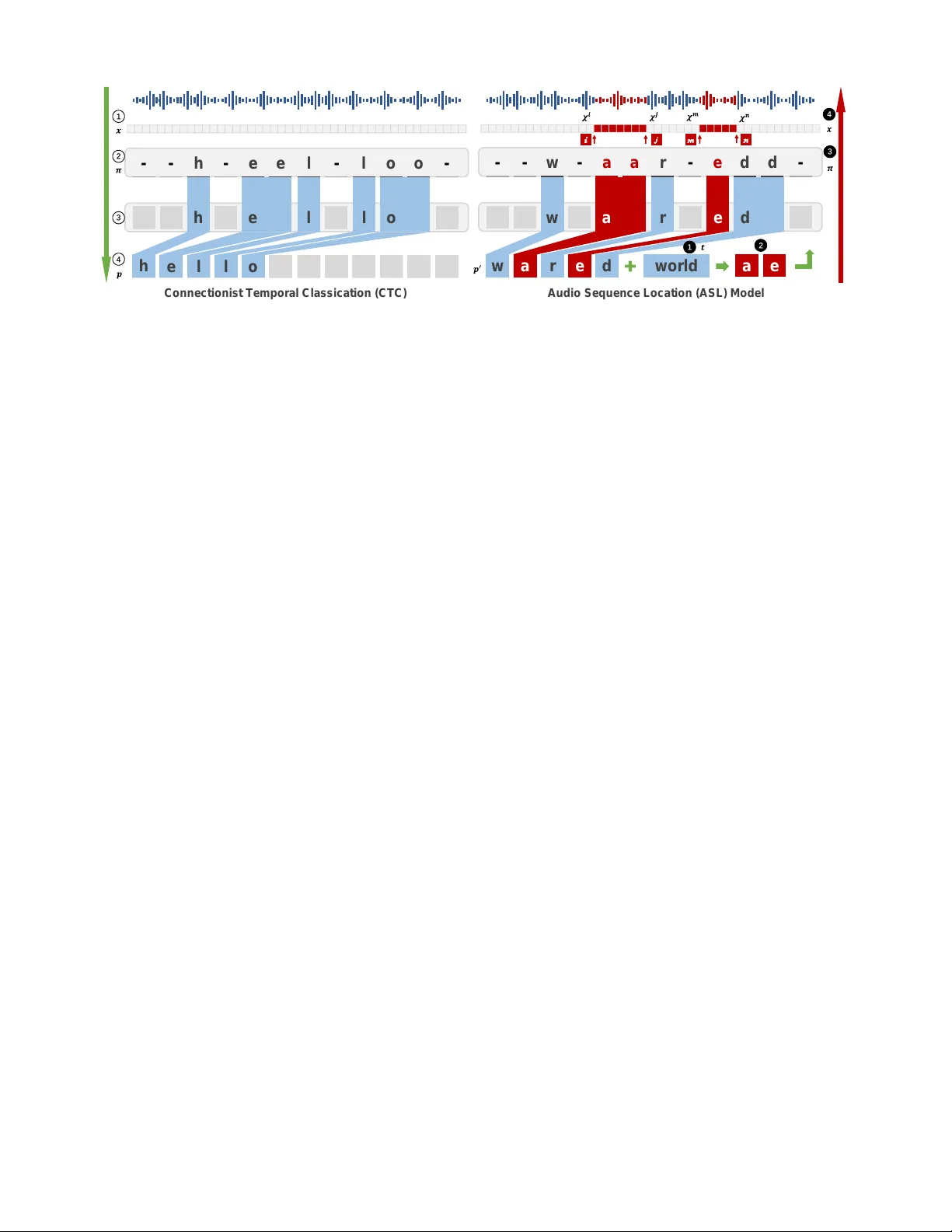
W eighted-Sampling A udio Adversarial Example Attack Xiaolei Liu, 1 Kun W an, 2 Y ufei Ding, 2 Xiaosong Zhang, 1 ∗ Qingxin Zhu 1 1 Univ ersity of Electronic Science and T echnology of China, 2 Univ ersity of California, Santa Barbara luxaole@gmail.com, { kun,yufeiding } @cs.ucsb .edu, { johnsonzxs,qxzhu } @uestc.edu.cn Abstract Recent studies hav e highlighted audio adversarial examples as a ubiquitous threat to state-of-the-art automatic speech recognition systems. Thorough studies on how to effecti vely generate adversarial examples are essential to pre vent poten- tial attacks. Despite many research on this, the ef ficiency and the robustness of existing works are not yet satisfactory . In this paper , we propose weighted-sampling audio adversarial examples , focusing on the numbers and the weights of dis- tortion to reinforce the attack. Further, we apply a denoising method in the loss function to make the adversarial attack more imperceptible. Experiments show that our method is the first in the field to generate audio adversarial examples with low noise and high audio robustness at the minute time- consuming lev el 1 . Introduction In recent years, machine learning algorithms are widely used in various fields. Howe ver , studies sho w that exist- ing learning-based algorithms are vulnerable to adversar - ial attacks (Szegedy et al. 2013; Goodfellow , Shlens, and Szegedy 2014). Currently , majority of the research on adv er- sarial examples are in the image recognition field (Kurakin, Goodfellow , and Bengio 2016; Carlini and W agner 2017; Chen et al. 2018; Su, V argas, and Sakurai 2019), while oth- ers in vestigate fields such as te xt classification (Jia and Liang 2017), traffic classification (Liu et al. 2018), and malicious software classification (Grosse et al. 2016; Hu and T an 2017; Liu et al. 2019). Automatic speech recognition (ASR) is another vital field where machine learning algorithms are also frequently ap- plied (Hinton et al. 2012). T o date, it has been proved that audio adv ersarial examples can mislead ASR to transfer any audio to an y tar geted phrases (Carlini and W agner 2018). ∗ Correspondence author is Xiaosong Zhang. This research was supported by National Ke y R&D Program of China (2017YFB0802900), National Natural Science Foundation of China (61572115,61902262), Sichuan Science and T echnology Program (2019JDRC0069). Copyright c  2020. 1 W e encourage you to listen to these audio adversarial e xamples on this website: https://sites.google.com/view/audio- adversarial- examples/. Howe ver , it is much more difficult to generate adversarial examples for audio than images. T o generate an effecti ve audio adversarial example, there are still sev eral technical challenges to be addressed: (C1) Generating audio adversarial examples demands sig- nificant computational resources and huge time overhead. It takes ov er one hour or more to generate an effecti ve audio adversarial example by recently proposed approaches (Car- lini and W agner 2018; Kreuk et al. 2018; Y uan et al. 2018; Qin et al. 2019). Such inefficiency significantly undermines the practicability of the attack. (C2) Recording and replaying, which are common oper- ations for audio, could easily introduce extra noise. There- fore, the robustness of adv ersarial e xamples against noise is crucial. Nev ertheless, the adversarial examples prepared ov er hours are still poor in robustness. The state-of-the- art audio adversarial examples (Carlini and W agner 2018; Alzantot, Balaji, and Sriv astav a 2018) become in valid after adding imperceptible pointwise random noise. (C3) Different from the image domain where l p -based metrics are carefully studied as a part of the loss function to generate adv ersarial examples, there are no in vestigations on which kind of metric is more suitable for constructing audio adversarial e xamples. In this paper , we achieve a fast, robust adversarial exam- ple attack to ASR by proposing tw o no vel techniques named W eighted Perturbation T echnology (WPT) and Sampling Perturbation T echnology (SPT) . WPT adjusts the weights of distortion at different posi- tions of audio during the generation process, and thus gen- erates adversarial examples faster and improves the attack efficienc y (addressing C1). Meanwhile, by reducing the number of points to perturb based on the characteristics of context correlation in the speech recognition model, SPT can increase the robustness of audio adversarial e xamples (addressing C2). T o best of our kno wledge, we are the first in the field to both take the factors of the weights and the numbers of perturbed points into consideration during the generation of audio adversarial examples. And the two techniques are al- ways complementary to all existing ASR adversarial attacks, which by default modify e very v alue of the entire audio vec- tor . Further , we also in vestigate different metrics as parts of the loss function to generate audio adversarial examples and provide a reference for future researchers in this field (ad- dressing C3). Finally , our experiments sho w that our method can gener - ate more r obust audio adversarial e xamples in a short period of 4 to 5 minutes . This is a substantial improv ement com- pared to the state-of-the-art methods. Related W ork Audio adv ersarial e xample attacks can be mainly di- vided into two categories, speech-to-label, and speech-to- text (Y ang et al. 2018). Speech-to-label classifies audio into different categories and the output is a specific label. This method is inspired by a similar method on images (Alzan- tot, Balaji, and Sri vasta va 2018; Cisse et al. 2017). Since the target phrases can only be chosen from a certain amount of labels, the practicality of such a method is limited. The speech-to-text method directly conv erts audio seman- tic information into text. Carlini & W agner (Carlini and W agner 2018) are the first to work on audio adversarial ex- amples for the speech-to-text models and they can let ASR transcribe any audio into a pre-specified text. Howe ver , the audio robustness is compromised and most of their exam- ples will lose the adversarial labels by adding imperceptible random noise. Later on CommanderSong (Y uan et al. 2018) achie ved practical over -the-air audio adversarial attacks, but they only validated their method on the music clips. Additionally Y akura & Sakuma (Y akura and Sakuma 2018) proposed an- other physical-world attack method. Regardless, these two methods will introduce non-negligible noise to the origi- nal audio. Unfortunately , all of these methods w ould require sev eral hours to generate only one audio adversarial exam- ple, including the most recent work (Qin et al. 2019). T o the best of our knowledge, there is no method to gen- erate audio adversarial examples with low noise and high robustness at the minute lev el. Our proposed method can be applied with all these current methods to achie ve a trade-of f among quality , robustness and con vergence speed. Background Threat Model. Before digging into details of the audio ad- versarial example attack, an ASR model should be selected as the potential threat model. Following the common prac- tice in the field we summarize three basic requirements for it: • Its core component should be Recurrent Neural Networks (RNNs) such as LSTM (Hochreiter and Schmidhuber 1997), which is widely adopted in current ASR systems; • It is vulnerable to the state-of-the-art audio adversarial at- tack methods, and the corresponding results could be used as baselines in our experiments; • It has to be open-source and thus we can directly conduct white-box tests on it. Giv en requirements above, we choose the speech-to-text model, Deepspeech (Hannun et al. 2014), as our e xperimen- tal threat model, which is an open-source ASR with Con- nectionist T emporal Classification (CTC) method (Grav es et al. 2006) and LSTM as its main components. Notice that our approach can be also applied to other RNN-based ASR systems. Considering that there are many ways to con vert the black-box model to a white-box model (Papernot, Mc- Daniel, and Goodfellow 2016; Oh et al. 2017; Ilyas et al. 2018), which is another research direction, and most of the previous work also assume they know the parameters of models, hence our research is also based on the white-box model. Au t o m a t i c S p e e c h R e c o g n i t i o n M od e l CT C L o ss F u n c t i o n g r ed i en t d escen t    A d v ers a r i a l ex a m p l e Figure 1: General process of audio adversarial example at- tack. A udio Adversarial Examples. Figure 1 shows the gen- eral process of audio adversarial e xample attack. Specifi- cally , let x be the input audio vector and δ is the distortion to the original audio. Audio adversarial example attacks are defined as by adding some perturbations δ , ASR recognizes x + δ as specified malicious te xts t (formally: f ( x + δ ) = t ), while there is no perceiv able difference for humans. The pro- cess of generating adversarial e xamples can be regarded as a process of updating x using gradient descent on a predefined loss function ` ( · ) shown in Eq. 1. The iterative process stops until the adversarial example meets our ev aluation require- ments. ` ( x, δ, t ) = ` model ( f ( x + δ ) , t ) + c · ` metric ( x, x + δ ) (1) In Eq. 1, ` model is the loss function used in the ASR models. For example, Carlini & W agner (Carlini and W agner 2018) uses CTC-loss as the ` model . ` metric is used to measure the difference between the generated adversarial examples and the original samples. Different from the image domain where l p -based metrics are commonly used, there is no con- sensus on which ` metric should be applied in the audio field. For instance, so f ar v arious ` metric such as SNR (Y uan et al. 2018), psychoacoustic hearing thresholds (Sch ¨ onherr et al. 2018) and frequency masking (Qin et al. 2019) have been adopted. W e will also elaborate the choices of l metric in this paper . Evaluation Metric. Based on the characteristics of the audio and the common practice in the field, the following ev aluation metrics are chosen in this paper . • SNR (Signal-to-noise ratio) measures the noise level of the distortion δ relativ e to the original audio x . The smaller distortion is, the larger SNR will be, SNR = 10 log 10 P x P δ , (2) where P x and P δ represent the ener gies of the original audio and the noise respectiv ely . • WER , i.e., the word error rate, is a common ev aluation metric in the ASR domain, WER = S + D + I N × 100% , (3) where S, D and I are the numbers of substitutions, dele- tions and insertions respectiv ely , and N is the total number of words. • Success Rate is the ratio of examples which can be suc- cessfully recognized as the malicious tar get texts by ASR, Success Rate = N adv N total × 100% , (4) where N adv is the number of adversarial examples that can be transcribed as target phrases and N total is the total number of adversarial e xamples generated. • Robustness Rate . Adding noise to the audio x is the same as applying transformation function t ∼ T over the input x . Here we define the robustness rate as the success ratio of examples that can still retain adversarial property after transformed by t ( · ) , Robustness Rate = N t ( adv ) N total × 100% , (5) where N t ( adv ) is the number of adversarial examples that can still be transcribed as target phrases after transformed by t ( · ) . Methodology In this section, first, we will show the details of sampling perturbation technology and weighted perturbation technol- ogy . W e will also explain why these methods are able to in- crease the robustness of adv ersarial e xamples and accelerate the attack. Finally , we will in vestigate different metrics and try to find out an experiential standard to refer to, instead of directly using the l p -based metrics on the image domain. Sampling perturbation technology W e propose SPT to increase the robustness of audio adver - sarial examples. It works by reducing the number of per - turbed points. Here we will explain the reason why SPT works, taking the CTC loss as an example. Actually it’ s a general method for current audio adversarial attacks. W e use x denote an audio vector , p denotes a phrase which is the semantic information of x and y denotes the probabil- ity distribution of x decoded to p . x i is one frame of x and y i is the probability distribution over the character which is transformed by x i . In CTC process (sho wn in Figure 2 left), the process from x to p is: Input x (Step 1) and get the sequences of tokens π (Step 2). Then merge the repeated characters and drop ‘-’ tokens (Step 3). Output the predicted phrase p (Step 4). Because π is the sequence of tokens to x , we say the prob- ability of π under y is the product of the likelihoods of each y i π i . For a gi ven phrase p with respect to y , there will be a set of predicted sequences π ∈ Q ( p, y ) . Finally , we calculate Pr( p | y ) , the probability of phrase p under the distrib ution y , by summing the probability of each π in the set: Pr( p | y ) = X π ∈ Q ( p,y ) n Y i =0 y i π i (6) In traditional audio adv ersarial e xample attack, if we want to transcribe audio x to target t , we will add slight distortion on each π i to let t = arg max p Pr( p | y ) . Howe ver , we can also get the same result by fixing part of n − m Y j y j π j and perturbing the other part to let m Y k y k π k = m Y k y 0 k π 0 k , where y 0 k is the ne w probability distribution of perturbed π 0 k and y k π k 6 = y 0 k π 0 k : t = arg max p Pr( p | y ) = arg max p X π ∈ Q ( p,y ) n Y i =0 y i π i = arg max p X π 0 ∈ Q ( p,y 0 ) n − m Y j =0 y j π j m Y k =0 y 0 k π 0 k (7) Based on Formula 7, we can shorten the perturbed number of audio vector from n to m . Our ev aluations gi ve the support that m can be much smaller than n . Since most of the points in our adversarial examples are exactly the same as those in the original audio, this makes our adv ersarial e xamples sho w v ery similar properties to the original audio. Compared with the adversarial e xamples that all points are perturbed, en vironmental noise has a lower probability of affecting the SPT -based adversarial examples. Athalye et al. (Athalye et al. 2017) proposed the Expecta- tion Over T ransformation (EO T) algorithm to construct ad- versarial examples that are able to maintain the adversarial property ov er a chosen transformation distrib ution T . Unfor- tunately , the limitation of the EO T is that it only increases robustness under the same or similar T -distribution noise. W ithout the assumption of similar distribution, the adv ersar- ial property will be largely compromised. As a comparison, our method does not need to have prior knowledge regard- ing the distribution when generating adversarial examples, thus we could hav e better general robustness. Meanwhile, our method is complementary to EO T . W eighted perturbation technology WPT can reduce the time cost by adjusting the weights of distortion in a different position. W e first point out the limi- tations of traditional loss function ` ( · ) (Eq. 1) and then giv e our solution. (Again, we introduce WPT based on CTC se- quence loss and WPT is a general method and can be easily applied to attack other ASR systems.) Current Pr oblem. By analyzing the process of gener - ating audio adversarial examples, we found that the closer the currently transcribed phrase p 0 is to the target text t , the C on n e c t i on i s t T e mpora l C l a s s i c a t i on ( C TC ) Aud i o S e qu e nc e Loc a t i on (A S L) M od e l h - - - e e l - l o o - h e l l o h e l l o w - - - a a r - e d d - w a r e d w a r e d a m n e i j w o r ld 1 2 3 4 4 3 2 1 Figure 2: Overvie w of CTC and ASL. longer it takes. In order to divide this process into different stages, we introduce the Levenshtein Distance (Lev enshtein 1966), which is a string metric for measuring the minimum number of single-character edits (i.e. insertions, deletions or substitutions) required to change one string into the other . According to our statistics, the average percentage of time loss spent on the Levenshtein distance from 3 to 2, 2 to 1 and 1 to 0 are, respectively , 7.52%, 15.43%, and 32.16%. Their sum exceeds 55% of the generation time. The reason for spending a lot of time at these stages is that when Leven- shtein Distance is small, most of the current points no longer need to be perturbed, e xcept for those points which cause the Lev enshtein Distance not to be 0. W e name these points as key points. On the one hand, if we can gi ve these ke y points larger weights, the time spent at this stage will be reduced; on the other hand, if the global search step size can be reduced with the number of iterations, then we can avoid missing a more perfect adversarial example due to over perturbing. These two aspects will make the o verall speed be accelerated. Steps of WPT : Accordingly , we implement WPT in two steps. The first step focuses on shortening the time cost when Le venshtein Distance equals to 1 by increasing the weights of key points. Therefore, we need to know which points are key points. Audio Sequence Location(ASL) is a model to help us lo- cate these key points in the audio. As shown in Figure 2 (right), the inputs of ASL are current transcribed phrase p 0 and target t (Step 1). After comparing p 0 and t , we get the different characters (Step 2). Find the positions of these characters in the sequence of tokens π (Step 3). Output the intervals set χ k in audio vector x (Step 4). Finally , the distor- tion corresponding to these k positions in χ k are multiplied by weights ω . Our impro ved formulation of ` ( · ) is, ` ( x, δ, t ) = ` model ( f ( x + α · δ ) , t ) + c · ` metric ( x, x + δ ) , α i =  ω , if i ∈ χ k 1 , else , ω > 1 , (8) where α is a weights vector to δ , and if the vector subscript i belongs to the intervals set χ k , we giv e these key points bigger weights ω . Besides, when we shorten Lev enshtein Distance to 0, WPT goes to its second step to reduce the learning rate lr : lr ← β · lr, (9) where constant β satisfies β ∈ (0 , 1) . After updating l r , we can calculate the perturbations δ on each iteration: δ 0 = 0 , δ n +1 ← δ n − l r · sig n ( ∇ δ ` ( x, δ, t )) , (10) where ∇ δ ` ( x, δ, t ) is the gradient of ` with respect to δ . Advantages: Carlini&W agner try to set different weights to each character of the sequence of π to solve this problem (Carlini and W agner 2018). Actually it will cost prohibitiv e computation to find the most suitable weight for each char- acter . So, they hav e to get a feasible solution x 0 which is found by using the normal CTC-loss function first and then using their improv ed method based on x 0 . Howe ver , this is not a perfect solution to solve the problem mentioned before. There are three advantages to our WPT : 1. Their method has to find a feasible solution x 0 first, which means they can not shorten the time cost before gen- erating a successful adversarial example. This period time accounts for more than 55% of the total time. W e can use ASL at any iterations to get the key location intervals χ k without having to obtain x 0 first. Then we make con verge faster by adjusting the weight ω of δ . 2. WPT is effecti ve against both a greedy decoder and beam-search decoder (Grav es et al. 2006), which are two searching ways combined with CTC to obtain the alignment π , while their method is only effecti ve against greedy de- coder . The reasons are a) Instead of adjusting the weight of a single character or token, we adjust the weights of a continuous interv al on the audio v ector corresponding to the character . This distortion based on the continuous interval is effecti ve for beam-search decoder . b) WPT updates weights ω according to the current alignment π instead of a fixed π 0 . So our method won’ t be limited to the greedy decoder . 3. The learning rate l r , that gradually decreases as the dis- tortion δ is reduced, can help us a void the problem of e xces- siv e perturbations due to too long steps so that better adver- sarial examples can be found more quickly . T able 1: Evaluation of our adv ersarial attack with Commander Song and C&W’ s attack. Attack Approach T arget phrase Proportion ↓ Ef ficiency(s) ↓ Success Rate ↑ dB x ( δ ) ↑ ** SNR ↑ Our attack Random phrases * 75% 251 1 46.92 31.9 C&W’ s attack Random phrases * all points ≈ 3600 1 38 - ** CommanderSong echo open the front door all points 3600 1 - ** 17.2 okay google restart phone no w all points 4680 1 - ** 18.6 * As is selected in C&W’ s work: target phrase is chosen at random such that (a) the transcription is incorrect (b) it is theoretically possible to reach that target. ** dB x ( δ ) is a l ∞ metric defined by C&W (Carlini and W agner 2018). And‘-’ means no relev ant data was provided in their papers. ‘ ↑ ’ means the bigger the better . In vestigation of metrics As for ` metric , which is the other part of ` ( · ) , also plays an important role in the generation of adversarial audio. Dif fer- ent from the image domain where mainly l p -based metrics are used as ` metric , there is no study on which metric should be selected. The purpose of ` metric is to limit the difference between the adversarial examples and the original samples. There- fore, we introduce the T otal V ariation Denoising (TVD) to reduce the noise perturbed and let adversarial examples sound more like the original audio. TVD is based on the principle that signals with excessiv e and possibly spurious detail have high total variation and is mostly used in the pro- cess of noise remov al (Rudin, Osher, and Fatemi 1992). Af- ter the TVD process, we can remove most of the impulse in the adversarial examples and make the distortion more im- perceptible. The ` metric based on TVD can be calculated via the sum of closeness E ( δ ) and total variation V ( x + δ ) : ` tv d metric ( x, δ ) = E ( δ ) + γ · V ( x + δ ) = 1 n n X i =0 ( δ i ) 2 + γ · n − 1 X j =1 | ( x j +1 + δ j +1 ) − ( x j + δ j ) | , (11) where γ is a trade off adjusted of E ( δ ) and V ( x + δ ) . Be- sides, we also in vestigate other three types of similarity met- rics which are selected in terms of 1) l ∞ in image domain; 2) l 2 -based in current audio domain; and 3) cosine distance in information retriev al domain; as shown in Formula 12. ` 1 metric ( x, δ ) = l ∞ ( x, x + δ ) ` 2 metric ( x, δ ) = l 2 ( x, x + δ ) ` 3 metric ( x, δ ) = (1 − cor ( x, x + δ )) , (12) where l ∞ ( · ) , l 2 ( · ) and cor ( · ) are, respectively , the measure- ment of l ∞ distance, l 2 distance and cosine distance between two audio vectors. A good choice of ` metric not only accurately reflects the auditory difference between the two audio frequencies but also a voids the optimization process oscillating around a so- lution without con ver ging (Carlini and W agner 2017). W e will giv e a comparison of the effects of various loss func- tions in the experimental section. Experimental results In this section, we sho w the e valuation of our adversarial attack used the technologies introduced in the Methodology Section. W e also study the performance of different ` metric on success rate, SNR and dB x ( δ ) . Our experimental results show that our approach has faster generation speed, better SNR, higher success rate, and stronger robustness than other attacks. Dataset and experimental settings Dataset. Mozilla Common V oice dataset 2 (MCVD): MCVD is an open and publicly a vailable dataset of voices that e very- one can use to train speech-enabled applications. It consists of voice samples require at least 70GB of free disk space. W e follo w the con vention in the field and use the first 100 test instances of this dataset to generate audio adversarial examples. Unless otherwise specified, all our experimen- tal results ar e av eraged over these 100 instances. En vironment. All experiments are carried out on an Ubuntu Server (16.04.1) with an Intel(R) Xeon(R) CPU E5- 2603 @ 1.70GHz, 16G Memory and GTX 1080 T i GPU. Experiments Evaluating adversarial examples In order to illustrate the effecti veness of our approach, we compared it with other two methods, Carlini & W agner’ s attack (Carlini and W ag- ner 2018) and CommanderSong (Y uan et al. 2018). T able 1 giv es the success probability , av erage SNR, dB x ( δ ) and ef- ficiency for our method and two other state-of-the-art meth- ods. For our method, we use SPT and WPT to improve the generation, use Eq. 7 as ` model and set ` tv d metric as our ` metric (Eq. 11), and the proportion of perturbed points is chosen to be 75%. As shown in T able 1, our fast approach shortens the gener- ation time from one hour to less than 5 minutes by focusing on the ke y points and dynamic learning rate to accelerate the con ver ge. In addition, our adversarial examples also have a better av erage of dB x ( δ ) and SNR, that is, we use less cal- culation time and get better results. More importantly , our approach has better robustness which is sho wn in the next section. 2 https://voice.mozilla.or g/en/datasets T able 2: The robustness against noise from 4 = 5 to 4 = 30 . Approach 4 = 5 4 = 15 4 = 30 Robustness ↑ WER ↓ Rob ustness ↑ WER ↓ Rob ustness ↑ WER ↓ baseline (C&W’ s attack) 0.23 0.49 0.04 0.81 0.01 0.93 EO T -based ( 4 = 5 ) 0.25 0.46 0.06 0.74 0.02 0.94 EO T -based ( 4 = 15 ) 0.63 0.16 0.07 0.56 0.02 0.92 EO T -based ( 4 = 30 ) 0.74 0.04 0.29 0.23 0.04 0.70 SPT -based (proportion =5%) 0.71 0.04 0.4 0.22 0.27 0.39 SPT -based (proportion =30%) 0.58 0.15 0.21 0.33 0.11 0.58 SPT -based (proportion =75%) 0.42 0.21 0.18 0.50 0.06 0.72 SPT -EO T -based (75%,30) 0.85 0.03 0.30 0.19 0.09 0.53 T able 3: Evaluation of dif ferent loss functions in our adversarial attacks. Loss functions * SNR ↑ dB x ( δ ) ↑ Success Rate ↑ ` 0 = ` model + c 0 · ` tv d metric 31.9 46.92 1 ` 1 = ` model + c 1 · ` 1 metric 29.17 44.55 0.97 ` 2 = ` model + c 2 · ` 2 metric 30.2 44.91 1 ` 3 = ` model + c 3 · ` 3 metric 30.1 44.63 0.98 * W e tried our best to tune every constant c of different ` metric for a fair comparison. W e refer interested readers to Implementation Details Section for setting details. Evaluating r obustness to noise As we mentioned in Eq.5, we e valuate the robustness of audio adv ersarial examples by adding noise to them and checking their adversarial proper- ties. The process of adding noise is equal to apply transfor- mation function t ∼ T over the input audio. In our experi- ments, we set T as the uniform distribution with the bound- ary of ±4 . W e respectively added noise to SPT -based, EO T - based and SPT -EO T -based adversarial examples. Then we transcribed the newly obtained audio and finally calculate WER and Robustness Rate. If the newly transcribed phrase is the same as before, we say that this audio successfully bypassed the noise defense. As shown in T able 2, mostly the SPT -based method per- forms better than the EOT -based method in terms of WER. The EOT -based audio has a higher Robustness Rate when its distribution is the same or similar to the noise distribution. Howe ver , the SPT -based audio exhibits more general robust- ness. More specifically , in SPT , the smaller the proportion, the better the robustness, but too small proportion results in a decrease in SNR and success rate. Fortunately , the SPT - EO T -based approach combines the advantages of both meth- ods and performs well in all aspects. W e recommend using the SPT -EO T -based approach to increase robustness in fu- ture work. In vestigation of different ` metric In this experiment, we generate adversarial e xamples based on ` model and four dif- ferent ` metric (from Eq. 11 to Eq. 12). For each specific loss function, we conduct adversarial attacks both with SPT (un- der the proportion of 75%) and WPT . The results in T able-3 suggest that ` 0 has the best perfor- mance on SNR, dB x ( θ ) and success rate. Besides, because the TVD process eliminates the harsher impulse noise, the added perturbation ”sounds” more imperceptible. As a re- sult, although the SNR and dB x ( θ ) of ` 0 are not greatly im- prov ed in numerical v alue, its adversarial audio sounds quite better . Here we again suggest you listen to our demos on the website has giv en before. The overall performances of ` 1 and ` 3 are not satisf actory . Since the maximum value in the audio vector is impossible to measure the magnitude of the two small disturbances un- der the same maximum value. It also proves that the charac- ter of the cosine distance is more suitable for audio similarity measurement. Because l 2 distance can reflect all the pertur- bation of audio, ` 2 has a better performance than ` 1 and ` 3 , especially on the success rate. Howe ver , it’ s still worse than ` 0 on SNR and dB x ( θ ) . Combined the experimental results and the process of tun- ing, we conclude that a good loss function should satisfy the following three characteristics: 1) The value ranges of ` model and c · ` metric should be the same order of magni- tude; 2) It should ensure that the value of ` model are rela- tiv ely larger in the initial stage, so that a feasible solution can be found as soon as possible; after finding a feasible solution, the weight of `metr ic should increase, because it is necessary to find a feasible solution that is closer to the original sample; 3) Considering the characteristic of sound, a metric in audio area instead of general metric can lead to a more imperceptible adversarial audio. Implementation Details For reproducibility , here we giv e the hyperparameters used in our experiments. Evaluating adversarial examples In this experiment, we generate audio adversarial examples with SPT and WPT and we select ` tv d metric as ` metric . The searching decoder is a beam-search decoder . The max iteration is set to be 500, which is enough for our method to generate imperceptible adversarial examples. In SPT , the proportion of perturbed points is 75%. In WPT , we set the weights of key points to be 1.2, the learning rate begins with 100 and β is set to be 0.8. l r will be updated by β · lr , if the iterations %50 == 0 and we have generated at least one adversarial example by now . The hyperparameters c and γ are 0.001 and 10. Evaluating rob ustness to noise Most of the hyperparam- eters are set to be the same as the first experiment except that the proportion of perturbed points are 5%, 15%, 30%, 75%, respectiv ely . In vestigation of different l metric Most of hyperparame- ters are set to be the same as the first experiment. And c 1 , c 2 , c 3 are 0.01, 0.001, 1, respectiv ely . T ranscription Examples Some of the transcription examples are shown in T able 4. All of the phrases are selected randomly from the MCVD. T able 4: Some of the transcription examples. Original phrase 1 he thought of all the married shep- herds he had known T argeted phrase 1 we’ re refugees from the tribal wars and we need money the other fig- ure said Original phrase 2 i told him we could teach her to ig- nore people who waste her time T argeted phrase 2 down below in the darkness were hundreds of people sleeping in peace Original phrase 3 but finally the merchant appeared and asked the boy to shear four sheep T argeted phrase 3 it seemed so safe and tranquil Original phrase 4 this is no place for you T argeted phrase 4 but finally the merchant appeared and asked the boy to shear four sheep Original phrase 5 some of the grey ash was falling off the circular edge T argeted phrase 5 we’ re refugees from the tribal wars and we need money the other fig- ure said Notations and Definitions All notations and definitions used in our paper are listed in T able 5. Conclusion This paper proposes a weighted-sampling audio adversar- ial example attack. The experimental results sho w that our method has faster speed, less noise, and stronger rob ustness. More importantly , we are the first to introduce the factor of the numbers and weights of perturbed points into the gener- ation of audio adversarial examples. W e also introduce TVD T able 5: Notations and Definitions used in our paper . x The original input audio δ The distortion to the original audio t The targeted te xts f ( · ) The threat model ` ( · ) The loss function to generate audio adver- sarial examples ` model ( · ) The loss function to measure the dif ference between the current output of the model and the targeted te xts ` metric ( · ) The loss function to limit the difference between the adversarial examples and the original samples p The phrase of the semantic information of original audio p 0 The current transcribed phrase by ASL y The probability distribution ov er the trans- formed characters π The sequence of tokens n The length of the original audio vector m The length of the perturbed audio v ector χ the key location interv al set c A hyperparameter to balance the impor- tance of ` model and ` metric ω The weights of key points α The weights of δ lr The learning rate in gradient descent β A h yperparameter to control the rate of de- crease of the learning rate ∇ δ ` ( · ) The gradient of ` ( · ) with regard to δ E ( · ) The sum of closeness V ( · ) The total v ariation γ A hyperparameter to balance the impor- tance of E ( · ) and V ( · ) l p ( · ) The l p distance, such as l 0 , l 2 , and l ∞ etc. cor ( · ) The cosine distance to improv e the loss function. The study of the effecti veness of loss function shows there are some differences between the adversarial examples of image and audio. It also guides us on how to construct a more appropriate loss function in the future. Our future work will focus on the defense of au- dio adversarial e xamples. References [Alzantot, Balaji, and Sriv astav a 2018] Alzantot, M.; Balaji, B.; and Sriv astav a, M. 2018. Did you hear that? adversar- ial examples against automatic speech recognition. arXiv pr eprint arXiv:1801.00554 . [Athalye et al. 2017] Athalye, A.; Engstrom, L.; Ilyas, A.; and Kwok, K. 2017. Synthesizing robust adversarial ex- amples. arXiv preprint . [Carlini and W agner 2017] Carlini, N., and W agner , D. 2017. T owards ev aluating the robustness of neural networks. In 2017 IEEE Symposium on Security and Privacy (SP) , 39– 57. IEEE. [Carlini and W agner 2018] Carlini, N., and W agner , D. 2018. Audio adversarial examples: T argeted attacks on speech-to- text. In 2018 IEEE Security and Privacy W orkshops (SPW) , 1–7. IEEE. [Chen et al. 2018] Chen, P .-Y .; Sharma, Y .; Zhang, H.; Y i, J.; and Hsieh, C.-J. 2018. Ead: elastic-net attacks to deep neural networks via adversarial examples. In Thirty-Second AAAI Confer ence on Artificial Intelligence . [Cisse et al. 2017] Cisse, M.; Adi, Y .; Nev erov a, N.; and Keshet, J. 2017. Houdini: Fooling deep structured prediction models. arXiv preprint . [Goodfellow , Shlens, and Szegedy 2014] Goodfellow , I. J.; Shlens, J.; and Szegedy , C. 2014. Explaining and harnessing adversarial e xamples. arXiv pr eprint arXiv:1412.6572 . [Grav es et al. 2006] Graves, A.; Fern ´ andez, S.; Gomez, F .; and Schmidhuber , J. 2006. Connectionist temporal classifi- cation: labelling unsegmented sequence data with recurrent neural networks. In Pr oceedings of the 23rd international confer ence on Machine learning , 369–376. A CM. [Grosse et al. 2016] Grosse, K.; Papernot, N.; Manoharan, P .; Backes, M.; and McDaniel, P . 2016. Adversarial perturba- tions against deep neural networks for malware classifica- tion. arXiv preprint . [Hannun et al. 2014] Hannun, A.; Case, C.; Casper , J.; Catanzaro, B.; Diamos, G.; Elsen, E.; Prenger , R.; Satheesh, S.; Sengupta, S.; Coates, A.; et al. 2014. Deep speech: Scaling up end-to-end speech recognition. arXiv preprint arXiv:1412.5567 . [Hinton et al. 2012] Hinton, G.; Deng, L.; Y u, D.; Dahl, G. E.; Mohamed, A.-r .; Jaitly , N.; Senior, A.; V anhoucke, V .; Nguyen, P .; Sainath, T . N.; et al. 2012. Deep neural networks for acoustic modeling in speech recognition: The shared views of four research groups. IEEE Signal pr ocess- ing magazine 29(6):82–97. [Hochreiter and Schmidhuber 1997] Hochreiter , S., and Schmidhuber , J. 1997. Long short-term memory . Neural computation 9(8):1735–1780. [Hu and T an 2017] Hu, W ., and T an, Y . 2017. Generating adversarial malware examples for black-box attacks based on gan. arXiv pr eprint arXiv:1702.05983 . [Ilyas et al. 2018] Ilyas, A.; Engstrom, L.; Athalye, A.; and Lin, J. 2018. Black-box adv ersarial attacks with limited queries and information. arXiv preprint . [Jia and Liang 2017] Jia, R., and Liang, P . 2017. Adversar - ial e xamples for ev aluating reading comprehension systems. arXiv pr eprint arXiv:1707.07328 . [Kreuk et al. 2018] Kreuk, F .; Adi, Y .; Cisse, M.; and K eshet, J. 2018. Fooling end-to-end speaker v erification with adver - sarial examples. In 2018 IEEE International Conference on Acoustics, Speech and Signal Pr ocessing (ICASSP) , 1962– 1966. IEEE. [Kurakin, Goodfello w , and Bengio 2016] Kurakin, A.; Goodfellow , I.; and Bengio, S. 2016. Adversarial examples in the physical world. arXiv pr eprint arXiv:1607.02533 . [Lev enshtein 1966] Lev enshtein, V . I. 1966. Binary codes capable of correcting deletions, insertions, and reversals. In Soviet physics doklady , v olume 10, 707–710. [Liu et al. 2018] Liu, X.; Zhang, X.; Guizani, N.; Lu, J.; Zhu, Q.; and Du, X. 2018. Tltd: a testing frame work for learning- based iot traffic detection systems. Sensors 18(8):2630. [Liu et al. 2019] Liu, X.; Du, X.; Zhang, X.; Zhu, Q.; W ang, H.; and Guizani, M. 2019. Adv ersarial samples on an- droid malware detection systems for iot systems. Sensors 19(4):974. [Oh et al. 2017] Oh, S. J.; Augustin, M.; Schiele, B.; and Fritz, M. 2017. T owards re verse-engineering black-box neu- ral networks. arXiv pr eprint arXiv:1711.01768 . [Papernot, McDaniel, and Goodfello w 2016] Papernot, N.; McDaniel, P .; and Goodfello w , I. 2016. T ransferability in machine learning: from phenomena to black-box attacks us- ing adversarial samples. arXiv pr eprint arXiv:1605.07277 . [Qin et al. 2019] Qin, Y .; Carlini, N.; Goodfello w , I.; Cot- trell, G.; and Raffel, C. 2019. Imperceptible, robust, and targeted adversarial examples for automatic speech recogni- tion. arXiv preprint . [Rudin, Osher , and Fatemi 1992] Rudin, L. I.; Osher , S.; and Fatemi, E. 1992. Nonlinear total variation based noise re- mov al algorithms. Physica D: nonlinear phenomena 60(1- 4):259–268. [Sch ¨ onherr et al. 2018] Sch ¨ onherr , L.; K ohls, K.; Zeiler , S.; Holz, T .; and Kolossa, D. 2018. Adversarial attacks against automatic speech recognition systems via psychoacoustic hiding. arXiv preprint . [Su, V argas, and Sakurai 2019] Su, J.; V argas, D. V .; and Sakurai, K. 2019. One pixel attack for fooling deep neural networks. IEEE T ransactions on Evolutionary Computation . [Szegedy et al. 2013] Szegedy , C.; Zaremba, W .; Sutske ver , I.; Bruna, J.; Erhan, D.; Goodfello w , I.; and Fergus, R. 2013. Intriguing properties of neural networks. arXiv preprint arXiv:1312.6199 . [Y akura and Sakuma 2018] Y akura, H., and Sakuma, J. 2018. Robust audio adversarial example for a physical at- tack. arXiv preprint . [Y ang et al. 2018] Y ang, Z.; Li, B.; Chen, P .-Y .; and Song, D. 2018. Characterizing audio adversarial examples using temporal dependency . arXiv pr eprint arXiv:1809.10875 . [Y uan et al. 2018] Y uan, X.; Chen, Y .; Zhao, Y .; Long, Y .; Liu, X.; Chen, K.; Zhang, S.; Huang, H.; W ang, X.; and Gunter , C. A. 2018. Commandersong: A systematic ap- proach for practical adversarial voice recognition. In 27th { USENIX } Security Symposium ( { USENIX } Security 18) , 49–64.