Grace periods in comparative effectiveness studies of sustained treatments

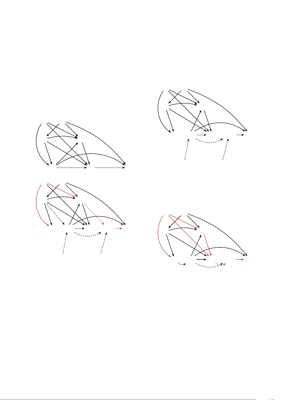
Grace p erio ds in comparativ e eﬀectiv eness studies of sustained treatmen ts Kerollos Nashat W anis a,b, ∗ , Aaron L. Sarv et c , Lan W en d , Jason P . Blo c k e , Sheryl L. Rifas-Shiman e , James M. Robins a,f , Jessica G. Y oung a,e a Dep artment of Epidemiolo gy, Harvar d T. H. Chan Scho ol of Public He alth, Boston, Massachusetts, USA b Dep artment of Br e ast Sur gic al Onc olo gy, MD A nderson Canc er Center, Houston, TX, USA c Dep artment of Mathematics, ´ Ec ole Polyte chnique F ´ ed´ er ale de L ausanne, Switzerland d Dep artment of Statistics and A ctuarial Scienc e, University of Waterlo o, Waterlo o, Ontario, Canada e Dep artment of Population Me dicine, Harvar d Me dic al Scho ol and Harvar d Pilgrim He alth Car e Institute, Boston, Massachusetts, USA f Dep artment of Biostatistics, Harvar d T.H. Chan Scho ol of Public He alth, Boston, Massachusetts, USA Abstract Researc hers are often in terested in estimating the eﬀect of sustained use of a treatment on a health outcome. Ho wev er, adherence to strict treatment proto cols can b e challenging for individuals in practice and, when non-adherence is expected, estimates of the eﬀect of sustained use ma y not b e useful for decision making. As an alternativ e, more relaxed treatmen t proto cols whic h allow for p erio ds of time oﬀ treatment (i.e., grace p erio ds) ha ve b een considered in pragmatic randomized trials and observ ational studies. In this pap er w e consider the in terpretation, identiﬁcation, and estimation of treatmen t strategies whic h include grace p erio ds. W e contrast natur al grace p erio d strategies whic h allo w individuals the ﬂexibilit y to tak e treatmen t as they w ould naturally do, with sto chastic grace p eriod strategies in whic h the in vestigator sp eciﬁes the distribution of treatmen t utilization. W e estimate the eﬀect of initiation of a thiazide diuretic or an angiotensin-con v erting enzyme inhibitor in h yp ertensiv e individuals under v arious strategies whic h include grace p erio ds. R unning he ad: Grace p eriods for comparative eﬀectiv eness ∗ Con tact information for corresponding author: Kerollos N. W anis, Departmen t of Breast Surgical Oncology , MD Anderson Cancer Center, 1400 Pressler St, Unit 1434—F CT7.6088, Houston, TX, USA. knwanis@gmail.com 1. In tro duction Man y randomized and observ ational studies aim to compare the safet y and/or eﬃcacy of diﬀeren t treatmen ts indicated for the same disease diagnosis. These c omp ar ative eﬀe ctive- ness studies ha v e formed the basis for v arious pharmacologic recommendations in medical guidelines. American Heart Asso ciation (AHA) guidelines are one example. The AHA equiv alen tly supp ort either thiazide diuretics or angiotensin-con verting enzyme inhibitors (A CEIs) as ﬁrst-line treatmen t for hypertension ( Whelton et al. , 2018 ). A Co c hrane review mainly based on randomized trials prior to the y ear 2000 informs the AHA recommenda- tions, but ackno wledges that evidence for ACEI eﬀectiv eness is of lo w qualit y ( Musini et al. , 2017 ). A recent large scale observ ational study comparing initiation of v arious antih yp er- tensiv e agents found that thiazides hav e b etter primary eﬀectiv eness than A CEIs ( Suchard et al. , 2019 ). In comparativ e eﬀectiv eness studies, inv estigators migh t express in terest in causal eﬀects of sustained use, e.g., the eﬀect on cardiov ascular outcomes of taking a thiazide diuretic medication (v ersus an A CEI medication) con tinuously o ver the follow-up. Ho wev er, it can be unrealistic to exp ect study participan ts to adhere to a strict treatmen t strategy (also termed a proto col or a regime) that demands con tin uous utilization of treatment. In causal inference, suc h strict proto cols are examples of time-v arying static deterministic treatmen t strategies: treatmen t rules requiring the same v alue of treatment for all individuals at a given time during the follow-up ( Hern´ an and Robins , 2020 ; Robins and Hern´ an , 2009 ). Deterministic strategies can b e made more realistic b y allo wing cessation of treatment when unmanageable treatmen t-related toxicities o ccur ( Hern´ an et al. , 2017 ; Robins and Fink elstein , 2000 ). Adherence to strict deterministic rules is often c hallenging for individuals in practice, with adherent individuals often representing a small prop ortion of the study p opulation. In terruptions in utilization of even greater than 60 da ys ha ve b een observed in one-third to one-half of individuals who initiate antih yp ertensiv es, with interruptions b eing more com- 2 mon in those using thiazides ( Elliott et al. , 2007 ). This can translate to (near) positivity violations ( Petersen et al. , 2012 ; Kennedy , 2019 ; Robins , 1986 ), which can preclude consis- ten t estimation of eﬀects of con tinuous utilization. Arguably , these p ositivit y concerns also reﬂect the limited real-w orld clinical relev ance of strict deterministic treatment strategies. As a pragmatic alternative, more relaxed study proto cols hav e b een deﬁned in randomized trials to b etter reﬂect actual clinical practice ( So x and Lewis , 2016 ; Loudon et al. , 2015 ), allo wing for delays in treatmen t initiation or for p erio ds of time oﬀ treatmen t after initiation, ev en in the absence of toxicities or other severe clinical ev en ts ( F ord and Norrie , 2016 ). These allow ances can b e put into practice using gr ac e p erio ds - perio ds of time in whic h breaks from sustained use of treatmen t are permitted under the proto col. T reatment proto- cols in pragmatic trials allo wing grace p erio ds t ypically sp ecify that individuals take treat- men t as they w ould naturally until the end of the grace perio d, at which time they m ust tak e treatmen t if they ha ve not already done so. Causal eﬀects of suc h natur al gr ac e p erio d str ate gies hav e also been considered in observ ational studies, typically with a single grace p eriod prior to treatment initiation ( Y oung et al. , 2011 ; Cain et al. , 2010 ; Huitfeldt et al. , 2015 ; Hern´ an and Robins , 2016 ). Ho wev er, the relative eﬀectiv eness of tw o medications is diﬃcult to interpret under natu- ral grace p eriod strategies. Ev en if the medications hav e iden tical ‘pharmacological’ eﬃcacy , their eﬀectiv eness under natural grace p erio d strategies ma y diﬀer substan tially if natural utilization of the drugs diﬀers during grace p eriods. Motiv ated by a study using data from Kaiser Permanen te Colorado (KPC) comparing an tihypertensive monotherapies, we will elab orate on the interpretation of eﬀects under treatmen t strategies which include grace p erio ds. As a compromise b etw een strict proto cols requiring contin uous treatment utilization and natural grace p eriod proto cols, we describ e alternativ e grace p erio d proto cols which are a ﬂexible set of treatmen t strategies that can mitigate the highligh ted issues inherent in the aforemen tioned extremes. W e refer to this 3 class of rules as sto chastic grace perio d strategies. W e consider assumptions needed for iden tiﬁcation of risk under this class of rules and how to reason ab out them under sub ject matter kno wledge using Single W orld In terv ention Graphs (SWIGs) ( Richardson and Robins , 2013b ). W e implemen t an estimator based on the eﬃcien t inﬂuence function, which p ermits the use of ﬂexible mac hine learning algorithms for confounding adjustment. 2. Observ ed data W e consider a longitudinal study in which time-v arying measurements are a v ailable for a random sample of N individuals from a target p opulation who are indicated to initiate one of tw o antih yp ertensiv es. Let Z denote the medication initiated, with Z = 1 denoting initiation of a thiazide diuretic and Z = 0 an ACEI. T o a void distracting from cen tral issues, w e assume no loss to follo w-up until Supplementary Materials Section S9 , and, although w e consider a surviv al outcome in this man uscript, the results presen ted here can be generalized to settings with other t yp es of outcomes. After treatmen t initiation, suppose the follo wing naturally-arising cov ariates are mea- sured in discrete time interv als (e.g., days, mon ths), k = 1 , . . . , K , with k = 1, the interv al of treatment initiation (baseline), and k = K , the end of follow-up of in terest (e.g., 36 mon ths): a vector of cov ariates describing the individual’s status in in terv al k , L k (e.g., new disease diagnoses); an indicator of adherence to the initiated medication in in terv al k , A k ; and an indicator of failure (e.g., adverse cardiov ascular ev ents) b y the end of the interv al, Y k . L 1 ma y also include time-ﬁxed c haracteristics (e.g., age at baseline, sex, history of diab etes mellitus at baseline). In eac h in terv al, w e assume the temp oral ordering ( L k , A k , Y k ). Ov erlines are used to represen t an individual’s history of co v ariates, treatment, or outcome from interv al k (e.g., L k ). Individuals are outcome-free at the b eginning of the study ( Y 0 = 0), and, by notational con ven tion, L 0 and A 0 are set to an arbitrary constan t (e.g., 0). W e use low er-case letters 4 to denote p ossible realizations of random v ariables (e.g., a k is a realization of A k ). 3. Deﬁning causal eﬀects of treatment strategies with grace p erio ds Deﬁne Y z ,g m k as an individual’s failure status b y interv al k had, p ossibly contrary to fact, they follow ed a treatment strategy that ensures they initiate medication z and then subse- quen tly follow a particular time-v arying grace perio d strategy g m that allows m consecutive in terv als without adhering to that medication. W e can, in turn, quantify the comparative eﬀectiv eness of suc h strategies comparing diﬀerent lev els of z on the outcome risk by k as the coun terfactual risk contrast Pr[ Y 1 ,g m k = 1] vs. Pr[ Y 0 ,g m k = 1] . (1) In the sp ecial case of m = 0 (no grace p erio d), ( 1 ) captures the eﬀect of con tinuous utilization of the diﬀerent medications, i.e., Y z ,g 0 k = Y z ,a K =1 k . As suc h, static treatmen t regimes may alwa ys b e understo o d as a sp ecial case of a grace-p eriod regime. How ever, when m > 0, the eﬀect ( 1 ), and the absolute risk Pr[ Y z ,g m k = 1], ma y hav e any num b er of in terpretations dep ending on ho w the treatment rules deﬁning g m are c hosen. F ollo wing Richardson and Robins ( 2013b ), let A z ,g m k denote the natural v alue of treatment at k under a grace p erio d strategy indexed by z and m , and let A z ,g m + k denote the intervention v alue of treatmen t. A z ,g m k is the treatmen t lev el that w e w ould observ e if that strategy w ere implemen ted up to k but no interv en tion was made at k , while A z ,g m + k is the treatmen t level that w ould b e assigned at k under the treatment strategy . T o facilitate deﬁnition of grace p eriod strategies, deﬁne R z ,g m + k as the n um b er of consec- utiv e interv als of follow-up prior to k that an individual do es not adhere to treatmen t under a grace p erio d strategy indexed b y z , g m . Initializing, for k = 1, R z ,g m + 1 = 0, we recursiv ely 5 deﬁne R z ,g m + k : = ( R z ,g m + k − 1 + 1) × (1 − A z ,g m + k − 1 ) (2) k = 2 , . . . , K + 1. Therefore, R z ,g m + k is a deterministic function of the interv ention treatmen t history prior to k , counting consecutiv e in terv als without treatment adherence and resetting to 0 whenev er treatment is assigned in the prior interv al. Natural grace p erio d strategies hav e b een the implicit type of grace p erio d strategy in proto cols of pragmatic trials as well as in the em ulation of such trials with observ ational data ( Cain et al. , 2010 ; Y oung et al. , 2011 ). W e will now formally deﬁne these strategies, con- trasting them with a family of alternative strategies, sto c hastic grace p erio d strategies. The diﬀeren t nature of these deﬁnitions will hav e implications for interpretation of Pr[ Y z ,g m k = 1] and the eﬀect ( 1 ) but also for the assumptions needed for identiﬁcation of these coun terfac- tual quan tities with observed data. W e will discuss these assumptions in Section 5 . 3.1. Natur al gr ac e p erio d str ate gies Under a natural grace p erio d strategy , for individuals surviving to k (i.e., Y z ,g m k − 1 = 0), we deﬁne A z ,g m + k : =        A z ,g m k : R z ,g m + k < m, 1 : R z ,g m + k = m. (3) W e emphasize the distinctiv e feature of natural grace p erio d regimes: that A z ,g m + k := A z ,g m k whenev er R z ,g m + k < m . In words, surviving individuals will take treatmen t as they would natur al ly (no in terv ention will b e made) at times k that are during a grace perio d. Because in terven tion treatment v alues are equal to natural treatmen t v alues at all times during a grace p erio d (when R z ,g m + k < m ) under this rule, it follo ws by the deﬁnition of R z ,g m + k in ( 2 ) that treatmen t assignmen t at the end of a grace p eriod (when R z ,g m + k = m ) is a function of the natural treatmen t history . Therefore, a natural grace p erio d strategy is an interv ention 6 that dep ends on the natural treatmen t history . F or examples of other interv entions that dep end on the natural treatment history , see Richardson and Robins ( 2013b ); Y oung et al. ( 2014 ); Haneuse and Rotnitzky ( 2013 ); D ´ ıaz et al. ( 2021 ). Remark 1. In the sp e cial c ase of m > K , for a natur al gr ac e p erio d str ate gy, ( 1 ) is e quivalent to the eﬀe ct of initiating me dic ation then making no intervention on adher enc e at any time p oint (an analo gue of the ‘intention-to-tr e at’ eﬀe ct) sinc e R z ,g m + k < m at al l times k . 3.2. Sto chastic gr ac e p erio d str ate gies In con trast to a natural grace p erio d strategy , consider an alternative class of strategies indexed b y z , g m whic h we will generally deﬁne as follo ws: for those surviving under the strategy to k (i.e., Y z ,g m k − 1 = 0), let X k ∼ U (0 , 1) b e an exogenous randomly drawn v alue from a standard uniform distribution and, using an investigator -sp eciﬁed function π inv k , deﬁne A z ,g m + k : =                1 : R z ,g m + k < m and X k ≤ π inv k ( L z ,g m k , A z ,g m + k − 1 , z ) , 0 : R z ,g m + k < m and X k > π inv k ( L z ,g m k , A z ,g m + k − 1 , z ) , 1 : R z ,g m + k = m. (4) where L z ,g m k is the history of the v alues of the cov ariates at k under the strategy and π inv k giv es the probabilit y of receiving treatment during a grace p eriod, whic h ma y dep end on the cov ariate and interv ention treatmen t history ( L z ,g m k , A z ,g m + k − 1 ), as w ell as the medication initiated, z , under the strategy . When π inv k dep ends trivially on some of its argumen ts, we will omit those argumen ts from the function (e.g., as in Supplementary Materials Section S1 ). W e will refer to any strategy within the class ( 4 ) as a sto chastic grace p eriod strategy . In w ords, under a sto c hastic grace p erio d strategy , an in terven tion on treatment will o ccur at all times k that are during a grace p eriod – individuals will either b e forced to tak e treatmen t or not take treatment dep ending on the random draw of the exogenous random v ariable X k and the in vestigator c hosen treatmen t probabilit y π inv k . The c hoice of π inv k allo ws 7 in vestigators to control the amoun t and distribution of non-adherence allow ed under the grace p erio d treatmen t strategy . Inv estigators migh t c ho ose to induce a discrete analogue of a particular con tinuous distribution, as w e illustrate in Supplementary Materials Section S2 . Alternativ ely , a constant π inv k ma y b e a parsimonious c hoice. W e can see from the deﬁnition ( 4 ) that, unlik e a natural grace p erio d strategy , a sto c has- tic grace perio d strategy do es not dep end on the natural treatment history but, at most, is allo wed to dep end on the in terv ention treatment history , the co v ariate history , the initiated medication, and an exogenous randomizer. Recall, by deﬁnition ( 2 ), that R z ,g m + k is a func- tion of the in terven tion treatmen t history A z ,g m + k − 1 . Thus, an inv estigator migh t restrict the dep endence of the sto c hastic grace p eriod strategies as deﬁned in ( 4 ) to R z ,g m + k rather than the en tire interv ention treatmen t history . A sto c hastic grace p erio d strategy with m = 3 following initiation of an ACEI could b e implemen ted b y having in v estigators ﬂip a fair coin for each individual at the b eginning of eac h mon th. If the result of the coin ﬂip is heads, then the individual receiv es a month’s supply of ACEI. If the result is tails, then the individual do es not receiv e medication. Ho wev er, if an individual has gone 3 consecutive months without medication (due to prior coin ﬂips), then no coin ﬂip is necessary b ecause they m ust receiv e a disp ensation. This sto c hastic grace p erio d strategy dep ends only on R z ,g m + k , and sets π inv k = 0 . 5. By contrast, a natural grace p erio d strategy with m = 3 would allo w individuals to miss their monthly A CEI disp ensations ov er the course of follo w-up according to their natural inclinations so long as they never miss more than 3 in a ro w, at whic h point they would b e required to receiv e a disp ensation. The distribution of treatmen t adherence is therefore not under the con trol of the in v estigator when a natural grace perio d strategy is c hosen. In Supplemen tary Materials Section S1 and S3 w e consider other sp eciﬁc examples of grace p eriod strategies. 8 4. Implications of the c hoice of grace p erio d strategy for interpretation in com- parativ e eﬀectiveness researc h T o consider the implications of a particular choice of grace p eriod strategy on in terpreta- tion of the counterfactual absolute risk Pr[ Y z ,g m k = 1] and the eﬀect ( 1 ), we will consider our motiv ating study comparing antih yp ertensiv e agen ts under grace p erio d strategies. Supp ose that individuals initiate a medication from the A CEI class ( z = 0) or a medication from the thiazide diuretic class ( z = 1) and we compare exp ected p oten tial outcomes, as in ( 1 ), under strategies that allo w grace p erio ds of m = 3 months. First, consider natural grace p eriod strategies ( 3 ). Under these strategies, the c hance of receiving a pharmacy disp ensation ma y v ary for eac h individual in an y particular mon th within a grace p eriod. Supp ose further that, while there indeed is some non-adherence to the initiated medication, all individuals adhere to the natural grace p erio d proto cols in that no individual exceeds 3 consecutiv e mon ths without dispensing their initiated medication. It migh t app ear that the comparison of thiazide diuretics and ACEIs under their natural grace p eriod proto cols is a fair comparison b ecause the rules for receiving pharmacy disp ensations are the same in name under b oth natural strategies; they are b oth grace p eriod strategies with the same c hoice of m . How ev er, b ecause pharmacy dispensing dep ends on the natural adherence pro cess when a natural grace p eriod strategy is chosen, the distribution of dis- p ensing ma y diﬀer considerably in the tw o arms if adherence dep ends on z in the target p opulation. As an extreme example, consider a scenario in whic h individuals who initiate an ACEI naturally tak e treatment on the ﬁrst interv al of ev ery grace p erio d with certain ty , whereas individuals who intiate a thiazide naturally nev er tak e treatmen t until the last interv al of ev ery grace p erio d. In other words, those with Z = 0 naturally tak e treatment in ev ery in terv al, whereas those with Z = 1 only tak e treatmen t ev ery m th (3 rd ) interv al. In suc h a setting, individuals with Z = 0 and follo wing a natural grace perio d strategy will ha ve 9 disp ensed far more often o v er the course of follow-up than those with Z = 1. In con trast, sto c hastic grace p erio d strategies allo w inv estigators to o vercome this is- sue b y contrasting regimes that ﬁx adherence to an inv estigator-sp eciﬁed pro cess, which can b e equiv alen t for b oth initiated medications when π inv k do es not dep end on z or any co v ariates aﬀected by z . F or example, consider sto chastic grace p erio d strategies ( 4 ) with π inv k ( z = 0) = π inv k ( z = 1) = 0 . 5 for all k . In words, under these strategies, the c hance of receiving a pharmacy disp ensation is 50% for every individual and for any mon th within a grace p eriod regardless of initiated antih yp ertensiv e. Because natural grace p erio d strategies dep end on the natural adherence pro cess, if ei- ther antih yp ertensiv e has a non-null eﬀect on adv erse cardio v ascular outcomes compared to taking no treatmen t at all, then Pr[ Y 0 ,g m k = 1] ma y b e v ery diﬀeren t from Pr[ Y 1 ,g m k = 1] when g m represen ts a natural grace perio d strategy ev en if they would b e iden tical under an y sto c hastic grace perio d strategy that sets π inv k ( a k , z = 0) = π inv k ( a k , z = 1) for all v alues a k and for all k . Natural grace p erio d strategies therefore presen t c hallenges to inv estigators seeking sp eciﬁc conclusions ab out the ‘pharmacological’ eﬀectiv eness of ACEIs compared to thiazide diuretics b ecause the coun terfactual risk contrast depends not only on the eﬀec- tiv eness of the tw o medications but also on their natural adherence pro cesses in the study p opulation. Because natural adherence pro cesses are not sp eciﬁed b y in v estigators and, un- lik e in our example, will generally b e unkno wn, pro viding an unambiguous in terpretation of a coun terfactual risk contrast b etw een natural grace p erio d strategies is diﬃcult. In Supplementary Materials Section S4 w e presen t results from a simulation example that con trasts estimates from natural grace p erio d strategies and simple sto chastic grace p eriod strategies. 10 5. Exc hangeabilit y and the c hoice of grace p erio d strategy W e now consider the nature of exchangeabilit y (alternatively , ‘no unmeasured confound- ing’) conditions required for identiﬁcation of the counterfactual absolute risk Pr[ Y z ,g m k = 1] for a particular choice of grace p eriod strategy using the observ ed data of the type describ ed in Section 2 . In considering these conditions, w e rely on results from Ric hardson and Robins ( 2013b ) to make explicit that, not only is the interpretation of Pr[ Y z ,g m k = 1] and corre- sp onding causal eﬀects dep endent on ho w the inv estigator c ho oses to deﬁne the strategy during the grace p erio d, but the strength of exchangeabilit y conditions required for iden tify- ing Pr[ Y z ,g m k = 1] with the study data will also dep end on this c hoice. Throughout, w e will assume that consistency , whic h allo ws linking coun terfactual to factual random v ariables, holds. W e use Single W orld Interv ention Graphs (SWIGs) to represent the assumptions ab out the underlying pro cess that pro duces outcomes under a grace p erio d strategy ( Richardson and Robins , 2013b ). SWIGS, unlik e more traditional causal directed acyclic graphs (D A Gs), explicitly depict counterfactual v ariables which makes them better suited for reasoning ab out exc hangeability conditions, which directly concern counterfactual indep endencies ( Shpitser et al. , 2020 ; Sarvet et al. , 2020 ). SWIGs are particularly illuminating in the case of treat- men t strategies that dep end on natural treatment v alues, such as the natural grace p erio d treatmen t strategies w e consider here, allo wing explicit depiction of both natural (e.g., A z ,g m k ) and interv ention (e.g., A z ,g m + k ) treatment v alues. The construction of SWIGs is describ ed b y Richardson and Robins ( 2013a ) and is reviewed in Supplementary Materials Section S5 . Exc hangeability for Pr[ Y z ,g m k = 1] can b e read from a SWIG that sho ws, for each j = 1 , . . . , k , no unblo cke d b ackdo or p aths connecting the outcome Y z ,g m k and the natural treatmen t v alue A z ,g m j conditional on past natural v alues of the measured cov ariates and treatmen t, past surviv al, as well as past interv en tion treatment v alues, under the strategy z , g m ( Ric hardson and Robins , 2013b , Lemma 33). W e will subsequen tly refer to this as the 11 bac kdo or criterion. An unblock ed backdoor path b et w een tw o no des A z ,g m j and Y z ,g m k is an un blo c ked path that connects the no des and that emanates from an arrow into A z ,g m j (i.e., Y z ,g m k . . . → A z ,g m j ). An unblock ed path that connects A z ,g m j and Y z ,g m k , but that emanates from an arro w out of A z ,g m j (i.e., A z ,g m j 99K . . . Y z ,g m k ), is therefore not a b ackdo or path. Addi- tionally , we will require the more familiar assumption that there are no unblock ed bac kdo or paths b et ween Z and Y z ,g m k conditional on L 1 whic h is exp ected to hold in a trial where Z is randomized, p ossibly within lev els of L 1 . When treatmen t has an eﬀect on surviv al, exc hangeability will not only b e violated in the presence of unmeasured common causes of treatment and surviv al, but also (i) in the presence of unmeasured common causes of treatment and future cov ariates when treat- men t assignment dep ends on those cov ariates under the sp eciﬁed regime, and/or (ii) in the presence of unmeasured common causes of any t wo treatment v ariables when treatmen t as- signmen t dep ends on past natural treatment v alues as it does in the natural grace p erio d regimes ( 3 ). W e no w illustrate this with examples. 5.1. Causal gr aph examples Figure 1 a is a causal D AG representing a data generating mechanism where U A and U L are unmeasured. Figures 1 b- 1 d depict SWIGs speciﬁc to diﬀeren t grace perio d strategies: a stochastic grace p eriod strategy dep ending only on A z ,g m + k (Figure 1 b); a sto c hastic grace p eriod strategy additionally depending on measured co v ariates L z ,g m k (Figure 1 c); and a natural grace perio d strategy (Figure 1 d). Exc hangeabilit y can b e read from all t hree SWIGs b y the backdoor path criterion deﬁned ab o ve. W e can see that this criterion holds in the SWIG represen ting a sto c hastic grace p eriod strategy that only dep ends on past treatmen t (Figure 1 b). Ho wev er, the criterion fails in b oth Figures 1 c and 1 d, whic h represent a sto c hastic grace perio d strategy that also dep ends on measured cov ariate history , and a natural grace p erio d strategy , resp ectively . Removing the red arro w from U A in to L z ,g m 2 w ould suﬃce for the bac kdo or criterion to hold in Figure 1 c, 12 but not in Figure 1 d. In Figure 1 d, it is also necessary to remov e at least one of the red arro ws U A → A 1 or U A → A z ,g m 2 for the bac kdo or criterion to hold. This illustrates how the presence of an unmeasured common cause of tw o treatmen ts (here, adherence ov er time) leads to violations of exchangeabilit y assumptions required for iden tiﬁcation of natural grace p erio d strategies, ev en when the unmeasured v ariable has no directed arrow into an y v ariables other than treatmen ts. Unmeasured v ariables with these prop erties are lik ely common in man y settings, including our data example. Examples include distaste about features of an initiated medication, suc h as the size or taste of the drug, which could impact adherence but migh t not otherwise exert eﬀects on the outcome (except through adherence). 6. The g-form ula and p ositivity Supp ose the underlying observ ed data generating mechanism is such that exc hangeability holds as deﬁned in Section 5 . It follo ws that the counterfactual risk Pr[ Y z ,g m k = 1] may b e written as Robins’s (generalized) g-form ula ( Robins , 1986 ), K X k =1 X a k X l k Pr[ Y k = 1 | A k = a k , L k = l k , Y k − 1 = 0 , Z = z ] × k Y j =1 { Pr[ Y j − 1 = 0 | A j − 1 = a j − 1 , L j − 1 = l j − 1 , Y j − 2 = 0 , Z = z ] × (5) f ( l j | a j − 1 , l j − 1 , y j − 1 = 0 , z ) × f g m ( a j | a j − 1 , l j , y j − 1 = 0 , z ) } , pro vided that this function is w ell-deﬁned. In ( 5 ), P a k and P l k denote sums o ver all possi- ble lev els of treatmen t and confounder history , resp ectively; Pr[ Y k = 1 | A k = a k , L k = l k , Y k − 1 = 0 , Z = z ] is the observed probabilit y of failing in in terv al k among those observ ed to survive through k − 1 with observ ed treatmen t and measured confounder history equal to 13 U A U L L 1 L 2 A 1 A 2 Y 2 (a) DA G U A U L L 1 L z,g m 2 A 1 | A z,g m + 1 A z,g m 2 | A z,g m + 2 X 1 X 2 Y z,g m 2 (b) SWIG for a sto c hastic grace p eriod strategy that only depends on prior assigned treatmen t U A U L L 1 L z,g m 2 A 1 | A z,g m + 1 A z,g m 2 | A z,g m + 2 X 1 X 2 Y z,g m 2 (c) SWIG for a stochastic grace perio d strategy that de- pends on prior assigned treatmen t and measured co v ari- ates U A U L L 1 L z,g m 2 A 1 | A z,g m + 1 A z,g m 2 | A z,g m + 2 Y z,g m 2 (d) SWIG for a natural grace p eriod strategy Figure 1: Causal graphs with U L and U A represen ting unmeasured v ariables. SWIGs in (b)-(d) each represent a diﬀerent grace p erio d strategy sp eciﬁc transformation of the causal DA G in (a), with (b) representing a sto c hastic grace perio d strategy depending only on assigned treatmen t history , (c) representing a sto c hastic grace p eriod strategy additionally dep ending on measured co v ariates, and (d) representing a natural grace p eriod strategy . F or simplicit y , the no de Z , an indicator of the medication initiated at baseline, and Y z ,g m 1 are not sho wn. Red paths violate the backdoor criterion. 14 the particular level ( a k , l k ) and initiated medication z , and f ( l k | a k − 1 , l k − 1 , y k − 1 = 0 , z ) is the observ ed joint probability of having the particular lev el l k of the measured confounders in interv al k among those observed to survive through k − 1 with observ ed treatmen t and measured confounder history equal to the particular level ( a k − 1 , l k − 1 ) and initiated med- ication z . F or notational simplicit y we write the g-form ula as a sum conceptualizing all co v ariates as discrete with p erhaps a very large n umber of p ossible levels. Generalizations to allo w contin uous cov ariates would include replacing sums with in tegrals. Unlik e the other terms comprising ( 5 ), f g m ( a k | l k , a k − 1 , y k − 1 = 0 , z ) do es not generally denote an observ ed probability . Rather this quan tiﬁes, among individuals surviving through k − 1 with observ ed confounder and treatment history ( a k − 1 , l k − 1 ) and initiated medication z , the coun terfactual probability of receiving treatment level a k under the grace p erio d strategy . This probability dep ends on the inv estigators’ sp eciﬁcation z , g m . Because A k is binary , w e hav e f g m ( a k | l k , a k − 1 , y k − 1 = 0 , z ) =        π g m k ( l k , a k − 1 , z ) : a k = 1 , 1 − π g m k ( l k , a k − 1 , z ) : a k = 0 , (6) where π g m k ( l k , a k − 1 , z ) is the c hance of receiving treatment conditional on having measured confounder and treatmen t history level ( l k , a k − 1 ) and initiated medication z asso ciated with the strategy z , g m . F ollo wing ( 3 ), under a natural grace p eriod strategy , when the exchangeabilit y condition in Section 5 holds, w e hav e π g m k ( l k , a k − 1 , z ) =        π obs k ( l k , a k − 1 , z ) : r k < m, 1 : r k = m, (7) where π obs k ( l k , a k − 1 , z ) is the observed prop ensity score at k ( Rosenbaum and Rubin , 1983 ). In 15 w ords, when the exchangeabilit y condition discussed in Section 5 holds, then the in terven tion prop ensit y score at k under a natural grace p eriod strategy will be equal to the observ ed prop ensit y score at k for any individual who is observed to b e in a grace p eriod at k . By con trast, the interv ention prop ensit y score asso ciated with a natural grace p erio d strategy will b e 1 at k for an y individual who is observed to reac h the end of a grace p erio d at k . Alternativ ely , by ( 4 ) under a sto c hastic grace p erio d strategy w e hav e π g m k ( l k , a k − 1 , z ) =        π inv k ( l k , a k − 1 , z ) : r k < m, 1 : r k = m. (8) In words, the interv ention prop ensit y score at k asso ciated with a sto chastic grace perio d strategy ev aluated at the particular history ( l k , a k − 1 , z ) will b e equal to the inv estigator sp eciﬁed treatmen t probabilit y π inv k ( l k , a k − 1 , z ) for an y individual who is observed to b e in a grace p erio d at k . As in the case of a natural grace perio d strategy , the interv ention prop ensit y score under a sto c hastic grace p erio d strategy will b e 1 at k for any individual who is observ ed to reach the end of a grace p erio d at k . Remark 2. When a sto chastic gr ac e p erio d str ate gy is deﬁne d by the choic e π inv k ( l k , a k − 1 , z ) = π obs k ( l k , a k − 1 , z ) , then the g-formula ( 5 ) wil l b e identic al for this sto chastic gr ac e p erio d str at- e gy and a natur al gr ac e p erio d str ate gy with the same choic e of m as long as al l ne c essary exchange ability c onditions hold. If exchange ability c onditions for natur al gr ac e p erio d str ate- gies do not hold, then this same g-formula may stil l identify risk under a sto chastic gr ac e p erio d str ate gy with pr ob ability of tr e atment e qual to the observe d distribution of tr e atment (se e ar guments in Se ction 5 ). Giv en p ositivit y for the initiation comp onent of a strategy z , g m (that is, if f ( l 1 ) > 0 then Pr[ Z = z | L 1 = l 1 ] > 0) the follo wing generalized p ositivit y condition is suﬃcien t to ensure that ( 5 ) is w ell-deﬁned ( Robins , 1986 ; Y oung et al. , 2014 ): 16 if f ( l k , a k − 1 , y k − 1 = 0 , z ) > 0 then f g m ( a k | l k , a k − 1 , y k − 1 = 0 , z ) > 0 = ⇒ f ( a k | l k , a k − 1 , y k − 1 = 0 , z ) > 0 , k = 1 , . . . , K , (9) where f ( a k | l k , a k − 1 , y k − 1 = 0 , z ) is the observed conditional probabilit y of receiving treat- men t at k . Analogous to the relation ( 6 ), b ecause treatment receipt status at k is bi- nary , f ( a k | l k , a k − 1 , y k − 1 = 0 , z ) is fully determined by the observ ed prop ensit y score at k , π obs k ( l k , a k − 1 , z ). In words, the generalized p ositivit y condition ( 9 ) states that, at eac h k = 1 , . . . , K , conditional on any co v ariate and treatment history that can arise in the study p opulation under the strategy z , g m , any treatment level a k that is p ossible under the strat- egy must also b e p ossible to observe among such individuals under no interv en tion. Thus, lik e the exchangeabilit y assumption, ev aluation of whether p ositivit y holds is dep enden t b oth on the observed data generating mechanism and on the choice of strategy z , g m . F or example, when z , g m is c hosen as a natural grace perio d strategy , we can see b y ( 7 ) that p ositivit y is guaran teed at k for any observed history compatible with following a natural grace p erio d strategy to interv al k , and consistent with b eing in a grace p erio d at interv al k ( r k < m ), b ecause π g m k ( l k , a k − 1 , z ) = π obs k ( l k , a k − 1 , z ). In w ords, p ositivit y is guaranteed for natural grace p erio d strategies, within grace p erio ds, b ecause the probability of assigned treatmen t is precisely equal to the probabilit y in the observ ed data. How ever, this guaran tee cannot generally b e made for sto c hastic grace p erio d strategies, except for some c hoices of π inv k that may b e functions of π obs k ( Kennedy , 2019 ; Sarvet et al. , 2023 ; W en et al. , 2023 ), including when π inv k ( l k , a k − 1 , z ) = π obs k ( l k , a k − 1 , z ). In this sp ecial case of sto c hastic grace p eriod strategies, the probability of assigned treatment during grace perio ds is similarly iden tical to the probabilit y in the observ ed data. In either case of sto c hastic or natural grace p erio d strategies, p ositivit y is not guaranteed at k for an y observ ed history consistent 17 with r k = m . 7. Estimation If all the terms in the g-form ula ( 5 ) can b e consisten tly estimated using parametric mo dels, and the assumptions discussed in Sections 5 and 6 hold, then g-computation ( Hern´ an and Robins , 2020 ; McGrath et al. , 2020 ) will consistently estimate risk under the strategy z , g m . Other methods whic h rely on correctly sp eciﬁed parametric models include estimators motiv ated b y in verse probabilit y w eighted represen tations of ( 5 ). W e describ e one such estimator in Supplemen tary Materials Section S6 . Ho wev er, as is generally the case, when inv estigators are not able to sp ecify correct parametric mo dels, com bining data adaptiv e estimators with multiple robustness and sample splitting ( Chernozhuk ov et al. , 2018 ; V an der Laan and Rose , 2018 ; Bic kel et al. , 1993 ) is recommended. Here we describ e one implemen tation of an augmen ted inv erse probabilit y w eighted estimator based on the eﬃcient inﬂuence function ( W en et al. , 2023 , Theorem 2). W e refer the reader to Molina et al. ( 2017 ), Rotnitzky et al. ( 2017 ), Luedtke et al. ( 2017 ), and W en et al. ( 2022 ) for a detailed review of v arious m ultiply robust algorithms, and to W en et al. ( 2023 ) for m ultiply robust algorithms in the setting of non-deterministic treatmen t strategies. 1. Build a data adaptive estimator of f ( z | l 1 ) and f ( a k | l k , a k − 1 , y k − 1 = 0 , z ). 2. Set ˆ h K +1 = Y K . 3. Set q = 0 and let k = K − q . (a) Build a data adaptive estimator of E [ Y k | L k , A k , Y k − 1 = 0 , Z ]. 18 (b) If Y k − 1 = 1, set ˆ h k = 1. Otherwise, compute ˆ h k =                b E [ ˆ h k +1 | L k , A k = 1 , A k − 1 , Y k − 1 = 0 , Z ] : R k = m, π inv k ( L k , A k − 1 , Z ) × b E [ ˆ h k +1 | L k , A k = 1 , A k − 1 , Y k − 1 = 0 , Z ] +  1 − π inv k ( L k , A k − 1 , Z )  × b E [ ˆ h k +1 | L k , A k = 0 , A k − 1 , Y k − 1 = 0 , Z ] : R k < m for a sto c hastic grace p eriod treatmen t strategy where π inv k ma y dep end trivially on some of its argumen ts, or ˆ h k =        b E [ ˆ h k +1 | L k , A k = 1 , A k − 1 , Y k − 1 = 0 , Z ] : R k = m, b E [ ˆ h k +1 | L k , A k , Y k − 1 = 0 , Z ] : R k < m for a natural grace p eriod treatmen t strategy . (c) Compute b D k = 1 ( Z = z ) b f ( Z | L 1 ) ×    k Y j =1 f g m ( A j | L j , A j − 1 , y j − 1 = 0 , Z ) b f ( A j | L j , A j − 1 , y j − 1 = 0 , Z )    ×  ˆ h k +1 − b E [ ˆ h k +1 | L k , A k , Y k − 1 = 0 , Z ]  × (1 − Y k − 1 ) . (d) If k > 1, then set q = q + 1 and return to 3(a). 4. Estimate the risk under the treatment strategy as: ˆ ψ AI P W = 1 N N X i =1 ˆ h 1 ,i + K X k =1 b D k,i ! . 5. Estimate the v ariance, d V ar ( ˆ ψ AI P W ) = 1 N 2 N X i =1 ˆ h 1 ,i + K X k =1 b D k,i ! − ˆ ψ AI P W ! 2 . In Supplementary Materials Section S8 w e describ e ho w the algorithm can b e mo diﬁed to incorp orate sample splitting. F or simplicit y , th us far we hav e assumed no loss to follow-up. In Supplemen tary Materials 19 Section S9 w e extend the algorithm to accommo date censoring by loss to follow-up ( Robins and Fink elstein , 2000 ). 8. Estimating the eﬀect of antih yp ertensiv e medications under grace p eriod strategies W e used KPC data to estimate the 3-y ear risk of acute my o cardial infarction, congestive heart failure, ischemic strok e, or hemorrhagic strok e in individuals newly diagnosed with h yp ertension under v arious sto c hastic and natural grace p erio d treatment strategies with initiation of either a thiazide diuretic or A CEI antih yp ertensiv e. Included individuals were aged 20 or older, diagnosed with hypertension (systolic bloo d pressure ≥ 140, diastolic bloo d pressure ≥ 90, or an ICD-9/ICD-10 hypertension diagnosis co de), and initiated a ﬁrst-line an tihypertensive treatment with either a thiazide diuretic or ACEI prior to the y ear 2018. The v ariables included in L k are listed in Supplementary Materials Section S10 . Individuals w ere not eligible if they had incomplete baseline information or a history of acute m yocardial infarction, congestiv e heart failure, ischemic strok e, or hemorrhagic stroke prior to meeting the inclusion criteria. Individuals w ere follow ed until the end of 3 years or until loss to follo w-up, deﬁned as 24 mon ths without a clinic encounter. KPC data con tains information on pharmacy disp ensings, and w e deﬁned A k as an indicator of ha ving medication during mon th k . Under this deﬁnition, an individual has A k = 1 if they receiv e a medication disp ensation in month k or if they received a medication disp ensation in a prior month that w ould b e exp ected to last b eyond the start of month k . This deﬁnition do es not result in p ositivit y violations for sto c hastic grace p erio d regimes so long as L k excludes the features of previous medication disp ensations (i.e., their length). If these features m ust b e included in L k to satisfy the exchangeabilit y condition discussed in Section 5 , to relax the p ositivity assumption, in v estigators migh t consider a stochastic regime that requires no interv ention b e made during mon ths for whic h a past medication disp ensation guaran tees that A k = 1. This 20 regime can be seen as a compromise b et ween natural and sto c hastic grace p eriod treatmen t strategies. W e estimated the 3-y ear risk under interv en tions that initiated a thiazide diuretic and follo wed a natural grace p eriod strategy with m = 3, as well as stochastic grace perio d strategies with (1) π inv k = 0 . 95, (2) π inv k = 0 . 90, (3) π inv k = 0 . 75, and (4) π inv k = 0 . 50, eac h with m = 3. W e estimated risk under iden tical grace p erio d strategies with initiation of an ACEI antih yp ertensive. In the Supplementary Materials, w e considered strategies with m = 2 and m = 4. T o estimate risk under the treatment strategies of interest, w e implemen ted the multiply robust algorithm detailed in ( 7 ), extended to the setting with loss to follow-up (describ ed in Supplemen tary Materials Section S9 ). W e estimated the conditional outcome and treatmen t probabilities in steps 1-4 of the algorithm using gradien t b oosted regression trees ( Ridgewa y et al. , 2006 ) as describ ed further in Supplemen tary Materials Section S10 . 8.1. R esults There w ere 27 , 182 eligible individuals. The baseline c haracteristics for the cohort are summarized in T able S11 . Of those eligible, 67 . 8% initiated treatmen t with an ACEI while 32.2% initiated treatmen t with a thiazide diuretic. The 3-y ear risk estimates under eac h treatmen t strategy are presen ted in T able 1 , and 3-y ear risk diﬀerences are presen ted in T able 2 . T able 1: 3-y ear risk estimates and standard errors (s.e.) under v arious stochastic and natural grace p eriod treatmen t strategies (each with m=3) following initiation of a thiazide or ACEI anti-h yp ertensive. T reatmen t strategy Estimate s.e. 21 Initiate thiazide Natural grace p eriod strategy 0.072 0.003 Sto c hastic strategy with π inv k = 0 . 95 0.071 0.002 Sto c hastic strategy with π inv k = 0 . 90 0.073 0.002 Sto c hastic strategy with π inv k = 0 . 75 0.074 0.002 Sto c hastic strategy with π inv k = 0 . 50 0.079 0.001 Initiate A CEI Natural grace p eriod strategy 0.090 0.003 Sto c hastic strategy with π inv k = 0 . 95 0.083 0.002 Sto c hastic strategy with π inv k = 0 . 90 0.086 0.002 Sto c hastic strategy with π inv k = 0 . 75 0.092 0.002 Sto c hastic strategy with π inv k = 0 . 50 0.101 0.001 T able 2: 3-year risk diﬀerence estimates and standard errors (s.e.) comparing initiation of a thiazide v ersus an ACEI anti-h yp ertensiv e under v arious sto c hastic and natural grace p erio d treatment strategies (eac h with m=3). Grace p eriod strategy Estimate s.e. Initiate A CEI vs initiate thiazide Natural grace p eriod strategy 0.018 0.004 Sto c hastic strategy with π inv k = 0 . 95 0.012 0.003 Sto c hastic strategy with π inv k = 0 . 90 0.013 0.003 Sto c hastic strategy with π inv k = 0 . 75 0.019 0.003 Sto c hastic strategy with π inv k = 0 . 50 0.022 0.002 W e estimated that the 3-year risk of the comp osite outcome was higher with sto c hastic grace p erio d strategies that imp ose lo w medication adherence compared to those that imp ose high medication adherence. Sp eciﬁcally , for strategies that initiate a thiazide diuretic, the risk was 7 . 1% (95% CI: 6 . 7, 7 . 5%) under 95% adherence compared to 7 . 9% (95% CI: 7 . 7, 8 . 1%) under 50% adherence (risk diﬀerence: − 0 . 8 p ercen tage p oin ts, 95% CI: − 1 . 2, − 0 . 4). This pattern w as also observed for A CEI strategies, where the risk was 8 . 3% (95% CI: 7 . 9, 8 . 7%) under 95% adherence compared to 10 . 1% (95% CI: 9 . 9, 10 . 3%) under 50% adherence (risk diﬀerence: − 1 . 8 p ercen tage p oin ts, 95% CI: − 2 . 2, − 1 . 5). The estimated 3-y ear risk of the composite outcome w as higher under a natural grace pe- rio d strategy follo wing initiation of ACEI compared to a thiazide diuretic agen t (9 . 0% vs 7 . 2%; risk diﬀerence: 1 . 8 p ercen tage p oin ts, 95% CI: 1 . 0, 2 . 6). As sho wn in T able 2 , the risk diﬀer- 22 ences ranged from 1 . 2 to 2 . 2 p ercen tage p oin ts for the comparison of thiziade versus A CEI sto c hastic grace p eriod strategies with equiv alent distributions of adherence. W e estimated that the risk diﬀerence was largest when comparing thiazide to ACEI treatment strategies with 50% medication adherence at each mon th within the grace p erio d (10 . 1% vs 7 . 9%; risk diﬀerence: 2 . 2 p ercen tage p oin ts, 95% CI: 1 . 8, 2 . 6). The 3-year risk and risk diﬀerence estimates under treatmen t strategies with m = 2 and m = 4 are presented in Supplementary Materials Section S12 . As for treatmen t strategies with m = 3, we estimated that risk was higher with strategies that imp ose lo w disp ensing adherence than those that imp ose high medication adherence. W e also estimated that risk diﬀerences v aried b y adherence, with the risk diﬀerence b eing largest when comparing thiazide to A CEI treatmen t strategies with 50% medication adherence at eac h mon th within the grace p eriod. 9. Discussion When it is unrealistic to exp ect all individuals to tak e treatmen t con tinuously o ver follo w- up, grace p erio d regimes oﬀer a pragmatic alternativ e for comparing the eﬀectiveness of tw o or more treatmen ts. The c hoice b et ween stochastic and natural grace perio d strategies needs to b e context sp eciﬁc, and each has adv antages ov er the other. Because natural grace p eriod strategies incorp orate the natural adherence pro cess, they ma y b e more in tuitive to follo w in clinical practice. F or example, individuals could b e given a long-term prescription and instructed to disp ense medication according to their natural inclinations, with their disp ensations recorded so that an y time they reac h the end of a grace p erio d a disp ensation is forced, e.g., by deliv ery . F or the same reason, the eﬀectiveness of a natural grace p erio d strategy dep ends not only on the ‘pharmacological’ eﬀectiveness of the initiated medication, but also on the natural utilization pro cess in the target p opulation. Because of this, risk estimates under natural grace p erio d strategies are less transp ortable (to other p opulations) 23 than estimates under sto c hastic strategies. When tw o medications are compared, diﬀerences in their estimated eﬀectiveness under natural grace p erio d strategies might b e due to diﬀerences in the natural adherence process of eac h medication, rather than their ‘pharmacological’ eﬀectiveness. This could arise when one medication is more likely to cause mild adv erse eﬀects that w ould not necessitate discon tinu- ing the medication, but might lead to more frequent non-adherence. Similarly , diﬀerences in transien t non-adherence ma y b e observ ed when the logistics of obtaining treatmen t renewals (e.g., prescription reﬁlls, costs) are more c hallenging under one treatment than another. In suc h cases, natural grace p erio d treatmen t strategy comparisons can b e misleading when presen ted as diﬀerences in ‘pharmacological’ eﬀectiveness. Sto c hastic strategies, in con trast, can b e speciﬁed suc h that the distribution of adherence is iden tical for b oth treatments under comparison. This sp eciﬁcation can be useful when in vestigators are in terested in a comparison of ‘pharmacological’ eﬀectiveness under less than contin uous adherence because diﬀerences in outcomes b et ween initiated medication groups could not b e attributed to diﬀeren tial non-adherence. How ev er, this requires that the sto c hastic strategy is not allow ed to dep end on co v ariate v alues that are themselves aﬀected b y the initiated medication. W e also sho wed that the iden tiﬁcation conditions necessary for a causal in terpretation of risk estimates under grace p erio d treatmen t strategies dep end not only on the causal relationship b et ween v ariables, but also on strategy sp eciﬁc details. In particular, exc hange- abilit y assumptions migh t hold for some sto c hastic grace p eriod treatmen t strategies, but not for natural grace p erio d treatment strategies ev en when the causal relationship b et ween the v ariables on the D A G are iden tical in both cases. Conv ersely , as discussed in Section 6 , the p ositivit y condition is guaran teed to hold for any observ ed history consistent with b eing within a grace p eriod when a natural grace p eriod treatment strategy is c hosen, but not generally for sto c hastic grace p eriod strategies. 24 The results of our data example supp ort recent ﬁndings suggesting that the risk of acute m yocardial infarction, heart failure, and stroke is lo wer under ﬁrst-line antih yp ertensiv e treatmen t with a thiazide diuretic compared to an A CEI ( Suc hard et al. , 2019 ). Regardless of the grace p eriod treatmen t strategy , w e estimated that thiazide diuretic grace p erio d treatmen t strategies reduced 3-year risk compared with A CEI strategies. Our data example also illustrates how risk diﬀerences can v ary by adherence lev el, with risk diﬀerences b eing greatest when medication adherence is set to 50% during grace p erio ds. This suggests that risk diﬀerences estimated in prior studies may b e sp eciﬁc to the natural adherence pro cesses in those study p opulations. In the antih yp ertensiv e treatment setting, a range of c hoices could be reasonable for b oth m and π inv k since b oth short ‘drug holidays’ and longer p eriods of non-utilization are common ( V rijens et al. , 2008 ). In other settings where short ‘drug holida ys’ are uncommon and prolonged medication non-adherence is the norm, smaller choices of m might result in the same positivity concerns inherent to the ‘per-proto col’ estimand. F urther, although they w ere not discussed in this pap er, inv estigators might consider grace p eriod estimands whic h allo w the length of the grace p eriod to v ary ov er time. F or example, this type of proto col migh t demand contin uous adherence at the start of follow-up then allo w more ﬂexibility as follo w-up progresses. In studies comparing treatmen ts using grace perio d strategies, w e recommend that in- v estigators consider pro viding estimates of risk under b oth stochastic grace perio d strategies with v arious lev els of adherence and under natural grace p erio d strategies. Ac kno wledgements W e are grateful to Matthew F. Daley from Kaiser Permanen te Colorado who assisted in data acquisition and commen ted on earlier versions of this manuscript. 25 Data a v ailabilit y statement The data were provided b y Kaiser Permanen te Colorado and cannot b e shared publicly for the priv acy of individuals that participated in the study . The co de to repro duce the analysis is pro vided at https://github.com/KerollosWanis/grace- periods . F unding statement This w ork was supp orted by NIH-NIDDK grant R01 DK 120598. Conﬂict of in terest statement The authors ha ve no conﬂicts of interest to declare. References Bic kel, P . J., Klaassen, C. A., Bick el, P . J., Ritov, Y., Klaassen, J., W ellner, J. A. and Ritov, Y. (1993) Eﬃcient and adaptive estimation for semip ar ametric mo dels , vol. 4. Springer. Cain, L. E., Robins, J. M., Lanoy , E., Logan, R., Costagliola, D. and Hern´ an, M. A. (2010) When to start treatmen t? a systematic approach to the comparison of dynamic regimes using observ ational data. The international journal of biostatistics , 6 . Chernozh uko v, V., Chetv eriko v, D., Demirer, M., Duﬂo, E., Hansen, C., Newey , W. and Robins, J. (2018) Double/debiased machine learning for treatment and structural parameters. D ´ ıaz, I., Williams, N., Hoﬀman, K. L. and Sc henck, E. J. (2021) Nonparametric causal eﬀects based on longitudinal mo diﬁed treatment p olicies. Journal of the A meric an Statistic al Asso ciation , 1–16. Elliott, W. J., Plauschinat, C. A., Skrepnek, G. H. and Gause, D. (2007) Persistence, adherence, and risk of discon tinuation asso ciated with commonly prescrib ed an tihypertensive drug monotherapies. The Journal of the Americ an Bo ar d of F amily Me dicine , 20 , 72–80. F ord, I. and Norrie, J. (2016) Pragmatic trials. New England journal of me dicine , 375 , 454–463. Haneuse, S. and Rotnitzky , A. (2013) Estimation of the eﬀect of interv entions that mo dify the received treatmen t. Statistics in me dicine , 32 , 5260–5277. Hern´ an, M. A. and Robins, J. M. (2016) Using big data to emulate a target trial when a randomized trial is not a v ailable. Americ an journal of epidemiolo gy , 183 , 758–764. 26 — (2020) Causal infer enc e: what if . Bo ca Raton: Chapman & Hall/CRC. Hern´ an, M. A., Robins, J. M. et al. (2017) P er-proto col analyses of pragmatic trials. N Engl J Me d , 377 , 1391–1398. Huitfeldt, A., Kalager, M., Robins, J. M., Hoﬀ, G. and Hern´ an, M. A. (2015) Metho ds to estimate the comparativ e eﬀectiveness of clinical strategies that administer the same interv ention at diﬀerent times. Curr ent epidemiolo gy r ep orts , 2 , 149–161. Kennedy , E. H. (2019) Nonparametric causal eﬀects based on incremental propensity score interv entions. Journal of the Americ an Statistic al Asso ciation , 114 , 645–656. V an der Laan, M. J. and Rose, S. (2018) T ar gete d le arning in data scienc e . Springer. Loudon, K., T rew eek, S., Sulliv an, F., Donnan, P ., Thorp e, K. E. and Zwarenstein, M. (2015) The precis-2 to ol: designing trials that are ﬁt for purp ose. bmj , 350 . Luedtk e, A. R., Sofrygin, O., v an der Laan, M. J. and Carone, M. (2017) Sequential double robustness in righ t-censored longitudinal mo dels. arXiv pr eprint arXiv:1705.02459 . McGrath, S., Lin, V., Zhang, Z., Petito, L. C., Logan, R. W., Hern´ an, M. A. and Y oung, J. G. (2020) gform ula: an r pac k age for estimating the eﬀects of sustained treatment strategies via the parametric g-form ula. Patterns , 1 . Molina, J., Rotnitzky , A., Sued, M. and Robins, J. (2017) Multiple robustness in factorized lik eliho od mo dels. Biometrika , 104 , 561–581. Musini, V. M., Gueyﬃer, F., Puil, L., Salzwedel, D. M. and W righ t, J. M. (2017) Pharmacotherapy for h yp ertension in adults aged 18 to 59 years. Co chr ane Datab ase of Systematic R eviews . P etersen, M. L., P orter, K. E., Gruber, S., W ang, Y. and V an Der Laan, M. J. (2012) Diagnosing and resp onding to violations in the p ositivit y assumption. Statistic al metho ds in me dic al r ese ar ch , 21 , 31–54. Ric hardson, T. S. and Robins, J. M. (2013a) Single world interv ention graphs: a primer. In Se c ond UAI workshop on c ausal structur e le arning, Bel levue, Washington . Citeseer. — (2013b) Single w orld interv ention graphs (swigs): A uniﬁcation of the counterfactual and graphical approac hes to causality . Center for the Statistics and the So cial Scienc es, University of Washington Series. Working Pap er , 128 , 2013. Ridgew ay , G. et al. (2006) gbm: Generalized b oosted regression mo dels. R p ackage version , 1 , 55. Robins, J. (1986) A new approach to causal inference in mortality studies with a sustained exp osure p e- rio d—application to con trol of the healthy work er survivor eﬀect. Mathematic al mo del ling , 7 , 1393–1512. Robins, J. M. and Fink elstein, D. M. (2000) Correcting for noncompliance and dep enden t censoring in an 27 aids clinical trial with inv erse probability of censoring weigh ted (ip cw) log-rank tests. Biometrics , 56 , 779–788. Robins, J. M. and Hern´ an, M. A. (2009) L ongitudinal data analysis , c hap. Estimation of the causal eﬀects of time-v arying exposures. CRC press. Rosen baum, P . R. and Rubin, D. B. (1983) The cen tral role of the prop ensit y score in observ ational studies for causal eﬀects. Biometrika , 70 , 41–55. Rotnitzky , A., Robins, J. and Babino, L. (2017) On the multiply robust estimation of the mean of the g-functional. arXiv pr eprint arXiv:1705.08582 . Sarv et, A. L., W anis, K. N., Stensrud, M. J. and Hern´ an, M. A. (2020) A graphical description of partial exc hangeability . Epidemiolo gy (Cambridge, Mass.) , 31 , 365. Sarv et, A. L., W anis, K. N., Y oung, J. G., Hernandez-Alejandro, R. and Stensrud, M. J. (2023) Longitudinal incremen tal prop ensit y score interv entions for limited resource settings. Biometrics . Shpitser, I., Richardson, T. S. and Robins, J. M. (2020) Multiv ariate counterfactual systems and causal graphical mo dels. arXiv pr eprint arXiv:2008.06017 . So x, H. C. and Lewis, R. J. (2016) Pragmatic trials: practical answ ers to “real world” questions. Jama , 316 , 1205–1206. Suc hard, M. A., Sc huemie, M. J., Krumholz, H. M., Y ou, S. C., Chen, R., Pratt, N., Reic h, C. G., Duk e, J., Madigan, D., Hripcsak, G. et al. (2019) Comprehensiv e comparative eﬀectiv eness and safety of ﬁrst- line antih yp ertensive drug classes: a systematic, multinational, large-s cale analysis. The L anc et , 394 , 1816–1826. V rijens, B., Vincze, G., Kristanto, P ., Urquhart, J. and Burnier, M. (2008) Adherence to prescribed anti- h yp ertensiv e drug treatmen ts: longitudinal study of electronically compiled dosing histories. Bmj , 336 , 1114–1117. W en, L., Hern´ an, M. A. and Robins, J. M. (2022) Multiply robust estimators of causal eﬀects for surviv al outcomes. Sc andinavian Journal of Statistics , 49 , 1304–1328. W en, L., Marcus, J. L. and Y oung, J. G. (2023) Interv ention treatme n t distributions that dep end on the observ ed treatment pro cess and model double robustness in causal surviv al analysis. Statistic al Metho ds in Me dic al R ese ar ch , 32 , 509–523. Whelton, P . K., Carey , R. M., Aronow, W. S., Casey , D. E., Collins, K. J., Dennison Himmel- farb, C., DeP alma, S. M., Gidding, S., Jamerson, K. A., Jones, D. W. et al. (2018) 2017 acc/aha/aapa/ab c/acpm/ags/apha/ash/aspc/nma/p cna guideline for the preven tion, detection, ev alu- 28 ation, and management of high blo o d pressure in adults: a rep ort of the american college of cardiol- ogy/american heart asso ciation task force on clinical practice guidelines. Journal of the Americ an Col le ge of Car diolo gy , 71 , e127–e248. Y oung, J. G., Cain, L. E., Robins, J. M., O’Reilly , E. J. and Hern´ an, M. A. (2011) Comparativ e eﬀectiv eness of dynamic treatment regimes: an application of the parametric g-formula. Statistics in bioscienc es , 3 , 119. Y oung, J. G., Hern´ an, M. A. and Robins, J. M. (2014) Iden tiﬁcation, estimation and approximation of risk under interv entions that depend on the natural v alue of treatmen t using observ ational data. Epidemiolo gic metho ds , 3 , 1–19. 29 Supplemen tal Materials for “Grace p erio ds in comparativ e eﬀectiv eness studies of sustained treatmen ts” S1. Examples of sto c hastic grace p erio d strategies Example 1: Imagine a study where the inv estigator that assigns treatment as in ( 4 ) with a t w o interv al grace p eriod ( m = 2) and with π inv k ( l k , a k − 1 , z ) dep ending only on r k suc h that π inv k ( r k ) =        1 / 3 : r k = 0 , 1 / 2 : r k = 1 . (S1) In w ords, under this strategy , in eac h in terv al k and for an individual still surviving through k − 1 who took treatmen t under the strategy at k − 1 (i.e. they are in the ﬁrst in terv al of a grace p erio d), the in vestigator uses a random n um b er generator to draw a standard uniform num b er for that individual, X k , and, if X k ≤ 1 / 3, disp enses treatmen t in in terv al k , otherwise she do es not disp ense treatmen t. Alternativ ely , for a surviving individual who did not take treatmen t at k − 1, if X k ≤ 1 / 2, the inv estigator disp enses treatmen t in that in terv al, otherwise she do es not. As for any grace perio d strategy deﬁned b y m = 2, if the individual has gone tw o interv als without treatment, the in vestigator disp enses treatmen t b ecause the individual has reac hed the end of the sp eciﬁed grace perio d. In this example ( S1 ) w ould induce a discrete uniform distribution of treatmen t o ver the grace p eriod interv als among surviving individuals. Example 2: Supp ose L k is an indicator of a high risk medical condition in in terv al k . No w imagine a study where, again, the treatment strategy is a case of ( 4 ) with m = 2 but no w the inv estigator chooses π inv k ( l k , a k − 1 , z ) to dep end on b oth r k and l k suc h that 1 π inv k ( l k , r k ) =                2 / 3 : r k = 0 , l k = 1 , 1 / 3 : r k = 0 , l k = 0 , 1 / 2 : r k = 1 . (S2) This strategy is iden tical to Example S1 , except that individuals with L k = 1 are assigned t wice the probabilit y of treatmen t when they ha v e tak en treatmen t at k − 1 compared to those with L k = 0. Unlike Example S1 , this grace p erio d strategy will not generally balance adherence for diﬀerent initiated medications b ecause L k ma y b e aﬀected b y the choice of initiated medication. In Supplementary Materials Section S3 w e give examples of sto chastic grace p eriod strate- gies in clinical researc h. S2. Constructing sto c hastic grace p erio d treatmen t distributions In some cases, the inv estigator ma y wan t to induce a discrete analogue of a particular con tinuous distribution ov er the grace p erio d. F or example, it may b e desirable to ha ve π inv k ( r k ) b e a discretized truncated normal distribution or discrete uniform distribution (see Figure S1 for illustrations). If we take T , with probabilit y distribution function f T and supp ort on the interv al ( a, b ), to b e distributed according to the con tinuous distribution of in terest, then we can induce a discretized analogue of f T b y setting Pr( A z ,g m + k = 1 , R k = r k ) = Pr ( r k + 1) × ( b − a ) m + 1 > T − a ≥ ( r k ) × ( b − a ) m + 1 ! for r k = 0 , . . . , m . The assigned probabilit y of treatment giv en the num b er of in terv als since last treatmen t is obtained by: 2 π inv k ( r k ) = Pr( A z ,g m + k = 1 | R k = r k ) = Pr( A z ,g m + k = 1 , R k = r k ) 1 − P r k − 1 j =0 Pr( A z ,g m + k = 1 , R k = j ) (see Figure S2 for illustrations). Note that π g m k ( r k = m ) is alwa ys equal to 1 since treatmen t m ust b e taken when the n um b er of interv als since last treatment equals the grace perio d length. 3 Figure S1: Distribution of treatment, Pr( A z ,g m + k = 1 , R k = r k ), ov er a grace p eriod with m in terv als under a sto c hastic grace perio d regime asso ciated with a pre-speciﬁed probabilit y density function f T . Rows 1-3 sho w regimes with grace p erio ds with m equal to 2, 9, and 29, resp ectiv ely . Columns 1-3 show pre-sp eciﬁed probabilit y density functions f T , where T follo ws a truncated normal distribution (on (0 , 1), µ = 0 . 5, σ = 0 . 15), a truncated exp onential distribution (on (0 , 1), λ = 4), and a uniform distribution (on (0 , 1)), resp ectiv ely . 4 Figure S2: Conditional probabilities of treatment, π inv k ( r k ), ov er a grace perio d with m in terv als under a sto c hastic grace p eriod regime asso ciated with a pre-sp eciﬁed probability density function f T . Ro ws 1-3 sho w regimes with grace p erio ds with m equal to 2, 9, and 29, resp ectiv ely . Columns 1-3 show pre-sp eciﬁed probabilit y density functions f T , where T follo ws a truncated normal distribution (on (0 , 1), µ = 0 . 5, σ = 0 . 15), a truncated exp onential distribution (on (0 , 1), λ = 4), and a uniform distribution (on (0 , 1)), resp ectiv ely . 5 S3. Examples of grace p erio d strategies in clinical research S3.1. Natur al gr ac e p erio d str ate gies • Individuals with clinical depression are assigned cognitiv e b eha vioural therapy once ev ery mon th, but they are allow ed to skip their monthly session whenev er they would prefer to, so long as they nev er skip more than m = 2 consecutiv ely . • Individuals with ulcerative colitis are prescrib ed inﬂiximab to b e tak en every 8 weeks, but they are allow ed to miss an infusion so long as they nev er miss more than m = 1 in a ro w. • Individuals with a history of breast cancer are assigned to take tamoxifen daily for 5 y ears, except they are allow ed to miss a pill on a given day so long as they never miss more than m = 7 consecutiv ely . • Individuals with t yp e I I diab etes are treated with metformin. Eac h time they go to the pharmacy to receive medication, they are giv en exactly 1 month’s supply . They are to receive medication every mon th, but they are allo wed to miss disp ensations so long as they nev er miss more than m = 2 in a ro w. • Individuals with hypertension are treated with a thiazide diuretic. They are giv en v ariable disp ensation lengths - some receive 30 days of medication each time they go to the pharmacy , some 60 days, some 90 days, etc. They are to go to the pharmacy as often as they need to, such that they hav e medication eac h mon th, but they are allo wed up to m = 3 mon ths in a row where they do not ha v e any medication. That is, if they go 3 mon ths in a row without having medication, they must go to the pharmacy and receiv e medication. • Individuals with hyperlipidemia are treated with a statin. They receive prescriptions for medication from their physician. They are to receiv e a prescription at the start of 6 ev ery 3-month study blo ck, but they are allow ed to miss getting a prescription so long as they do not miss more than m = 2 prescriptions in a ro w. S3.2. Sto chastic gr ac e p erio d str ate gies • Individuals with clinical depression are assigned to receive cognitive b ehavioural ther- ap y . The in vestigator ﬂips a coin for eac h individual at the start of every month. If the coin comes up heads, the individual receives therap y . If tails, they do not receive therap y unless they hav e gone m = 2 months in a row without getting therapy (b e- cause of prior coin ﬂips) in which case the inv estigator ignores the coin and provides therap y . • Individuals with ulcerativ e colitis are prescribed inﬂiximab. The inv estigator ﬂips a coin for each individual at the start of each 8 w eek study blo c k. If the coin comes up heads, the individual is administered an infusion. If tails, they are not administered an infusion unless they w ere not administered an infusion in the last study blo c k ( m = 1) due to the prior coin ﬂip, in whic h case the in vestigator ignores the coin and administers an infusion. • Individuals with a history of breast cancer are treated with tamo xifen for 5 y ears. Ev ery day , they are to roll a 6-sided die. If the result of the roll is a 3 or higher, they tak e a pill. If the result of the roll is a 1 or 2, then they don’t take a pill unless they ha ve missed taking a pill for the past m = 7 consecutive days (due to prior dice rolls), in whic h case they must take a pill. • Individuals with t yp e I I diab etes are treated with metformin. Eac h time they go to the pharmacy to receiv e medication, they are giv en exactly 1 month’s supply . Every mon th, the in vestigator rolls a 4-sided die for each individual. If the result of the roll is a 2 or higher, then the individual is to go to their pharmacy and receive medication. 7 If the result of the roll is a 1 then the individual is not to receive medication unless they hav e gone m = 2 consecutive mon ths without medication (due to prior dice rolls) in whic h case they must go receive medication. • Individuals with hypertension are treated with a thiazide diuretic. They are giv en v ariable disp ensation lengths - some receive 30 days of medication each time they go to the pharmacy , some 60 da ys, some 90 days, etc. Whether they hav e medication in a giv en mon th depends on the roll of a 4-sided die. If the result of the roll is a 2 or higher, then they are to hav e medication in that month. If the result of the roll is a 1 then they are not to hav e medication in that mon th unless it has b een m = 3 consecutiv e mon ths without having medication in which case they m ust receiv e medication. • Individuals with hyperlipidemia are treated with a statin. They receive prescriptions for medication from their physician. A t the b eginning of each 3-month study blo c k the in v estigator ﬂips a coin. If the result is heads, then the individual is given a prescription. If the result is tails then the individual is not giv en a prescription unless they hav e not b een given prescriptions in both of the last m = 2 study blo c ks (due to prior coin ﬂips) in which case the inv estigator ignores the coin and pro vides a prescription. 8 S4. Sim ulation example S4.1. Design W e simulated data from a hypothetical randomized trial in whic h in v estigators compare t wo diﬀerent drug treatmen ts. Each individual is assigned to receiv e medication A ( Z = 0) or medication B ( Z = 1) for the duration of follow-up. Individuals are follo wed un til death or the administrativ e end of the study (24 months follo wing randomization). Individuals assigned to medication A cannot tak e medication B, and vice versa. W e generated data with 250 , 000 individuals assigned to eac h treatmen t arm. W e gener- ated A k and Y k according to the follo wing mo dels: • A k w as generated from a Bernoulli distribution with mean equal to 0 . 50 + (0 . 3 × 1 ( R k > 0)) + (0 . 3 × 1 ( k = 1)) + (0 . 25 × 1 ( Z = 1) × 1 ( R k = 0) × 1 ( k > 1)) + (0 . 2 × 1 ( R k ≥ 3)). • Y k w as generated from a Bernoulli distribution with mean equal to 0 . 03 + ( − 0 . 025 × 1 ( A k = 1)). In w ords, the data w as generated with b oth initiated medications having iden tical eﬀects on death in that the sharp n ull h yp othesis holds for all individuals in the study population. Moreo ver, b oth medications reduce the risk of death when adhered to. W e generated the data suc h that individuals who tak e either medication are less likely to take medication in the following interv al, with the probabilit y of not taking treatmen t being higher for those who took medication B. The data w ere generated for eac h individual, at eac h mon th, k , from k = 1 to K = 24 or Y k = 1 (death), whic hever came ﬁrst. S4.2. Estimation W e estimated the coun terfactual cumulativ e incidence curv es under the following grace p eriod treatment strategies, z , g m,s where s indicates the interv ention treatmen t distribution deﬁned as follo ws: 9 • g 0 , 1 is a static treatmen t strategy (alternatively a grace p erio d strategy with m = 0) whic h sets A z ,g 0 , 1 + k = 1 at ev ery k ; • g 3 , 2 is a natural grace p eriod treatment strategy with m = 3; • g 3 , 3 to g 3 , 8 are sto c hastic grace p erio d treatmen t strategies deﬁned b y the follo wing in vestigator sp eciﬁed treatment probabilit y distributions, π g 3 , 3 k ( r k ) to π g 3 , 8 k ( r k ), each ha ving m = 3: π g 3 , 3 k ( r k ) =                        0 . 9179567 : r k = 0 , 0 . 918423 : r k = 1 , 0 . 9241418 : r k = 2 , 1 : r k = 3; π g 3 , 4 k ( r k ) =                        0 . 5552792 : r k = 0 , 0 . 5897977 : r k = 1 , 0 . 6791787 : r k = 2 , 1 : r k = 3; π g 3 , 5 k ( r k ) =                        0 . 4063653 : r k = 0 , 0 . 6845376 : r k = 1 , 0 . 8639574 : r k = 2 , 1 : r k = 3; π g 3 , 6 k ( r k ) =                        0 . 5817036 : r k = 0 , 0 . 8006517 : r k = 1 , 0 . 917605 : r k = 2 , 1 : r k = 3; π g 3 , 7 k ( r k ) =                        0 . 75 : r k = 0 , 0 . 3 3 : r k = 1 , 0 . 5 : r k = 2 , 1 : r k = 3; π g 3 , 8 k ( r k ) =                        0 . 9 : r k = 0 , 0 . 33 : r k = 1 , 0 . 5 : r k = 2 , 1 : r k = 3 where π g 3 , 3 k ( r k ) and π g 3 , 4 k ( r k ) are c hosen suc h that the assigned distribution of treatment follo ws discrete analogues of truncated exp onen tial distributions on (0 , 1) with λ = 10 and λ = 3, resp ectiv ely; π g 3 , 5 k ( r k ) and π g 3 , 6 k ( r k ) are c hosen such that the assigned distribution of treatment follo ws discrete analogues of truncated normal distributions on (0 , 1) with µ = 0 . 25 , σ = 0 . 25 and µ = 0 . 1 , σ = 0 . 25, resp ectively; and π g 3 , 7 k ( r k ) and π g 3 , 8 k ( r k ) are chosen suc h that the distribution of in terven tion treatmen t is discrete uniform after treatmen t is 10 not tak en for more than 1 interv al. In principle, a contrast b et ween the coun terfactual cumulativ e incidences under an y of the ab ov e treatment strategies deﬁnes a causal eﬀect. As suc h, causal eﬀects may con trast treatmen t strategies whic h assign the same distribution of treatment while v arying the as- signed medication (e.g. E [ Y z =1 ,g 0 , 1 k ] − E [ Y z =0 ,g 0 , 1 k ]). But causal eﬀects may also contrast treatmen t strategies whic h assign diﬀeren t distributions of treatmen t and diﬀeren t med- ications; for example, the contrast E [ Y z =1 ,g 3 , 4 k ] − E [ Y z =0 ,g 3 , 3 k ]. Although not immediately ob vious, and as describ ed in the main text, the con trast E [ Y z =1 ,g 3 , 2 k ] − E [ Y z =0 ,g 3 , 2 k ] which is deﬁned b y t wo natural grace p eriod regimes, is an example of a con trast of t wo diﬀerent medications under diﬀerent treatment distributions when the natural treatment pro cess dif- fers b y assigned medication. This is exactly the case for our data generating pro cess where individuals assigned to medication B are less likely to tak e treatmen t than those assigned to medication A. Interpretation of causal eﬀects whic h assign diﬀeren t distributions of treat- men t is challenging. Here we considered risk diﬀerences which, except in the case of natural grace p erio d treatment strategies, compared assignmen t to medication A versus medication B under the same treatmen t distribution. Using correctly sp eciﬁed mo dels, we estimated the counterfactual cum ulative incidence curv es under each of the ab o ve treatmen t strategies using inv erse probability w eigh ting, and computed the causal risk diﬀerence at the end of follo w-up (24 mon ths). W e computed standard errors using a non-parametric b ootstrap with 500 rep etitions. S4.2.1. R esults Figure S3 sho ws the estimated counterfactual cum ulative incidence curv es for four of the treatmen t strategies, under assignmen t to medication A v ersus medication B. In the b ottom panel, the conditional distribution of treatmen t for eac h of the treatment strategies is shown. F or all of the sto c hastic grace p eriod treatment strategies, the distribution of treatmen t is iden tical for assignment to medication A and medication B. In con trast, under a natural 11 grace p eriod treatment strategy , g 3 , 2 , the distributions of treatmen t diﬀer. Figure S4 displays estimated causal risk diﬀerences under v arious interv ention treatmen t distributions, comparing medication A to medication B. Estimated eﬀects were close to n ull for all of the causal contrasts which in volv ed sto chastic grace p erio d treatmen t strategies, but indicated a mo derate protective eﬀect of assignment to medication A versus medication B under a natural grace p eriod treatment strategy . Despite the fact that we used a v ery large sample, estimated eﬀects had wide conﬁ- dence interv als when the in terven tion treatmen t distributions under stochastic grace perio d strategies deviated substantially from the true distribution of treatment. The most promi- nen t example of this is for the static deterministic strategy , g 0 , 1 , whic h w as not estimable using the algorithm describ ed in Section S6 with correctly sp eciﬁed models since no indi- viduals in our sim ulated sample (out of 250 , 000) assigned to medication B to ok treatment in ev ery interv al and surviv ed to the end of follo w-up. A natural grace perio d treatmen t strategy , g 3 , 2 , had the tigh test conﬁdence interv als. 12 Figure S3: Cumulativ e incidence of death curves under v arious treatmen t strategies (top) and the conditional probabilit y of treatmen t given the n umber of in terv als since last treatment (b ottom). g 3 , 2 is a natural grace p eriod treatment strategy with m =3, g 3 , 4 , g 3 , 5 , g 3 , 6 , and g 3 , 7 are sto c hastic grace p erio d treatment strategies. 13 Figure S4: Estimates and 95% W ald conﬁdence interv als of the causal risk diﬀerence at K = 24 months. g 3 , 2 is a natural grace p eriod treatment strategy with m =3, g 3 , 3 to g 3 , 8 are stochastic grace p erio d treatment strategies. 14 S5. Single w orld interv ention graphs A SWIG sp eciﬁc to a particular grace p eriod strategy z , g m can b e constructed via a strategy (in terven tion) sp eciﬁc transformation of a causal DA G b y: 1) splitting treatment no des into tw o no des, one indicating the natural v alue of treatmen t (i.e. A z ,g m k ), and the other indicating the v alue of treatment under in terven tion (i.e. A z ,g m + k ) with all arro ws previously out of the treatmen t no de no w out of the no de corresponding to interv ention; 2) indexing v ariables aﬀected b y treatmen t using their counterfactual v ersions (e.g. L z ,g m k ); and 3) when the treatmen t assignment rule dep ends on the v alues of other v ariables, adding dashed arrows from those v ariables in to the interv ention treatmen t no des ( Richardson and Robins , 2013 ). T o assess whether exchangeabilit y for a particular grace perio d strategy z , g m is consisten t with sub ject matter assumptions enco ded in the causal DA G, familiar criteria dep ending on the “absence of un blo c ked bac kdo or paths” are applied to the resulting SWIG. 15 S6. W eighted represen tation of the g-formula The g-formula ( 5 ), characterized by a c hoice of f g m ( a j | l j , a j − 1 , y j − 1 = 0 , z ), can b e re- expressed in several wa ys. F or example, the following re-expression is an in v erse probability w eighted representation: K X k =1 λ k k − 1 Y j =1 [1 − λ j ] (S1) where λ k = E [ Y k (1 − Y k − 1 ) W k ] E [(1 − Y k − 1 ) W k ] (S2) and w eights, W k , deﬁned as W k = 1 ( Z = z ) f ( Z | L 1 ) × k Y j =1 f g m ( A j | L j , A j − 1 , y j − 1 = 0 , Z ) f ( A j | L j , A j − 1 , y j − 1 = 0 , Z ) . (S3) It follo ws from ( 6 ) and ( 7 ) that, for natural grace p erio d treatmen t strategies, the n u- merator of ( S3 ) can b e replaced b y f ( A j | L j , A j − 1 , y j − 1 = 0 , Z ) whenever R j < m . As suc h, for R j < m , that is, in in terv als prior to the end of the grace p eriod, the j-sp eciﬁc con tribution to W k ev aluates to 1. But for R j = m , the con tribution ev aluates to 0 if A j = 0, and ev aluates to 1 Pr[ A j =1 | L j ,A j − 1 ,Y j − 1 =0 ,Z ] if A j = 1. This allows us to re-write ( S3 ) as: W k = 1 ( Z = z ) f ( Z | L 1 ) × k Y j =1 1 ( R j +1 ≤ m ) Pr( R j +1 ≤ m | L j , A j − 1 , Y j − 1 = 0 , Z ) (S4) 16 In Supplemen tary Materials Section S7 , we contrast the weigh ts for a h yp othetical data example under a natural grace p eriod strategy , a simpliﬁed sto c hastic grace p eriod strategy , and a static ‘alw ays treat’ strategy . If f ( z | l 1 ) and f ( a k | l k , a k − 1 , y k − 1 = 0 , z ) can b e mo delled correctly using parametric metho ds, then a simple inv erse probability w eigh ted estimator will b e consisten t, and v alid conﬁdence interv als can b e obtained using standard metho ds ( Hern´ an and Robins , 2020 ). The algorithm pro ceeds as follo ws: 1. Fit a parametric regression mo del for f ( z | l 1 ) and f ( a k | l k , a k − 1 , y k − 1 = 0 , z ), the conditional treatmen t probabilities. F or example, we migh t assume a p ooled logistic regression model. 2. Compute c W k = 1 ( Z = z ) b f ( Z | L 1 ) ×    k Y j =1 f g m ( A j | L j , A j − 1 , y j − 1 = 0 , Z ) b f ( A j | L j , A j − 1 , y j − 1 = 0 , Z )    3. Compute the risk of failure by the end of K as P K k =1 b λ k k − 1 Y j =1 [1 − b λ j ] with the estimated weigh ts, c W k , in b λ k = b E [ Y k (1 − Y k − 1 ) c W k ] b E [(1 − Y k − 1 ) c W k ] . 17 S7. Hyp othetical data example T able S1: Data for four h yp othetical individuals whose treatmen t histories are all consistent with natural and stochastic grace p erio d treatment strategies with m = 2 the grace p erio d length. The sto c hastic grace p eriod treatmen t strate gy sets π inv k ( r k ) = 0 . 8 for r k < m at every in terv al k . p i,k is the observ ed probabilit y that individual i tak es treatmen t at time k given their past treatment and co v ariate history . W e contrast these weigh ts with those from a ‘alw ays treat’ strategy (i.e. a grace p erio d strategy with m = 0) Person ( i ) Time ( k ) T reat- ment ( A k ) Number of interv als since last treatment ( R k ) W k under alwa ys treat strategy , m = 0 W k under natural grace perio d treatment strategy W k under sto c hastic grace p eriod treatment strategy 1 1 1 0 1 /p 1 , 1 1 0 . 8 /p 1 , 1 1 2 1 0 1 / [ p 1 , 1 × p 1 , 2 ] 1 0 . 8 2 / [ p 1 , 1 × p 1 , 2 ] 1 3 1 0 1 / [ p 1 , 1 × p 1 , 2 × p 1 , 3 ] 1 0 . 8 3 / [ p 1 , 1 × p 1 , 2 × p 1 , 3 ] 1 4 1 0 1 / [ p 1 , 1 × p 1 , 2 × p 1 , 3 × p 1 , 4 ] 1 0 . 8 4 / [ p 1 , 1 × p 1 , 2 × p 1 , 3 × p 1 , 4 ] 1 5 1 0 1 / [ p 1 , 1 × p 1 , 2 × p 1 , 3 × p 1 , 4 × p 1 , 5 ] 1 0 . 8 5 / [ p 1 , 1 × p 1 , 2 × p 1 , 3 × p 1 , 4 × p 1 , 5 ] 2 1 1 0 1 /p 2 , 1 1 0 . 8 /p 2 , 1 2 2 0 0 0 1 (0 . 8 × 0 . 2) / [ p 2 , 1 × (1 − p 2 , 2 )] 2 3 1 1 0 1 (0 . 8 2 × 0 . 2) / [ p 2 , 1 × (1 − p 2 , 2 ) × p 2 , 3 ] 2 4 0 0 0 1 (0 . 8 2 × 0 . 2 2 ) / [ p 2 , 1 × (1 − p 2 , 2 ) × p 2 , 3 × (1 − p 2 , 4 )] 2 5 1 1 0 1 (0 . 8 3 × 0 . 2 2 ) / [ p 2 , 1 × (1 − p 2 , 2 ) × p 2 , 3 × (1 − p 2 , 4 ) × p 2 , 5 ] 3 1 1 0 1 /p 3 , 1 1 0 . 8 /p 3 , 1 3 2 0 0 0 1 (0 . 8 × 0 . 2) / [ p 3 , 1 × (1 − p 3 , 2 )] 3 3 0 1 0 1 (0 . 8 × 0 . 2 2 ) / [ p 3 , 1 × (1 − p 3 , 2 ) × (1 − p 3 , 3 )] 3 4 0 2 0 0 0 3 5 1 3 0 0 0 4 1 1 0 1 /p 4 , 1 1 0 . 8 /p 4 , 1 4 2 0 0 0 1 (0 . 8 × 0 . 2) / [ p 4 , 1 × (1 − p 4 , 2 )] 4 3 0 1 0 1 (0 . 8 × 0 . 2 2 ) / [ p 4 , 1 × (1 − p 4 , 2 ) × (1 − p 4 , 3 )] 4 4 1 2 0 1 /p 4 , 4 (0 . 8 2 × 0 . 2 2 ) / [ p 4 , 1 × (1 − p 4 , 2 ) × (1 − p 4 , 3 ) × p 4 , 4 ] 4 5 0 0 0 1 /p 4 , 4 (0 . 8 2 × 0 . 2 3 ) / [ p 4 , 1 × (1 − p 4 , 2 ) × (1 − p 4 , 3 ) × p 4 , 4 × (1 − p 4 , 5 )] 18 S8. Incorp orating sample splitting The algorithm in Section 7 can b e mo diﬁed to incorp orate sample splitting b y randomly splitting the observ ations, denoted i in 1 , . . . , N , in to P disjoint partitions. W e let p i indicate the partition membership, p i ∈ 1 , . . . , P , suc h that, for example, an individual observ ation randomly assigned to the ζ partition w ould hav e p i = ζ . Let D tr = { ( L K,i , A K,i , Y K,i ) : p i  = ζ } b e the ‘training’ subset of observ ations, D est = { ( L K,i , A K,i , Y K,i ) : p i = ζ } b e the ‘estimation’ subset of observ ations, and D = D tr ∪ D est b e all the full set of observ ations. The algorithm proceeds as detailed ab o ve, except that each step where a data adaptive estimator is ﬁt, the estimator is ﬁt (‘trained’) only using D tr while predicted v alues are obtained in the full set of observ ations, D . At step 5 and 6 of the algorithm, ˆ ψ AI P W ζ and d V ar ( ˆ ψ AI P W ζ ) are computed using only observ ations from partition ζ . The algorithm is rep eated for eac h ζ ∈ 1 , . . . , P . The ﬁnal estimate ˆ ψ AI P W is obtained b y av eraging o ver the P estimates, and the ﬁnal estimate of the v ariance is giv en by d V ar ( ˆ ψ AI P W ) = 1 P 2  d V ar ( ˆ ψ AI P W 1 ) + . . . + d V ar ( ˆ ψ AI P W P ))  . 19 S9. Generalization of the multiply robust algorithm to allo w for censoring due to loss to follow-up In the data example presented in the main text we estimated the risk of failure for eligible individuals had they initiated treatment with an anti-h yp ertensiv e medication, had they follo wed natural or sto c hastic grace p eriod adherence strategies, and had censoring due to loss to follow-up b een ab olished. In this section we describ e how the m ultiply robust algorithm in Section 7 can b e mo diﬁed to estimate the eﬀect of grace p erio d treatment strategies with censoring ab olished. The suﬃcien t conditions that allo w iden tiﬁcation of the risk of failure under a strategy which ab olishes loss to follow-up are discussed in detail elsewhere ( Hern´ an and Robins , 2020 ). Deﬁne C k as an indicator of loss to follow-up b efore the end of in terv al k , and mak e the temp oral ordering assumption ( L k , A k , C k , Y k ). Then the follo wing algorithm estimates the risk of failure by time K under a natural or sto c hastic grace p erio d strategy which also ab olishes censoring due to loss to follo w-up. 1. Build a data adaptive estimator of f ( z | l 1 ), f ( a k | l k , a k − 1 , c k − 1 = y k − 1 = 0 , z ), and f ( c k | l k , a k , c k − 1 = y k − 1 = 0 , z ). 2. Set ˆ h K +1 = Y K . 3. Set q = 0 and let k = K − q . (a) Build a data adaptive estimator of E [ Y k | L k , A k , C k = Y k − 1 = 0 , Z ]. (b) If Y k − 1 = 1, set ˆ h k = 1. Otherwise, compute ˆ h k =                b E [ ˆ h k +1 | L k , A k = 1 , A k − 1 , C k = Y k − 1 = 0 , Z ] : R k = m, π inv k ( L k , A k − 1 , Z ) × b E [ ˆ h K +1 | L k , A k = 1 , A k − 1 , C k = Y k − 1 = 0 , Z ] +  1 − π inv k ( L k , A k − 1 , Z )  × b E [ ˆ h k +1 | L k , A k = 0 , A k − 1 , C k = Y k − 1 = 0 , Z ] : R k < m for a sto c hastic grace p eriod treatmen t strategy where π inv k ma y dep end trivially on some of its 20 argumen ts, or ˆ h z ,g m k =        b E [ ˆ h k +1 | L k , A k = 1 , A k − 1 , C k = Y k − 1 = 0 , Z ] : R k = m, b E [ ˆ h k +1 | L k , A k , C k = Y k − 1 = 0 , Z ] : R k < m for a natural grace p eriod treatmen t strategy . (c) Compute b D k = 1 ( Z = z ) b f ( Z | L 1 ) × ( k Y j =1 f g m ( A j | L j , A j − 1 , c j − 1 = y j − 1 = 0 , Z ) b f ( A j | L j , A j − 1 , c j − 1 = y j − 1 = 0 , Z ) × k Y j =1 1 ( C j = 0) b f ( C j | L j , A j , c j − 1 = y j − 1 = 0 , Z ) ) ×  ˆ h K +1 − b E [ ˆ h K +1 | L K , A K , C K = Y K − 1 = 0 , Z ]  × (1 − Y k − 1 ) . (d) If k > 1, then set q = q + 1 and return to 3(a). 4. Compute the expected risk under the treatment strategy as: ˆ ψ AI P W = 1 N N X i =1 ˆ h 1 ,i + K X k =1 b D k,i ! 5. Compute the v ariance, d V ar ( ˆ ψ AI P W ) = 1 N 2 N X i =1 ˆ h 1 ,i + K X k =1 b D k,i ! − ˆ ψ AI P W ! 2 As detailed in the Supplementary Materials Section S8 , this algorithm can b e mo diﬁed to incorp orate sample splitting. 21 S10. Data example: nuisance parameter estimation W e estimated the eﬀect of v arious sto c hastic and natural grace perio d treatmen t strate- gies with initiation of either a thiazide or A CEI an ti-hypertensive on the 3-year risk of acute m yocardial infarction, congestive heart failure, ischemic stroke, or hemorrhagic strok e in individuals newly diagnosed with h yp ertension using the algorithm describ ed in Section 7 . W e estimated the conditional (on treatment, A k , and confounder, L k , histories) outcome and treatment probabilities using gradien t b oosted regression trees ( Ridgew ay et al. , 2006 ), selecting hyperparameters with a grid searc h o ver the follo wing ranges: shrink age b etw een 0.01 and 0.1 in incremen ts of 0.01, num b er of trees b et ween 100 and 500 in increments of 50, and maximum tree depth b et w een 1 and 5 in incremen ts of 1. The estimation algorithm in- cluded confounder histories by adding the lagged v alues of v ariables to the gradient b o osted tree input dataset up to the 5 th lagged v alue. An i th lagged v alue of a v ariable relativ e to k is its v alue at k − i . The h yp erparameter combinations which minimized mean squared error (for each iterativ e outcome mo del separately) or cross-v alidation binary log-loss (for treatmen t models) using 5-fold cross v alidation w ere chosen. W eights were truncated to the 99 th p ercen tile ( Cole and Hern´ an , 2008 ). L k included indicators of the following diagnoses b y mon th k : bariatric surgery , chronic kidney disease, liv er cirrhosis, type 2 diab etes, and t yp e 1 diab etes, L 1 additionally included the follo wing time-ﬁxed characteristics: age at baseline, sex, and an y pre-baseline history of the v ariables in L k . 22 S11. Summary of the baseline characteristics for the cohort of eligible individ- uals from the Kaiser Permanen te Colorado cohort Initiated A CEI Initiated thiazide N 18,429 8,753 F emale gender, n (%) 8,203 (44.5) 5,726 (65.4) Bariatric diagnosis, n (%) 49 (0.3) 19 (0.2) Chronic kidney disease, n (%) 1,749 (9.5) 371 (4.2) Liv er Cirrhosis, n (%) 42 (0.2) 27 (0.3) T yp e 2 diab etes, n (%) 5,112 (27.7) 723 (8.3) T yp e 1 diab etes, n (%) 269 (1.5) 28 (0.3) Age (y ears), median [IQR] 58.7 [49.5, 67.0] 57.3 [47.5, 66.3] 23 S12. 3-y ear risk and risk diﬀerence estimates under sto c hastic and natural grace p erio d treatment strategies with m=2 and m=4 T able S3: 3-year risk estimates and standard errors (s.e.) under v arious sto c hastic and natural grace p eriod treatmen t strategies (each with m=2) following initiation of a thiazide or ACEI anti-h yp ertensive. T reatmen t strategy Estimate s.e. Initiate thiazide Natural grace p eriod strategy 0.068 0.003 Sto c hastic strategy with π inv k = 0 . 95 0.068 0.002 Sto c hastic strategy with π inv k = 0 . 90 0.070 0.002 Sto c hastic strategy with π inv k = 0 . 75 0.071 0.002 Sto c hastic strategy with π inv k = 0 . 50 0.077 0.001 Initiate A CEI Natural grace p eriod strategy 0.083 0.003 Sto c hastic strategy with π inv k = 0 . 95 0.083 0.002 Sto c hastic strategy with π inv k = 0 . 90 0.085 0.002 Sto c hastic strategy with π inv k = 0 . 75 0.089 0.002 Sto c hastic strategy with π inv k = 0 . 50 0.097 0.001 T able S4: 3-year risk diﬀerence estimates and standard errors (s.e.) comparing initiation of a thiazide versus an ACEI anti-h yp ertensiv e under v arious sto c hastic and natural grace p erio d treatment strategies (eac h with m=2). Grace p eriod strategy Estimate s.e. Initiate A CEI vs initiate thiazide Natural grace p eriod strategy 0.015 0.004 Sto c hastic strategy with π inv k = 0 . 95 0.015 0.003 Sto c hastic strategy with π inv k = 0 . 90 0.014 0.003 Sto c hastic strategy with π inv k = 0 . 75 0.020 0.003 Sto c hastic strategy with π inv k = 0 . 50 0.020 0.002 24 T able S5: 3-year risk estimates and standard errors (s.e.) under v arious sto c hastic and natural grace p eriod treatmen t strategies (each with m=4) following initiation of a thiazide or ACEI anti-h yp ertensive. T reatmen t strategy Estimate s.e. Initiate thiazide Natural grace p eriod strategy 0.076 0.003 Sto c hastic strategy with π inv k = 0 . 95 0.072 0.002 Sto c hastic strategy with π inv k = 0 . 90 0.073 0.002 Sto c hastic strategy with π inv k = 0 . 75 0.077 0.002 Sto c hastic strategy with π inv k = 0 . 50 0.079 0.001 Initiate A CEI Natural grace p eriod strategy 0.089 0.002 Sto c hastic strategy with π inv k = 0 . 95 0.084 0.002 Sto c hastic strategy with π inv k = 0 . 90 0.086 0.002 Sto c hastic strategy with π inv k = 0 . 75 0.091 0.002 Sto c hastic strategy with π inv k = 0 . 50 0.101 0.002 T able S6: 3-year risk diﬀerence estimates and standard errors (s.e.) comparing initiation of a thiazide versus an ACEI anti-h yp ertensiv e under v arious sto c hastic and natural grace p erio d treatment strategies (eac h with m=4). Grace p eriod strategy Estimate s.e. Initiate A CEI vs initiate thiazide Natural grace p eriod strategy 0.013 0.003 Sto c hastic strategy with π inv k = 0 . 95 0.012 0.003 Sto c hastic strategy with π inv k = 0 . 90 0.013 0.003 Sto c hastic strategy with π inv k = 0 . 75 0.015 0.003 Sto c hastic strategy with π inv k = 0 . 50 0.022 0.002 25 References for Supplemen tal Materials Cole, S. R. and Hern´ an, M. A. (2008) Constructing in verse probability weigh ts for marginal structural mo dels. Americ an journal of epidemiolo gy , 168 , 656–664. Hern´ an, M. A. and Robins, J. M. (2020) Causal infer enc e: what if . Bo ca Raton: Chapman & Hall/CRC. Ric hardson, T. S. and Robins, J. M. (2013) Single w orld in terven tion graphs (swigs): A uniﬁcation of the coun terfactual and graphical approaches to causalit y . Center for the Statistics and the So cial Scienc es, University of Washington Series. Working Pap er , 128 , 2013. Ridgew ay , G. et al. (2006) gbm: Generalized b oosted regression mo dels. R p ackage version , 1 , 55. 26

Grace periods in comparative effectiveness studies of sustained treatments

Original Paper

Comments & Academic Discussion

Leave a Comment

Original Paper

Related Papers

Comments & Academic Discussion

Leave a Comment