A Discrete Adapted Hierarchical Basis Solver For Radial Basis Function Interpolation

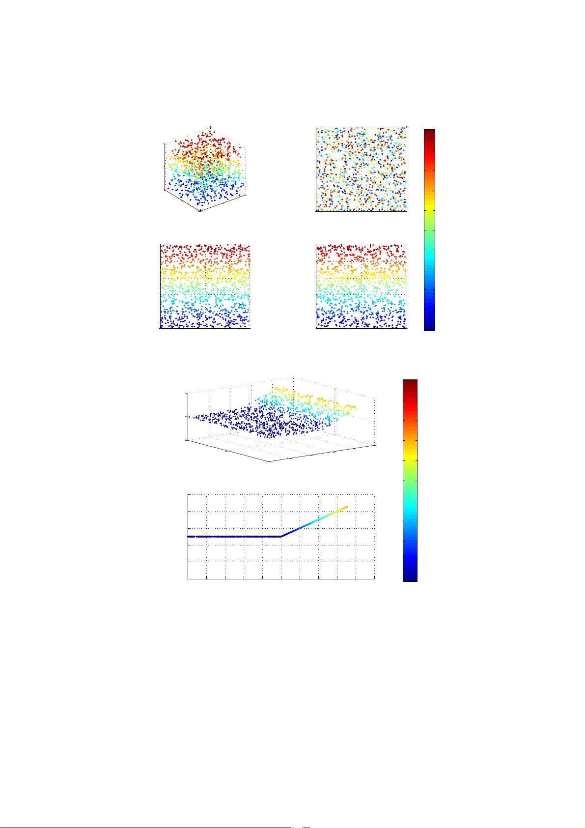
A DISCRETE AD APTED HIERARCHICAL B ASIS SOL VER FOR RADIAL B ASIS FUNCTION INTERPOLA TION JULIO E. CASTRILL ´ ON-CAND ´ AS, JUN LI, AND VICTOR EIJKHOUT A B S T R AC T . In this paper we de vel op a discret e Hierarchical Basis (HB) to ef ficient ly solve the Ra- dial Basis Funct ion (RBF) interpol ation proble m with vari able polynomial degree . The HB forms an orthogona l set and is adapted to the kern el see d fu nction and the pl acement of the inte rpolati on nodes. Moreov er , this basis is orthogona l to a set of polynomia ls up to a giv en degre e de fined on the inter- polati ng node s . W e are thus able to decouple the RBF inte rpolati on problem for any degree of the polynomia l interpolatio n and solve it in t wo steps: (1) The polynomia l orthogonal RBF interpol ation problem is effici ently solved i n the transformed HB basis with a GMRES i terati on and a d iagonal (or block SSOR) preconditi oner . (2) The residual is t hen projecte d onto an orthonormal polynomial basis. W e app ly our approach on seve ral test cases to study its eff ecti veness. 1. I N T R O D U C T I O N The computational cost f or extractin g RBF represen tations can be prohibitively expensive fo r ev en a moderate amou nt o f in terpolation nodes. For an N -po int in terpolation p roblem using direct methods it requir es O ( N 2 ) memory and O ( N 3 ) comp utational cost. Moreover , since many of the most accur ate RBFs have glob ally sup ported and increasing kernels, this pr oblem is often badly condition ed and difficult to solve with iterative methods. In th is paper we develop a fast, stable a nd memory ef ficient algor ithm to solve the RBF inter polation problem based on the construction o f a discrete HB. Dev elopmen t of RBF interp olation algorithm s has been widely studied in scientific compu ting. In general, current fast solvers are not yet optimal. On e cruc ial observation of the RBF interpolation problem is that it can be po s ed a s a discrete form of an integral equ ation. This insight allows us to extend the techn iques originally introdu ced for integral e quations to the ef ficie nt so lution of RBF interpolatio n problems. RBF in terpolation has been studied for several decad es. In 1977 Duch on [23] introduced one of the most we ll known RBFs, the thin-plate spline . This RBF is popu lar in practice since it leads to minimal energy interpolan t between the interpola tion nod es in 2D. In [2 4 ] Franke studied the approx imation capabilities of a large class of RBFs and concluded that the biharm onic spline and the multiquad ric gi ve the b est ap proximation. Furthermo re, error estimates for RBF interpolation have been dev eloped by Schaback et al. [5 2 , 4 6 , 47] and more recently by Narcowich et al. [36]. RBFs are of m uch inter est in the area of visua lization and a nimation. They have fou nd applica- tions to point clou d recon structions, denoising and repairing of meshes [13]. I n g eneral, they have been used for the reco nstruction of 3 -D objects and defor mation of these o bjects [38]. For these ar- eas of app lications it is usu ally sufficient to consider zero and linea r -degree polynom ials in the RBF problem s. Howe ver, other ap plications, such as Neural Networks and classification [55], bou ndary and finite element method s [21, 22], require consideration of higher-degree polynom ials. More recently , the c onnection between RBF interpolation, Gen er alized Least Squar es (GLSQ) [45] an d its extension to the Best Un biased Linear Estimator (BLUE) p roblem has b een established 2010 Mathe matics Subject Classification . 65D05 , 65D07, 65F25, 65F10, 62J05, 41A15. K e y words and phrases. Radial Basis Funct ion and Interpolati on and Hierar chical Basis and Inte gral equati ons and Fast Summation Methods and Stable Comple tion and Lift ing and Generalize d Least Squa res and Best Linear Unbiased Estimator . 1 2 JULIO E. CASTRILL ´ ON-CAND ´ AS, JUN LI, AND VICT OR EIJKHOUT [37, 3 1 , 32]. If the covariance matrix of a GLSQ ( and BLUE) pr oblem is describe d by a symm etric kernel matrix of an RBF problem a mong o ther con ditions, the two pr oblems beco me equiv a lent. Although GLSQ is of high interest to the statistics community , as shown b y th e high nu mber of citations of [45], the lack of fast solvers lim its its ap plication to small to medium size problem s [31, 32]. Moreover , many of these statistical problem s in volve higher than zero- and linea r -degree polyno mial regression [54, 53, 43, 33, 34, 5 0 ]. By exploiting the connec ti on between GLSQ an d RBFs, we will be able to solve GLSQ using the fast solvers d e veloped in th e RBF and in te g ral equation commu nities. For the BLUE Krig ing estimator there is less need o f higher order po lynomials. In many cases quadra ti c is sufficient for high accuracy estimation. The q uadratic interpolant leads to much better estimate than constant o r line ar . In addition , in [29] the author uses s econd de gree polynom ial BLUE for repairing surfaces. Recently Gumerov et al. [27] de veloped a RBF solver with a Krylov subspace method in c on- junction with a precon ditioner constructed fro m Cardina l function s. W e note that this approach , to our k no wled ge, is the state of the art for zero- de gree interpolation in R 3 with a biharmo nic spline. This makes it very usefu l for interpolation prob lems in co mputer grap hics. On the other hand, its application to regression problems s uch as GLSQ is limited. A domain decomp osition method was d e veloped in [8] by Beatson et al. This metho d is a mod- ification of the V on Neumann’ s altern ating algorithm, wh ere the glob al solution is appr oximated by iterating a series of local RBF interp olation p roblems. This method is promising and has led to (cou- pled with multi-po le expansions) O ( N log ( N )) computation al cost for certain in terpolation pro blems. Although th e metho d is very ef ficien t and exhibits O ( N log ( N )) computational complexity , this seems to be true for small to medium size prob lems (up to 5 0,000 no des in R 3 ) with smoo th d ata. Beyond that rang e the computatio nal cost incr eases quadratically as shown in [8]. Other results for non smooth data shows that the comp utational complexity is more err atic [14]. Furthe rmore, in many cases, it is not obvious ho w to pick the optimal domain decomposition scheme. An alter nati ve approach was developed by Beatson e t al. [7], which is based on prec onditioning and cou pled with GMRES iteration s [44]. This app roach relies on the co nstruction of a po lynomial orthog onal basis, similar to the HB approac h in our paper . T his ap proach g i ves rise to a highly sparse representatio n of the RBF interpo lation ma trix that can be very easily precond itioned by means of a diag onal matrix. The new system of equa tions exhibits condition n umber growth of no more than O ( log N ) . The downside is that this basis is not com plete. This is ameliorated by the introduction of non decaying elements, but no gu arantees on accur ac y can be made. Our appro ach is based on posing th e RB F interpolation prob lem as a discretization of an integral equation and applying p reconditioning techniqu es. This appr oach has many parallels with the work developed by Beatson et al. [7]. Howe ver , ou r approach was developed from work don e f or fast integral equation solvers. Most o f th e work in the area of fast integral equation solvers has be en r estricted to the efficient computatio n of matrix vector produ cts as part of an iterative scheme. For th e Poisson kernel the much celebrated multi- pole spherical harmon ic expansions leads to a fast sum mation algorithm that red uces each matrix-vecto r multiplication to O ( N ) compu tational steps [ 26 , 6]. This techniq ue has b een extended to a class of polyharm onic splines and multiqua drics [5, 19]. More recently L. Y ing et al. has developed multipole algorithms for a general class of kernels [56]. In contrast, the dev elopmen t of optimal (or good) precond iti oners for integral equations has been more limited. A unified appro ach for solving integral eq uations efficiently was in troduced in [1, 2, 9]. A wa velet basis was used for sparsifying the discretized operator and only O ( N log 2 2 ( N )) entr ies of the dis- cretization matrix are needed to achieve optimal asymp totic convergence. The downside is that it was limited to 1D problems. In [17] a class of m ultiw av elets based on a generalization of Hierar chical Basis ( HB) fun ctions was intro duced for sp arsifying integral equa tions on conform al surface meshes in R 3 . These wa velets A DISCRET E ADAPTED HIERARCHICAL BASIS SOL VER FOR RADIAL BASIS FUNCTION INT ERPOLA TION 3 are continu ous, multi-dime nsional, multi-resolutio n and spatially adaptive. These con structions are based on the work on Lifting by Schro der an d Swe ldens [48] an d lead to a class of adap ted HB o f arbitrary polynom ial degree . A similar ap proach was also developed in [51]. These construction s provid e co mpression cap abilities that are independ ent of the ge ometry and require only O ( N log 3 . 5 4 ( N )) entr ies to achieve optimal asymptotic con vergence . This is also true for complex geome trical f eatures with sharp edges. Moreover , this basis has a multi-resolu tion structu re that is related to the BPX schem e [39], ma king them a n excellent basis to pr econdition integral and partial differential equations. In [20] Heed ene et al. demonstrate how to use this b asis to b u ild scale decoup led stiffness matrices f or partial differential equatio ns (PDEs) over n on unif orm irregular confor mal m eshes. In this paper, we develop a discre te HB f or solving isotro pic RB F interpolation pro blems ef fi- ciently . Our HB construction is ada pted to the topology o f the interpolating nodes a nd the kernel. This new basis decoup les the p olynomial in terpolation from the RBF part, leading to a system of equations that are easier to solve. W ith o ur sparse SSOR [25, 30] or d iagonal precon ditioner , com- bined with a fast summation method, the RB F interp olation prob lem can be solved ef ficiently . Our contributions inclu de a method with asymptotic complexity costs similar to Gumerov et al [27] for problems in R 3 . However , th eir app roach is restricted to o nly constant degree RB F inter- polation. Due to th e d ecoupling of the po lynomial inter polation, o ur app roach is mo re flexible and works well for higher degree polyno mials. W e show similar results for the multiquad ric RBFs in R 3 . In con trast we did no t ob serve multiqua dric results f or R 3 in [27] and to our knowledge this result is not av ailable . Note that th e idea of de coupling the RBF sy s tem o f equations from th e polynom ial interpolatio n h as also been prop osed in [49] and [8]. In the rest of Sectio n 1 w e explicitly pose the RBF interp olation problem. In Section 2, we construct an HB th at is adapted to the interpolating nod es and the kerne l seed fun ction. In Section 3 we demo nstrate how the adapted HB is used to for m a multi-resolution RBF matrix , which is used to solve the interpolation pro blem efficiently . In section 4, we sho w some n umerical r esults of ou r method. Th e interp olating n odes are rando mly p laced, moreover the interpolating values themselves contain random noise. W e summarize our conclusion s in section 5. During the writing o f th is paper we b ecame aware of the H-Matrix appr oach by Hackbusch [10] applied to stoch asti c ca pacitance extraction [5 7 ] pr oblem. In [11] the authors apply an H- matrix appro ach to sparsify the kernel matrix arising from a Gaussian process regression problem to O ( N log N ) . In our paper, we apply HB to precon dition the RBF system, althou gh we could also use them to sparsify it. Instead , we u s e a fast summation ap proach to comp ute the matrix-vector produ cts. 1.1. Radial Basis Function Interpolation. In this section we pose the pro blem of RBF interpo la- tion for bounde d f unctions defined on R 3 . Alth ough our exposition is only for R 3 , the RBF problem and our HB approac h ca n be extended to any finite dimension. Consider a function f ( ~ x ) : R 3 → R in L ∞ ( R 3 ) and its evaluation o n a set of u ser -specified sam - pling of distinct nodes X : = { ~ x 1 , ...,~ x N } ⊂ R 3 , whe re ~ x = [ x 1 , x 2 , x 3 ] H , unisolvent with re s pect to all polyno mials o f degree at mo s t m . W e are interested in constructing approximation s to f ( ~ x ) of the form s ( ~ x ) = M ( m ) ∑ i = 1 c [ i ] q i ( ~ x ) + N ∑ j = 1 u [ j ] K ( ~ x ,~ x j ) , where K : R 3 × R 3 → R , u ∈ R N , c ∈ R M ( m ) and P : = { q 1 ( ~ x ) , . . . , q M ( m ) ( ~ x ) } is a basis f or P m ( R 3 ) , i.e. the set of all polyn omials of total degree at most m in R 3 (Note th at M ( m ) is the number of polyno mials that fo rm a ba s is for P m ( R 3 ) i.e. M ( m ) =  m + 3 3  ). This in terpolant must satisfy the following cond ition s ( ~ x j ) = f ( ~ x j ) , j = 1 , . . . , N , 4 JULIO E. CASTRILL ´ ON-CAND ´ AS, JUN LI, AND VICT OR EIJKHOUT for all ~ x j in X . Moreover , to en s ure the interpolation is unique we add the following constraint (1) N ∑ j = 1 u [ j ] q ( ~ x j ) = 0 , for all p olynomials q ( ~ x ) of degree at most m . Now , since M ( m ) is the m inimum amoun t of nodes needed to solve the poly nomial p roblem, we need at least N > M ( m ) RBF centers. The interp olation problem can be re written in matrix forma t as  K Q Q H O   u c  =  d 0  , (2) where K i , j = K ( ~ x i ,~ x j ) with i = 1 . . . N and j = 1 . . . N ; d ∈ R N such th at d j = f ( ~ x j ) ; c ∈ R M ( m ) ; and Q i , j = q j ( ~ x i ) with i = 1 . . . N , j = 1 . . . M ( m ) . Deno te the co lumns of Q as [ q 1 , . . . , q M ( m ) ] . Th is is the gen eral f orm o f th e RBF inter polation isotro pic p roblem. The p roperties of this approximation mostly depen d on the seed function K ( ~ x ,~ y ) . An example of a well known isotropic kernel in R 3 is the biharmon ic sp li ne (3) K ( ~ x ,~ x j ) : = K ( | ~ x − ~ x j | ) =   ~ x − ~ x j   . This is a p opular kernel du e to the optimal smoothness of the interpolant [8]. Th is kernel has been successfully applied in point cloud r econstructions, den oising and re pairing of meshes [13]. Mo re recently , there has been interest in extensions to anisotro pic kernels [15, 16], i.e. K ( ~ x ,~ x j ) : = K    T j ( ~ x − ~ x j )    , where T j is a 3 × 3 matrix. Th e stabilization method introduce d in this paper can be extended to solv- ing ef ficiently the RBF problem with s patially v ary ing kernels. By using the sp arsification properties of the adap ted HB a sparse represen tation of the spatially varying RBF matrix can be co nstructed in optimal time. Howev er , in this paper we restrict th e analysis to isotropic kernels in R 3 , i.e. T j = α I where α > 0. One aspect of RBF inter polation is the invertibility o f th e matrix in E quation (2). I n [35] it is shown that the interpolation problem (2) has a un ique solution if we assume th at the interpo lating nodes in X a re unisolvent with respect to P m ( R 3 ) and the continu ous kernel is s trictly condition ally positive (or ne g ative) definite . Before we gi ve t he definition, we provide some notation. Definition 1 . Suppose that X ⊂ R 3 is a set of interpola ting nodes and { q 1 ( ~ x ) , q 2 ( ~ x ) , . . . , q M ( m ) ( ~ x ) } is a basis for P m ( R 3 ) , then we use P m ( X ) to deno te the column space of Q. W e now assume the kernel matrix K satisfies the following ass umption . Definition 2. W e say that the symmetric function K ( · , · ) : R N × R N → R is strictly con ditionally positive definite of de g r ee l if for all sets X ⊂ R 3 of distinct nodes v H K v = N ∑ i , j = 1 v i v j K ( ~ x i ,~ x j ) > 0 , for all v ∈ R N such th at v ⊥ P l ( X ) an d v 6 = 0 . Alternatively , und er the same assumptions, K ( · , · ) : R N × R N → R is strictly con ditionally negative defin ite if v H K v < 0 , for all v ∈ R N such that v ⊥ P l ( X ) . The in vertibility of the RBF interpolation problem can be proven by the basis construction de vel- oped in th is paper . Althou gh this is not necessary , it does cast insights on how to c onstruct a basis that can solve the RB F Prob lem (2) efficiently . A DISCRET E ADAPTED HIERARCHICAL BASIS SOL VER FOR RADIAL BASIS FUNCTION INT ERPOLA TION 5 1.2. Decoupling of t he RBF interp olation problem. Supp ose there exists a matrix T : R N − M → R N , where M : = d im ( P m ( X )) , such that T H annihilates any vector v ∈ P m ( X ) (i.e. T H v = 0 ∀ v ∈ P m ( X ) ). Furtherm ore, suppo se there exists a second m atrix L : R M → R N such that the com bined matrix P : = [ L T ] is o rthonormal such that P H : R N → R N maps R N onto P m ( X ) ⊕ W , where W : = ( P m ( X )) ⊥ . Su ppose that u ∈ P m ( X ) ⊥ , then u = T w for some w ∈ R N − M . Problem (2 ) can now be re-written as T H K T w + T H Qc = T H d . Howe ver, since the columns of Q belong in P m ( X ) then (4) T H K T w = T H d . From Definition 2 an d the orthono rmality of P we conc lude that w can b e solved un iquely . Th e second step is to solve the equation L H Qc = L H d − L H K T w . From the u nisolvent prop erty of the nodes X the m atrix Q h as rank d im ( P m ( R 3 )) , m oreover , L also has ran k d im ( P m ( R 3 )) , th us L H Q has full rank and it is in vertible. Although proving the existence of P and hen ce the uniquen ess o f the RBF prob lem is an in terest- ing exercise, there are mo re practical implications to the constructio n of P . First, the coupling of Q and K can lead to a system of ill-con ditioned equations dependin g on the scale o f the domain [ 8 ]. The decouplin g property of the transform P leads to a scale indepe ndent problem , thus corre cting this source of ill-co nditioning. But mo re impo rtantly , we fo cus on the structure of T H K T a nd how to exploit it to solve the RBF interpo lation pro blem (2) efficiently . The key idea is the ability of T H to vanish discrete polynomial moments and its effect on the matrix K ( · , · ) . W e shall now restrict ou r attention to Kernels that satisfy the following assumption. Assumption 1. Let D α x : = ∂ α 1 , α 2 , α 3 ∂ ~ x α 1 1 ∂ ~ x α 2 2 ∂ ~ x α 3 3 and similarly for D β y , we assume that D α x D β y K ( ~ x ,~ y ) 6 C | ~ x − ~ y | q + | α | + | β | , wher e α = ( α 1 , α 2 , α 3 ) ∈ Z 3 , | α | = α 1 + α 2 + α 3 , and q ∈ Z . I n a ddition, we assume that K ( ~ x , · ) and K ( · ,~ y ) ar e ana lytic everywher e except for ~ x = ~ y. This assumptio n is satisfied by many practical kern els, such as multiqu adrics and p olyharmonic splines [24, 8]. 2. A D A P T E D D I S C R E T E H I E R A R C H IC A L B A S I S C O N S T RU C T I O N S In this section we show how to construct a class of discrete HB that is ada pted to th e kernel function K ( · , · ) and to the local interpo lating nodes (or interp olating nodes) contained in X . The objective is to solve RBF interpolation Pro blem (2) efficiently . The HB method will be divided into the following parts: • Multi-resolution domain dec omposition. The first part is in essence a prep rocessing step to build cubes at dif f erent levels of resolution as place holde rs for the interpo lation nodes belongin g to X . • Adapted discrete HB construction. From the m ulti-resolution do main decompo sition of the interp olating nodes in X , an adapted multi-resolution b as is is constructed that annihilates any polynom ial in P p ( X ) , where p ∈ Z + and p > m . p will b e in essence the degree of the Hierarchical Basis, which is not to be confu sed with m . • GMRES iterations with fast s ummation method. Wi th the adap ted HB a multi-resolution RBF interpo lation matrix is implicitly obtained th rough a f a s t summation method and solved iterativ ely with a GMRES algorithm and an SSOR or diagonal precond itioner . 6 JULIO E. CASTRILL ´ ON-CAND ´ AS, JUN LI, AND VICT OR EIJKHOUT 2.1. Multi-resolution Domain Decomposition. W ithout loss of generality , it is assum ed that th e interpolatin g nodes in X are c ontained in a cube B 0 0 : = [ 0 , 1 ] 3 . The next step is to form a series of le vel depend ent c ubes that serve as place holders for the interpolating nodes at each le vel of resolutio n. The basic algo rithm is to subd i vide the cu be B 0 0 into eight cu bes if | B 0 0 | > M ( p ) , wher e | B j k | denotes the to tal nu mber of interpolating nodes conta ined in the cube B k j . Subseque ntly , each cub e B j k is sub -di v ided if | B j k | > M ( p ) until there are at most M ( p ) interpo lating nodes at the finest lev e l. The algorithm is explained more in detail in the follo w ing pseudo -code: Input : X : = { ~ x 1 ,~ x 2 , . . . ,~ x N } , M ( p ) Output : B j k ∀ k ∈ { K ( 0 ) , . . . , K ( n ) } , n begin pre-pr ocessing; j ← 0 ; B 0 0 ← [ 0 , 1 ] 3 ; K ( 0 ) ← { 0 } ; main; while | B j k | > M ( p ) for any k ∈ K ( j ) do K ( j + 1 ) ← / 0 ; for k ← 0 to | K ( j ) | do forming B j + 1 8 k , . . . , B j + 1 8 k + 7 ; K ( j + 1 ) ← K ( j + 1 ) ∪ 7 w = 0 8 k + w ; end j ← j + 1 ; end n ← j end Algorithm 1: Multi-resolu tion Domain Decomposition Remark 1. K ( j ) is an in de x set fo r all the cubes at level j . W e u s e | K ( j ) | to denote the car din ality of K ( j ) . Remark 2. Fi nding the distance between any two boxes can be p erformed in O ( N ( n + 1 )) compu ta- tional steps by applying an octree algorithm. Ther efor e the Multi-r esolution Domain Decomposition algorithm can be pe r formed in O ( N ( n + 1 )) co mputational steps. Th is can be easily seen since the maximum number of boxes at any level j is bou nded by N and ther e is a total of n + 1 levels. Before describing the construction of the adapted discrete HB, we introduce some more notations to facilitate our discussion. Definition 3. Let B j be the set of all th e cubes B j k at level j that co ntain at least one in terpolating center fr om X . Definition 4. Let C : = { e 1 , . . . , e N } , wher e e i [ i ] = 1 and e i [ j ] = 0 if i 6 = j . Furthermor e, define the bijective mappin g F p : C → X such that F p ( e i ) = ~ x i , for i = 1 . . . N and F q : C → Z + s.t. F q ( e i ) = i. Now , for eac h cube B n k ∈ B n at the finest level n, let B n k : = { e i | F p ( e i ) ∈ B n k } . and for all l = 1 , . . . , n − 1 ˜ B l k : = { e i | F p ( e i ) ∈ B l k } . Definition 5. Let C n : = S k ∈ K ( n ) B n k . Definition 6. F or all j = 0 , . . . , n − 1 , let chil d r en ( B j k ) be the collection of nonemp ty subdivided cubes B j + 1 l ∈ B j + 1 , for some l ∈ N , of the cube B j k . Definition 7. F or every n on emp ty B j k let the set parent ( B j k ) : = { B j − 1 l ∈ B j − 1 | B j k ∈ chil d r en ( B j − 1 l ) } . A DISCRET E ADAPTED HIERARCHICAL BASIS SOL VER FOR RADIAL BASIS FUNCTION INT ERPOLA TION 7 2.2. Basis Construction. From the output of the multi-resolutio n d ecomposition Algo rithm 1 we can now build an adapted discrete HB that annihilates any po lynomial in P p ( X ) . T o construct such a basis, we apply the stable comple ti on [ 12] pro cedure. This approach was followed in [17]. Howe ver, the basis is furth er o rthogonalized by using a modified Singu lar V alu e Decom position (SVD) orthon ormalization ap proach introd uced in [51]. Suppose v 1 , . . . , v s are a set of orthono rmal vector s in R N , where s ∈ Z + , a new basis is co nstructed such that φ j : = s ∑ i = 1 c i , j v i , j = 1 , . . . , a ; ψ j : = s ∑ i = 1 d i , j v i , j = a + 1 , . . . , s , where c i , j , d i , j ∈ R and fo r som e a ∈ Z + . W e desire th at the new discrete HB vector ψ j to be orthog onal to P p ( X ) , i.e. (5) N ∑ k = 1 r [ k ] ψ j [ k ] = 0 , for all r ∈ P p ( X ) . Notice that the summ ation and the vector s r and ψ j are in the same or der as the entries of the set X. Due to the ortho normality of the basis { v i } s i = 1 this implies th at Eq uation (5) is satisfied if the vector [ d i , 1 , . . . , d i , s ] belong s to the null space of the matrix M s , p : = Q H V , where the columns of Q a re a basis fo r P p ( X ) ( i.e. all the polyn omial mome nts) and V = [ v 1 , v 2 , . . . , v s ] . (Notice that the order of th e sum mation is d one with respect to the set X) . Sup pose that the matrix M s , p is a rank a matrix and let U s , p D s , p V s , p be the SVD decompo sition. W e then pick (6)      c 0 , 1 . . . c a , 1 d a + 1 , 1 . . . d s , 1 c 0 , 2 . . . c a , 2 d a + 1 , 2 . . . d s , 2 . . . . . . . . . . . . . . . . . . c 0 , s . . . c a , s d a + 1 , s . . . d s , s      : = V H s , p , where the colu mns a + 1, . . . , s f orm an orthonorma l basis of the nullspace N ( M s , p ) . Similarly , the columns 1 , . . . , a f orm an ortho normal basis of R N \ N ( M s , p ) . Remark 3. If { v 1 , . . . , v s } is orthonorma l, then new ba sis { φ 1 , . . . , φ a , ψ a + 1 , . . . , ψ s } is orthonorma l, and spans the same space as s pa n { v 1 , . . . , v s } . This is due to the orthonormality of the matrix V s , p . Remark 4. If s is la r ger than the total n umber o f va nishing momen ts, th en M s , p is guaranteed to have a nullspa ce of at least rank s − M ( p ) , i.e. there exist at least s − M ( p ) o rt hono r mal vectors { ψ i } that satisfy Equation 5. 2.3. Finest Level. W e can now build an o rthonormal mu lti-resolution ba s is. First, choose a priori the degree of moments p and start at the finest lev el n . The n e x t step is to pr ogressi vely build th e adapted HB as the le vels are tra versed. At the finest le vel n , for each cube B n k ∈ C n let v i : = e i for all e i ∈ B n k . As described in the previous section, the objective is to build ne w func tions φ n k , l : = s ∑ i = 1 c n , i , l , k v i , l = 1 , . . . , a n , k , ψ n k , l : = s ∑ i = 1 d n , i , l , k v i , l = a n , k + 1 , . . . , s , such that Equation (5) is satisfied. The first step is to form the matrix M n , k s , p : = Q H V , whe re the colum ns of Q are a basis for P p ( X ) . Notice th at since e i [ w ] = 0 for w 6 = i and e i ∈ B n k , then o nly | B n k | columns of Q H are n eeded to fo rm the matrix M n , k s , p and the rest can be thrown a way since th e y multiply with zero. 8 JULIO E. CASTRILL ´ ON-CAND ´ AS, JUN LI, AND VICT OR EIJKHOUT The n e x t step is to ap ply the SVD pr ocedure such th at M n , k s , p → U n , k s , p D n , k s , p V n , k s , p . T he coefficients c n , i , j , k and d n , i , j , k are then obtained from the rows of V n , k s , p and a n , k : = rankM s , p . Now , for each B n k ∈ B n denote ¯ C n k as the collectio n of basis vectors { φ n k , 1 , . . . , φ n k , a n , k } , and similarly denote ¯ D n k as the collection of basis vectors { ψ n k , a n , k + 1 , . . . , ψ n k , s } . Furtherm ore, we define the detail subspace W n k : = s pan { ψ n k , a n , k + 1 , . . . , ψ n k , s } and the average subspace V n k : = s pan { φ n k , 1 , . . . , φ n k , a n , k } . By collecting the transform ed vecto rs from all the cubes in C n , we form the subspaces V n : = ⊕ k ∈ K ( n ) V n , k , W n : = ⊕ k ∈ K ( n ) W n , k , where ⊕ is a direct sum and K ( i ) : = { k | B i k ∈ B i } . Remark 5. W e first observe th at R N = V n ⊕ W n ⊕ ˜ V n , wher e ˜ V n is the spa n of all the u nit vecto r s contained in {{ ˜ B l k } k ∈ K ( l ) } n − 1 l = 1 . This is true sin ce the number of interp olating nodes is equal to N and R N = s pan { e 1 , e 2 , . . . , e N } . Remark 6. It is possible that W n k = / 0 for some p articular cu be B n k . This will be the case if the car d inality of B n k is less or equa l to M ( p ) i.e. th e dimension of the nu lls pace of M s , p is zer o. However , this w ill not be a pr oblem. As we s hall see in section 2.4, the ne xt set of HB are built fr om the vectors in ¯ C n k and its siblings. Lemma 1. The basis vectors of V n and W n form an orthonormal set. Pr oof. First no ti ce th at since B n l ∩ B n k = / 0 whenever k 6 = l then V n , k ⊥ V n , l , W n , k ⊥ W n , l and V n , k ⊥ W n , l . The result follows from the fact that the rows V n , k s , p form an orthono rmal set.  It is clear that the detail subspace W n ⊥ P p ( ~ x ) , but the average sub space V n is not. Howe ver, we can still perform th e SVD procedur e to fu rther d ecompose V n . T o this en d we need to accu mulate the avera ge b asis vectors of V n and all the unit basis vectors in { ˜ B n − 1 k ∈ K ( n − 1 ) } . For each B n − 1 k ∈ B n − 1 identify the set chil d ren ( B n − 1 k ) . Form the set B n − 1 k : = { ¯ C n l | B n l ∈ chil d ren ( B n − 1 k ) } . If B n 1 k has no children then B n − 1 k = ˜ B n − 1 k . W e can now apply the SVD procedur e o n each s et of average vectors in B n − 1 k . 2.4. Intermediate Level. Suppose we hav e the collection of sets B i k for all k ∈ K ( i ) . For each B i k perfor m the matrix decomp osition M i , k s , p = U i , k s , p D i , k s , p V i , k s , p for all v ∈ B i k . Fro m the matrix V i , k s , p obtain the decomp osition φ i k , l : = s ∑ j = 1 c i , j , l , k v j , l = 1 , . . . , a i , k , ψ i k , l : = s ∑ j = 1 d i , j , l , k v j , l = a i , k + 1 , . . . , s , where the coefficients c i , j , l , k and d i , j , l , k are obtained from the rows of V i , k s , p in (6) and a i , k : = rank M i , k s , p . Then we form the subspaces W i k : = s pan { ψ i k , a i , k + 1 , . . . , ψ i k , s } , V i k : = s pan { φ i k , 1 , . . . , φ i k , a i , k } , and V i : = ⊕ k ∈ K ( i ) V i , k , W i : = ⊕ k ∈ K ( i ) W i , k . It is e as y to see th at V i + 1 = V i ⊕ W i ⊕ ˜ V i , , where ˜ V i is the span of a ll the unit vectors contain ed in {{ ˜ B l k } k ∈ K ( l ) } i l = 1 . The basis vectors are collected into two grou ps: Definition 8. F or each B i k ∈ B i that ha ve children let the sets, for i = 0 , . . . , n − 1 , ¯ C i k : = { φ i k , 1 , . . . , φ i k , a i , k } , and ¯ D i k : = { ψ i k , a n , k + 1 , . . . , ψ i k , s } . A DISCRET E ADAPTED HIERARCHICAL BASIS SOL VER FOR RADIAL BASIS FUNCTION INT ERPOLA TION 9 Just as for the fin est lev el case, we can f urther decomp ose V i . T o this end, for each B i − 1 k ∈ B i − 1 identify the set chil d ren ( B i − 1 k ) and form the set B i − 1 k : = { ¯ C i l | B i l ∈ chil d ren ( B i − 1 k ) } . If B i − 1 k has no children then B i − 1 k = ˜ B i − 1 k . 2.5. Coarse Lev el. It is clear that when the iteration reaches V 0 the basis function no longer a nni- hilates po lynomials of degree p . Howev er , a new basis can be o btained that can vanish polyn omials of degree m . Recall that for the RBF interp olation p roblem with polynomial degree m it is imposed that u ⊥ P m ( X ) . If p = m then it is clear that u ∈ W 0 ⊕ . . . W n and RBF problem deco uples as shown in Section 1. Ho wever , if p > m then u ∈ ( P p ( X ) \ P m ( X )) ⊕ W 0 ⊕ . . . W n and the RBF prob lem does not decouple. It is then of interest to find an orthon ormal basis to P p ( X ) \ P m ( X ) . This can be easily achieved. Let the co lumns of the m atrix Q be a basis f or P p ( X ) , where each function q i ( x ) correspo nds to the i t h moment. Now , the first M ( m ) co lumns cor respond to a basis for P m ( X ) . Thus an orthonorm al basis for P p ( X ) \ P m ( X ) is easily achieved b y applying t he Gram-Schmidt pro cess. Alternatively the matrix M 0 , m can no w be formed by app lying the SVD d ecomposition and a basis that annihilates all polyn omial of degree m or lower is obtained. The matrix ¯ C 0 0 can now be rep laced with the matr ix [ C − 1 0 , D − 1 0 ] , where the columns of C − 1 0 form an o rthonormal basis for P m ( X ) and D − 1 0 is an orthono rmal basis for P p ( X ) \ P m ( X ) . The complete algo rithm to decompo s e R N into a m ulti-resolution basis w it h respect to the inter- polating nodes X is d escribed in Algorith ms 2 and 3. Input : Finest level n ; De g ree of RB F m ; B j k ∀ k ∈ K ( j ) , j = − 1 . . . n ; B n k ∀ k ∈ K ( n ) ; {{ ˜ B l k } k ∈ K ( l ) } n l = 1 ; Degree of v an ishing moments p > m ; X . Output : { ¯ C − 1 0 , ¯ D − 1 0 , ¯ D 0 0 , ¯ D 0 1 , . . . , ¯ D n k } main; for j ← n to 1 step − 1 do for k ← 1 t o | K ( j − 1 ) | do B j − 1 k ← / 0 end for k ← 1 t o | K ( j ) | do { ¯ D j k , ¯ C j k } ← PolyOrtho ( B j k , p ); U ← paren t ( B j k ) ; forall the B j − 1 l ∈ U do B j − 1 l ← B j − 1 l ∪ ¯ C j k ; end forall ˜ B j − 1 k ∈ B j − 1 let B j − 1 k = ˜ B j − 1 k ; end end { ¯ D − 1 0 , ¯ C − 1 0 } ← PolyOrtho ( B 0 0 , m ); Algorithm 2: Adapted Discrete HB Construction Lemma 2. R N = V 0 ⊕ W 0 ⊕ . . . W n = s pan { ¯ C − 1 0 , ¯ D − 1 0 , ¯ D 0 0 , ¯ D 0 1 , . . . , ¯ D n k } . for j = 0 . . . n and for all k ∈ K ( j ) Pr oof. The result f ollo ws fr om Remark 5 an d that V i is deco mposed into V i − 1 ⊕ W i − 1 ⊕ ˜ V i − 1 for all i = 1 . . . n .  Remark 7. Whe n A lgorithm 2 terminates at level i = 0 , ther e wil l be M ( p ) orthonormal vector s t hat span P p ( X ) . 10 JULIO E. CASTRILL ´ ON-CAND ´ AS, JUN LI, AND VICT OR EIJKHOUT Remark 8. At the finest level n, the number o f vecto r s in each matrix ¯ C n k corr espo nding to B n k is bound ed by M ( p ) . Now , for each B n − 1 k ther e ar e at most 8 M ( p ) vectors fr om the children of B n − 1 k . F r om the pr oced ur e for the basis construction in section 2.2 for each B n − 1 k ther e ar e a t at most M ( p ) vectors in ¯ C n k . Furth er mor e, th er e are no mo r e than 8 M ( p ) vec tor s in ¯ D n k formed. The sa me conclusion follows for each B i k , for all levels i = 0 , . . . , n . Input : B j k , Degree of v anishin g momen t p Output : ¯ D j k , ¯ C j k ¯ C j k ← / 0; , ¯ D j k ← / 0 s ← | B j k | ; V ← [ v 1 , . . . , v s ] ; M j , k s , p ← Q H V ; [ U j , k s , p , D j , k s , p , V j , k s , p ] ← SV D ( M j , k s , p ) ; a j , k ← rank of D j , k s , p ; for l ← 1 to a j , k do φ j k , l ← ∑ s i = 1 c j , i , l , k v i ; ¯ C j k ← [ ¯ C j k , φ j k , l ] ; end for l ← a j , k + 1 to s do ψ j k , l ← ∑ s i = 1 d j , i , l , k v i ; ¯ D j k ← [ ¯ D j k , ψ j k , l ] ; end Algorithm 3: PolyOrtho( B j k , p ) Definition 9. F or any B i k , k ∈ K ( i ) , i = 0, . . . n, let | B i k | be the number of vectors in B i k . Theorem 1. The comple xity cost for Algorithm 2 is bounded by O ( N n ) . Pr oof. Suppose we start a t the fine s t level n . Now , fo r each bo x in B n k , the vectors e i ∈ B n k have at most one non-zero entry . This imp lies that the matrix M n , k s , p = Q H V , Q H is a M ( p ) × | B n k | matrix an d V is at most a | B n k | × | B n k | matrix. Th en t he total cost to computin g M n , k s , p for all k ∈ K ( n ) is bou nded by C ∑ k ∈ K ( n ) | B n k | 2 M ( p ) for some C > 0. Now since   ∪ k ∈ K ( n ) B n k   = N and | B n k | is at most M ( p ) ∀ k ∈ K ( n ) , then t he cost for computin g ¯ C n k and ¯ D n k , ∀ k ∈ K ( n ) , i s at most O ( N ) . At lev e l n − 1, from Remark 8 we see that ther e are at mo st 8 M ( p ) vectors in each B n − 1 k ∀ k ∈ K ( n − 1 ) . Forming the the ma trix M n − 1 , k s , p = Q H V , Q H is at most M ( p ) × | B n − 1 k | an d V is at mo st | B n − 1 k | × | B n − 1 k | . Now , since   ∪ k ∈ K ( n − 1 ) B n − 1 k   = N it follows th at th e cost for co mputing M n − 1 , k s , p , ∀ k ∈ K ( n − 1 ) , is at most O ( N ) . Furthermore, we hav e from Remark 8 that | B n − 2 k | 6 8 M ( p ) , ∀ k ∈ K ( n − 2 ) . Since for each le vel i ,   ∪ k ∈ K ( i ) B i k   6 N , then th e total cost of com puting M i , k s , p , ∀ k ∈ K ( i ) , is at most O ( N ) and | B i − 1 k | 6 8 M ( p ) , ∀ k ∈ K ( i − 1 ) . The result follows.  2.6. Properties. The adapted HB co nstruction has some interesting properties. In particular, the space R N can b e deco mposed in a series of n ested subspaces that are or thogonal to P p ( X ) a nd the basis f orms an o rthonormal set. As a side benefit, this series of nested subsp aces can b e used to prove the uniq ueness of the RBF interpolatio n pro blem. On e impor tant pro perty of the adapted HB is presented in the following lemma. Lemma 3. The basis of R N described by th e vecto r s of { ¯ C − 1 0 , ¯ D − 1 0 , ¯ D 0 0 , ¯ D 0 1 , . . . , ¯ D n k } , j = 0 . . . n, k ∈ K ( j ) form an orthonormal set. Pr oof. W e prove this by a simple indu ction argumen t. Assume that f or le vel i the set of vectors { B i k } are orth onormal. Since the r o ws of the set V i , k s , p are orthonorm al an d B i l ∩ B i k = / 0 whenever l 6 = k , then A DISCRET E ADAPTED HIERARCHICAL BASIS SOL VER FOR RADIAL BASIS FUNCTION INT ERPOLA TION 11 it follows that the vectors ∪ k ∈ K ( i ) { ¯ C i k , ¯ D i k } form an or thonormal basis. T he result then follows from Lemma 1.  Definition 10. Given a set of unisolvent in terpolating n odes X ⊂ R 3 with r espect to P p ( R 3 ) , we form the matrix P fr om the basis vectors { ¯ C − 1 0 , ¯ D − 1 0 , ¯ D 0 0 , ¯ D 0 1 , . . . , ¯ D n k } . From Lemmas 2 and 3 the matrix P has the following prope rties (1) If v ∈ P p ( X ) then P H v has d im ( ¯ C 0 0 ) non-ze ro entr ies. (2) PP H = P H P = I . 3. M U LT I - R E S O L U T I O N R B F R E P R E S E N TA T I O N The HB we constructed above is adapted to the kernel and the location of the interp olation n odes. It also satisfies the vanishing moment prop erty . The construction of such an HB leads to several importan t consequ ences. First, we can use th e basis to p rov e the existence of a unique solution of the RBF prob lem, b ut more importantly , this basis can be used to solve the RBF prob lem efficiently . As the reader might recall from section 1.1, the co nstruction of the adapted HB decouples the polyno mial in terpolant from the RBF functions if the degree of the vanishing moments p is equal to the degree of the RB F po lynomial interpo lant m . This simple result can be extended if p > m . Theorem 2. Supp ose X is unisolvent with r espect to R 3 and u solves th e interpolation p r oblem of equation (2) uniquely , wher e u ⊥ P m ( X ) an d the kernel satisfies Definition 2. If the num ber of vanishing moments p > m then  C H ⊥ KC ⊥ C H ⊥ K T T H KC ⊥ T H K T   s w  =  C H ⊥ d T H d  , (7) for some s ∈ R M − O and w ∈ R N − M , wher e T : = [ ¯ D 0 0 , ¯ D 0 1 , . . . , ¯ D n k ] , C ⊥ = ¯ D − 1 0 and O = d im ( P m ( X )) . Mor eover , u = C ⊥ s + T w. Pr oof. Since u ∈ ( P p ( X ) \ P m ( X )) ⊕ W 0 ⊕ . . . W n , then u = C ⊥ s + T w for some s ∈ R M − O and w ∈ R N − M , where O = d im ( P m ( X )) . Replacing u into (2), pre-multiplying by [ C H ⊥ T H ] H and re calling that C ⊥ , T ⊥ P m ( X ) the result follows.  Once u is fou nd, c is e as ily o btained by solvin g the set o f equations L H Qc = L H ( d − Ku ) , where L H Q ∈ R M ( p ) × M ( p ) . There are two ways we can solve this, since L an d Q spa n the sam e space and hav e full colum n rank, then L H Q is in vertible and c = ( L H Q ) − 1 L H ( d − K u ) . Alternatively , we can define the interpo lation problem in terms o f the ba s is vecto rs in L directly i.e. Q : = L , wh ich leads to c = L H ( d − K u ) . For the rest of th is section we describe the algorithms f or solving th e previous system of e quations. The entries of the matrix K W : =  C H ⊥ KC ⊥ C H ⊥ K T T H KC ⊥ T H K T  are for med fr om all the pairwise matching of any two vectors ψ i k , m , ψ j l , g from the set D : = { ¯ D − 1 0 , ¯ D 0 0 , ¯ D 0 1 , . . . , ¯ D n k } . The entries of K W take the form (8) ∑ k ∈ K ( n ) ∑ k ′ ∈ K ( n ) ∑ e a ∈ B n k ∑ e b ∈ B n k ′ K ( F p ( e a ) , F p ( e b )) ψ i k , m [ F q ( e a )] ψ j l , g [ F q ( e b )] , Notice that the summation is ov er all the vectors e o s.t. o = 1 , . . . , N . However , the entries o f ψ i k , m are mostly zeros, thus in practice the summation is over all the non-z ero terms. 12 JULIO E. CASTRILL ´ ON-CAND ´ AS, JUN LI, AND VICT OR EIJKHOUT Continuing with the same notation, the entries of d W : = T d have the form ∑ k ∈ K ( n ) ∑ e a ∈ B n k ψ i k , m [ F q ( e a )] f ( F p ( e a )) . Since w = P u and u ⊥ P p ( X ) , then entries of w have the form ∑ k ∈ K ( n ) ∑ e a ∈ B n k ψ i k , m [ F q ( e a )] u [ F q ( e a )] , ∀ ψ i k , m ∈ D . It is clear that fr om the set D the matr ix K W is o rdered such tha t the entries of any row o f K W sums over th e same vector ψ i k ∈ D . In Figure 3 a block de composition o f th e ma trix K W is sho wn . One = P S f r a g r e p l a c e m e n t s K n , n W . . . K n , 0 W . . . . . . . . . K 0 , n W . . . K 0 , 0 W w n . . . w 0 d n W . . . d 0 W F I G U R E 1 . Organiza ti on of the linear system K W w = d . Th e block matrices K i j W consist o f all th e summatio ns in Equation 8 , for all ψ i k , m , ψ j l , g ∈ D that belong to lev e l i and j . The vectors d i W correspo nd to all inner produ cts of ψ i k , m ∈ D at le vel i . Similar ly for w , wh ere w = T u . interesting observation of the matrix K W is that most of the information of the matrix is contained in a fe w entries. Indeed , for integral equation s it can be sho wn that an adapted HB discretization matrix requires only O ( N l og ( N ) 3 . 5 ) entries to achieve optimal asymptotic conv ergence [17]. Th is has been the ap proach that was followed b ehind the id ea of wa velet sparsification of in te g ral equations [ 9 , 1 , 2, 17, 3, 40, 41]. Howe ver, it is not necessary to compute th e entries of K W for efficiently in vertin g the matrix, but instead we only have to compute matr ix vector products of the submatrices K i , j W in O ( N ) or O ( N l og ( N )) com putational steps. 3.1. Preconditioner. On e key observation of the matr ix K W is that each o f th e blocks K i , j W is well condition ed. Our experiments in dicate that this is the case even for non uniform placement of the nodes. W e pro pose to use two kinds o f precond iti oners on the decoupled RBF problem: a blo ck SSOR and a diagon al preconditioner based on the m ulti-resolution matrix K W . The block SSOR multi-resolu ti on precondition er shows better iteratio n counts and is a novel approach to preco ndi- tioning. Howe ver, in p ractice, the simplicity o f th e d iagonal prec onditioner makes it easier to code and is faster per iteration count for the size of problems in which we are interested. The precondition er on the deco upled RBF takes the form of the following prob lem: (9) ¯ P − 1 K W w = ¯ P − 1 d W , A DISCRET E ADAPTED HIERARCHICAL BASIS SOL VER FOR RADIAL BASIS FUNCTION INT ERPOLA TION 13 where K W → L W + D W + L H W and L W =      0 0 0 0 K 1 , 0 W 0 0 0 . . . . . . 0 0 K n , 0 W . . . K n , n − 1 W 0      and D W =      K 0 , 0 W 0 0 0 0 K 1 , 1 W 0 0 0 0 . . . 0 0 0 0 K n , n W      . The block precond itioner is co nstructed as ¯ P = ( L W + D W ) D − 1 W ( L H W + D W ) . W e can solve this system of equatio ns with a restarted GM R ES ( or MINRES since the matrices are symmetric) iteration [44]. T o compute each iteration efficiently we need each of the matrix v ector produ cts of the blocks K i , j W to b e comp uted with a fast sum mation method . W e have the choice of either computing each block as m atrix-vector products fro m a fast summa ti on d irectly , or a spa rse precon ditioner th at can be built and stored. 3.1.1. F ast Summation. It is not n ecessary to com pute the matrix K W directly , but to em ploy ap- proxim ation methods to compute matrix-vector produ cts K W α W efficiently . T o such end we make the following ass umption . Assumption 2. Let ~ y 1 ,~ y 2 , . . . ,~ y N 1 ∈ R 3 , c 1 , c 2 , . . . c N 1 ∈ R , R BF : = s pa n ( K ( x ,~ y 1 ) , K ( x ,~ y 2 ) . . . , K ( x ,~ y N 1 )) , and T = s pa n { ˜ φ 1 , ˜ φ 2 , . . . , ˜ φ q } , for some set of linearly in dependent function s ˜ φ 1 , ˜ φ 2 , . . . , ˜ φ q . W e are inter ested in the evalua tion of the RBF map φ ( ~ x ; ~ y 1 , . . . ,~ y N 1 ) : = N 1 ∑ i = 1 c i K ( ~ x ,~ y i ) , wher e ~ x ∈ R 3 . Su ppose ther e e xists a tr ansformation F ( φ ( ~ x ; ~ y 1 , . . . ,~ y N 1 )) : R BF → T with O ( N 1 ) computatio nal and storage cost. Mor eover , a ny successive evaluation of F ( φ ( ~ x ; ~ y 1 , . . . ,~ y N 1 )) can be performed on the basis functions of T in O ( 1 ) operations and | F ( φ ( · )) − φ ( · ) | 6 C F A  1 a  ˜ p + 1 , wher e ˜ p ∈ Z + is the or der of the fast summation method, A = ∑ N 1 i = 1 | c i | , C F > 0 a nd a > 1 . There exist se veral metho ds that satisfy , or nearly satisfy , Assum ption 2. In p articular we ref er t o those based on multi-pole expansions and the Non-equidistant F ast Fourier T ransfor m [ 6 , 42, 56]. The system of equ ations (9) can now be solved using an inner and ou ter iteration proced ure. For the outer loo p a GMRES algorithm is used, whe re the search vectors are based on the matrix ¯ P − 1 K W . The inner loop consists of computin g efficiently the matrix-vector p roducts ¯ P − 1 K W α W , for some vector α W ∈ R N . Th is computation is br oken down into two steps: Step One T o comp ute efficiently K W α W for each matrix vector pro duct K i , j W α j W , we fix ψ i k , m from Equation (8) and then transform the map ∑ ψ j l , g ∈ ¯ D j ∑ ~ y b ∈ X K ( ~ x a ,~ y b ) ψ j l , g [ F q ( F − 1 p ( ~ y b ))] α j l , g , for all the vectors ψ j l , g ∈ ¯ D j , into a new basis { ˜ φ 1 , ˜ φ 2 , . . . , ˜ φ q } . Th e compu tational cost for this pro- cedure is O ( N 1 ) , where N 1 correspo nds to the number of non-zero entries of all ψ j l , g ∈ ¯ D j . Sinc e the computatio nal cost fo r ev aluatin g the n e w basis on any p oint ~ x a ∈ X is O ( 1 ) , th en the total cost for calculating each row of ¯ K i , j W α j W is O ( N 1 + N 2 ) , where N 2 is equal to all the non-zer o entries of ψ i k , m . 14 JULIO E. CASTRILL ´ ON-CAND ´ AS, JUN LI, AND VICT OR EIJKHOUT Now , since for ea ch j = 0 , . . . , n ,    ∪ k ∈ K ( j ) B j k    6 N , then N 1 is bounded b y CN for some C > 0. For the same reason N 2 is also bounded by C N . This implies that the total cost for e valuating the matrix vector products K W α W is O (( n + 1 ) 2 N ) . Step T wo : The computation of ¯ P − 1 β W , where β W : = K W α W is broken up into three stages. First, let γ W : = ( L W + D W ) − 1 β W , then       K 1 , 1 W 0 . . . 0 K 2 , 1 W K 2 , 2 W . . . . . . . . . 0 . . . 0 K n , 1 W . . . K n , n − 1 W K n , n W            γ 1 W γ 2 W . . . γ 1 W      =      β 1 W β 2 W . . . β n W      . Since ( L W + D W ) has a block trian gular from , we can solve the inv e rse-matrix vector produ ct with a bac k substitution sch eme. Suppose that we have found γ 1 W , . . . , γ i − 1 W , then it is e asy to see from the triangular structure of ( L W + D W ) that γ i W = ( K i , i W ) − 1 [ α i W − i − 1 ∑ k = 1 K i , k W γ k W ] . The cost for evaluating this matrix vector prod uct with a fast summation metho d is O (( n + 1 ) 2 N + k ( n + 1 ) N ) . The last term comes from the blo ck matrices in D W , which are inverted indirectly with k Con jugate Grad ient (CG) iteratio ns [2 8 , 25]. In Section 4 we show num erical evidence that k conv erges rapidly for large numbers of interpo lating nod es. The secon d matrix vector p roduct, η : = D W γ W is e valuated in O ( N ) using a fast summation method. Finally the last matr ix vector pro duct µ : = ( L H W + D W ) − 1 η W can be solved in O (( n + 1 ) 2 N + knN ) by again using a bac k substitution scheme. Remark 9. F or many practical distributions of the interpolatin g nodes in the set X , the numbe r of r efin ement levels n + 1 is bounded by C 1 log N [6] . F or these types of distributions the total cost for evaluating P − 1 W K W α W is O ( N l og 2 N ) a s suming k is bou nded. This approach is best for large scale prob lems where memory bec omes an issue and for large vanishing mo ments. For small to medium size pro blems the b locks K i , i W can be com puted in sparse form and then stored for repeated use. 3.1.2. Sparse Pr eco nditioners. I n this section we show ho w to p roduce tw o types o f sparse p recon- ditioners by le verag ing the ability of HB to pro duce co mpact repr esentations o f the discrete operator matrices. The key idea is to pro duce a sparsified matrix ˜ P of ¯ P from the entries of the block s K i , j W . This is done by choosing an appropr iate strategy that decides wh ich entries to keep, and which ones not to compute. Although it is possible to construct an accura te approximatio n of ¯ P and K W for all the block s K i , j W ( i , j = 0 . . . n ) , the computational bo tt leneck lies in co mputing th e matrix vector products with ( K i , i W ) − 1 . Thus it is sufficient to compu te the sparse diagon al block s of ˜ K W . The off-diagonal blocks are computed using the fast summation method described in section 3.1.1. Definition 11. F or every vector ψ i k , m ∈ D an d the associated support box B m i ∈ B , define the set L i m to be the union of B m i and all boxes in B j that shar e a face, edge or corner with B m i i.e. the set of all adjacen t boxes. T o produ ce the sparse matr ix ˜ P we execute the following strategy: For e ach entry in K i , i W corre- sponding to the adapted HB vectors ψ i k , m , ψ i l , g ∈ D , we o nly compu te this entry if (10) d ist ( L i k , L i l ) : = inf ~ x , ~ y k L i k ( ~ x ) − L i l ( ~ y ) k l 2 ( R 3 ) 6 τ i , i , A DISCRET E ADAPTED HIERARCHICAL BASIS SOL VER FOR RADIAL BASIS FUNCTION INT ERPOLA TION 15 where τ i , i ∈ R + for i = 0 . . . n . For an ap propriate distance criterion τ i , i we can pr oduce a highly sparse matrix ˜ K i , i W that is close to K i , i W (and respectively ˜ P ) in a matrix 2-norm sense. Definition 12. The distance criterion τ i , j is set to (11) τ i , j : = 2 n − i , W ith this distance criterion it is now possible to compute a sparse rep resentation of the diagonal blocks of K W . It is not hard to sh o w that for kernels that satisfy Assumption 1 the decay o f the entries of the m atrix ˜ K W is depe ndent on the distance between the respective blocks and the numb er of vanishing moments. If p is cho s en sufficiently large (for a bih armonic p = 3 is sufficient), the entries of ˜ K W decay polynom ially fast, which leads to a goo d approx imation to K W . Under this sp arsification strategy , it can be shown that k K W − ˜ K W k 2 decays exponentially fast as a f unction of the degree of vanishing mom ents p with on ly O ( N n 2 ) entries in ˜ K W . Th e accuracy results hav e been deriv ed in m ore detail in an upcoming pap er we are writing for anisotropic spatially varying RBF interp olation [18]. Lemma 4. Let N ( A ) : R N × N → R + , be the nu mber of non -zer o en tr ies for the matrix A, then we have (12) N ( ˜ K i , i W ) 6 8 M ( p ) 7 3 N Pr oof. First, identify the box L i k , m that embe ds ψ i k , m and the distance criterio n τ i , i associated with that box. Now , the number of vectors ψ i l , g and correspo nding embed ding L i l , g that intersect the bo undary traced by τ is equal to ( 2 − i 3 + 2 τ i , i + 2 − i + 1 ) 3 / 2 − i 6 2 3 ( i − i ) 7 3 = 7 3 (as shown in Figur e 2). From Remark 8 there are at most 8 M ( p ) HB vectors per cube. The result follows .  T o compute the block dia gonal entries of ˜ K i , i W , for i = 0 , . . . , n in O ( N log N ) computatio nal steps, we em ploy a strategy similar to the fast summation strategy in section 3.1.1. For each row of ˜ K i , i W , locate the correspon ding H B ψ i k , m from Equ ation (8) and transform the map (13) ∑ k ∈ K ( n ) ∑ k ′ ∈ K ( n ) ∑ e a ∈ B n k K ( F p ( ~ x , e a )) ψ i k , m [ F q ( e a )] into an appr oximation G ( ~ x , ψ i k , m ) : = ∑ q i = 1 c ψ i k , m i ˜ φ i by applyin g a fast summation method that satisfies Assumption 2. Any entry of the form a ( ψ i k , m , ψ i l , g ) can be computed by sampling G ( ~ x ) at loca ti ons correspo nding to the non-ze ro entries of ψ i l , g , and the sampled v a lues can be used to m ultiply and sum through the non-zero values of ψ i l , g . Theorem 3. Each block ˜ K i , i W is computed in at most O ( N ) steps. Pr oof. The co s t for co mputing the basis o f G ( ~ x ) corresp onding to ψ i k , m is at most O ( N i k , m ) , where N i k , m is the num ber o f n on zeros of ψ i k , m . Now , since   ∪ k ∈ K ( i ) B i k   6 N th e c ost of computin g G ( ~ x , ψ i k , m ) for all the vectors ψ i k , m at lev el i is ∑ ψ i k , m ∈ D i k , k ∈ K ( i ) N i k , m = O ( N ) . For each r o w in ˜ K i , i W , from Lem ma 4 th ere is a t most 8 M ( p ) 7 3 entries. This implies th at for each vector ψ i k , m we need only O ( 1 ) ev alua ti ons of G ( ~ x , ψ i k , m ) to compu te a ro w of ˜ K i , i W . Now , if we sum up the cost of e valuating G ( ~ x , ψ i k , m ) for all the rows then the total cost for e valuating ˜ K i , i W is O ( N ) .  Remark 10. F or each entry in ˜ K i , i W , the corr esp onding basis vectors ψ i k , m , ψ j l , g can be found in O ( n ) computatio nal steps. Th is is easily achieved by sorting the set of cub es { B j l } l ∈ K , j = 1 ,..., n with an octr ee structure , i.e. a par e nt-child sorting. 16 JULIO E. CASTRILL ´ ON-CAND ´ AS, JUN LI, AND VICT OR EIJKHOUT P S f r a g r e p l a c e m e n t s L i k L j l ψ i k , m ψ j l , g τ i , j vh j h i h j F I G U R E 2 . Distance criterion cut-off bou ndary for the cub e L i k , corr es pond ing to all the vectors ψ i k , m ∈ ¯ D i k . Assume j > i and h = 2 − 1 , and each cube B i k is ev enly divided by B j l . W ith this in mind, the cut-off criterion traces a cub e of len gth 2 τ i , j plus the side length of L j l . For any vector ψ j l , g such that L j l crosses the cut-o f f bound ary , we comp ute the correspo nding entries in the matrix ˜ K i , i W . Remark 11 . Note that further impr ovements in computation ca n be d one by ob s erving th at ψ i k , m is a linear comb ination of the vectors φ i − 1 l , o ∈ V i − 1 . Thu s equation (13) can be written as a linear combinatio n of (14) ∑ k ∈ K ( n ) ∑ k ′ ∈ K ( n ) ∑ e a ∈ B n k K ( ~ x , F p ( e a )) φ i − 1 l , o [ F q ( e a )] . If two vectors ψ i k , m and ψ i k , m ′ ar e in th e same cube then it is sufficient to compute equation (13) onc e and apply the co ef fi cients computed in the construction o f the entir e HB. In a ddition, if two vecto r s ψ i k , m and ψ i k ′ , m ′ shar e the same vector φ i l , o ∈ V i − 1 , the same pr ocedure can be applied. In our r esults in Section 4 we apply this scheme to compute the SSOR and diagonal blocks. Remark 12. As our results show a very simple, b ut effective, diagonal pr e conditioner can be built fr om the blocks of K i , i W . I n particu lar P : = d iag             K 1 , 1 W 0 . . . 0 0 K 2 , 2 W . . . . . . 0 0 . . . 0 0 0 0 K n , n W             . This pr ec onditioner is also much easier to construct in practice. A DISCRET E ADAPTED HIERARCHICAL BASIS SOL VER FOR RADIAL BASIS FUNCTION INT ERPOLA TION 17 0 0.5 1 0 0.5 1 0 0.5 1 0 0.5 1 0 0.2 0.4 0.6 0.8 1 0 0.5 1 0 0.2 0.4 0.6 0.8 1 0 0.5 1 0 0.2 0.4 0.6 0.8 1 0 0.1 0.2 0.3 0.4 0.5 0.6 0.7 0.8 0.9 1 P S f r a g r e p l a c e m e n t s T est Case #1 T o p view Side view Side view x x x y y y z z z (a) 0 0.2 0.4 0.6 0.8 1 0 0.5 1 0 0.5 1 0 0.1 0.2 0.3 0.4 0.5 0.6 0.7 0.8 0.9 1 0 0.2 0.4 0.6 0.8 1 0.5 0.55 0.6 0.65 0.7 0.75 0.8 0.85 0.9 0.95 1 P S f r a g r e p l a c e m e n t s T e s t C a s e # 1 T o p v i e w S i d e v i e w S i d e v i e w x x y z z T est Case #2 Side V iew (b) F I G U R E 3 . (a) T est Case #1 Cube RB F interpolating s et: In terpolating set with a thousand n odes with orthog raphic v ie ws. Th e colorbar indicates the h eight (z- axis) of the i nterpo lating nodes. (b) T est Case #2 V -plane RBF interpolating set , with one thousand nodes. 18 JULIO E. CASTRILL ´ ON-CAND ´ AS, JUN LI, AND VICT OR EIJKHOUT 4. N U M E R I C A L R E S U L T S In this section we app ly the m ulti-resolution method developed in section 3 to RBF interpolation problem s. T hese will be of different sizes and po lynomial orders for the bihar monic, m ultiquadric and inverse multiquadric f unction kernel in R 3 . These kernels can be written in a co mmon form K ( r ) : = ( r 2 + δ 2 ) l / 2 , where r : = | x | , δ ∈ R an d l ∈ Z . Th e distribution of the no des in X are sepa rated into two cases. T est Case 1: W e test o ur method on several sets of rand omly generated interpolating nodes in the unit cube in R 3 as shown in Figure 3. The sets of interpolatin g nodes { X 1 , . . . , X e } vary from 10 00 to 512,00 0 nodes. Each set of interpolatin g no des is a s ubset of any other set with bigger cardina lit y , i.e., X l ⊂ X l + 1 . The function values on each no de are also g rouped in to e sets { b 1 , . . . , b e } with random ly c hosen values and satisfy also b l ⊂ b l + 1 . T est Case 2: For this second test we apply a projectio n of the data nodes generated in T est Case 1 onto two non -orthogonal planes R 3 , then remove any t wo nodes that are less than 1 0 − 4 distance from each othe r . Th e V - plane intersecting are shown in Figure 3. Due to the shar p edges, this test case is significantly harder than T est Case 1 and the test examples in [27]. Note, that only about 0 . 1% of the centers were eliminated and the number of nodes in the table is approxim ate. T est Setu p: The im plementation of th e multi-resolution discrete HB metho d is performed in C++ and compiled with the Intel CC compiler . The GMRES a lgorithm is incor porated from PETSc (Portable, Ex tensible T o olkit for Scien tific compu tation) libraries [4] into ou r C++ co de. Inner and outer iterations are solved using a GMRES algorithm with 100 -iteration restart. In the rest of this section when we refer to GMRES iterations, we imply restarted GMRES with a restart for e very 100 iterations. Since the pr econditioned system will introd uce errors in the RBF residual of the original Problem 2, the ac curacy of the G MR ES is adjusted such that the residu al ε of the un preconditioned RBF system is less than 10 − 3 . I n T ables 2 and 3 the GMRES accuracy residual are repo rted. All the n umerical tests with a fast sum mation metho d are pe rformed with a single processor version of the Kernel-Indep endent Fast Mu ltipole Meth od ( KIFMM) 3D code (http://mr l.nyu.edu/ ∼ harpe r/kifmm3d/documentation/ind e x.html). Th is cod e implem ents the algorithm descr ibed in [56]. The accuracy is set to relativ e medium accur ac y (1 0 − 6 to 10 − 8 ). I n addition, all numeric al timings presented in this paper are wall clock times. The C++ cod e w as also co mpiled for a single co re on the Dell Precision T75 00 workstation with Linux Ubuntu 11.04 , 12 core Xeon X5650 at 2.67 GHZ with 12 MB Cache. All results (except fo r the Con dition number test) where per formed sequentially on a sing le core of the same processor . Similar results where also obser v e d with a single thre ad of Core i7 1 .66 GHZ processor and on a single co re of an In tel(R) Core(TM)2 Quad CPU Q94 50 @2.66GHZ pro cessor (12 MB L2 Cache). At some point we will make a vailable the code for the public with instructions for compilation . T est Examples: Condition n umber κ of underlying system of equa tions with r esp ect to scaling all the do main. One immediate advantage our method has over a direct method is the inv ariance of the cond it ioning of the system of equ ations with respect to the scale of the po lynomial domain. This is a conseque nce of the construction of the HB polynom ial or thogonal basis . Removing the polynomial source of ill-cond iti oning makes the system easier to solve. T he condi- tion num ber of the full RBF interpo lation matrix is sensitive to the scaling of the d omain. W e show this by scaling the domain by a constant α ∈ R . As shown in T ab le 1 the conditio n num ber for the 1000 center p roblem with m = 3 and K ( r ) = r deteriorates quite rapidly with scale α . I n particular, fo r a scaling of 100 0 o r larger ( 0.01 or smaller) an iterative method, such as GM R ES or CG, stag nates. W e no te that the inv ar iance of the con dition number of the decoupled system was also observed in [8, 49]. Another im portant observation is that the same result will apply for a multiquadric, or in verse multiquad ric of the f orm K ( r ) = ( r 2 + δ 2 ) ± l , δ ∈ R , due to the poly nomial deco upling fro m th e RBF A DISCRET E ADAPTED HIERARCHICAL BASIS SOL VER FOR RADIAL BASIS FUNCTION INT ERPOLA TION 19 matrix. In ge neral, this will be true fo r any strictly con ditionally positi ve (or negative) d efinite RBF . Howe ver, th e matrix K W will still b e subject to the underly ing co ndition number of K . In other words, if κ ( K ) deterior ates significantly with scale then K W will also be ill-cond iti oned. Scale α = 0 . 01 α = 0 . 1 α = 1 α = 100 α = 100 0 κ of RBF system 4 . 5 × 10 24 5 . 7 × 10 13 5 . 2 × 10 6 7 . 9 × 10 11 5 . 3 × 10 17 κ ( K W ) 762 762 762 7 62 762 T A B L E 1 . Conditio n number for RBF sy s tem matrix (equation 2) versus scale o f the pro blem fo r a th ousand nodes fo r T est Case 1 with respect to the biharmonic K ( r ) : = r . As observed, increasing the scale by alpha the condition numb er deter i- orates v e ry rap idly . In particular, for a condition number higher than the recipro cal of machine position and the GMRES or CG algorithm stagnates. Biharmonic RBF , m = 3 (c ubic) and p = 3 This is an example of a higher o rder polyno mial RBF interp olation. W e test both the SSOR and diagonal precon ditioner on T est Case 1 & 2. For the precon ditioner the accuracy o f the GMRES o uter iteratio ns is set such th at the residu al ε : = k K W w − d W k 6 10 − 3 . Due to the co ndition number o f the b locks they quickly co n verge wit h either a CG, or a GMRES solver . Moreover, the numb er of iterations appea r to grow slowly with size. In T able 2 ( a) the iteration and timing results for the sparse SSOR prec onditioner for T est Case 1 & 2 are shown. For T est Cas e 1, the nu mber of restarted GMRES iteration s grows as O ( N 0 . 55 ) . Fitting a linear regression function to th e log- log plot leads to a growth of O ( N 1 . 85 ) for time complexity . T est Case 2 (v-plan e) is a hard er problem due to the co rner and the projection of the rand om data from T est Case 1 onto two planes at 135 d e g rees to each other . The total GMRES iter ation gro ws as O ( N 0 . 54 ) at time complexity O ( N 1 . 85 ) . In T a ble 2 (b) the iteration and timing results for the diagonal pr econditioner with T est Case 1 & 2 are shown. W e can ob s erve that althoug h the GMRES iteration count is higher than that of the SSOR precon ditioner ( C N 0 . 51 ), the simp licit y of the preconditioner allows every matr ix-vector pro duct to be comp uted much faster . Fitting a line to the log data leads to a total time com ple xity increases of O ( N 1 . 6 ) . The m emory constrain ts are also much lo wer than the SSOR since only N entries are needed to be stor ed fo r the preconditioner . For T est Case 2 (v-plane) , the increase of time c omplexity ( O ( N 1 . 7 ) and the GMRES iteration count O ( N 0 . 73 ) reflects that it is a harder prob lem than T est Case 1. Another o bserv atio n is that the time requir ed to com pute the diagonal pr econditioner is ab out one half compar ed to T est Case 1 . T his is due to the adapti ve way we compute the diago nal, recall Remark 11. Multiquadric a nd inver se multiqua dric R BF , m = 3 (cubic), p = 3 . For th e case of the m ulti- quadrics with δ = 0 . 01 , the iteration count incr eases sig nificantly , as shown in T able 3(a) . The number of GMRES iteratio ns increases as C N 0 . 7 . This is a harder pro blem to solve due to the ill- condition ing in troduced by the constant term δ , as reflected by th e increase in th e num ber o f GMRES iterations. Fitting a line throug h th e log- log plot of the total time leads to a C N 1 . 8 time comp le x ity . In contrast, the inverse multiq uadrics result shown in T a ble 3 (b) is a better conditio ned problem leading to arou nd the same com ple xity as for the biharmonic case, but the constant is lo wer . W e note that to achieve compar able interpolation accuracy , the v alue of δ for the in verse multiquadric gener - ally n eeds to be larger than for the mu ltiquadric case. And the larger the δ the m ore ill-conditioned the RBF interpolatio n p roblem. 5. C O N C L U S I O N S In this paper we construct a class of discrete HB that are adapted both to t he RBF kernel function and the location of the interp olating nodes. The adap ted basis has two main advantages: First the 20 JULIO E. CASTRILL ´ ON-CAND ´ AS, JUN LI, AND VICT OR EIJKHOUT T est Case 1 T est Case 2 N GMRES ˜ K i , i W ( s ) Itr (s) T otal (s) GMRES ˜ K i , i W ( s ) Itr (s) T otal ( s ) 1000 10 1 8 9 22 1 16 17 2000 15 2 13 15 29 2 41 43 4000 21 6 39 45 43 5 178 183 8000 29 61 275 336 66 44 623 667 16000 48 194 798 993 91 118 2298 2416 32000 71 815 390 7 4722 118 612 122 88 12900 64000 99 1754 1384 1 15595 195 951 285 00 29451 12800 0 134 5547 2916 5 34712 305 257 2 98505 1010 78 (a) SSOR Precon ditioner T e s t Case 1 & 2 T est Case 1 T est Case 2 N GMRES Diag . (s) Itr (s) T o tal (s) GMRES Diag. (s) Itr (s) T o tal (s) 1000 33 1 5 6 90 1 1 0 11 2000 45 2 6 8 102 2 1 1 13 4000 66 6 16 22 147 5 30 34 8000 87 62 56 117 26 9 44 121 165 16000 128 195 148 344 355 118 286 404 32000 184 813 749 1563 87 6 569 2 924 3493 64000 281 1752 18 17 3569 124 2 951 4 135 5087 12800 0 385 5555 3949 9505 3033 2573 2191 7 24491 25600 0 573 14350 12130 26480 - - - - 51200 0 769 47082 44309 91391 - - - - (b) Diagona l Precondition er T est Case 1 & 2 T A B L E 2 . W all clock t imes results for biharmonic K ( r ) = r , m = 3 (Cubic), p = 3. (a) Iter ation and timing results for the sparse SSOR p reconditioner fo r T est Case 1 (uniform cu be) & 2 (v-plane) . The first column is the num ber of interpolating points. The seco nd column is the n umber of iterations such that ε , the residual error for th e unp reconditioned system, is less than 1 0 − 3 . The th ird column is the time (in secon ds) to com pute the sparse in ner blocks K i , i W and the fourth is the time fo r GMRES iterations. The fifth column is the total time ( in second s ) for solving the RBF problem. The remaining columns are for T est Case 2 and follow the same order as results for T est Case 1. (b) Iteration and timing results for diagona l pr econditioner for T est case 1 & 2. The colum ns are in the same order as before, except th at the thir d column and se ven th columns are the time in volved in computin g the diagonal preconditio ner . RBF problem is d ecoupled, thus solving the scale dependence between th e polyn omial and RBF interpolatio n. Second with a block SSOR scheme, or a simple d iagonal matrix built from the multi- resolution matrix K W , an effective preco nditioner is built that r educes significantly the iteration count. Our result shows a pro mising approac h f or many RBF interpo lation problems. Further areas of interest as future work: • Sparsification o f K W matrix. Due to ortho gonality p roperties of the discrete HB a sparse representatio n ˜ K W of K W can b e constructed where k K W − ˜ K W k is small. The sparse repre- sentation is used at eac h iteration in lieu o f t he dense matrix, thus o pening the p ossi bility of significantly increasing the time efficiency of each matrix vector product. A DISCRET E ADAPTED HIERARCHICAL BASIS SOL VER FOR RADIAL BASIS FUNCTION INT ERPOLA TION 21 (a) T est Case 1, Multiquadric (b) T est Case 1, In verse Multiquadric N GMRES Diag .(s) Itr (s) T otal (s) GMRES Diag.(s) Itr (s) T o tal (s) 1000 38 1 1 2 7 1 1 1 2000 55 2 5 7 8 3 1 4 4000 86 6 13 18 14 8 4 11 8000 128 32 41 73 17 45 9 54 16000 195 99 155 254 27 138 2 8 166 32000 362 233 486 72 0 63 343 119 462 64000 684 757 2217 2975 84 113 1 414 1 546 12800 0 1059 2357 7637 9 994 112 3494 985 4 480 T A B L E 3 . Iteration and timing r esults for diagon al p reconditioner, mu ltiquadric K ( r ) : = ( r 2 + 0 . 01 2 ) ± 1 2 , and test case 1 (un iform cube), m = 3 , p = 3 for (a) Mul- tiquadric (+1/2) and (b) In verse multiqua dric (-1/2). • High Dimensional RBF Pr oblems. In p rinciple the method that w e hav e developed ca n b e extended to high dimensional RBF problems. • Spatially varying anisotr op ic kernels . An interesting observation is tha t the adap ted dis- crete HB leads to a sparse multi-re s olution RBF matrix represen tation for spatially varying kernels. This ty pe of RBF interp olation has b een gaining so me interest lately due to the ability to better steer each local RBF function to incre as e accuracy . Due to th e spatially varying kernel, we ca nnot u se a fast summatio n metho d to optimally compute each m atrix vector product. However , prelimin ary results show that we can sparsify the RBF matrix while retainin g high a ccuracy of the solu tion. Full er ror bo unds and nu merical results will be described in a following paper that we are currently writing . A C K N O W L E D G M E N T S W e ar e gr ateful to Lexing Y ing f or pr o viding a single processor version of the KIFMM3 d cod e. W e also appreciate the discussions, assistance and feedback from Raul T empone, Robert V an De Gein, V inay Sidd a vanahalli an d the m embers of the Computational V isualization Center (Institute for Compu tational Engine ering and Science s ) at the Uni versity of T exas at Austin. In ad dition, we appreciate the in valuable feedback from the re viewers of this paper . R E F E R E N C E S 1. B. Alpe rt, G. Be ylkin, R. Coif man, and V . Rokhlin, W avele t-lik e bases for the fast solution of second-k ind inte gral equatio ns , SIAM J. Sci. Comput. 14 (1993), 159–184. 2. B. K. Alper t, A class of bases in L 2 for the sparse re pre s e ntation of inte gral operator s , SIAM J . Math. Anal. 24 (1993), 246–262. 3. K. Am a ratunga and J. Castrillon- Candas, Surface wavelets: a multir esolution sign al p r ocessing to ol for 3D computational modeling , International J ou rnal for Numerical Methods in Engineeri ng 52 (2001), 239–271. 4. Satish Bala y , Kris Buschel man, Will iam D. Gropp, Dine sh Kaushik, Matth e w G. Knepley , Lois Curf man McInnes, Barry F . Smith, and Hong Zhang, htt p://www .mcs.anl.go v/petsc. 5. R. Beat son, J. Cherrie, and D. Ragozin, F ast ev aluatio n of rad ial basis functi ons: method s for four-dimension al polyhar- monic splines , SIAM J. Math. Analysis 32 (2001), no. 6, 1272–1310. 6. R. Beat s on and L. Greengard, A short cour se o n fast multipole me thods , W a velets, Multil e vel Methods, an d Ell iptic PDE’ s (M. Ainswor th, J. Leve s l y , W . Light, and M. Mariett a, eds.), Oxford Uni v Press, 1997. 7. R. K. Beatson, J. B. Cherrie, and C. T . Mouat., F ast fitting of radial basis functions: met hods based on precond itione d GMRES iter ation , Adv ances in Computationa l Mathemat ics 11 (1999), 253–270. 8. R K Beatson, W A Light, and S Billi ngs, F ast solution of the radi al basis function int erpolati on equations: domain decomposit ion methods , SIAM J. Sci. Comput 22 (2000), no. 5, 1717–1740. 9. G. Beylki n, R. Coifman, and V . Rokhlin , F ast wavelet transforms and numerical algorithms I , Comm. Pure Appl. Math. 44 (1991), 141–183. 22 JULIO E. CASTRILL ´ ON-CAND ´ AS, JUN LI, AND VICT OR EIJKHOUT 10. S Borm, L. Grasedyck, and W Hackb usch, Hie rar chical Matrices , Lecture notes av ailable at www .hmatrix.org/ litera ture.html (2003). 11. Stef fen B ¨ orm and Jochen Garcke, Appr oximating gaussian pr ocesses with h-2 matrices , ECML ’07: Proc eedings of the 18th European conferen ce on Machine L e arning (Berli n, Heidelber g), Springer-V erlag, 2007, pp. 42–53. 12. J. W . Carni cer , W . D a hmen, and J. M. Pena, Local decomposi tion of refina ble spaces , Appl. Comput. Harmon. Anal. 3 (1996), 127–153. 13. J. C. Carr , R. K. Beatson, J. B. Cherrie, T . J. Mitc hell, W . R. Fright, B. C. McCallum, and E v ans T . R. , R e constructi on and re presentat ion of 3d objects with radial basis function s , S IGGR APH 2001 proceedings, 2001, pp. 67–76. 14. J. C. Carr , R. K. Beatson, B. C. McCallum, W . R. Fright, T . J. McLennan, and T . J. Mitchell , Smooth surface rec on- struction fr om noisy range data , Proceedings of the 1st inte rnationa l confer ence on computer graphics and interacti ve techi ques in Australasia and South East Asia, 2003, pp. 119–126. 15. G. Casciola , L. B. Lazzaro D., Montefusco , and S. Morigi , Shape prese rving surface reconstruc tion using locally anisotr opic RB F i nterpolants , Computers and Mathematics with Applicatio ns 51 (2006), no. 8, 1185–1 198. 16. G. Casciola, L.B. Montefusco, and S. Morigi, The re gularizing prop erties of anisotr opic radial basis functi ons , Applie d Mathemat ics and Computation 190 (2007), no. 2, 1050–1062. 17. J. Castri llon-Can das and K. Amara tunga, Sp atiall y adapted multiw avele ts and sparse r epresent ation of inte gral op erato rs on gene ral geometri es , SIAM J o urnal on Scienti fic Computing 24 (2003), no. 5, 1530–1566. 18. Julio E Castril lon-Cand as and Jun L i , F ast solver for ra dial basis f unction inte r po lation wi th anisotr opic spatt ially va rying kerne ls , In prepar ation. 19. J. Cherrie, R. Beatson, and G.N. Ne wsam, F ast evaluati on of radial basis func tions: methods for ge neral ized multi- quadrics in R n , SIAM J. Sci. Comput. 23 (2002), no. 5, 1549–1571. 20. Stef an D’Heeden e, K evin S. Amaratung a, and Julio E. Castrill ´ on-Cand ´ as, Generali zed hierar chica l bases: a W avel et- Ritz-Galerki n framewo rk for Lagrangi an FEM , Engineering Computations 22 (2005), no. 1, 15–37. 21. Y ong Duan, A note on the meshless method using radial basis functio ns , Comput. Math. Appl. 55 (2008), no. 1, 66–75. 22. Y ong Duan a nd Y ong-Ji T an, A meshless Ga lerkin met hod for Diric hlet pr oblems usi ng radi al basis function s , J. Comput. Appl. Math. 196 (2006), no. 2, 394–401. 23. J. Duchon, Splines minimizing rot ation in variant semi-norms in Sobolev spaces , Constructi ve Theory of Func tions of Se vera l V ariables, Lecture Not es in Mat h. (W . Schempp and K. Zeller , eds.), v ol. 571, Spri nger , Berlin, 1977, p p. 85–1 00. 24. Richa rd. Frank e, Scatter ed data interpolation : T ests of s ome methods , Mathematics of Computation 38 (1982), no. 157, 181–201. 25. Gene H. Golub and Charle s F . V an Loan, Matrix computations (3r d ed.) , Johns Hopkins Unive rsity Press, Bal timore, MD, USA, 1996. 26. L. Greenga rd and V . Rokhli n, New v ersion of the fast multipo le method for the lapla ce equation in thr ee dimensio ns , Acta Numerica 6 (1997), 229–269. 27. Nail A. Gumerov and Ramani Duraiswami, F ast radial basis funct ion inte rpolation via pr econditioned Krylov iteration , SIAM J. Sci. Comput. 29 (2007), no. 5, 1876–1899. 28. M. R. Hestenes and E . Stiefel, Methods of conjugate gradients for solving linear systems , JResNatBurSta nd 49 (1952), 409–436. 29. Astrid Jourdan, How to rep air a second-or der surface for computer e xperiments by Krigi ng. , Laboratoire de Math ´ emati ques et de leurs Applications de Pau - L MA-P A U - CNRS : U MR 5142 - Unive rsit ´ e de Pau et des Pays de l’Adour (2007), 18 pages. 30. L. Y u. Ko lotili na and A. Y u. Y eremin, Block SSOR pr econditio nings for high order 3D FE syste ms , BIT 29 (1989), no. 4, 805–823. 31. Soren N. Lopha ven, Hans B. Niel sen, and Jacob Sonder gaard, DA CE: A matlab Kri ging toolbox , T ech. Report IMM- TR- 2002-12, IMM, Informatic s and Mathematic al Modeli ng. T echnical Univ ersity of Denmark, August 2002. 32. , Aspects of the matlab toolbox Dace , T ech. Report IMM-TR-20 02-13, IMM, Informatics and Mathema tical Modelin g. T echnical Univ ersity of Denmark, 2002. 33. Jay D. Mar tin an d T imothy W . S i mpson, A study on the u se of kriging mode ls t o appr oximate dete r mi nistic compute r mod- els , Proceedi ngs of DET C’ 04 ASME 2004 Design E ng ineerin g T echnical Conferenc es and Computers and Informat ion in Engineeri ng Conference , S e ptember 2004. 34. , Use of Kriging mode ls to approx imate determin istic compute r models , AIAA Journal 43 (2005), n o. 4, 853–863 . 35. C.A. Micch elli, Interpolation of scatter ed data: distance matrices and condit ionally positive definite funct ions , Constr . Approx. 2 (1986), 11–22. 36. Francis J. Narco wich and Joseph D. W ard, Scatter ed-data interpolati on on R n : err or estimates for r adial basi s and band-limi ted functions , SIAM J . Math. Anal. 36 (2004), no. 1, 284–300. 37. Hans Bruun Nielsen , Surr ogate models: Kriging, radial basis functions, etc. , W orking Group on Matrix Computati ons and Statistics. Sixth workshop, Copenhage n - Denmark, April 1-3, 2005, ERCIM: Europea n Research Consorti um on Informatic s and Mathematic s, 2005. A DISCRET E ADAPTED HIERARCHICAL BASIS SOL VER FOR RADIAL BASIS FUNCTION INT ERPOLA TION 23 38. Junyon g Noh, Douglas Fidaleo, and Ulrich Neumann, Animate d deformatio ns with radia l basis functions , VRST ’00: Proceedi ngs of the A CM symposium on V irtual realit y softwa re and technolo gy (Ne w Y ork, NY , USA), A CM, 2000, pp. 166–174. 39. J.E. Pasc iak, J.H. Bramble, and J. Xu, P arallel multi lev el precondi tioners , Math Comp. 55 (1990), 1–22. 40. T . von Pete rsdorf f and C. Schwab , W avel et appro ximatio n for first kind inte gral equations on polygons , Numer . Math. 74 (1996), 479–516. 41. , Fully discr ete multiscale Galerkin BE M , Mult iscale Methods for PDEs (W . Dahme n, A Kurdil a, and P . Osw ald, eds.), vol. 74, Aca demic Press,, San Diego, CA, 1997, pp. 287–346. 42. Daniel Potts, Gabriele Steidl, and Arthur Nieslony , F ast con voluti on with radial kerne ls at nonequispaced knots , Numer . Math. 98 (2004), 329–351. 43. V J Romero, L P Swiler , and A A Giunta, Applicati on of finite-ele ment, global polynomial, and kriging response sur- faces in pr ogr essive lattice sampling designs , 8th ASCE Specia lty Conference on Probabilistic Mechanics and Structural Relia bility , 2000. 44. Y oucef Saad and Martin H Schultz, GMRES: a genera lized minima l r esidual algorithm for solvin g nonsymmet r i c linear systems , SIAM J. Sci. Stat. Comput. 7 (1986), no. 3, 856–869. 45. J Sacks, T .J. W elch, W .J. Mitchell, and H.P W ynn, Design and analy sis of computer expe riments , Stati stical Scien ce 4 (1989), no. 4, 409–435. 46. R. Schabac k, E rr or estimat es and condit ion numbers for radial basis function interpolat ion , Adv ances in Computational Mathemat ics 3 (1995), 251–264. 47. , Impro ved err or bounds for scatter ed data interpolat ion by radial basis functions , Mathematics of Computation 68 (1999), no. 225, 201–216. 48. P . Schroder an d W . Sweld ens, Rendering t ech niques: Spherical wavelets: T extur e proce s si ng , Springer V erlag, Ne w Y ork 1995, 95. 49. Robin Sibson and G. Stone, Computati on of thin-plat e splines , SIAM J. Sci. Stat. Comput. 12 (1991), no. 6, 1304–1313. 50. Ti mothy W . Simpson, T imothy M. Mauery , John J. K orte, Multidiscipl inary Optimization Branch, and Farrokh Mistree, Comparison of r esponse surface and kriging models for multidiscipl inary design optimization , in AIAA pape r 98-4758 . 7 th AIAA/USAF/N ASA/ISSMO Sym p osium on Multidi sciplina ry Analysis and Optimization , 1998, pp. 98–4755 . 51. Johannes T ausch and Jacob White, Mult iscale bases for the spar se repr esentation of boundary inte gral oper ators on comple x ge ometry , SIAM J. Sci. Comput. 25 (2003), no. 5, 1610–1629. 52. Z. Wu and R. Schaback, Local error estimates for radial basis function inte rpolation of scattere d data , IMA J o urnal of Numerical Analysis 13 (1993), 13–27. 53. P . K. Y ala varthy , B. W . Pogue, H. Dehgha ni, and K. D. Paul sen, W e ight-matri x structur ed r eg ularizatio n pro vides optimal gene ralize d least -squar es estimate in diffuse optical tomog raphy , Medical Physics 34 (2007), 2085–2098. 54. Phannen dra K. Y ala varthy , A generali zed least squar es minimizati on method for near infr ared dif fuse optical t omogr aphy , Ph.D Thesis Dartmouth Colle ge, 2007. 55. P .V . Y e e and S. Haykin, Re gularized radial basis funct ion networks: Theory and applic ations , John Wile y , 2001. 56. L. Y ing, G. Biros, and D. Zorin, A kernel-in depende nt adaptiv e fast m u ltipole method in two and thr ee dimensions , Journal of Computat ional Physics 196 (2004), no. 2, 591–626. 57. Zhenhai Zhu and J. White, F astSi es: a fast stochast ic inte gral equa tion solver for modeling the roug h surface ef fect , Interna tional Conference on Computer-Aide d Design (ICCAD’05) (2005), 675–682.