Weighted Quasi Interpolant Spline Approximations: Properties and Applications

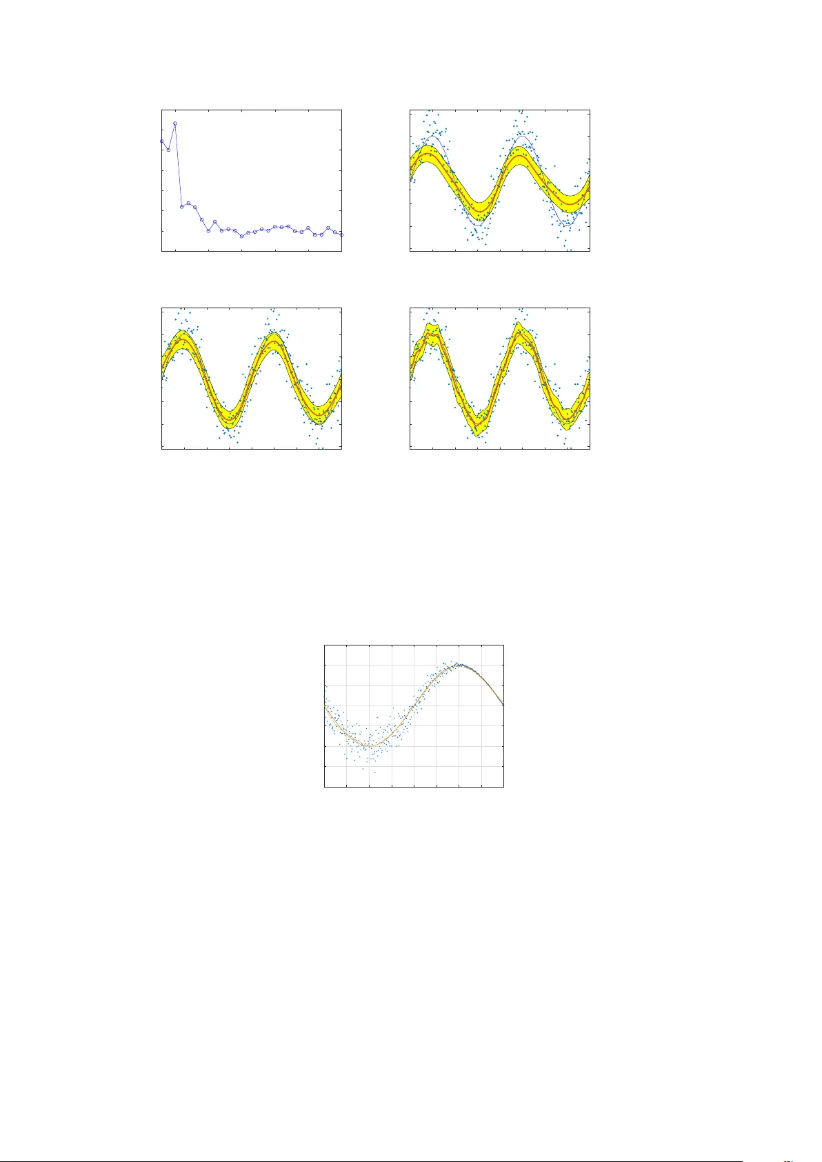
W eigh ted Quasi In terp olan t Spline Appro ximations: Prop erties and Applications Andrea Raffo 1,2,3 and Silvia Biasotti 3 1 Dep artment of Mathematics and Cyb ernetics, SINTEF, Oslo, Norway. 2 Dep artment of Mathematics, University of Oslo, Oslo, Norway. 3 Istituto di Matematic a Applic ata e T e cnolo gie Informatiche “E. Magenes” CNR, Genova, Italy. Abstract Con tinuous represen tations are fundamen tal for modeling sampled data and per- forming computations and numerical simulations directly on the model or its ele- men ts. T o effectiv ely and efficiently address the approximation of p oin t clouds w e prop ose the W eigh ted Quasi Interpolant Spline Approximation method (w QISA). W e provide global and lo cal b ounds of the metho d and discuss how it still preserves the shape prop erties of the classical quasi-in terp olation sc heme. This approac h is particularly useful when the data noise can b e represen ted as a probabilistic distri- bution: from the p oin t of view of nonparametric regression, the wQISA estimator is robust to random p erturbations, suc h as noise and outliers. Finally , w e sho w the effectiv eness of the method with sev eral numerical sim ulations on real data, including curv e fitting on images, surface approximation and sim ulation of rainfall precipitations. Keyw ords : Spline metho ds, quasi-in terp olation, non-parametric regression, point clouds, raw data, noise. 1 In tro duction Mo delling sampled data with a contin uous represen tation is essential in many applica- tions suc h as, for instance, image resampling [1], geometric mo delling [2], isogeometric analysis (IgA) [3] and the n umerical solution of PDE b oundary problems [4]. Spline interpolation is largely adopted to appro ximate data from a function or a ph ysical ob ject b ecause of the simplicit y of its construction, its ease and accuracy of ev aluation, and its capacity to approximate complex shap es through mathematical ele- men t fitting and in teractive design [5]. It is often preferred to p olynomial in terp olation b ecause it yields visually effectiv e results ev en when using low degree p olynomials, while a voiding the Runge’s phenomenon for higher degrees [6]. B-splines represen t a p opular w ay for dealing with spline in terp olation and are no w adays the most p o w erful tool in CA GD [7]. Sev eral generalizations to non-p olynomial splines are possible, such as gen- eralized splines [8], which admit also trigonometric or exp onen tial bases, or non-uniform rational B-splines (NURBS) [9]. The B-spline extension to higher dimensions consists of m ultiv ariate spline functions based on a tensor pro duct approach. Unfortunately , clas- sical tensor pro duct splines lack lo cal refinement, which is often fundamental in those applications dealing with large amoun ts of data. F or this reason several alternative structures that supp ort lo cal refinement hav e been introduced in the last decades; for instance, in the context of a tensor-pro duct paradigm, T-splines [10], hierarc hical B- splines [11], locally refined (LR) B-splines [12] and (truncated) Hierarchical B-splines (THB) [13]. 1 When dealing with real data – for instance, acquired by laser scanners, photogram- metry and diagnostic devices – there are man y source of uncertaint y , such as resolution, precision, occlusions and reflections. F urthermore, digital models often undergo p ost- pro cessing stages after acquisition, and these may in tro duce additional geometric and/or n umerical artefacts [14]. Most of the existing in v erse appro ximation tec hniques are exe- cuted as a deterministic problem and the parameters inv olv ed in the mo del are treated as unambiguous v alues. Despite the recen t in tro duction of uncertain ty-based in verse analysis to ols such as evidence-theory , fuzzy and in terv al uncertainties [15], at the b est of our knowledge, only few modelling approaches iden tify uncertaint y theories as a go od solution for explicitly mo delling data uncertain ty , adopting, for instance, interpro xima- tion [16] or fuzzy num b ers [17]. Unfortunately , these efforts w ere quite isolated and their computational complexity prev ented their massive adoption. In this scenario, w e aim at preserving the use of B-spline bases b ecause of their simplicit y , their approximation capabilit y and accuracy . T o effectively and efficien tly appro ximate ra w data and p oin t clouds possibly affected by noise and outliers, w e pro- p ose the adoption of a nov el quasi-interpolation scheme. Quasi-in terp olation is a well kno wn tec hnique [18, 19] that does not require to solv e an y linear system, unlike the traditional spline approaches, and therefore it allo ws to define more efficient algorithms. Whilst there are works on the use of quasi-interpolant metho ds for function approxima- tion [18, 20, 21, 22, 23, 24], to the b est of our knowledge, less efforts hav e b een devoted to define quasi-in terp olan t schemes for p oin t clouds [25, 26, 27, 28]. As w orking assumptions, we assume the point cloud to b e em b edded in an Euclidean space R d +1 and lo cally represen ted as a heigh t field y = f ( x 1 , . . . , x d ). W e obtain a metho d whic h is not only robust, but also has a reduced computational complexity thanks to the adopted quasi-in terp olation scheme. The metho d prop erties, presen ted in detail for the uni- and biv ariate cases for simplicity of notation, can be easily extended to consider data of arbitrary dimension. W e also discuss how the shape properties of monotonicit y and conv exit y derive from classical spline theory . Since we aim at address- ing data affected b y noise, we pro vide a probabilistic interpretation of the method. W e illustrate its properties ov er a num b er of examples, ranging from curv e fitting to the appro ximation of scalar fields defined on surfaces. In summary , the main contributions of this w ork are: • The in tro duction of a nov el quasi-in terp olation scheme to approximate p oin t clouds, p ossibly affected b y noise and outliers, together with a theoretical study of its n u- merical prop erties (Section 2). • The interpretation of our approac h in terms of the nonparametric regression scheme, together with the theoretical study of bias and v ariance of the wQISA estimator (Section 3). • The v alidation of the metho d on real data from different applications, including curv e fitting, surface reconstruction and rainfall approximation and forecasting (Section 4). Finally , concluding remarks are provided in Section 5. 2 W eigh ted quasi-in terp olan t spline approximation for p oin t clouds In this Section we first summarise some basic notation and definitions on B-splines. W e then formally introduce the weigh ted quasi-in terp olan t spline approximations, pro- vide their global and local bounds and discuss in what sense they preserv e the shap e prop erties. 2 2.1 Basic concepts on spline spaces F rom B-splines theory , it is well known that a non-decreasing sequence t = [ t 1 , . . . , t n + p +1 ], whic h is commonly referred to as glob al knot ve ctor , generates n B-splines of degree p o ver t . In practice, the construction of each of these B-splines requires only a subsequence of p + 2 consecutive knots, collected in a lo c al knot ve ctor . Definition 2.1 (Univ ariate B-spline) . Let t := [ t 1 , . . . , t p +2 ] b e a (lo cal) knot vector. A B-spline B [ t ] : R → R of degree p is the function recursiv ely defined b y B [ t ]( x ) := x − t 1 t p +1 − t 1 B [ t 1 , . . . , t p +1 ]( x ) + t p +2 − x t p +2 − t 2 B [ t 2 , . . . , t p +2 ]( x ) , (1) where B [ t i , t i +1 ]( x ) := ( 1 , if x ∈ [ t i , t i +1 ) 0 , elsewhere , i = 1 , . . . , p + 1 . Here, the con v ention is assumed that “0 / 0 = 0”. By assuming t 1 < t p +2 , it follows that B [ t ] is a piecewise polynomial of degree p . The contin uit y at each unique knot is p − m , where m is the num b er of times the knot is rep eated. B [ t ] is smooth in eac h open subinterv al ( t i , t i +1 ), where i = 1 , . . . , p + 1, and is non-negative ov er R . The supp ort of B [ t ], i.e., the closure of the subset of the domain where B [ t ] is non-zero, is the compact in terv al supp( B [ t ]) = [ t 1 , t p +2 ]. Definition 2.2 (Univ ariate spline space) . Given a global knot vector t = [ t 1 , . . . , t n + p +1 ], the spline sp ac e S p, t is the linear space defined b y S p, t := span n B [ t (1) ] , . . . , B [ t ( n ) ] o , where t ( i ) := [ t i , . . . , t i + p +1 ] for an y i = 1 , . . . , n . An element f ∈ S p, t is called a spline function , or just a spline , of degree p with knots t . By assuming that no knot o ccurs more than p + 1 times, it follows that  B [ t ( i ) ]  n i =1 is a basis for S p, t . A B-spline basis forms a partition of unity ov er [ t 1 , t n + p +1 ]. W e can refine a spline curve f = P n i =1 b i B [ t ( i ) ] b y inserting new knots in t and then computing the coefficients of f in the augmen ted spline space. An efficien t wa y to perform this pro cess is the Oslo algorithm [29]. Lastly , we specify the type of knot vectors w e will consider in the next sections, as they allow to define B-spline bases that interpolate the b oundaries. Definition 2.3. A knot v ector t = [ t 1 , . . . , t n + p +1 ] is said to b e ( p + 1) -r e gular if 1. n ≥ p + 1, 2. t 1 = t p +1 and t n +1 = t n + p +1 , 3. t j < t j + p +1 for j = 1 , . . . , n . Definition 2.4 (T ensor pro duct B-spline) . A tensor pr o duct B-spline of m ulti-degree p := ( p 1 , . . . , p d ) ∈ N d is a separable function B : R d → R defined as B [ t 1 , . . . , t d ]( x ) := d Y k =1 B [ t k ]( x k ) , (2) where x = ( x 1 , . . . , x d ) and t k = [ t k, 1 , . . . , t k,p k +2 ] ∈ R p k +2 is the lo cal knot vector along x k , for an y k = 1 , . . . , d . 3 By assuming that t k, 1 < t k,p k +2 for any k = 1 , . . . , d , it follows that B [ t 1 , . . . , t d ] is a piecewise p olynomial of multi-degree p . Definition 2.5 (T ensor product spline space) . A tensor pr o duct spline sp ac e S p , [ t 1 ,..., t d ] is the linear space defined b y S p , [ t 1 ,..., t d ] := d O k =1 S p k , t k = span ( d Y k =1 B [ t ( i k ) k ] s.t. i k = 1 , . . . , n k ) , where t k ∈ R n k + p k +1 is a global knot vector for any k = 1 , . . . , d . An element f ∈ S p , [ t 1 ,..., t d ] is called a tensor pr o duct spline function, or just a spline , of multi-degree p with knot v ectors t 1 , . . . , t d . The tensor pro duct spline representation inherits all the prop erties (lo cal supp ort, non-negativit y , lo cal smo othness, partition of unity) of the univ ariate case. W e refer the reader to [5] for a more exhaustiv e in tro duction to B-splines. 2.2 W eighted Quasi In terp olation Spline Approximation W e introduce our metho d for the general case of a p oin t cloud P ⊂ R d +1 . Again, w e assume that the p oin t cloud can b e lo cally represen ted by means of a function y = f ( x 1 , . . . , x d ) . Definition 2.6. Let P ⊂ R d +1 b e a p oin t cloud and p ∈ N d a (multi)-degree with all nonzero components. Let t k ∈ R n k + p k +1 b e a ( p k + 1)-regular knot v ector with b oundary knots t p k = a k and t n k +1 = b k , for k = 1 , . . . , d . The Weighte d Quasi Interp olant Spline Appr oximation (wQISA) of degree p to the p oin t cloud P ov er the knot vectors t k is defined by f w := n 1 X i 1 =1 . . . n d X i d =1 ˆ y w  ξ ( i 1 ) 1 , . . . , ξ ( i d ) d  · B [ t ( i 1 ) 1 , . . . , t ( i d ) d ] , (3) where ξ ( i k ) k := ( t k,i k +1 + . . . + t k,i k + p k ) /p k are the knot aver ages and ˆ y w ( u ) := P ( x 1 ,...,x d ,y ) ∈P y · w u ( x 1 , . . . , x d ) P ( x 1 ,...,x d ,y ) ∈P w u ( x 1 , . . . , x d ) (4) are the c ontr ol p oints estimators of weight functions w u : R d → [0 , + ∞ ). The function w u : R d → [0 , + ∞ ) of Definition 2.6 defines a window around eac h p oin t u ∈ R d and is also called a Parzen window . An example is the weigh t function: w u ( x ) := ( 1 /k , if x ∈ N k ( u ) 0 , otherwise , (5) where k ∈ N ∗ and N k ( u ) denotes the neighborho o d of u defined by the k closest p oin ts of the p oint cloud. In this case, ˆ y w defines the k -nearest neigh b or ( k -NN) regressor (see figure 1). Commonly , the function w u dep ends on a distance, for examples: w u ( x ) = 1 || x − u || 2 ≤ r (Characteristic) (6a) w u ( x ) = e −|| x − u || 2 / 2 σ 2 (Gaussian) (6b) w u ( x ) = e −|| x − u || 2 / √ 2 σ (Exp onen tial) (6c) Note that: 4 -2 -1 0 1 2 3 4 -7 -6 -5 -4 -3 -2 -1 0 1 2 3 Figure 1: Parzen windo ws and control p oin ts estimators. Giv en a 2D point cloud (in blue), we compute ˆ y w at u = 1 (in green) b y using the 10 nearest p oin ts (in red). • w u dep ends on the point u ∈ R d of in terest, and can thus be adapted to lo cal information (e.g., v ariable level and/or nature of noise). • The quality of an approximation strongly dep ends on the spline space and the w eight functions that are chosen in Definition 2.6. As sho wn in Figure 2, a giv en spline space and weigh t function is not alw a ys able to capture the relev an t trends of a point set. (a) (b) (c) Figure 2: wQISA curve appro ximation of three p oin t clouds. The p oin t sets (in blue) are sampled from y = sin ( π x ) in (a), y = sin (2 π x ) in (b) and y = sin (3 π x ) in (c) and then p erturb ed with Gaussian noise and outliers. Here, we consider a spline space of dimension 10 o ver a uniform knot vector and a Gaussian weigh t function (see Equation (6b)) of fixed v ariance, combined with quartiles to filter the outliers. The figures shows the original functions (in orange) and the approximations (in red). 2.3 Prop erties W e first in tro duce b ounds for the wQISA appro ximation. W e then explain in what sense shap e prop erties (monotonicity and conv exity) are preserved in case of ra w data. While w e refer the reader to App endix A for a detailed in tro duction of the univ ariate case, here, w e fo cus our atten tion on the biv ariate setting, i.e., on represen tations of the form z = f ( x, y ). The extension of these results to higher dimensions is straightforw ard and just requires a more inv olved notation. F or the sak e of simplicit y , w e re-write Equation (3) as f w ( x, y ) := n x X i =1 n y X j =1 ˆ z w  ξ ( i ) x , ξ ( j ) y  · B [ x ( i ) , y ( j ) ]( x, y ) , where we customize the notation by denoting with ξ ( i ) x (resp. ξ ( j ) y ) the i -th (resp. j -th) knot av erage with resp ect to the global knot vector x (resp. y ) along x (resp. y). 5 2.3.1 Global and lo cal b ounds Prop osition 2.1 (Global b ounds) . L et P ⊂ R 3 b e a p oint cloud. Given z min , z max ∈ R that satisfy z min ≤ z ≤ z max , for al l ( x, y , z ) ∈ P , then the weighte d quasi interp olant spline appr oximation to P fr om some spline sp ac e S p, [ x , y ] and some family of weight functions w u : R 2 → [0 , + ∞ ) has the same b ounds z min ≤ f w ( x, y ) ≤ z max , for al l ( x, y ) ∈ R 2 . Pr o of. F rom the partition of unity of a B-spline basis, it follo ws that min i ˆ z w ( ξ ( i ) x , ξ ( j ) y ) ≤ n x P i =1 n y P j =1 ˆ z w ( ξ ( i ) x , ξ ( j ) y ) · B [ x ( i ) , y ( j ) ] ≤ max i ˆ z w ( ξ ( i ) x , ξ ( j ) y ) ≥ 1 =: ≤ 2 z min f w z max (7) where the inequalities 1 and 2 are a direct consequence of defining ˆ z w b y means of a con vex com bination. The b ounds of Prop osition 2.1 can p otentially lead to lo cal b ounds, for example when the weigh t functions hav e b ounded supp ort. W e discuss this p ossibilit y in Corollary 2.2. Corollary 2.2 (Lo cal b ounds) . L et P ⊂ R 3 b e a p oint cloud. L et x ∈ [ x µ , x µ +1 ) for some µ in the r ange p x + 1 ≤ µ ≤ n x and y ∈ [ y ν , y ν +1 ) for some ν in the r ange p y + 1 ≤ ν ≤ n y . Then α ( µ, ν ) ≤ f w ( x, y ) ≤ β ( µ, ν ) for some α ( µ, ν ) , β ( µ, ν ) which b elong to [ z min , z max ] . Pr o of. By using the prop ert y of lo cal supp ort for B-splines, it follo ws that f w ( x, y ) = µ X i = µ − p x ν X j = ν − p y ˆ z w ( ξ ( i ) x , ξ ( j ) y ) B [ x ( i ) , y ( j ) ]( x, y ) . Hence min i = µ − p x ,...,µ j = ν − p y ,...,ν ˆ z w ( ξ ( i ) x , ξ ( j ) y ) ≤ f w ( x, y ) ≤ max i = µ − p x ,...,µ j = ν − p y ,...,ν ˆ z w ( ξ ( i ) x , ξ ( j ) y ) ≥ 3 ≤ 4 min n z s.t. ( x, y , z ) ∈ P µ,ν o max n z s.t. ( x, y , z ) ∈ P µ,ν o =: =: α ( µ, ν ) β ( µ, ν ) (8) where P µ,ν := S i = µ − p x ,...,µ j = ν − p y ,...,ν supp  w ( ξ ( i ) x ,ξ ( j ) y )  ∩ P and where supp denotes the supp ort of a function. The inequalities 3 and 4 are a direct consequence of defining ˆ z w b y means of a conv ex com bination. Note that the set P ∗ of p oin ts that are effectively used to compute the approximation, i.e., P ∗ := [ µ = p x +1 ,...,n x ν = p y +1 ,...,n y P µ,ν , ma y be a prop er subset of P . 6 Note also that the results of Prop osition 2.1 and Corollary 2.2 are indep enden t from the t yp e of mesh but rather rely on the partition of unit y prop ert y . Therefore, a p ossibilit y is to consider lo cal refinement strategies in order to further reduce the computational complexity and gain more flexibilit y only where truly needed. 2.3.2 Shape preserv ation Shap e preserving representations are crucial in geometric mo deling (e.g., in CAD and CAM). Man y classical quasi-in terp olan t strategies for function appro ximation preserve shap e prop erties, suc h as the Bernstein appro ximants, the B-spline or multiquadratic (MQ) quasi-interpolants, the V ariation Diminishing Spline Appro ximation (VDSA) and so on [30, 22, 31, 32]. In case of p oin ts clouds with defects, the av erage dataset trend is more important than the p osition of a single p oin t with resp ect to the others. W e th us introduce a notion of monotonicit y and conv exit y for p oin t clouds that tak e this consideration in to accoun t. Given a family of weigh t functions, we sa y that a p oin t cloud is w-monotone (resp. w-c onvex ) if the control p oin t estimator ˆ z w is monotone (resp. con vex) (see App endix A for a formal definition). Monotonicit y and conv exity of the individual co ordinates are preserv ed from w - monotonicit y and w -con v exity as a direct consequence of the univ ariate case, which is detailed in Appendix A. More precisely: • (Monotonicity) Let us supp ose that ˆ z w ( · , y 0 ) : R → R is monotonic for all y 0 ∈ [ a 2 , b 2 ] (or at least it is its restriction to the no des { ξ ( i ) x } n x i =1 ). Then, f w is an in- creasing function of x for each y . This statemen t is formally prov ed in Prop osition A.4. • (Convexity) Let us supp ose that ˆ z w ( · , y 0 ) : R → R is conv ex for all y 0 ∈ [ a 2 , b 2 ] (or at least it is its restriction to the no des { ξ ( i ) x } n x i =1 ). Then, f w is a conv ex function of x for eac h y . This statement is formally prov ed in Prop osition A.6. In the multiv ariate setting, join t monotonicit y and con vexit y straigh tforwardly deriv e from the control net shap e [33, 31], here defined b y ˆ z w . More precisely , a w -monotone (resp. w -con vex) p oin t cloud has a monotone (resp. conv ex) wQISA approximation. 2.3.3 Computational complexity The wQISA metho d tak es as input the p oin t cloud P ⊂ R d +1 , the tensor pro duct spline space S p , [ t 1 ,..., t d ] defined b y a m ulti-degree and a set of regular knot v ectors, and the P arzen windo w function w . The approximation defined by Equation (3) is computed by ev aluating Equation (4) as many times as the dimension of the tensor product spline space, i.e., dim( S p , [ t 1 ,..., t d ] ) = Q d i =1 n i . The single con trol p oin t estimation dep ends on the function w c hosen and, in par- ticular, on its supp ort (if global or lo cal). In the n umerical sim ulations prop osed in Section 4, we mainly fo cus on k-NN and In verse Distance W eight (ID W) functions (see Equations (5) and (20)) and, therefore, we here exhibit the computational complexity of wQISA for these choices of w . A deep en study of the computational complexity can b e found in [34]. The k -nearest neighbor can b e efficiently computed using the k -d tree algorithm in O ( N log( N )) op erations [35], where N is the n umber of p oin ts of the cloud. The k -d tree then spatially stores the data in a structure such that, at runtime, the ev aluation of w costs O ( k ). Thus, the computation cost of the wQISA algorithm is given by the maxim um of O ( N log( N )) and O ( k · dim( S p , [ t 1 ,..., t d ] )). The IDW weigh t is global and thus computes, for a single con trol p oint estimation, the linear com bination of N terms. Since computing the w eigh t of an y point is at most as 7 exp ensiv e as the inv erse of an Euclidean norm, the computational complexity is O ( N d ). The computational cost of the wQISA algorithm is then O ( N · dim( S p , [ t 1 ,..., t d ] ))). 3 The wQISA metho d from a probabilistic p ersp ectiv e Regression analysis techniques are widely used for prediction and forecasting. In regres- sion problems, the conditional expectation of a resp onse v ariable Y with resp ect to its predictor v ariables X 1 , . . . , X p is often approximated b y its first-order T a ylor expansion. Linearit y in the predictors leads to a m uc h easier interpretabilit y of the mo del and is v ery efficien t with sparse and small data. Global and local least square approaches are among the most p opular linear regression metho ds. Nev ertheless, these mo dels need to solve linear systems of equations, whic h thus unnecessarily increases computational complexit y as the data size increases. Moreo ver, linear models often dep end on the nor- mal distribution of the residuals, making them unreliable when the actual distribution is asymmetric or prone to outliers. As the assumption of linearit y might b e too restrictiv e for real-world phenomena, v arious metho ds for mo ving b ey ond it hav e b een in tro duced. A p opular approac h, kno wn as line ar b asis exp ansion , considers multiple transformations of the predictors and then applies linear mo dels in this richer space. Compared to traditional linear mo dels, p oly- nomial transformations of the predictors offer a more flexible data representation as they lead to higher-order T aylor expansions. On the other hand, they suffer a lack of lo cal shape control due to their global nature. Compared to p olynomial bases, piecewise p olynomials allo w to combine an increased flexibilit y with a reduced num b er of co effi- cien ts to compute. F urthermore, nonparametric regression ma y b e used for a v ariet y of purp oses, suc h as scatterplot smo othing for pure exploration and in terv al estimates for uncertain ty examination [36]. As we theoretically and numerically sho w in Sections 3 and 4, the wQISA metho d offers a comp etitiv e alternative to handle strongly p erturb ed large p oin t clouds at a reduced computational cost, even when prone to outliers. In this Section we in terpret the WQISA metho d as a non parametric regression problem. Indep enden t ongoing studies on quasi-in terp olation from a sto chastic persp ectiv e are in [37, 38]. 3.1 F ormulation of the regression problem Let Y be a univ ariate resp onse v ariable. F or the sake of simplicit y , we restrict here to t wo predictor v ariables X 1 and X 2 . As for the previous sections, the generalization to the multiv ariate case is trivial and just requires only a more inv olved notation. F rom no w on, w e assume that the relationship b et ween the predictors and the dep enden t v ariable can b e expressed as the conditional exp ectation: E ( Y | X 1 = x 1 , X 2 = x 2 ) = f w ( x 1 , x 2 ) . The approximation f w is here restricted to b elong to a subspace of S p , [ x 1 , x 2 ] , where p ∈ N ∗ × N ∗ is the (bi)-degree of the spline space ov er the (global) knot vectors x 1 and x 2 . More precisely , the relation b et w een the observ ations Y i and the indep enden t v ariables X i, 1 and X i, 2 is formulated as Y i = n 1 X j 1 =1 n 2 X j 2 =1 c j 1 ,j 2 B [ x ( j 1 ) 1 , x ( j 2 ) 2 ]( X i, 1 , X i, 2 ) + ε i , i = 1 , . . . , N , (9) where • B [ x ( j 1 ) 1 , x ( j 2 ) 2 ] : R 2 → [0 , 1] is the ( j 1 , j 2 )-th tensor pro duct B-spline function with resp ect to the global knot vectors x 1 and x 2 resp ectiv ely along X 1 and X 2 . 8 • ε i is the residual or disturbance term – an unobserv ed random v ariable that per- turbs the linear relationship b et ween the dep enden t v ariable and regressors. Relation (9) can b e expressed, up to a reordering of the indexes ( j 1 , j 2 ), in the matrix form Y = B · c + ε , (10) where Y ∈ R N × 1 3 ε , B ∈ R N × ( n 1 · n 2 ) and c ∈ R ( n 1 · n 2 ) × 1 . 3.2 Definition of the co efficien t estimators There are different methods to fit a linear mo del to a given dataset. In the following, w e in tro duce our new estimators for the B-spline coefficients. The ( j 1 , j 2 )-th comp onen t of ˆ c is defined b y ˆ c j 1 ,j 2 := N P i =1 Y i · w ( ξ ( j 1 ) 1 ,ξ ( j 2 ) 2 ) ( X i, 1 , X i, 2 ) N P i =1 w ( ξ ( j 1 ) 1 ,ξ ( j 2 ) 2 ) ( X i, 1 , X i, 2 ) , (11) where ξ ( j 1 ) 1 and ξ ( j 2 ) 2 are the knot aver ages with respect to the B-spline B j 1 ,j 2 along the t wo directions. Notice that the weigh t functions w ( ξ ( j 1 ) 1 ,ξ ( j 2 ) 2 ) : R 2 → [0 , + ∞ ) act b oth as a p enalt y term and as a smo other on the giv en data. 3.3 Inference for regression purp oses: the bias-v ariance decomp osition Supp ose the data arise from a model Y = f ( X 1 , X 2 ) + ε . F or the sak e of simplicit y , w e assume here that the v alues of the predictors are fixed in adv ance, hence nonrandom. F urther, w e assume the error terms ε i to b e indep endent identic al ly distribute d (i.i.d) with mean µ ε = 0 and v ariance σ 2 ε . The generalization p erformances of a metho d relies on the simultaneously minimiza- tion of t w o sources of error: • The bias measures the difference b et ween the mo del’s exp ected predictions and the true v alues. High bias means an ov ersimplification of the mo del, i.e., the mo del do es not produce accurate predictions (underfitting). The bias of a mo del is formally defined b y Bias 2 h ˆ f w ( X 1 , X 2 ) i :=  E h ˆ f w ( X 1 , X 2 ) i − f ( X 1 , X 2 )  2 . (12) • The varianc e measures the mo del’s sensitivit y to small fluctuations in the training set. High v ariance can result in a mo del that interpolates the giv en data but do es not generalize on data which hasn’t seen b efore (ov erfitting). The v ariance of a mo del is defined by V ar h ˆ f w ( X 1 , X 2 ) i := E   ˆ f w ( X 1 , X 2 ) − E h ˆ f w ( X 1 , X 2 ) i 2  . (13) 3.3.1 Bias of a wQISA mo del Let ( X 1 , X 2 ) ∈ [ x 1 ,µ , x 1 ,µ +1 ) × [ x 2 ,ν , x 2 ,ν +1 ) for some µ = p 1 + 1 , . . . , n 1 and for some ν = p 2 + 1 , . . . , n 2 . By using the property of lo cal supp ort of B-splines, we can then express E [ ˆ f w ( X 1 , X 2 )] as E [ ˆ f w ( X 1 , X 2 )] = µ X j 1 = µ − p 1 ν X j 2 = ν − p 2 E [ˆ c j 1 ,j 2 ] · B [ x ( j 1 ) 1 , x ( j 2 ) 2 ]( X 1 , X 2 ) , (14) 9 where E  ˆ c j 1 ,j 2  = N P i =1 f ( X i, 1 , X i, 2 ) · w ( ξ ( j 1 ) 1 ,ξ ( j 2 ) 2 ) ( X i, 1 , X i, 2 ) N P i =1 w ( ξ ( j 1 ) 1 ,ξ ( j 2 ) 2 ) ( X i, 1 , X i, 2 ) (15) is a con vex combination. Once a s pline space and weigh t functions ha ve b een c hosen, Equations (14) and (15) can b e combined to write do wn the exact form ula of bias. Ho wev er, in some cases b ounds can simplify its study . Analogously to Proposition 2.1, w e can compute the follo wing b ounds for E  ˆ c j 1 ,j 2  min i ∈I ˆ c j 1 ,j 2 f ( X i, 1 , X i, 2 ) ≤ E  ˆ c j 1 ,j 2  ≤ max i ∈I ˆ c j 1 ,j 2 f ( X i, 1 , X i, 2 ) , (16) where I ˆ c j 1 ,j 2 := n i = 1 , . . . , N s.t. w ( ξ ( j 1 ) 1 ,ξ ( j 2 ) 2 ) ( X i, 1 , X i, 2 ) 6 = 0 o . By combining Equations (14) and (16), it follows that min i ∈I µ,ν f ( X i, 1 , X i, 2 ) ≤ µ P j 1 = µ − p 1 ν P j 2 = ν − p 2 E  ˆ c j 1 ,j 2  B [ x ( j 1 ) 1 , x ( j 2 ) 2 ]( X 1 , X 2 ) ≤ max i ∈I µ,ν f ( X i, 1 , X i, 2 ) =: =: =: α ( µ, ν ) E  ˆ f w ( X 1 , X 2 )  β ( µ, ν ) (17) where I µ,ν := [ j 1 = µ − p 1 ,...,µ j 2 = ν − p 2 ,...,ν I ˆ c j 1 ,j 2 and where α and β denote the low er and upp er b ounds. W e conclude that Bias 2 h ˆ f w ( X 1 , X 2 ) i ( ≤  α ( µ, ν ) − f ( X 1 , X 2 )  2 , if E  ˆ f w ( X 1 , X 2 )  ≤ f ( X 1 , X 2 ) ≤  β ( µ, ν ) − f ( X 1 , X 2 )  2 , if E  ˆ f w ( X 1 , X 2 )  ≥ f ( X 1 , X 2 ) , (18) where α ( µ, ν ) and β ( µ, ν ) denote the minim um of maxim um in Equation (17). 3.3.2 V ariance of a wQISA mo del In the follo wing Lemma w e pro vide an exact form ula for the v ariance while pro ving that, in the w orst p ossible case, the v ariance will still b e upp er bounded by σ 2 ε . F or the sak e of simplicit y , w e consider a reordering of B-splines as in Equation (10). This choice allows to substitute the indexes ( j 1 , j 2 ) with a single index j . Lemma 3.1. The varianc e of ˆ f w is upp er-b ounde d by the varianc e of the err or, i.e., V ar h ˆ f w ( X 1 , X 2 ) i ≤ σ 2 ε . 10 Pr o of. V ar h ˆ f w ( X 1 , X 2 ) i = E   ˆ f w ( X 1 , X 2 ) − E  ˆ f w ( X 1 , X 2 )   2  = = E   X i ˆ c i B i ( X 1 , X 2 ) − X i E [ ˆ c i ] B i ( X 1 , X 2 ) ! 2   = = E   X i ( ˆ c i − E [ ˆ c i ]) B i ( X 1 , X 2 ) ! 2   = = X i X j E [( ˆ c i − E [ ˆ c i ]) ( ˆ c j − E [ ˆ c j ])] B i ( X 1 , X 2 ) B j ( X 1 , X 2 ) = = X i X j Co v ( ˆ c i , ˆ c j ) B i ( X 1 , X 2 ) B j ( X 1 , X 2 ) , where Co v ( ˆ c i , ˆ c j ) = Co v P k 1 Y k 1 · w ( ξ ( i ) 1 ,ξ ( i ) 2 ) ( X k 1 , 1 , X k 1 , 2 ) P k 1 w ( ξ ( i ) 1 ,ξ ( i ) 2 ) ( X k 1 , 1 , X k 1 , 2 ) , P k 2 Y k 2 · w ( ξ ( j ) 1 ,ξ ( j ) 2 ) ( X k 2 , 1 , X k 2 , 2 ) P k 2 w ( ξ ( j ) 1 ,ξ ( j ) 2 ) ( X k 2 , 1 , X k 2 , 2 ) ! = = P k 1 P k 2 w ( ξ ( i ) 1 ,ξ ( i ) 2 ) ( X k 1 , 1 , X k 1 , 2 ) · w ( ξ ( j ) 1 ,ξ ( j ) 2 ) ( X k 2 , 1 , X k 2 , 2 ) Co v ( Y k 1 , Y k 2 ) P k 1 P k 2 w ( ξ ( i ) 1 ,ξ ( i ) 2 ) ( X k 1 , 1 , X k 1 , 2 ) · w ( ξ ( j ) 1 ,ξ ( j ) 2 ) ( X k 2 , 1 , X k 2 , 2 ) = = σ 2 ε P k 1 w ( ξ ( i ) 1 ,ξ ( i ) 2 ) ( X k 1 , 1 , X k 1 , 2 ) · w ( ξ ( j ) 1 ,ξ ( j ) 2 ) ( X k 1 , 1 , X k 1 , 2 ) P k 1 P k 2 w ( ξ ( i ) 1 ,ξ ( i ) 2 ) ( X k 1 , 1 , X k 1 , 2 ) · w ( ξ ( j ) 1 ,ξ ( j ) 2 ) ( X k 2 , 1 , X k 2 , 2 ) . Th us V ar h ˆ f w ( X 1 , X 2 ) i = X i X j Co v ( ˆ c i , ˆ c j ) B i ( X 1 , X 2 ) B j ( X 1 , X 2 ) = = σ 2 ε X i X j P k 1 w ( ξ ( i ) 1 ,ξ ( i ) 2 ) ( X k 1 , 1 , X k 1 , 2 ) · w ( ξ ( j ) 1 ,ξ ( j ) 2 ) ( X k 1 , 1 , X k 1 , 2 ) P k 1 P k 2 w ( ξ ( i ) 1 ,ξ ( i ) 2 ) ( X k 1 , 1 , X k 1 , 2 ) · w ( ξ ( j ) 1 ,ξ ( j ) 2 ) ( X k 2 , 1 , X k 2 , 2 ) · · B i ( X 1 , X 2 ) B j ( X 1 , X 2 ) ≤ σ 2 ε , where the inequalit y holds because B i B j has the partition of unity prop ert y . In Lemma 3.1, the exact expression of the v ariance mak es it p ossible to compute exact and appro ximated (p oin twise) standard error bands (see Equation (19)). 3.3.3 Bias-v ariance decomp osition for the k -NN w eight Let’s consider an example to sho w ho w the results of the section work in practice. Let w b e a k -NN w eight function (see Equation (5)). The exact expression of the bias is found by com bining Equation (12) with the exp ected v alue E [ ˆ f w ( X 1 , X 2 )] = 1 k µ X j 1 = µ − p 1 ν X j 2 = ν − p 2 B [ x ( j 1 ) 1 , x ( j 2 ) 2 ]( X 1 , X 2 ) · · X ( X i, 1 ,X i, 2 ) ∈ N k ( ξ ( j 1 ) 1 ,ξ ( j 2 ) 2 ) f ( X i, 1 , X i, 2 ) . The exact expression of v ariance is given b y V ar h ˆ f w ( X 1 , X 2 ) i = σ 2 ε X i X j k i,j k 2 · B i ( X 1 , X 2 ) B j ( X 1 , X 2 ) ≤ σ 2 ε k , 11 where k i,j is the num b er of p oin ts in common, if any , among the k -closest to ( ξ ( i ) 1 , ξ ( i ) 2 ) and ( ξ ( j ) 1 , ξ ( j ) 2 ). F or small k , the estimate ˆ f w can potentially adapt itself b etter to the underlying f , as it will av oid p oin ts further aw ay to the knot av erages. Under the assumption of increasing the p oin t cloud size while keeping the sampling uniform, the bias for the 1-NN w eight function v anishes entirely as the size of the training set approaches infinity and the mesh is uniformly refined. On the other hand, larger v alues of k can decrease the v ariance. 3.3.4 Numerical interpretation of the bias-v ariance decomp osition Figure 3 sho ws the effect of spline spaces of different dimensions on the simple example Y = sin π X + ε, with X ∼ U [ − 2 , 2] and ε ∼ N (0 , σ 2 ). Our dataset consists of N = 300 points ( x i , y i ) sampled on the exact curve and then p erturb ed. The weigh ted quasi interpolant spline approximations for three different uniform knot v ectors are sho wn. F or the sake of simplicity , w e here considered a 10-NN w eigh t function. The shaded regions in the figures represent the (p oin twise) standard error band of ˆ f w , i.e., the region ˆ f w ( X ) ± z (1 − α ) · r V ar h ˆ f w ( X ) i , (19) where z (1 − α ) is the 1 − α p ercen tile of the normal distribution. The three approximations displa yed in Figures 3(b-d) give a graphical representation of the bias-v ariance trade-off problem with respect to the dimension of the spline space: n=5 The spline under-fits the data, with a more dramatic bias in those regions with a higher curv ature n=15 Compared to the previous case, the fitted function is closer to the true function. The v ariance has not increased appreciably yet. n=30 The spline o ver-fits the data, which leads to a lo cally increased width of the bands. In practice, the tuning parameters (here: n ) can b e selected via automatic proce- dures, for instance by using the K -fold cross-v alidation, generalized cross-v alidation and the so-called C p statistic [36]. In Figure 3(a) we include the 5-fold cross-v alidation curve C V ( n ) = 1 N N X i =1  y i − ˆ f w ( x i )  2 , where f w dep ends on n via the spline space. Figure 4 shows the appro ximation of a p oint cloud affected b y the non-uniform noise ε ∼ N (0 , s ( X )), defined as follo ws: s ( X ) = e − 1 4(1 + e 4 X − 2 ) . The dataset consists of N = 400 points and is appro ximated b y a spline space con taining n = 15 B-splines ov er a uniform knot vector. 12 5 10 15 20 25 30 n 0 0.1 0.2 0.3 0.4 0.5 0.6 0.7 CV(n) -2 -1.5 -1 -0.5 0 0.5 1 1.5 2 X -1.5 -1 -0.5 0 0.5 1 1.5 y (a) (b) -2 -1.5 -1 -0.5 0 0.5 1 1.5 2 X -1.5 -1 -0.5 0 0.5 1 1.5 y -2 -1.5 -1 -0.5 0 0.5 1 1.5 2 X -1.5 -1 -0.5 0 0.5 1 1.5 y (c) (d) Figure 3: Bias-v ariance tradeoff. In (a) we show the CV(n) curv e for a realization from the c hosen nonlinear additive error model. The minim um is reac hed at n = 15. The remaining panels sho w the data, the true function (in blue), the weigh ted quasi in terp olan t spline approximations (in red) and the (yello w shaded) bands of Equation (19), for spline spaces of dimension n = 5 (b), n = 15 (c) and n = 50 (d). The bands corresp onds here to an appro ximate 95% confidence interv al. -2 -1.5 -1 -0.5 0 0.5 1 1.5 2 X -2 -1.5 -1 -0.5 0 0.5 1 1.5 y Figure 4: V ariable noise approximation. W e show the original curve f ( X ) = sin ( π / 2 · X ) (in red) and the spline approximation (in yello w). 13 4 Numerical simulations W e dra w the effectiv eness of our metho d in a n umber of real data coming from different sources and application domains. While [34] fo cused on the lo cal approximation of 3D p oin t clouds b y wQISA surfaces, this section sho ws ho w the metho d is able to address the appro ximation problem for different dimensions. Indeed, our examples include curv e appro ximation (on images and 3D ob jects), surface appro ximation (of 3D p oin t clouds) and sim ulation of natural phenomena (like rainfall precipitation) o ver surfaces. Unless otherwise stated, w e fo cus here on (bi-)quadratic spline approximations defined o ver uniform knot vectors, as they provide a sufficien t flexibility for our purposes. Neverthe- less, one can consider (bi-)degrees as additional parameters to assess and p erform knot insertion to increase the degrees of freedom only where they are actually needed. 4.1 Ev aluation criteria The data acquisition devices and the subsequen t p ost-processing operations generally in tro duce geometric and numerical artefacts. Unfortunately , for most of the data, the in- formation on the quality of the acquisition devices and t yp e of p ost-processing operations are lost or not av ailable. Therefore, the h yp othesis that the data to be approximated are exact is often unrealistic. Differently from other mo del represen tations, the peculiarity of wQISA is its capability of dealing with data affected b y noise and outliers. This fact reflects on the measuremen ts we can adopt to analyse the qualit y of the data approxi- mation: indeed, it is not imp ortant ho w m uch the wQISA interpolates the original data rather it remains in a reasonable approximation range. T o the b est of our knowledge, a single p erformance measure able to capture suc h complex information do es not exist; therefore, w e will analyse the wQISA output with a num b er of measures, each one able to highlight differen t approximation asp ects. • When N observ ations Y i are appro ximated by ˆ Y i , t wo popular measures of the statistical disp ersion are the Me an Squar e d Err or (MSE) M S E = 1 N N X i =1 ( Y i − ˆ Y i ) 2 and the Me an Absolute Err or (MAE) M AE = 1 N N X i =1 | Y i − ˆ Y i | . Although the MSE and MAE quantities are sample dep enden t and highly affected b y data p erturbation, they offer a v ery in tuitive quan tification of ho w close a point cloud and its appro ximation are. • The Hausdorff distanc e is a well-kno wn distance betw een tw o sets of p oin ts and applies for point clouds in all dimensions. In particular, w e consider the Directed Hausdorff distance [39] from the p oin ts a ∈ A ⊂ R t to the p oin ts b ∈ B ⊂ R t as follo ws: d dH aus ( A, B ) = max a ∈ A min b ∈ B d ( a, b ) , with d the Euclidean distance. In order to ha ve a coherent distance ev aluation through mo dels of different size, we normalize d dH aus with resp ect to the diameter of the point cloud. 14 • The Jac c ar d index (also kno wn as intersection ov er union) quan titatively estimates ho w tw o sets ov erlap. It is has b een previously adopted to measure the p erformance of curv e recognition metho ds for images [40] and 3D models [41]. The Jaccard index b et ween t wo point sets A and B is defined as: J accar d ( A, B ) = | A ∩ B | | A ∪ B | , where | · | denotes here the n umber of elements. The Jaccard index v aries from 0 to 1, the higher the better. In our con text, it can be adapted to the ratio of elemen ts of the original p oin t cloud that lie on the standard error bands of Equation (19). 4.2 Curv e appro ximation W e consider a 512 × 512 axial X-ray CT slice of a human lumbar v ertebra (see Figure 5(a)). First, w e apply an edge detection technique, to detect the set of edge p oints. In this specific example, w e adopt the Canny edge detector [42], others metho ds could b e applied to o. W e select a b ounding b o x for the p oin t cloud, which is then partitioned in smaller sub-regions (see Figure 5(b)). Lastly , w e apply our tec hnique to each sub-region to obtain a global appro ximation (see Figure 5, righ t). Here, a 1-NN w eigh t is set as the num b er of p oin ts is relatively small. Uniform knot v ectors are considered as they pro duce reasonable approximations. The n um b er of B-splines is c hosen, in each sub- region, b y a Leav e-One-Out cross-v alidation [36]. Interpolating conditions are imp osed at the b oundaries in order to ha ve a more natural C 1 con tinuit y (see Figure 5(c)). Notice that the shap e of the vertebra is correctly preserved in the passage from the image to the final appro ximation. (a) (b) (c) Figure 5: X-ra y CT slice. In (a), the original image is shown. Figure (b) displa ys the edge p oin ts and the chosen partition: V1 in green, V2 in red, V3 in blue and V4 in ligh t blue. In (c), the piecewise defined curve is sup erimposed to an enlargement of the original image. Figure 6 shows an example of ey e contour approximation from 3D mo dels. W e consider a fragmen t of a votiv e statue [43] stored in ST AR C rep ository 1 at The Cyprus Institute and extract the ey e con tours b y filtering the point cloud through the v alues of the mean curv ature v alues and clustering [44]. Eac h contour is pro jected onto its regression plane and then lo cally appro ximated. W e here test a k -NN w eight, with k to b e assessed from patch to patch. Knot v ectors are again assumed to b e uniform. F or eac h ey e profile, t wo curv es are detected; the extrema knots of the t wo curv es are fixed to b e the same and are automatically selected as the leftmost and rightmost p oin ts of the whole profile. Notice that with these c hoices our approac h is also able to fill the gaps in a reasonable wa y . 1 h ttp://public.cyi.ac.cy/starcRep o/ 15 (a) (b) -2.5 -2 -1.5 -1 -0.5 0 0.5 1 1.5 2 2.5 -0.5 0 0.5 1 1.5 2 2.5 -2.5 -2 -1.5 -1 -0.5 0 0.5 1 1.5 2 2.5 -0.5 0 0.5 1 1.5 2 2.5 (c) (d) Figure 6: Appro ximation of the ey e contour on a fragmen t of arc haeological artifact. The statue (a) is first prepro cessed to filter the ey e con tours p oin ts (b). Then, each p oin t cloud is lo cally appro ximated. Here the p oints are clustered into: LE1 (left eye, ligh t blue), LE2 (left eye, ligh t purple), RE1 (righ t eye, light blue), RE2 (right ey e, light purple). T able 1 rep orts the v alues of the parameters n and k that b est approximate the original curve segments and the corresp onding error measures for the wQISA appro xi- mations. T able 1: P arameters and accuracy measures for the curve fitting examples. F or eac h cluster of p oin ts we rep ort: the sample size, the n umber of B-splines n , the tuning param- eter k for the k -NN weigh t, the Mean Absolute Error (MAE), the Ro ot Mean Squared Error (RMSE), the Jaccard index and the normalized Hausdorff distance. Parameters with asterisks are set by user. Lum bar V ertebra Left Ey e Righ t Eye V1 V2 V3 V4 LE1 LE2 RE1 RE2 sample size 82 38 30 38 422 730 428 638 n 20 6 8 7 12 12 8 12 k 1 ∗ 1 ∗ 1 ∗ 1 ∗ 5 5 5 5 MAE 0.656 0.3323 0.278 0.292 0.025 0.052 0.025 0.043 RMSE 0.898 0.418 0.378 0.379 0.030 0.074 0.030 0.079 Jaccard 0.988 1.000 1.000 1.000 0.995 1.000 1.000 1.000 Hausdorff 0.014 0.016 0.011 0.012 0.010 0.021 0.017 0.041 4.3 Surface appro ximation A simulation on terrain data is sho wn in Figure 7. The data are part of the Liguria- LAS dataset adopted as testb ed in the iQm ulus pro ject [45], and come from a LID AR dataset with spatial resolution of one meter. The area here selected contains 379.831 p oin ts. It is lo cated in the Liguria region, in the north-west of Italy . The Liguria morphology , with several small catchmen ts and ev en small riv ers, is v ery c hallenging for 16 the appro ximation metho ds to capture and preserve the most imp ortan t and p oten tially critical c haracteristics [46]. The data are obtained with multiple swip es by airplane lidar acquisition. Some p oin ts come from multiple laser p ositions and therefore the same point can hav e m ultiple elev ation v alues. In addition, since the data were only minimally post-pro cessed to conv ert them to .las format, they con tain also noise and outliers. In this example, w e choose a C 1 (bi-)quadratic spline approximation because it is smo oth enough to represen t smooth terrains in a go od w ay . W e consider an In v erse Distance W eight (IDW), defined b y: w ( u,v ) ( x, y ) :=            1 || ( x, y ) − ( u, v ) || 2 , if | C ( u,v ) | = 0    1 | C ( u,v ) | , for all ( x, y ) = ( u, v ) 0 , else , if | C ( u,v ) | 6 = 0 (20) where | C ( u,v ) | := { ( x, y , z ) ∈ P s.t. ( x, y ) = ( u, v ) } . The ID W assigns greater influence to the p oin ts the closest to the knot a verages and hence the most significan t for the terrain approximation. The uniform knot vectors define in the final appro ximation 1024 B-splines in b oth directions and are chosen such that the MSE for the relative punctual error of eac h element is low er than 0 . 05 (which corresp ond to 0.05% of deviation). (a) (b) (c) Figure 7: Portofino, Liguria, Italy . A data point cloud from the giv en region of interest (a) is approximated via an IDW weigh t (b). The colors represent the elev ation and v ary from blue (lo w elev ation) to red (high elev ation). A graphical represen tation of the punctual error, normalized b y the maximum elev ation, is provided in (c). The statistics for the error are: min=0 . 0000, max=0 . 0445, mean=0 . 0021, median=0 . 0017, RMSE=0 . 0029 and std=0 . 0019. The metho d has b een also tested for the approximation of the b oundary of 3D mo dels. As curren tly stated, wQISA is suitable to approximate surface p ortions that can b e represented in a lo cal Cartesian coordinate system in the form z = f ( x, y ). Therefore, 17 the ob ject surface needs a subdivision into charts, for instance following the approaches in [47, 48]. Once the charts hav e b een obtained, w e compute the desired representation adopting as z v alue the height v alue of the c hart with resp ect to its b est fitting regression plane [44]. Figure 8 visually sho w some details of t w o wQISA approximations for 3D p oin ts clouds: the surfaces in the b oxes appro ximate the regions p oin ted b y the (light blue) lines. These models come from the Visionair Shap e Rep ository , VSR [49]. Giv en the low lev el of noise, a pure 1-NN weigh t function is here tested. The approximation sho ws a correct recov ery of the main details of the artefact. Nevertheless, the feeble details are lost as an effect of the smoothing effect of this w eigh t function. (a) (b) Figure 8: Examples on tw o 3D models. F or eac h mo del we highligh t some details of the wQISA approximation computed b y a 1-NN weigh t function. The statistics of the relativ e punctual error are: for the v ase, MSE=4 . 1884 e − 06 and std=0 . 0015; for the curl, MSE=4 . 1493 e − 06 and std=0 . 0016; for the tress, MSE=3 . 7918 e − 05 and std=0 . 0057. 4.4 Appro ximation of surface prop erties As a further case study , w e prop ose the appro ximation of a precipitation even t ov er the Liguria region. T o this purp ose w e consider an even t o ccurred b et ween Jan uary 16 and 20, 2014, whic h w as responsible of heavy rain for ab out fiv e da ys o ver all the Liguria region. The data w e are considering were gathered from rain gauges main tained b y Regione Liguria. The net w ork is spread o v er the whole region, with 143 measure stations. These data come from the use case adopted for the comparison of six rainfall precipitation metho ds in [46]. Here, we compare wQISA with k -NN w eight functions with tw o other methods: ra- dial basis functions (RBF) with Gaussian kernel, as considered in [46], and the Multilevel B-splines Approximation (MBA) [50]. In the RBF implemen tation a global supp ort [51] is adopted (all the 143 rain samples are considered) and a direct solv er is applied to the linear system, whic h is symmetric and p ositiv e-definite. The MBA approximation is obtained with the default settings of the implementation of the Geometry Group at SINTEF Digital, whic h is freely a v ailable at: https://github.com/orochi663/MBA . A quan titative comparison is pro vided in T able 2 and computed by performing 5 times a 5-fold cross-v alidation on each metho d. F or more details, w e refer once again the reader to [36] (chapter 7). The optimal parameters for a k-NN wQISA are chosen b y minimizing the a verage MSE and are: k = 9, with 10 inner knots for each direction. In Figure 9 we sample the precipitation fields appro ximated with the three metho ds in a set of points, represen ting the Liguria region. Although our approximation lo oks smo other and less detailed, it has in practice a b etter generalization p erformance as a learning metho d – that is a b etter prediction capability on indep enden t test data. An implemen tation of the wQISA metho d for rainfall data with the choice of the optimal v alues for the k parameter and the cross-v alidation tests rep orted in T able 2 is freely 18 T able 2: Statistics for the error distribution of the cross v alidation. Metho d Min [mm] Max [mm] Mean [mm] Median [mm] Std [mm] MSE [mm 2 ] RBF 0.0317 2.9363 1.0903 1.0070 0.7830 1.7973 MBA 0.0341 3.3489 1.1667 1.0243 0.8767 2.1969 wQISA 0.0471 2.8293 0.9883 0.9013 0.6885 1.4657 a v ailale at: http s://github.com/rea1991/wQISA. 1 2 3 4 5 6 1 2 3 4 5 (a) (b) (c) Figure 9: Rainfall approximation with RBF (a), MBA (b) and wQISA (c). 5 Concluding remarks and future p ersp ectiv es W e defined a no vel quasi-interpolant reconstruction tec hnique (wQISA), sp ecifically de- signed to handle large and noisy p oin t sets, even when equipp ed with outliers. The robustness and the versatilit y of the metho d are theoretically discussed from the p oin t of view of n umerical analysis (Sections 2.3) and probabilit y theory (Section 3). Numer- ical examples are pro vided in Section 4. In this work w e presen ted a quasi-interpolant scheme that applies to p oin t clouds ev en equipped with noise and outliers. Our definition of the con trol point estimators com bines computational efficiency with the possibility to work with differen t types of noise, as well as a reduced sensitivity to outliers. The computational complexity is, in fact, comparable to that of a weigh ted av erage. W e gav e evidence of the approximation effectiv eness of the metho d ov er a wide range of real data and application domains. As a further developmen t of the metho d, w e think it is p ossible to extend wQISA to more general refinemen t schemes, for instance opp ortunely selecting the p oin t neighbours [52], suc h as in the case of LR B-splines or THB-splines [12, 53]. This is particularly relev ant b ecause these lo cally refining schemes naturally deal with isogeometric compu- tations and simulation and offers the v aluable p erspective to practically adopt this work for Computer Aided Design and Man ufacturing (CAD/CAM), Finite Elemen t Analysis and IsoGeometric Analysis [54, 13, 55]. 19 Ac kno wledgmen ts The authors thank Dr. Bianca F alcidieno and Dr. Mic hela Spagn uolo for the fruitful discussions; Dr. Oliver J. D. Barrow clough, Dr. T or Dokk en and Dr. Georg Muntingh for their concern as sup ervisors; the review ers, for their p ositive suggestions, whic h hav e significan tly con tributed to extend the references. F unding: this pro ject has received funding from the Europ ean Union’s Horizon 2020 researc h and innov ation programme under the Marie Sk lo do wsk a-Curie grant agreemen t No 675789. This w ork has been co-financed b y the “POR FSE, Programma Op erativ o Regione Liguria” 2014-2020, No RLOF18ASSRIC/68/1, and partially developed in the CNR-IMA TI activities DIT.AD021.080.001 and DIT.AD009.091.001. This is a pre-prin t of an article published in Numerical Algorithms. The final au- then ticated v ersion is a v ailable online at: https://doi.org/10.1007/s11075-020-00989-4. References [1] T. Briand and P . Monasse, “Theory and Practice of Image B-Spline Interpolation,” Image Pr o c essing On Line , v ol. 8, pp. 99–141, 2018. [2] G. F arin, Curves and Surfac es for Computer Aide d Ge ometric Design (3r d Ed.): A Pr actic al Guide . San Diego, CA, USA: Academic Press Professional, Inc., 1993. [3] T. J. R. Hughes, J. A. Cottrell, and Y. Bazilevs, “Isogeometric analysis: CAD, finite elemen ts, NURBS, exact geometry and mesh refinement,” Computer Metho ds in Applie d Me chanics and Engine ering , v ol. 194, no. 39, pp. 4135 – 4195, 2005. [4] D. Boffi, F. Brezzi, and M. F ortin, Mixe d Finite Element Metho ds and Applic ations , v ol. 44 of Springer Series in Computational Mathematics . Springer, 2013. [5] L. L. Sc h umaker, Spline F unctions: Basis The ory . Cam bridge: Cam bridge Univer- sit y Press, third ed., 2007. [6] J. A. Gregory , “Shap e preserving spline interpolation,” Computer Aide d Design , v ol. 18, pp. 53–57, Jan. 1986. [7] A. Buffa and G. Sangalli, IsoGe ometric Analysis: A New Par adigm in the Numer- ic al Appr oximation of PDEs . New Y ork, NY, USA: Springer, second ed., 2012. [8] C. Bracco, T. Lyc he, C. Manni, F. Roman, and H. Sp eleers, “Generalized spline spaces o ver T-meshes: Dimension formula and lo cally refined generalized B-splines,” Applie d Mathematics and Computation , v ol. 272, pp. 187 – 198, 2016. [9] L. Piegl and W. Tiller, The NURBS Bo ok . New Y ork, NY, USA: Springer-V erlag, 1996. [10] T. W. Sederb erg, J. Zheng, A. Bakeno v, and A. Nasri, “T-Splines and T-NUR CCS,” A CM T r ansactions on Gr aphics , vol. 22, no. 3, pp. 477–484, 2003. [11] D. R. F orsey and R. H. Bartels, “Hierarchical B-spline refinement,” A CM SIG- GRAPH Computer Gr aphics , pp. 205–212, 1988. [12] T. Dokken, T. Lyche, and K. F. Pettersen, “Polynomial splines ov er lo cally refined b o x-partitions,” Computer Aide d Ge ometric Design , v ol. 30, no. 3, pp. 331–356, 2013. 20 [13] C. Giannelli, B. J ¨ uttler, S. K. Kleiss, A. Mantzaflaris, B. Simeon, and J. ˇ Sp eh, “THB-splines: An effective mathematical technology for adaptive refinement in ge- ometric design and isogeometric analysis,” Computer Metho ds in Applie d Me chanics and Engine ering , v ol. 299, pp. 337 – 365, 2016. [14] L. Cao, “Data science: A comprehensive ov erview,” A CM Computing Surveys , v ol. 50, pp. 43:1–43:42, June 2017. [15] X. Y. Long, D. L. Mao, C. Jiang, F. Y. W ei, and G. J. Li, “Unified uncertain ty analysis under probabilistic, evidence, fuzzy and interv al uncertain ties,” Computer Metho ds in Applie d Me chanics and Engine ering , v ol. 355, pp. 1 – 26, 2019. [16] F. Cheng and B. A. Barsky , “In terproximation: interpolation and approximation using cubic spline curv es,” Computer-A ide d Design , v ol. 23, no. 10, pp. 700 – 706, 1991. [17] A. M. Anile, B. F alcidieno, G. Gallo, M. Spagnuolo, and S. Spinello, “Mo deling unc ertain data with fuzzy B-splines,” F uzzy Sets and Systems , vol. 113, no. 3, pp. 397 – 410, 2000. [18] C. de Bo or and G. J. Fix, “Spline approximation by quasi-interpolants,” Journal of Appr oximation The ory , vol. 8, no. 1, pp. 19 – 45, 1973. [19] P . Sablonni` ere, “Recent progress on univ ariate and multiv ariate p olynomial and spline quasi-in terp olan ts,” in T r ends and Applic ations in Constructive Appr oxima- tion (D. H. Mache, J. Szabados, and M. G. de Bruin, eds.), (Basel), pp. 229–245, Birkh¨ auser Basel, 2005. [20] M. D. Buhmann, “On quasi-in terp olation with radial basis functions,” Journal of Appr oximation The ory , vol. 72, no. 1, pp. 103 – 130, 1993. [21] M. D. Buhmann and F. Dai, “P oint wise approximation with quasi-interpolation b y radial basis functions,” Journal of Appr oximation The ory , v ol. 192, pp. 156 – 192, 2015. [22] Z.-W. Jiang, R.-H. W ang, C.-G. Zhu, and M. Xu, “High accuracy m ultiquadric quasi-in terp olation,” Applie d Mathematic al Mo del ling , vol. 35, no. 5, pp. 2185 – 2195, 2011. [23] F. Patrizi, C. Manni, F. P elosi, and H. Sp eleers, “Adaptiv e refinement with lo cally linearly indep endent LR B-splines: Theory and applications,” Computer Metho ds in Applie d Me chanics and Engine ering , v ol. 369, p. 113230, 2020. [24] H. Sp eleers and C. Manni, “Effortless quasi-in terp olation in hierarc hical spaces,” Numerische Mathematik , vol. 132, pp. 155–184, Jan 2016. [25] A. Amir and D. Levin, “Quasi-in terp olation and outliers remov al,” Numeric al Al- gorithms , vol. 78, pp. 805–825, July 2018. [26] R. Beatson and M. Po w ell, “Univ ariate multiquadric approximation: quasi- in terp olation to scattered data,” Constructive Appr oximation , v ol. 8, pp. 275–288, 1992. [27] C. Bracco, C. Giannelli, and A. Sestini, “Adaptiv e scattered data fitting b y exten- sion of lo cal appro ximations to hierarchical splines,” Computer A ide d Ge ometric Design , vol. 52-53, pp. 90 – 105, 2017. 21 [28] W. Gao and R. Zhang, “Multiquadric trigonometric spline quasi-in terp olation for n umerical differen tiation of noisy data: a sto c hastic p ersp ectiv e,” Numeric al Algo- rithms , vol. 77, pp. 243–259, Jan 2018. [29] E. Cohen, T. Lyche, and R. R. Riesenfeld, “Discrete B-splines and sub division tec hniques in computer-aided design and computer graphics,” Computer Gr aphics & Image Pr o c essing , v ol. 14, no. 2, pp. 87–111, 1980. [30] W. Gao and Z. W u, “Appro ximation orders and shap e preserving prop erties of the m ultiquadric trigonometric B-spline quasi-in terp olan t,” Computers & Mathematics with Applic ations , v ol. 69, no. 7, pp. 696 – 707, 2015. [31] T. Lyche and K. Mørken, Spline Metho ds Dr aft , ch. T ensor Pro duct Spline Surfaces, pp. 149–166. Apr. 2011. [32] Z. W u and R. Sc haback, “Shap e prese rving prop erties and conv ergence of univ ariate m ultiquadric quasi-interpolation,” A cta Mathematic ae Applic atae Sinic a , vol. 10, pp. 441–446, 1994. [33] T. N. T. Go o dman, “Shap e preserving represen tations,” Mathematic al Metho ds in Computer A ide d Ge ometric Design , pp. 333–351, 1989. [34] A. Raffo and S. Biasotti, “Data-driv en quasi-in terp olan t spline surfaces for p oin t cloud approximation,” Computers & Gr aphics , vol. 89, pp. 144–155, 2020. [35] J. H. F riedman, J. L. Ben tley , and R. A. Fink el, “An algorithm for finding best matc hes in logarithmic expected time,” ACM T r ansaction on Mathematic al Soft- war e , v ol. 3, pp. 209–226, Sept. 1977. [36] T. Hastie, R. Tibshirani, and J. F riedman, The Elements of Statistic al L e arning. Data Mining, Infer enc e, and Pr e diction . Springer, second ed., 2009. [37] W. Gao, G. E. F asshauer, X. Sun, and X. Zhou, “Optimalit y and regularization prop erties of quasi-in terp olation: both deterministic and sto c hastic p ersp ectiv es,” SIAM Journal on numeric al analysis (ac c epte d) , accepted. [38] W. Gao, Z. W u, X. Sun, and X. Zhou, “Multiv ariate Monte Carlo approxi mation based on scattered data,” SIAM Journal on Scientific c omputing , accepted. [39] M. M. Dez a and E. Deza, Encyclop e dia of Distanc es . Springer Berlin Heidelb erg, 2009. [40] A. A. T aha and A. Han bury , “Metrics for ev aluating 3D medical image segmen ta- tion: analysis, selection, and to ol,” in BMC Me dic al Imaging , 2015. [41] E. Moscoso Thompson, A. Gerasimos, K. Moustak as, E. R. Nguy en, M. T ran, T. Lejemble, L. Barthe, N. Mellado, C. Romanengo, S. Biasotti, and B. F alcidieno, “SHREC’19 track: F eature Curve Extraction on T riangle Meshes,” in Eur o gr aph- ics Workshop on 3D Obje ct R etrieval (S. Biasotti, G. La vou, B. F alcidieno, and I. Pratik akis, eds.), 2019. [42] J. Canny , “A computational approac h to edge detection,” IEEE T r ansactions on Pattern A nalysis and Machine Intel ligenc e , vol. 8, pp. 679–698, June 1986. [43] V. Karageorghis and J. Karageorghis, The c or oplastic art of ancient Cyprus . Nicosia : A.G. Lev entis F oundation, 1991. [44] M.-L. T orrente, S. Biasotti, and B. F alcidieno, “Recognition of feature curves on 3D shap es using an algebraic approac h to Hough transforms,” Pattern R e c o gnition , v ol. 73, pp. 111 – 130, 2018. 22 [45] “iQm ulus: A High-volume F usion and Analysis Platform for Geospatial Poin t Clouds, Cov erages and V olumetric Data Sets.” http://iqm ulus.eu/, 2012–2016. [46] G. Patan ´ e, A. Cerri, V. Skytt, S. Pittaluga, S. Biasotti, D. Sobrero, T. Dokk en, and M. Spagn uolo, “Comparing metho ds for the approximation of rainfall fields in en vironmental applications,” ISPRS J. Photo gr amm. and R emote Sensing , v ol. 127, pp. 57 – 72, 2017. [47] Y. Ohtak e, A. Bely aev, M. Alexa, G. T urk, and H.-P . Seidel, “Multi-level partition of unity implicits,” ACM T r ansactions on Gr aphics , vol. 22, pp. 463–470, July 2003. [48] T. Sorgente, S. Biasotti, M. Livesu, and M. Spagnuolo, “T op ology-driv en shap e c hartification,” Computer A ide d Ge ometric Design , vol. 65, pp. 13 – 28, 2018. [49] “The Shap e Rep ository.” h ttp://visionair.ge.imati.cnr.it/ontologies/shapes/, 2011– 2015. [50] S. Lee, G. W olb erg, and S. Y. Shin, “Scattered data interpolation with m ultilevel Bsplines,” IEEE T r ansactions on Visualization and Computer Gr aphics , vol. 3, pp. 228–244, July 1997. [51] J. C. Carr, R. K. Beatson, J. B. Cherrie, T. J. Mitc hell, W. R. F righ t, B. C. McCallum, and T. R. Ev ans, “Reconstruction and representation of 3D ob jects with Radial Basis F unctions,” in pr o c e e dings of SIGGRAPH ’01 , (New Y ork, NY, USA), pp. 67–76, A CM, 2001. [52] L. Lenarduzzi, “Practical selection of neighbourho o ds for lo cal regression in the biv ariate case,” Numeric al Algorithms , v ol. 5, pp. 205–213, Apr 1993. [53] K. A. Johannessen, F. Remonato, and T. Kv amsdal, “On the similarities and dif- ferences b et ween Classical Hierarchical, T runcated Hierarchical and LR B-splines,” Computer Metho ds in Applie d Me chanics and Engine ering , vol. 291, pp. 64 – 101, 2015. [54] K. A. Johannessen, T. Kv amsdal, and T. Dokken, “Isogeometric analysis using LR B-splines,” Computer Metho ds in Applie d Me chanics and Engine ering , vol. 269, pp. 471–514, 2014. [55] M. Occelli, T. Elguedj, S. Bouab dallah, and L. Moran¸ ca y , “LR B-Splines implemen- tation in the Altair RadiossTM solv er for explicit dynamics IsoGeometric Analysis,” A dvanc es in Engine ering Softwar e , 3 2019. 23 A Univ ariate case W e will supp ose – up to a rotation – that the p oin t cloud P can be lo cally represen ted b y a function of the form f : [ a, b ] ⊂ R → R . Definition A.1. Let P ⊂ R 2 b e a p oin t cloud, p ∈ N ∗ and x = [ x 1 , . . . , x n + p +1 ] a ( p + 1)-regular (global) knot v ector with fixed boundary knots x p +1 = a and x n +1 = b . The Weighte d Quasi Interp olant Spline Appr oximation of degree p to the p oint cloud P o ver the knot vector x is defined by f w ( x ) := n X i =1 ˆ y w ( ξ ( i ) ) B [ x ( i ) ]( x ) , (21) where ξ ( i ) := ( x i + . . . + x i + p ) /p are the knot aver ages and ˆ y w ( t ) := P ( x,y ) ∈P y · w t ( x ) P ( x,y ) ∈P w t ( x ) are the c ontr ol p oints estimators of weight functions w t : R → [0 , + ∞ ). A.1 Prop erties A.1.1 Global and lo cal b ounds Prop osition A.1 (Global b ounds) . L et P ⊂ R 2 b e a p oint cloud. Given y min , y max ∈ R that satisfy y min ≤ y ≤ y max , for al l ( x, y ) ∈ P , then the weighte d quasi interp olant spline appr oximation to P fr om some spline sp ac e S p, x and some weight function w has the same b ounds y min ≤ f w ( x ) ≤ y max , for al l x ∈ R . Pr o of. F rom the partition of unity prop ert y of a B-spline basis, it follo ws that min i ˆ y w ( ξ ( i ) ) ≤ P n i =1 ˆ y w ( ξ ( i ) ) B [ x ( i ) ]( x ) ≤ max i ˆ y w ( ξ ( i ) ) ≥ 1 =: ≤ 2 y min f w ( x ) y max (22) where the inequalities 1 and 2 are a direct consequence of defining ˆ y w b y means of a con vex com bination. The b ounds of Prop osition A.1 can p oten tially lead to lo cal b ounds. W e discuss this situation in Corollary A.2. Corollary A.2 (Local b ounds) . L et P ⊂ R 2 b e a p oint cloud. If x ∈ [ x µ , x µ +1 ) for some µ in the r ange p + 1 ≤ µ ≤ n , then α ( µ ) ≤ f w ( x ) ≤ β ( µ ) , for some α ( µ ) , β ( µ ) which b elong to [ y min , y max ] . Pr o of. By using the prop ert y of lo cal supp ort for B-splines, it follo ws that f w ( x ) = µ X i = µ − p ˆ y w ( ξ ( i ) ) B [ x ( i ) ]( x ) 24 o ver [ x µ , x µ +1 ). Thus, w e can re-write the c hain of inequalities (22) as min i = µ − p,...,µ ˆ y w ( ξ ( i ) ) ≤ f w ( x ) ≤ max i = µ − p,...,µ ˆ y w ( ξ ( i ) ) ≥ 3 ≤ 4 min n y s.t. ( x, y ) ∈ µ S i = µ − p P i o max n y s.t. ( x, y ) ∈ µ S i = µ − p P i o =: =: α ( µ ) β ( µ ) (23) where P i := S i = µ − p,...,µ n supp  w ξ ( i ) ( · ) o ∩ P . Notice that the set of p oints which are effectively used to compute the approximation, i.e., P ∗ := [ i = p +1 ,...,n P i ma y be a prop er subset of P . A.1.2 Preserv ation of monotonicit y Definition A.2 ( w -monotonicit y) . Let w t : R → [0 , + ∞ ) b e a family of weigh t func- tions, where t ∈ R . A point cloud P ⊂ R 2 is said to b e w - incr e asing if for all x 1 ≤ x 2 , ˆ y w ( x 1 ) ≤ ˆ y w ( x 2 ). P is said to b e w - de cr e asing if for all x 1 ≤ x 2 , ˆ y w ( x 1 ) ≥ ˆ y w ( x 2 ). 0 0.2 0.4 0.6 0.8 1 x 0.1 0.2 0.3 0.4 0.5 0.6 0.7 0.8 0.9 1 y 0 0.2 0.4 0.6 0.8 1 x 0.1 0.2 0.3 0.4 0.5 0.6 0.7 0.8 0.9 1 y (a) (b) Figure 10: w -monotonicity and its preserv ation. Figure (a) shows an example of an estimator ˆ y w : R → R (in red) for a giv en p oin t cloud (in blue) with resp ect to a 3-NN w eight function. Figure (b) graphically compares the original p oin t cloud (in blue) to its wQISA (in red). The key ingredient to pro v e the preserv ation of monotonicit y through our method is the following lemma. Lemma A.3. L et p ∈ N ∗ and x = [ x 1 , . . . , x n + p +1 ] b e a ( p + 1) -r e gular (glob al) knot ve ctor with fixe d b oundary knots x p +1 = a and x n +1 = b . In addition, let f = P n i =1 c i B [ x ( i ) ] ∈ S p, x . If the se quenc e of c o efficients { c i } n i =1 is incr e asing (de cr e asing) then f is incr e asing (de cr e asing). Pr o of. The Lemma is pro ven in [31], pp. 114–115. Prop osition A.4. L et P ⊂ R 2 b e a p oint cloud, p ∈ N ∗ and x = [ x 1 , . . . , x n + p +1 ] b e a ( p + 1) -r e gular (glob al) knot ve ctor with fixe d b oundary knots x p +1 = a and x n +1 = b . If P is w -incr e asing (de cr e asing) then f w is also incr e asing (de cr e asing). 25 Pr o of. By definition of w -increasing (decreasing) p oin t cloud, the sequence of control p oin ts { ˆ y w ( ξ ( i ) ) } n i =1 is increasing (decreasing). By Lemma A.3, this is sufficient to conclude that f w is increasing (decreasing). A.1.3 Preserv ation of con vexit y Definition A.3 ( w -con vexit y) . Let w t : R → [0 , + ∞ ) b e a family of weigh t functions, where t ∈ R . A p oin t cloud P ⊂ R 2 is said to b e w - c onvex if for all x 1 ≤ x 2 and for any λ ∈ [0 , 1], ˆ y w ((1 − λ ) x 1 + λx 2 ) ≤ (1 − λ ) ˆ y w ( x 1 ) + λ ˆ y w ( x 2 ) . P is said to be w - c onc ave if P − := { ( x, − y ) | ( x, y ) ∈ P } is w -con v ex. -0.8 -0.6 -0.4 -0.2 0 0.2 0.4 0.6 0.8 x -0.2 0 0.2 0.4 0.6 0.8 1 y -1 -0.8 -0.6 -0.4 -0.2 0 0.2 0.4 0.6 0.8 1 x -0.2 0 0.2 0.4 0.6 0.8 1 y Figure 11: w -con v exity and its preserv ation. Figure (a) shows an example of an estimator ˆ y w : R → R (in red) for a giv en point cloud (in blue) with resp ect to a 3-NN w eight function. Figure (b) graphically compares the original point cloud (in blue) to its wQISA (in red). The preserv ation of conv exity is a consequence of the follo wing lemma. Lemma A.5. L et p ∈ N ∗ and x = [ x 1 , . . . , x n + p +1 ] b e a ( p + 1) -r e gular (glob al) knot ve ctor with fixe d b oundary knots x p +1 = a and x n +1 = b . L astly, let f = P n i =1 c i B [ x ( i ) ] ∈ S p, x . Define ∆ c i by ∆ c i :=    c i − c i − 1 x i + p − x i , if x i < x i + p ∆ c i − 1 if x i = x i + p for i = 2 , . . . , n . Then f is c onvex on [ x p +1 , x n +1 ] if it is c ontinuous and if the se quenc e { ∆ c i } n i =2 is incr e asing. Pr o of. See [31], p. 118. Prop osition A.6. L et P ⊂ R 2 b e a p oint cloud, p ∈ N ∗ and x = [ x 1 , . . . , x n + p +1 ] b e a ( p + 1) -r e gular (glob al) knot ve ctor with fixe d b oundary knots x p +1 = a and x n +1 = b . If P is w -c onvex (c onc ave) then f w is also c onvex (c onc ave). Pr o of. Let ∆ c i := ˆ y w ( ξ ( i ) ) − ˆ y w ( ξ ( i − 1) ) x i + p − x i = ˆ y w ( ξ ( i ) ) − ˆ y w ( ξ ( i − 1) ) ( ξ ( i ) − ξ ( i − 1) ) p with x i < x i + p . Since P is w -con vex then these differences must b e increasing and consequen tly f w is conv ex b y Lemma A.5. 26