Hierarchical Bayesian sparse image reconstruction with application to MRFM

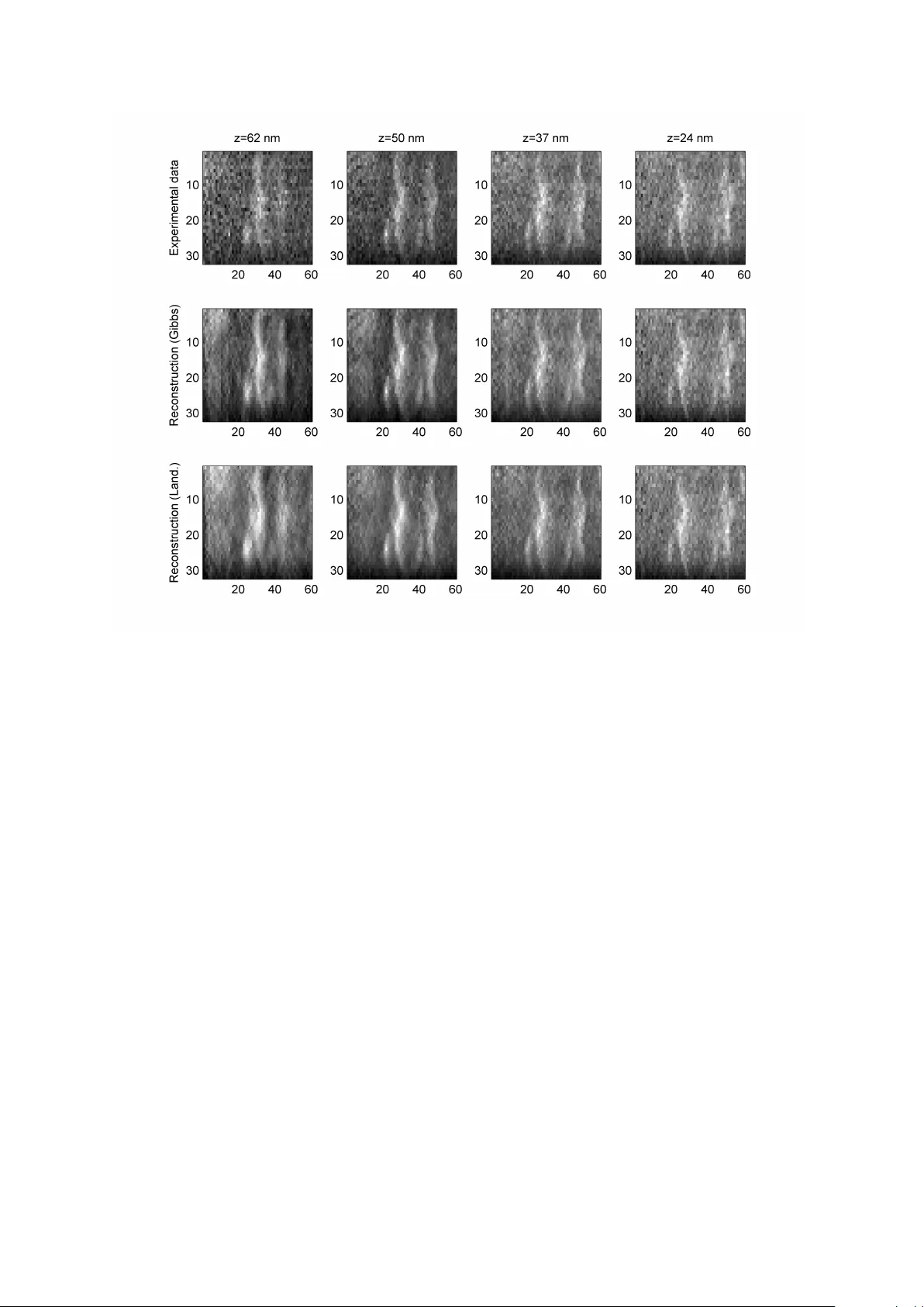
1 Hierarchical Bayesian sparse image reconstruction with application to MRFM Nicolas Dobigeon 1 , 2 , Alfred O. Hero 2 and Jean-Yves T ourneret 1 1 Uni versity of T oulouse, IRIT/INP-ENSEEIHT , 2 rue Camichel, 31071 T oulouse, France. 2 Uni versity of Michigan, Department of EECS, Ann Arbor , MI 48109-2122, USA { Nicolas.Dobigeon, Jean-Yves.Tourneret } @enseeiht.fr, hero@umich.edu Abstract This paper presents a hierarchical Bayesian model to reconstruct sparse images when the observations are obtained from linear transformations and corrupted by an additive white Gaussian noise. Our hierarchical Bayes model is well suited to such naturally sparse image applications as it seamlessly accounts for properties such as sparsity and positivity of the image via appropriate Bayes priors. W e propose a prior that is based on a weighted mixture of a positive exponential distribution and a mass at zero. The prior has hyperparameters that are tuned automatically by marginalization ov er the hierarchical Bayesian model. T o overcome the complexity of the posterior distribution, a Gibbs sampling strategy is proposed. The Gibbs samples can be used to estimate the image to be recovered, e.g. by maximizing the estimated posterior distribution. In our fully Bayesian approach the posteriors of all the parameters are av ailable. Thus our algorithm provides more information than other previously proposed sparse reconstruction methods that only give a point estimate. The performance of the proposed hierarchical Bayesian sparse reconstruction method is illustrated on synthetic data and real data collected from a tobacco virus sample using a prototype MRFM instrument. Index T erms Decon v olution, MRFM imaging, sparse representation, Bayesian inference, MCMC methods. Part of this w ork has been supported by AR O MURI grant No. W911NF-05-1-0403. October 24, 2018 DRAFT 2 I . I N T RO D U C T I O N For se v eral decades, image decon v olution has been of increasing interest [2], [47]. Image decon v olution is a method for reconstructing images from observations provided by optical or other de vices and may include denoising, deblurring or restoration. The applications are numerous including astronomy [49], medical imagery [48], remote sensing [41] and photography [55]. More recently , a ne w imaging technology , called Magnetic Resonance Force Microscopy (MRFM), has been de veloped (see [38] and [29] for revie ws). This non- destructi ve method allows one to improve the detection sensitivity of standard magnetic resonance imaging (MRI) [46]. Three dimensional MRI at 4 nm spatial resolution has recently been achiev ed by the IBM MRFM prototype for imaging the proton density of a tobacco virus [8]. Because of its potential atomic-le vel resolution 1 , the 2 -dimensional or 3 -dimensional images resulting from this technology are naturally sparse in the standard pixel basis. Indeed, as the observed objects are molecules, most of the image is empty space. In this paper , a hierarchical Bayesian model is proposed to perform reconstruction of such images. Sparse signal and image decon v olution has moti v ated research in many scientific applica- tions including: spectral analysis in astronomy [4]; seismic signal analysis in geophysics [7], [45]; and decon v olution of ultrasonic B-scans [39]. W e propose here a hierarchical Bayesian model that is based on selecting an appropriate prior distrib ution for the unknown image and other unkno wn parameters. The image prior is composed of a weighted mixture of a standard exponential distrib ution and a mass at zero. When the non-zero part of this prior is chosen to be a centered normal distrib ution, this prior reduces to a Bernoulli-Gaussian process. This distribution has been widely used in the literature to b uild Bayesian estimators for sparse decon v olution problems (see [5], [16], [24], [28], [33] or more recently [3] and [17]). Ho we ver , choosing a distribution with heavier tail may impro ve the sparsity inducement of the prior . Combining a Laplacian distribution with an atom at zero results in the so-called LAZE prior . This distrib ution has been used in [27] to solve a general denoising problem in a non-Bayesian quasi-maximum likelihood estimation frame work. In [52], [54], this prior has also been used for sparse reconstruction of noisy images, including MRFM. The principal weakness of these previous approaches is the sensitivity to hyperparameters that determine the prior distrib ution, e.g. the LAZE mixture coef ficient and the weighting of the prior vs the 1 Note that the current state of art of the MRFM technology allows one to acquire images with nanoscale resolution. Howe v er , atomic-lev el resolution might be obtained in the future. October 24, 2018 DRAFT 3 likelihood function. The hierarchical Bayesian approach proposed in this paper circumvents these dif ficulties. Specifically , a new prior composed of a mass at zero and a single-sided exponential distribution is introduced, which accounts for positivity and sparsity of the pixels in the image. Conjugate priors on the hyperparameters of the image prior are introduced. It is this step that makes our approach hierarchical Bayesian. The full Bayesian posterior can then be deriv ed from samples generated by Markov chain Monte Carlo (MCMC) methods [44]. The estimation of hyperparameters in v olv ed in the prior distribution described above is the most difficult task and poor estimation leads to instability . Empirical Bayes (EB) and Stein unbiased risk (SURE) solutions were proposed in [52], [54] to deal with this issue. Howe v er , instability was observed especially at higher signal-to-noise ratios (SNR). In the Bayesian estimation framew ork, two approaches are av ailable to estimate these hyperparameters. One approach couples MCMC methods to an e xpectation-maximization (EM) algorithm or to a stochastic EM algorithm [30], [32] to maximize a penalized likelihood function. The second approach defines non-informativ e prior distributions for the hyperparameters; introducing a second lev el of hierarchy into the Bayesian formulation. This latter fully Bayesian approach, adopted in this paper , has been successfully applied to signal segmentation [11], [14], [15] and semi-supervised unmixing of hyperspectral imagery [13]. Only a fe w papers ha ve been published on reconstruction of images from MRFM data [6], [8], [56], [58]. In [21], sev eral techniques based on linear filtering and maximum-likelihood principles were proposed that do not exploit image sparsity . More recently , T ing et al. has introduced sparsity penalized reconstruction methods for MRFM (see [54] or [53]). The reconstruction problem has been formulated as a decomposition into a deconv olution step and a denoising step, yielding an iterati v e thresholding frame work. In [54] the hyperparameters are estimated using penalized log-likelihood criteria including the SURE approach [50]. Despite promising results, especially at lo w SNR, penalized likelihood approaches require iterativ e maximization algorithms that are often slow to con ver ge and can get stuck on local maxima [10]. In contrast to [54], the fully Bayesian approach presented in this paper con v erges quickly and produces estimates of the entire posterior and not just the local maxima. Indeed, the hierarchical Bayesian formulation proposed here generates Bayes-optimal estimates of all image parameters, including the hyperparameters. In this paper, the response of the MRFM imaging device is assumed to be known. While it may be possible to extend our methods to unkno wn point spread functions, e.g., along October 24, 2018 DRAFT 4 the lines of [22], [23], the case of sparse blind decon v olution is outside of the scope of this paper . This paper is or ganized as follows. The decon v olution problem is formulated in Section II. The hierarchical Bayesian model is described in Section III. Section IV presents a Gibbs sampler that allo ws one to generate samples distrib uted according to the posterior of interest. Simulation results, including extensi v e performance comparison, are presented in Section V. In Section VI we apply our hierarchical Bayesian method to reconstruction of a tobacco virus from real MRFM data. Our main conclusions are reported in Section VII. I I . P RO B L E M F O R M U L A T I O N Let X denote a l 1 × . . . × l n unkno wn n -dimensional pixelated image to be recov ered (e.g. n = 2 or n = 3 ). Observ ed are a collection of P projections y = [ y 1 , . . . , y P ] T which are assumed to follow the model: y = T ( κ , X ) + n , (1) where T ( · , · ) stands for a bilinear function, n is a P × 1 dimension noise vector and κ is the kernel that characterizes the response of the imaging device. In the right-hand side of (1), n is an additive Gaussian noise sequence distributed according to n ∼ N ( 0 , σ 2 I P ) , where the v ariance σ 2 is assumed to be unknown. Note that in standard deblurring problems, the function T ( · , · ) represents the standard n - dimensional con volution operator ⊗ . In this case, the image X can be vectorized yielding the unknown image x ∈ R M with M = P = l 1 l 2 . . . l n . W ith this notation, Eq. (1) can be re written: y = Hx + n or Y = κ ⊗ X + N (2) where y (resp. n ) stands for the vectorized version of Y (resp. N ) and H is an P × M matrix that describes con v olution by the point spread function (psf) κ . The problem addressed in the following sections consists of estimating x and σ 2 under sparsity and positivity constraints on x giv en the observations y , the psf κ and the bilinear function 2 T ( · , · ) . 2 In the following, for sake of conciseness, the same notation T ( · , · ) will be adopted for the bilinear operations used on n -dimensional images X and used on M × 1 vectorized images x . October 24, 2018 DRAFT 5 I I I . H I E R A R C H I C A L B A Y E S I A N M O D E L A. Likelihood function The observation model defined in (1) and the Gaussian properties of the noise sequence n yield: f  y | x , σ 2  =  1 2 π σ 2  P 2 exp − k y − T ( κ , x ) k 2 2 σ 2 ! , (3) where k·k denotes the standard ` 2 norm: k x k 2 = x T x . B. P ar ameter prior distributions The unkno wn parameter vector associated with the observation model defined in (1) is θ = { x , σ 2 } . In this section, we introduce prior distrib utions for these tw o parameters; which are assumed to be independent. 1) Image prior: First consider the exponential distribution with shape parameter a > 0 : g a ( x i ) = 1 a exp  − x i a  1 R ∗ + ( x i ) , (4) where 1 E ( x ) is the indicator function defined on E : 1 E ( x ) =    1 , if x ∈ E , 0 , otherwise. (5) Choosing g a ( · ) as prior distributions for x i ( i = 1 , . . . , M ) leads to a maximum a posteriori (MAP) estimator of x that corresponds to a maximum ` 1 -penalized likelihood estimate with a positi vity constraint 3 . Indeed, assuming the component x i ( i = 1 , . . . , P ) a priori independent allo ws one to write the full prior distribution for x = [ x 1 , . . . , x M ] T : g a ( x ) =  1 a  M exp  − k x k 1 a  1 { x  0 } ( x ) , (6) where { x  0 } =  x ∈ R M ; x i > 0 , ∀ i = 1 , . . . , M  and k·k 1 is the standard ` 1 norm k x k 1 = P i | x i | . This estimator has interesting sparseness properties for Bayesian estimation [1] and signal representation [20]. Coupling a standard probability density function (pdf) with an atom at zero is another alternati ve to encourage sparsity . This strategy has for instance been used for located e vent detection [28] such as spike train decon v olution [5], [7]. In order to increase the sparsity of 3 Note that a similar estimator using a Laplacian prior for x i ( i = 1 , . . . , M ) was proposed in [51] for regression problems, referred to as the LASSO estimator, but without positivity constraint. October 24, 2018 DRAFT 6 the prior, we propose to use the follo wing distribution deriv ed from g a ( · ) as prior distribution for x i : f ( x i | w , a ) = (1 − w ) δ ( x i ) + w g a ( x i ) , (7) where δ ( · ) is the Dirac function. This prior is similar to the LAZE distribution (Laplacian pdf and an atom at zero) introduced in [27] and used, for example, in [52], [54] for MRFM. Ho we ver , since g a ( x i ) is zero for x i ≤ 0 , the proposed prior in (7) accounts for the positi vity of the non-zero pixel v alues, a constraint that exists in many imaging modalities such as MRFM. By assuming the components x i to be a priori independent ( i = 1 , . . . , M ), the follo wing prior distribution for x is obtained: f ( x | w , a ) = M Y i =1 [(1 − w ) δ ( x i ) + w g a ( x i )] . (8) Introducing the index subsets I 0 = { i ; x i = 0 } and I 1 = I 0 = { i ; x i 6 = 0 } allows one to re write the previous equation as follows: f ( x | w , a ) = " (1 − w ) n 0 Y i ∈I 0 δ ( x i ) # " w n 1 Y i ∈I 1 g a ( x i ) # , (9) with n  = card {I  } ,  ∈ { 0 , 1 } . Note that n 0 = M − n 1 and n 1 = k x k 0 where k·k 0 is the standard ` 0 norm k x k 0 = # { i ; x i 6 = 0 } . 2) Noise variance prior: A conjugate in v erse-Gamma distrib ution with parameters ν 2 and γ 2 is chosen as prior distribution for the noise variance [43, Appendix A]: σ 2 | ν, γ ∼ I G  ν 2 , γ 2  . (10) In the follo wing, the shape parameter ν will be fix ed to ν = 2 and the scale parameter γ will be estimated as an hyperparameter (see [13], [14], [40]). Note that choosing the in v erse-Gamma distribution I G  ν 2 , γ 2  as a prior for σ 2 is equi v alent to choosing a Gamma distribution G  ν 2 , γ 2  as a prior for 1 /σ 2 . C. Hyperparameter priors The hyperparameter vector associated with the aforementioned prior distributions is Φ = { a, γ , w } . Obviously , the accurac y of the proposed Bayesian model depends on the values of these hyperparameters. Sometimes prior knowledge may be av ailable, e.g., the mean number of non-zero pixels in the image. In this case these parameters can be tuned manually to their true values. Ho we ver , in many practical situations such prior information is not av ailable and these hyperparameters must be estimated directly from the data. Priors for these hyperparameters, sometimes referred to as “hyperpriors” are giv en below . October 24, 2018 DRAFT 7 1) Hyperparameter a : A conjugate in v erse-Gamma distribution is assumed for the scale parameter a of the distribution g a ( · ) of non-zero pixel intensities: a | α ∼ I G ( α 0 , α 1 ) , (11) with α = [ α 0 , α 1 ] T . Similarly to [19], the fixed hyperparameters α 0 and α 1 hav e been chosen to obtain a v ague prior: α 0 = α 1 = 10 − 10 . 2) Hyperparameter γ : A non informati ve Jef fre ys’ prior [25], [26] is assumed for the scale parameter of the in verse Gamma prior density on the noise variance σ 2 : f ( γ ) ∝ 1 γ 1 R + ( γ ) . (12) The combination of the priors (10) and (12) yields the non-informati ve Jeffre ys’ prior on σ 2 . Note that there is no difference between choosing a non-informati ve Jeffre y’ s prior for σ 2 and the proper hierarchical prior defined by (10) and (12). Indeed, integrating o ver the hyperparameter γ in the joint f ( σ 2 , γ ) distribution yields: f  σ 2  = Z f  σ 2 | γ  f ( γ ) dγ ∝  1 σ 2  2 Z exp  − γ 2 σ 2  dγ ∝ 1 σ 2 . (13) Ho we ver , in more complex noise models the hierarchical priors f ( σ 2 | γ ) and f ( γ ) are not equi v alent to such a simple prior on σ 2 . For example, as in [12], this pair of hierarchical priors is easily generalizable to conditionally Gaussian noise with spatial correlation and spatially varying signal-to-noise ratio. 3) Hyperparameter w : A uniform distribution on the simplex [0 , 1] has been chosen as prior distribution for the mean proportion of non-zero pixels: w ∼ U ([0 , 1]) . (14) This is the least informati ve prior on the image sparsity factor . Assuming that the individual hyperparameters are statistically independent the full hyperparameter prior distribution for Φ can be expressed as: f ( Φ | α ) = f ( w ) f ( γ ) f ( a ) ∝ 1 γ a α 0 +1 exp  − α 1 a  × 1 [0 , 1] ( w ) 1 R + ( a ) 1 R + ( γ ) , (15) October 24, 2018 DRAFT 8 Fig. 1. D A G for the parameter priors and hyperpriors (the fixed non-random hyperparameters appear in dashed boxes). D. P osterior distribution The posterior distribution of { θ , Φ } can be computed as follows: f ( θ , Φ | y , α ) ∝ f ( y | θ ) f ( θ | Φ ) f ( Φ | α ) , (16) with f ( θ | Φ ) = f ( x | a, w ) f  σ 2 | γ  , (17) where f ( y | θ ) and f ( Φ | α ) hav e been defined in (3) and (15). This hierarchical structure, represented on the directed acyclic graph (D A G) in Fig. 1, allows one to integrate out the parameter σ 2 and the hyperparameter vector Φ in (16) to obtain the posterior of the image gi ven the measured data and the parameters x : f ( x | y , α ) ∝ B (1 + n 1 , 1 + n 0 ) k y − T ( κ , x ) k P × Γ ( n 1 + α 0 ) [ k x k 1 + α 1 ] n 1 + α 0 1 { x  0 } ( x ) . (18) In (18), as defined in paragraph III-B.1, n 1 = k x k 0 , n 0 = M − k x k 0 and B ( · , · ) stands for the Beta function B ( u, v ) = Γ ( u ) Γ ( v ) / Γ ( u + v ) , where Γ( · ) denotes the Gamma function. The next section presents an appropriate Gibbs sampling strategy [44, Chap. 10] that allows one to generate an image sample distributed according to the posterior distribution f ( x | y , α ) . October 24, 2018 DRAFT 9 I V . A G I B B S S A M P L I N G S T R A T E G Y F O R S P A R S E I M A G E R E C O N S T R U C T I O N In this section, we describe the Gibbs sampling strategy for generating samples  x ( t )  t =1 ,... distributed according to the posterior distribution in (18). As simulating directly according to (18) is difficult, it is much more con v enient to generate samples distributed according to the joint posterior f ( x , σ 2 , a, w | y , α ) . This Gibbs sampler produces sequences  x ( t )  t =1 ,... ,  σ 2( t )  t =1 ,... ,  a ( t )  t =1 ,... ,  w ( t )  t =1 ,... which are Marko v chains with stationary distributions f ( x | y , α ) , f ( σ 2 | y , α ) , f ( a | y , α ) and f ( w | y , α ) , respectiv ely [44, p. 345]. Then, the MAP estimator of the unknown image x will be computed by retaining among X =  x ( t )  t =1 ,... the generated sample that maximizes the posterior distribution in (18) [35, p. 165]: ˆ x MAP = argmax x ∈ R M + f ( x | y ) ≈ argmax x ∈X f ( x | y ) . (19) The main steps of this algorithm are gi v en in subsections IV -A and IV -D (see also Algorithm 1 belo w). A L G O R I T H M 1 : Gibbs sampling algorithm f or sparse image reconstruction • Initialization: – Sample parameter x (0) from the pdf in (9), – Sample parameter e σ 2(0) from the pdf in (10), – Set t ← 1 , • Iterations: for t = 1 , 2 , . . . , do 1. Sample hyperparameter w ( t ) from the pdf in (21), 2. Sample hyperparameter a ( t ) from the pdf in (22), 3. For i = 1 , . . . , M , sample parameter x ( t ) i from the pdf in (23), 4. Sample parameter e σ 2( t ) from the pdf in (26), 5. Set t ← t + 1 . October 24, 2018 DRAFT 10 A. Generation of samples accor ding to f ( w | x ) Using (9), the follo wing result can be obtained: f ( w | x ) ∝ (1 − w ) n 0 w n 1 , (20) where n 0 and n 1 hav e been defined in paragraph III-B.1. Therefore, samples from f ( w | x ) can be generated by simulating from an image dependent Beta distribution: w | x ∼ B e (1 + n 1 , 1 + n 0 ) . (21) B. Generation of samples accor ding to f ( a | x , α ) The form of the joint posterior distribution (16) implies that samples of a can be generated by simulating from an image dependent in v erse-Gamma distribution: a | x , α ∼ I G ( k x k 0 + α 0 , k x k 1 + α 1 ) . (22) C. Generation of samples accor ding to f ( x | w , a, σ 2 , y ) The LAZE-type prior (7) chosen for x i ( i = 1 , . . . , M ) yields a posterior distribution of x that is not closed form. Howe v er , one can easily deriv e the posterior distribution of each pixel intensity x i ( i = 1 , . . . , M ) conditioned on the intensities of the rest of the image. Indeed straightforward computations (Appendix I) yield: f  x i | w , a, σ 2 , x − i , y  ∝ (1 − w i ) δ ( x i ) + w i φ +  x i | µ i , η 2 i  , (23) where x − i stands for the vector x whose i th component has been removed and µ i and η 2 i are gi ven in Appendix I. In (23), φ + ( · , m, s 2 ) stands for the pdf of the truncated Gaussian distribution defined on R ∗ + with hidden mean and variance parameters equal to m and s 2 , respecti vely: φ +  x, m, s 2  = 1 C ( m, s 2 ) exp " − ( x − m ) 2 2 s 2 # 1 R ∗ + ( x ) , (24) with C  m, s 2  = r π s 2 2  1 + erf  m √ 2 s 2  . (25) The form in (23) specifies x i | w , a, σ 2 , x − i , y as a Bernoulli-truncated Gaussian variable with parameter ( w i , µ i , η 2 i ) . Appendix III presents an algorithm that can be used to generate samples from this distrib ution. This algorithm generates samples distrib uted according to f ( x | w , σ 2 , a, y ) by successi v ely updating the coordinates of x using a sequence of M Gibbs mov es (requiring generation of Bernoulli-truncated Gaussian v ariables). October 24, 2018 DRAFT 11 D. Generation of samples accor ding to f ( σ 2 | x , y ) Samples are generated in the following way: σ 2 | x , y ∼ I G P 2 , k y − T ( κ , x ) k 2 2 ! . (26) V . S I M U L A T I O N O N S Y N T H E T I C I M A G E S T ABLE I P A R A M E T E R S U S E D T O C O M P U T E T H E M R F M P S F . Parameter V alue Description Name Amplitude of external magnetic field B ext 9 . 4 × 10 3 G V alue of B mag in the resonant slice B res 1 . 0 × 10 4 G Radius of tip R 0 4 . 0 nm Distance from tip to sample d 6 . 0 nm Cantilev er tip moment m 4 . 6 × 10 5 emu Peak cantilev er oscillation x pk 0 . 8 nm Maximum magnetic field gradient G max 125 Fig. 2. Left: Psf of the MRFM tip. Right: unknown sparse image to be estimated. October 24, 2018 DRAFT 12 A. Reconstruction of 2-dimensional image In this subsection, a 32 × 32 synthetic image, depicted in Fig. 2 (right panel), is simulated using the prior in (9) with parameters a = 1 and w = 0 . 02 . In Figs. 2 and 3, white pixels stands for zero intensity v alues. A general analytical deri v ation of the psf of the MRFM tip has been gi ven in [34] and with further explanation in [54]. Follo wing this model, we defined a 10 × 10 2 -dimensional con volution k ernel, the psf represented in Fig. 2 (left panel), that corresponds to the physical parameters shown in T able I. The associated psf matrix H introduced in (2) is of size 1024 × 1024 . The observed measurements y , which are of size P = 1024 and depicted in Fig. 3 (top panel), are corrupted by an additi ve Gaussian noise with two different variances σ 2 = 1 . 2 × 10 − 1 and σ 2 = 1 . 6 × 10 − 3 , corresponding to signal-to-noise ratios SNR = 2 dB and SNR = 20 dB, respectiv ely . 1) Simulation results: The observations are processed by the proposed algorithm using N MC = 2000 iterations of the Gibbs sampler with N bi = 300 burn-in iterations. The compu- tation time for completing 100 iterations of the proposed algorithm is 80 s for an unoptimized MA TLAB 2007b 32bit implementation on a 2.2GHz Intel Core 2, while 100 iterations of the Landweber and empirical Bayesian algorithms require 0 . 15 s and 2 s, respectiv ely . The MAP image reconstruction computed using (19) is depicted in Fig. 3 (bottom panel) for the two le vels of noise considered. Observe that the estimated image is very similar to the actual image, Fig. 2 (right panel), ev en at low SNR. Moreov er , as the proposed algorithm generates samples distributed according to the poste- rior distribution in (18), these samples can be used to compute the posterior distributions of each parameter . For illustration, the posterior distributions of the hyperparameters a and w , as well as the noise variance σ 2 , are sho wn in Fig. 4, 5 and 6. These estimated distributions are in good agreement with the ground truth v alues of these parameters, randomly dra wn from the prior distribution. In many applications, a measure of confidence that a gi v en pixel or pixel region is non-zero is of interest. Our Bayesian approach can easily generate such measures of confidence in the form of posterior probabilities of the specified ev ent, sometimes known as the Bayesian p- v alue. F ollo wing the strategy detailed in Appendix III, the proposed Gibbs sampler generates a collection of samples  x ( t )  t =1 ,...,N MC , distrib uted according the posterior Bernoulli-truncated Gaussian distrib ution in (23). This sampling requires the generation of indicator v ariables z i ( i = 1 , . . . , n ) that reflect the presence or the absence of non-zero pixel values. It is the October 24, 2018 DRAFT 13 Fig. 3. T op, left (resp. right): noisy observations for SNR = 2 dB (resp. 20 dB). Bottom, left (resp. right): reconstructed image for SNR = 2 dB (resp. 20 dB). Fig. 4. Posterior distribution of hyperparameter a (left: SNR = 2 dB, right: SNR = 20 dB). October 24, 2018 DRAFT 14 Fig. 5. Posterior distribution of hyperparameter w (left: SNR = 2 dB, right: SNR = 20 dB). Fig. 6. Posterior distribution of hyperparameter σ 2 (left: SNR = 2 dB, right: SNR = 20 dB). indicator variable z i that x i > 0 that provides information about non-zero pixels in the image. Using the equi v alences { z i = 0 } ⇔ { x i = 0 } and { z i = 1 } ⇔ { x i > 0 } , the posterior probability P [ x i > 0 | y , α ] can be easily obtained by a veraging ov er the Gibbs samples of the binary variables n z ( t ) i o t = N bi +1 ,...,N MC . T o illustrate, these probabilities are depicted in Fig. 7. In addition, these Gibbs samples can be used to compute the probability of having non-zero pixels in a giv en area of the image. The estimated posterior probability for the ev ent that a non-zero pixel is present inside the small red rectangle in the figure is equal to 45% for the case of SNR = 2 dB. Con v ersely , the posterior probability of having a non-zero pixel in the green box is 5% . For SNR = 20 dB the MAP algorithm correctly detects up the presence of a October 24, 2018 DRAFT 15 pixel in this region. On the other hand, ev en though at SNR = 2 dB the MAP reconstruction has not detected this pixel, we can be 45% confident of the presence of such a pixel in the red rectangular region on the left panel of Fig. (7). Fig. 7. Posterior probabilities of ha ving non-zero pixels (left: SNR = 2 dB, right: SNR = 20 dB). The probability of having at least one non-zero pixel in the red (resp. green) box-delimited area is 45% (resp. 5% ). The posterior distrib utions of four dif ferent pixels are depicted in Fig. 8. These posteriors are consistent with the actual values of these pixels that are represented as dotted red lines in these figures. In particular , in all cases the actual values all lie within the 75% central quantile of the posterior distribution. 2) Comparison of r econstruction performances: Here we compare our proposed hierar- chical Bayesian method to the sparse reconstruction methods of [52], [54]. The techniques proposed in [52], [54] are based on penalized likelihood EM algorithms that perform empirical estimation of the unknown hyperparameters. Therein, two empirical Bayesian estimators, denoted Emp-MAP-Lap and Emp-MAP-LAZE, based on a Laplacian or a LAZE prior respecti vely , were proposed. W e also compare to the standard Landweber algorithm [31] that has been previously used to perform MRFM image reconstruction [8], [57]. These are compared to our hierarchical Bayesian MAP reconstruction algorithm, giv en in (19), and also to a minimum mean square error (MMSE) reconstruction algorithm extracted from the estimated full Bayes posterior (18). The MMSE estimator of the image x is obtained by October 24, 2018 DRAFT 16 Fig. 8. Posterior distributions of the non-zero values of x for 4 dif ferent pixel locations and for SNR = 20 dB (actual pixel intensity values are depicted with dotted red lines). empirical averaging ov er the last N r = 1700 samples of the Gibbs sampler according to: ˆ x MMSE = E [ x | y ] ≈ 1 N r N r X t =1 x ( N bi + t ) . (27) As in [54] we compare the various reconstruction algorithms with respect to sev eral performance criteria. Let e = x − ˆ x denote the reconstruction error when ˆ x is the estimator of the image x to be recov ered. These criteria are: the ` 0 , ` 1 and ` 2 -norms of e , which measures the accuracy of the reconstruction, and the ` 0 -norm of the estimator ˆ x , which measures its sparsity . As pointed out in [54], a human observer can usually not visually detect the presence of non-zero intensities if they are below a small threshold. Thus, a less strict measure 4 of 4 The introduced measure of sparsity is denoted k·k δ . This is an abuse of notation since it is not a norm. October 24, 2018 DRAFT 17 sparsity than the ` 0 -norm, which is denoted k·k δ , is the number of reconstructed image pixels that are less than a giv en threshold δ : k ˆ x k δ = M X i =1 1 ˆ x i <δ ( ˆ x i ) , k e k δ = M X i =1 1 e i <δ ( e i ) . (28) It what follows, δ has been chosen as δ = 10 − 2 k x k ∞ . T o summarize, the following criteria hav e been computed for the image in paragraph V -A.1 for two levels of SNR: k e k 0 , k e k δ , k e k 1 , k e k 2 , k ˆ x k 0 and k ˆ x k δ . T able II sho ws the six performance measures for the five dif ferent algorithms studied. The proposed Bayesian methods (labeled “proposed MMSE” and “proposed MAP” in the table) outperform the other reconstruction algorithms in terms of ` 1 or ` 2 -norms. Note that the MMSE estimation of the unkno wn image is a non sparse estimator in the ` 0 -norm sense. This is due to the very small but non-zero posterior probability of non-zero value at many pixels. The sparsity measure k·k δ indicates that most of the pixels are in fact very close to zero. The MAP reconstruction method seems to achiev e the best balance between the sparsity of the solution and the minimization of the reconstruction error . Of course, by its very construction, the MMSE reconstruction will always hav e lower mean square error . B. Reconstruction of undersampled 3-dimensional images As discussed below in Section VI, the prototype IBM MRFM instrument [8] collects data projections as irregularly spaced, or undersampled, spatial samples. In this subsection, we indicate ho w the image reconstruction algorithm can be adapted to this undersampled scenario in 3D. W e illustrate by a concrete example. First, a 24 × 24 × 6 image is generated such that 4 pixels ha ve non-zero v alues in each z slice. The resulting data is depicted in Fig. 9 (top) and Fig. 10 (left). This image to be reco vered is assumed to be con v olved with a 5 × 5 × 3 k ernel that is represented in Fig. 10 (right). The resulting con v olved image is depicted in Fig. 11 (left). Howe v er , the actual observed image is an undersampled version of this image. More precisely , the sampling rates are assumed to be d x = 2 , d y = 3 , d z = 1 , respectiv ely , in the 3 dimensions. Consequently the observ ed 3 D image, sho wn in Fig. 11, is of size 12 × 8 × 6 . Finally , an i.i.d. Gaussian noise with σ = 0 . 02 is added following the model in (1). Note that under these assumptions, the application T ( · , · ) can be split into two standard operations October 24, 2018 DRAFT 18 T ABLE II R E C O N S T RU C T I O N P E R F O R M A N C E S F O R D I FF E R E N T S PA R S E I M AG E R E C O N S T R U C T I O N A L G O R I T H M S . Method Error criterion k e k 0 k e k δ k e k 1 k e k 2 k ˆ x k 0 k ˆ x k δ SNR = 2 dB Landweber 1024 990 339.76 13.32 1024 990 Emp-MAP-Lap 18 17 14.13 4.40 0 0 Emp-MAP-LAZE 60 58 9.49 1.44 55 55 Proposed MMSE 1001 30 3.84 0.72 1001 27 Proposed MAP 19 16 2.38 0.81 13 13 SNR = 20 dB Landweber 1024 931 168.85 6.67 1024 931 Emp-MAP-Lap 33 18 1.27 0.31 28 23 Emp-MAP-LAZE 144 19 1.68 0.22 144 27 Proposed MMSE 541 5 0.36 0.11 541 16 Proposed MAP 19 7 0.39 0.13 16 16 follo wing the composition: T ( κ , X ) = g d x ,d y ,d z ( κ ⊗ X ) , (29) where g d x ,d y ,d z ( · ) stands for the undersampling function. The proposed hierarchical Bayesian algorithm is used to perform the sparse reconstruction with undersampled data. The number of Monte Carlo runs was fixed to N MC = 2000 with N bi = 300 burn-in iterations. Figure 9 shows the result of applying the proposed MAP estimator to the estimated posterior . V I . A P P L I C AT I O N O N R E A L M R F M I M AG E S Here we illustrate the hierarchical Bayesian MAP reconstruction algorithm for real three dimensional MRFM data. The data is a set of MRFM projections of a sample of tobacco virus. Comprehensiv e details of both the experiment and the MRFM data acquisition protocol are giv en in [8] and the supplementary materials [9]. The observ ed sample consists of a October 24, 2018 DRAFT 19 Fig. 9. T op: slices of the sparse image to be recovered. Bottom: slices of the estimated sparse image. Fig. 10. Left: 24 × 24 × 6 unknown image to be recovered. Right: 5 × 5 × 3 kernel modeling the psf. collection of T obacco mosaic virus particles that constitute a whole viral segment in addition to viral fragments. The projections are computed from the measured proton distribution and October 24, 2018 DRAFT 20 Fig. 11. Left: 24 × 24 × 6 regularly sampled con volv ed image. Left: 12 × 8 × 6 undersampled observed image. the 3 -dimensional psf following the protocol described in [8] and [9]. The resulting scan data are depicted in Figure 12 (top) for four different distances between the MRFM tip and the sample: d = 24 nm, d = 37 nm, d = 50 nm and d = 62 nm. Each of these x-y slices is of size 60 × 32 pixels. These experimental data are undersampled, i.e. the spatial resolution of the MRFM tip, and therefore the psf function, is finer than the resolution of the observed slices. Consequently , these data hav e been decon volv ed taking into account the ov ersampling rates defined by d x = 3 , d y = 2 and d z = 3 in the three directions. The MAP estimate of the unknown image is computed from N MC = 1000 Gibbs samples of the proposed Bayesian algorithm initialized with the output of a single Landweber iteration. Se v eral more iterations of the Landweber algorithm would produce the reconstructions reported in [8]. Three horizontal slices of the October 24, 2018 DRAFT 21 Fig. 12. T op: experimental scan data where black (resp. white) pixel represents low (resp. high) density of spin (as in [8]). Middle: scan data reconstructed from the proposed hierarchical Bayesian algorithm. Bottom: scan data reconstructed from the Landweber algorithm. estimated image 5 are depicted in Figure 13. A 3 -dimensional vie w of the estimated profile of the virus fragments is sho wn in Figure 14. The MMSE estimates of the parameters introduced in Section III are ˆ σ 2 MMSE = 0 . 10 , ˆ a MMSE = 1 . 9 × 10 − 12 and ˆ w MMSE = 1 . 4 × 10 − 2 . The image reconstructions produced by the Landweber and Bayesian MAP algorithms are sho wn in Fig. 12. By forward projecting the estimated virus image through the point spread function one can visually e v aluate the goodness of fit of the reconstruction to the ra w measured data. This is depicted in Fig. 12. These figures are clearly in good agreement with the observed data (top). T o ev aluate the con v ergence speed, the reconstruction error is represented in Figure 15 5 Note that most part of the estimated 3 dimensional image is empty space due to the very localized proton spin centers in the image. October 24, 2018 DRAFT 22 Fig. 13. Three horizontal slices of the estimated image. Fig. 14. 3 -dimensional view of the estimated profile of the T obacco virus fragments. as a function of the iterations for the proposed Bayesian and the Landweber algorithms. This sho ws that the con ver gence rate of our algorithm is significantly better than the Landweber October 24, 2018 DRAFT 23 algorithm. Fig. 15. Error of the reconstructions as functions of the iteration number for the proposed algorithm (continuous blue line) and Landweber algorithm (dotted red line). V I I . C O N C L U S I O N S This paper presented a hierarchical Bayesian algorithm for decon v olving sparse positiv e images corrupted by additive Gaussian noise. A Bernoulli-truncated exponential distribution was proposed as a prior for the sparse image to be reco vered. The unkno wn hyperparameters of the model were integrated out of the posterior distribution of the image, producing a full posterior distribution that can be used for estimation of the pix el v alues by extracting the mode (MAP) or the first moment (MMSE). An ef ficient Gibbs sampler was used to generate approximations to these estimates. The deri v ed Bayesian estimators significantly outperformed sev eral previously proposed sparse reconstruction algorithms. Our approach was implemented on real MRFM data to reconstruct a 3 D image of a tobacco virus. Future work will include extension of the proposed method to other sparse bases, inclusion of uncertain point spread functions, and in vestigation of molecular priors. Future in v estigations might also include a comparison between the proposed MCMC approach and v ariational Bayes approaches. A P P E N D I X I D E R I V A T I O N O F T H E C O N D I T I O N A L October 24, 2018 DRAFT 24 P O S T E R I O R D I S T R I B U T I O N f ( x i | w , a, σ 2 , x − i , y ) The posterior distrib ution of each component x i ( i = 1 , . . . , M ) conditionally upon the others is linked to the likelihood function (3) and the prior distribution (7) via the Bayes’ formula: f  x i | w , a, σ 2 , x − i , y  ∝ f  y | x , σ 2  f ( x i | w , a ) . (30) This distrib ution can be easily deriv ed by decomposing x on the standard orthonormal basis B = { u 1 , . . . , u M } , (31) where u i is the i th column of the M × M identity matrix. Indeed, let decompose x as follo ws: x = ˜ x i + x i u i , (32) where ˜ x i is the v ector x whose i th element has been replaced by 0 . Then the linear property of the operator T ( κ , · ) allo ws one to state: T ( κ , x ) = T ( κ , ˜ x i ) + x i T ( κ , u i ) . (33) Consequently , (30) can be rewritten f  x i | w , a, σ 2 , x − i , y  ∝ exp − k e i − x i h i k 2 2 σ 2 ! × h (1 − w ) δ ( x i ) + w a exp  − x i a  1 R ∗ + ( x i ) i , (34) where 6    e i = y − T ( κ , ˜ x i ) , h i = T ( κ , u i ) . (35) An efficient way to compute e i within the Gibbs sampler scheme is reported in Appendix II. Then, straightforward computations similar to those in [7] and [37, Annex B] yield to the follo wing distribution: f  x i | w , a, σ 2 , x − i , y  ∝ (1 − w i ) δ ( x i ) + w i φ +  x i | µ i , η 2 i  , (36) with          η 2 i = σ 2 k h i k 2 , µ i = η 2 i  h T i e i σ 2 − 1 a  , (37) 6 It can be noticed that, for deblurring applications, h i is also the i th column of the matrix H introduced in (2). October 24, 2018 DRAFT 25 and        u i = w a C  µ i , η 2 i  exp  µ 2 i 2 η 2 i  , w i = u i u i + (1 − w ) . (38) The distribution in (36) is a Bernoulli-truncated Gaussian distribution with hidden mean µ i and hidden variance η 2 i . A P P E N D I X I I F A S T R E C U R S I V E C O M P U TA T I O N S F O R S I M U L AT I N G AC C O R D I N G T O f ( x | w , a, σ 2 , y ) In the Gibbs sampling strategy presented in Section IV, the main computationally expensi ve task is the generation of samples distributed according to f ( x i | w , a, σ 2 , x − i , y ) . Indeed, the e v aluation of the hidden mean and hidden v ariance in (37) of the Bernoulli-truncated Gaussian distribution may be costly , especially when the bilinear application T ( · , · ) is not easily computable. In this appendix, an appropriate recursi ve strategy is proposed to accelerate the Gibbs sampling by ef ficiently updating the coordinate i of the vector x at iteration t of the Gibbs sampler . Let x ( t,i − 1) denote the current Monte Carlo state of the unknown v ectorized image x ( i = 1 , . . . , M ): x ( t,i − 1) = h x ( t ) 1 , . . . , x ( t ) i − 1 , x ( t − 1) i , x ( t − 1) i +1 , . . . , x ( t − 1) M i T . (39) with, by definition, x ( t, 0) = x ( t − 1 ,M ) . Updating x ( t,i − 1) consists of drawing x ( t ) i according to the Bernoulli-truncated Gaussian distribution f  x i    w , a, σ 2 , x ( t,i − 1) − i , y  in (23) with: x ( t,i − 1) − i = h x ( t ) 1 , . . . , x ( t ) i − 1 , x ( t − 1) i +1 , . . . , x ( t − 1) M i T . (40) The proposed strategy to simulate efficiently according to (23) is based on the follo wing property . Pr operty : Gi ven the quantity T  κ , x (0)  and the vectors { h i } i =1 ,...,M , simulating according to f  x i    w , a, σ 2 , x ( t,i ) − i , y  can be performed without e v aluating the bilinear function T ( · , · ) . Pr oof : Simulating according to (23) mainly requires to compute the vector e i introduced by (35): e i = y − T  κ , ˜ x ( t,i − 1) i  , (41) October 24, 2018 DRAFT 26 with ˜ x ( t,i − 1) i = h x ( t ) 1 , . . . , x ( t ) i − 1 , 0 , x ( t − 1) i +1 , . . . , x ( t − 1) M i T . (42) Moreov er , by using the decomposition in (32) and by exploiting the linear property of T ( κ , · ) , the vector T  κ , ˜ x ( t,i − 1) i  in the right-hand side of (41) can be rewritten as: T  κ , ˜ x ( t,i − 1) i  = T  κ , x ( t,i − 1)  − x ( t − 1) i h i , (43) where h i has been introduced in (35). Consequently , to prove the property , we hav e to demonstrate that the v ector series  T  κ , x ( t,k )  k =1 ,...,M can be computed recursi v ely without using T ( · , · ) . Assume that T  κ , x ( t,i − 1)  is av ailable at this stage of the Gibbs sampling and that x ( t ) i has been drawn. The ne w Monte Carlo state is then: x ( t,i ) = h x ( t ) 1 , . . . , x ( t ) i − 1 , x ( t ) i , x ( t − 1) i +1 , . . . , x ( t − 1) M i T . (44) Similarly to (43), the vector T  κ , x ( t,i )  can be decomposed as follows: T  κ , x ( t,i )  = T  κ , ˜ x ( t,i − 1) i  + x ( t ) i h i . (45) Therefore, combining (43) and (45) allow one to state: T  κ , x ( t,i )  = T  κ , x ( t,i − 1)  +  x ( t ) i − x ( t − 1) i  h i .  The bilinear function T ( · , · ) only needs to be used at the very beginning of the Gibbs sam- pling algorithm to e v aluate T  κ , x (0)  and the vectors { h i } i =1 ,...,M . The resulting simulation scheme corresponding to step 3 of Algorithm 1 is shown in Algorithm 2. A P P E N D I X I I I S I M U L AT I O N AC C O R D I N G T O A B E R N O U L L I - T R U N C A T E D G AU S S I A N D I S T R I B U T I O N This appendix describes ho w we generate random variables distributed according to a Bernoulli-truncated Gaussian distribution with parameters ( w i , µ i , η 2 i ) whose pdf is: f  x i | w i , µ i , η 2 i  = (1 − w i ) δ ( x i ) + w i C ( µ i , η 2 i ) exp " − ( x i − µ i ) 2 2 η 2 i # 1 R ∗ + ( x i ) October 24, 2018 DRAFT 27 A L G O R I T H M 2 : Efficient simulation according to f  x   w , a, σ 2 , y  For i = 1 , . . . , M , update the i th coordinate of the vector x ( t,i − 1) = h x ( t ) 1 , . . . , x ( t ) i − 1 , x ( t − 1) i , x ( t − 1) i +1 , . . . , x ( t − 1) M i T via the follo wing steps: 1. compute k h i k 2 , 2. set T  κ , ˜ x ( t,i − 1) i  = T  κ , x ( t,i − 1)  − x ( t − 1) i h i , 3. set e i = x − T  κ , ˜ x ( t,i − 1) i  , 4. compute µ i , η 2 i and w i as defined in (37) and (38), 5. draw x ( t ) i according to (23), 6. set x ( t,i ) = h x ( t ) 1 , . . . , x ( t ) i − 1 , x ( t ) i , x ( t − 1) i +1 , . . . , x ( t − 1) M i T , 7. set T  κ , x ( t,i )  = T  κ , ˜ x ( t,i − 1) i  + x ( t ) i h i . A L G O R I T H M 3 : Simulation according to a Bernoulli-truncated Gaussian distrib ution 1. generate z i according to z i ∼ B er ( w i ) , 2. set    x i = 0 , if z i = 0 ; x i ∼ N +  µ i , η 2 i  , if z i = 1 . where C ( µ i , η 2 i ) has been defined in (25). Monte Carlo draws from this density can be obtained by using an auxiliary binary v ariable z i follo wing the strategy shown in Algorithm 3. This indicator variable takes the value 0 (resp. 1 ) if the pixel x i is zero (resp. non-zero). In Algorithm 3, B er ( · ) and N + ( · , · ) denote the Bernoulli and the positiv e truncated Gaussian distributions respecti vely . In step 2 , samples distributed according to the truncated Gaussian distribution can be generated by using an appropriate accept-reject procedure with instrumental distributions [18], [36], [42]. October 24, 2018 DRAFT 28 A C K N O W L E D G E M E N T S The authors would like to thank Michael T ing (Seagate T echnology) for providing the code to generate point spread functions of MRFM tip and Hichem Snoussi (Univ ersity of T echnology of T royes) for interesting suggestions regarding this work. The authors are also very grateful to Dr . Daniel Rugar who provided the real data used in Section VI as well as a valuable feedback on this paper . R E F E R E N C E S [1] S. Alliney and S. A. Ruzinsky , “ An algorithm for the minimization of mixed l1 and l2 norms with application to Bayesian estimation, ” IEEE T rans. Signal Pr ocessing , vol. 42, no. 3, pp. 618–627, March 1994. [2] H. Andrews and B. Hunt, Digital Image Restoration . Englew ood Cliffs, NJ: Prentice-Hall, 1977. [3] S. Bourguignon and H. Carfantan, “Bernoulli-Gaussian spectral analysis of unevenly spaced astrophysical data, ” in Pr oc. IEEE W orkshop on Stat. Signal Processing (SSP) , Bordeaux, France, July 2005, pp. 811–816. [4] S. Bour guignon, H. Carfantan, and J. Idier , “ A sparsity-based method for the estimation of spectral lines from irre gularly sampled data, ” IEEE J . Sel. T opics Signal Pr ocessing , vol. 1, no. 4, pp. 575–585, Dec. 2007. [5] F . Champagnat, Y . Goussard, and J. Idier , “Unsupervised deconv olution of sparse spike trains using stochastic approximation, ” IEEE Tr ans. Signal Pr ocessing , vol. 44, no. 12, pp. 2988–2998, Dec. 1996. [6] S. Chao, W . M. Dougherty , J. L. Garbini, and J. A. Sidles, “Nanometer-scale magnetic resonance imaging, ” Revie w Sci. Instrum. , vol. 75, no. 5, pp. 1175–1181, April 2004. [7] Q. Cheng, R. Chen, and T .-H. Li, “Simultaneous wav elet estimation and deconv olution of reflection seismic signals, ” IEEE T r ans. Geosci. and Remote Sensing , v ol. 34, no. 2, pp. 377–384, March 1996. [8] C. L. Degen, M. Poggio, H. J. Mamin, C. T . Rettner, and D. Rugar, “Nanoscale magnetic resonance imaging, ” Pr oc. Nat. Academy of Science , vol. 106, no. 5, pp. 1313–1317, Feb. 2009. [9] ——, “Nanoscale magnetic resonance imaging. Supporting information, ” Pr oc. Nat. Academy of Science , vol. 106, no. 5, Feb . 2009. [Online]. A v ailable: www .pnas.org/cgi/content/full/0812068106/DCSupplemental [10] J. Diebolt and E. H. S. Ip., “Stochastic EM: method and application, ” in Markov Chain Monte Carlo in Practice , W . R. Gilks, S. Richardson, and D. J. Spiegelhalter , Eds. London: Chapman & Hall, 1996, pp. 259–273. [11] N. Dobigeon and J.-Y . T ourneret, “Joint se gmentation of wind speed and direction using a hierarchical model, ” Comput. Stat. & Data Analysis , vol. 51, no. 12, pp. 5603–5621, Aug. 2007. [12] ——, “Bayesian sampling of structured noise cov ariance matrix for hyperspectral imagery , ” Univ ersity of T oulouse, T ech. Rep., Dec. 2008. [Online]. A v ailable: http://dobigeon.perso.enseeiht.fr/publis.html [13] N. Dobigeon, J.-Y . T ourneret, and C.-I Chang, “Semi-supervised linear spectral unmixing using a hierarchical Bayesian model for hyperspectral imagery , ” IEEE T r ans. Signal Pr ocessing , vol. 56, no. 7, pp. 2684–2695, July 2008. [14] N. Dobigeon, J.-Y . T ourneret, and M. Da vy , “Joint se gmentation of piecewise constant autoregressi ve processes by using a hierarchical model and a Bayesian sampling approach, ” IEEE T r ans. Signal Pr ocessing , v ol. 55, no. 4, pp. 1251–1263, April 2007. [15] N. Dobigeon, J.-Y . T ourneret, and J. D. Scargle, “Joint segmentation of multiv ariate astronomical time series: Bayesian sampling with a hierarchical model, ” IEEE Tr ans. Signal Pr ocessing , vol. 55, no. 2, pp. 414–423, Feb. 2007. [16] A. Doucet and P . Duvaut, “Bayesian estimation of state-space models applied to decon volution of Bernoulli-Gaussian processes, ” Signal Processing , vol. 57, no. 2, pp. 147–161, March 1997. October 24, 2018 DRAFT 29 [17] C. F ´ evotte, B. T orr ´ esani, L. Daudet, , and S. J. Godsill, “Sparse linear regression with structured priors and application to denoising of musical audio, ” IEEE T rans. Audio, Speech, Language Processing , vol. 16, no. 1, pp. 174–185, Jan. 2008. [18] J. Geweke, “Efficient simulation from the multiv ariate normal and Student-T distributions subject to linear constraints, ” in Computing Science and Statistics, Pr oc. of the 23th Symposium on the Interface , E. M. Keramidas, Ed. F airfax, V A: Interface Foundation of North America, Inc., 1991, pp. 571–578. [19] S. J. Godsill and P . J. W . Rayner, “Statistical reconstruction and analysis of autoregressiv e signals in impulsiv e noise using the Gibbs sampler, ” IEEE T rans. Speech, Audio Proc. , vol. 6, no. 4, pp. 352–372, July 1998. [20] R. Gribonv al and M. Nielsen, “Sparse representations in unions of bases, ” IEEE T rans. Inf. Theory , v ol. 49, no. 12, pp. 3320–3325, Dec. 2003. [21] P . C. Hammel, D. V . Pelekhov , P . E. W igen, T . R. Gosnell, M. M. Midzor , and M. L. Roukes, “The Magnetic- Resonance Force Microscope: A new tool for high-resolution, 3-D, subsurf ace scanned probe imaging, ” Pr oc. IEEE , vol. 91, no. 5, pp. 789–798, May 2003. [22] K. Herrity , R. Raich, and A. O. Hero, “Blind deconv olution for sparse molecular imaging, ” in Proc. IEEE Int. Conf. Acoust., Speech, and Signal (ICASSP) , Las V egas, USA, April 2008, pp. 545–548. [23] ——, “Blind reconstruction of sparse images with unknown point spread function, ” in Proc. Computational Imaging Confer ence in IS&T SPIE Symposium on Electronic Imaging Science and T echnology , C. A. Bouman, E. L. Miller , and I. Pollak, Eds., vol. 6814, no. 1. San Jose, CA, USA: SPIE, Jan. 2008, pp. 68 140K–1–68 140K–11. [24] J. Idier and Y . Goussard, “Stack algorithm for recursive deconv olution of Bernoulli-Gaussian processes, ” IEEE T rans. Signal Pr ocessing , vol. 28, no. 5, pp. 67–79, Sept. 1990. [25] H. Jeffre ys, “ An inv ariant form for the prior probability in estimation problems, ” Proc. of the Royal Society of London. Series A , vol. 186, no. 1007, pp. 453–461, 1946. [26] ——, Theory of Pr obability , 3rd ed. London: Oxford Univ ersity Press, 1961. [27] I. M. Johnstone and B. W . Silverman, “Needles and straw in haystacks: empirical Bayes estimates of possibly sparse sequences, ” Ann. Stat. , v ol. 32, no. 4, pp. 1594–1649, 2004. [28] J. J. K ormylo and J. M. Mendel, “Maximum likelihood detection and estimation of Bernoulli-Gaussian processes, ” IEEE T r ans. Inf. Theory , vol. 28, no. 3, pp. 482–488, May 1982. [29] S. Kuehn, S. A. Hickman, and J. A. Marohn, “ Advances in mechanical detection of magnetic resonance, ” J. Chemical Physics , vol. 128, no. 5, pp. 052 208–1–052 208–19, Feb . 2008. [30] E. Kuhn and M. Lavielle, “Coupling a stochastic approximation version of EM with an MCMC procedure, ” ESAIM Pr obab . Statist. , vol. 8, pp. 115–131, 2004. [31] L. Landweber , “ An iteration formula for Fredholm integral equations of the first kind, ” Amer . J. Math. , vol. 73, no. 3, pp. 615–624, July 1951. [32] M. Lavielle and E. Lebarbier , “ An application of MCMC methods for the multiple change-points problem, ” Signal Pr ocessing , vol. 81, no. 1, pp. 39–53, Jan. 2004. [33] M. Lavielle, “Bayesian deconv olution of Bernoulli-Gaussian processes, ” Signal Pr ocessing , vol. 33, no. 1, pp. 67–79, July 1993. [34] J. Mamin, R. Budakian, and D. Rugar , “Point response function of an MRFM tip, ” IBM Research Division, T ech. Rep., Oct. 2003. [35] J.-M. Marin and C. P . Robert, Bayesian Core: A Pr actical Approac h to Computational Bayesian Statistics . New Y ork, NY , USA: Springer, 2007. [36] V . Mazet, D. Brie, and J. Idier, “Simulation of postive normal variables using several proposal distributions, ” in Pr oc. IEEE W orkshop on Statistical Signal Processing (SSP) , Bordeaux, France, July 2005, pp. 37–42. October 24, 2018 DRAFT 30 [37] V . Mazet, “D ´ eveloppement de m ´ ethodes de traitement de signaux spectroscopiques : estimation de la ligne de base et du spectre de raies, ” Ph.D. dissertation, Uni v . Henri Poincar ´ e, Nancy , France, Dec. 2006, in French. [38] D. Mounce, “Magnetic resonance force microscopy , ” IEEE Instr . Meas. Magazine , vol. 8, no. 2, pp. 20–26, June 2005. [39] T . Olofsson and E. W ennerstr ¨ om, “Sparse decon volution of B-scan images, ” IEEE T rans. Ultrason. F erroelectr . F r eq. Contr ol , vol. 54, no. 8, pp. 1634–1641, Aug. 2007. [40] E. Punskaya, C. Andrieu, A. Doucet, and W . Fitzgerald, “Bayesian curv e fitting using MCMC with applications to signal segmentation, ” IEEE T rans. Signal Processing , vol. 50, no. 3, pp. 747–758, March 2002. [41] S. E. Reichenbach, D. E. K oehler , and D. W . Strelow , “Restoration and reconstruction of A VHRR images, ” IEEE T r ans. Geosci. and Remote Sensing , vol. 33, no. 4, pp. 997–1007, July 1995. [42] C. P . Robert, “Simulation of truncated normal variables, ” Statistics and Computing , vol. 5, no. 2, pp. 121–125, June 1995. [43] ——, The Bayesian Choice: from Decision-Theor etic Motivations to Computational Implementation , 2nd ed., ser . Springer T exts in Statistics. New Y ork, NY , USA: Springer-V erlag, 2007. [44] C. P . Robert and G. Casella, Monte Carlo Statistical Methods , 2nd ed. New Y ork, NY , USA: Springer , 2004. [45] O. Rosec, J.-M. Boucher , B. Nsiri, and T . Chonavel, “Blind marine seismic decon v olution using statistical MCMC methods, ” IEEE J. Ocean. Eng. , vol. 28, no. 3, pp. 502–512, July 2003. [46] D. Rugar , R. Budakian, H. J. Mamin, and B. W . Chui, “Single spin detection by magnetic resonance force microscopy , ” Natur e , vol. 430, pp. 329–332, July 2004. [47] J. C. Russ, The image pr ocessing handbook , 5th ed. Boca Raton, FL: CRC Press, 2006. [48] P . Sarder and A. Nehorai, “Deconv olution methods for 3-D fluorescence microscopy images, ” IEEE Signal Processing Magazine , vol. 23, no. 3, pp. 32–45, May 2006. [49] J.-L. Starck and F . Murtagh, Astr onomical Image and Data Analysis , 2nd ed. Berlin Heidelberg: Springer-V erlag, 2006. [50] C. M. Stein, “Estimation of the mean of a multiv ariate normal distribution, ” The Annals of Statistics , vol. 9, no. 6, pp. 1135–1151, Nov . 1981. [51] R. T ibshirani, “Regression shrinkage and selection via the LASSO, ” J. Roy . Stat. Soc. Ser . B , vol. 58, no. 1, pp. 267–288, 1996. [52] M. Ting, R. Raich, and A. O. Hero, “Sparse image reconstruction using sparse priors, ” in Pr oc. IEEE Int. Conf. Image Pr ocessing (ICIP) , Oct. 2006, pp. 1261–1264. [53] ——, “Sparse image reconstruction for molecular imaging, ” IEEE T rans. Image Pr ocessing , 2009, to appear . [54] M. Y . T ing, “Signal processing for magnetic resonance force microscopy , ” Ph.D. dissertation, Univ . of Michigan, Ann Arbor , MI, May 2006. [55] F . ˘ Sroubek and J. Flusser, “Multichannel blind iterati ve image restoration, ” IEEE T rans. Image Processing , vol. 12, no. 9, pp. 1094–1106, Sept. 2003. [56] O. Z ¨ uger , S. T . Hoen, C. S. Y annoni, and D. Rugar , “Three-dimensional imaging with a nuclear magnetic resonance force microscope, ” J. Appl. Phys. , vol. 79, no. 4, pp. 1881–1884, Feb . 1996. [57] O. Z ¨ uger and D. Rugar , “First images from a magnetic resonance force microscope, ” Applied Physics Letters , vol. 63, no. 18, pp. 2496–2498, 1993. [58] ——, “Magnetic resonance detection and imaging using force microscope techniques, ” J. Appl. Phys. , vol. 75, no. 10, pp. 6211–6216, May 1994. October 24, 2018 DRAFT