The pigeonhole bootstrap

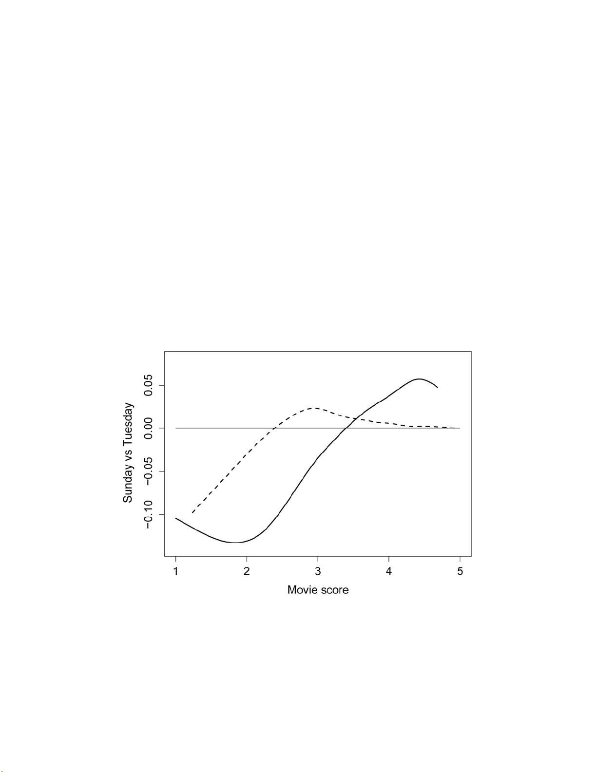
The Annals of Applie d Statistics 2007, V ol. 1, No. 2, 386–411 DOI: 10.1214 /07-A OAS122 c  Institute of Mathematical Statistics , 2 007 THE PIGEONHOLE BOOTSTRAP 1 By Ar t B. O wen Stanfor d University Recently there has b een muc h interest in data that, in statistical language, ma y be described as ha ving a large crossed and severely unbalanced random effects structure. S uch data sets arise for rec- ommender en gines and information retriev al problems. Many large bipartite w eighted graphs ha ve th is structu re too. W e w ould like to assess the stabilit y of algorithms fit to such data. Even for linear statistics, a naive form of b o otstrap sampling can b e seriously mis- leading and McCullagh [ Bernoul li 6 (2000) 285–301] has show n that no b o otstrap method is exact. W e sho w that an alternative bo otstrap separately resampling rows and columns of th e data matrix satisfies a mean consistency prop erty even in heteroscedastic crossed unbal- anced random effects mo dels. This alternative d oes not require the user to fit a crossed random effects mod el to t h e data. 1. In trod uction. Man y imp ortan t statistical problems feature t wo inter- lo c king sets of en tities, customarily arranged as r ows and columns. Unlik e the usual ca ses b y v aria bles la yo ut, these data fit b etter in to a cases by cases in terp r etation. Examples include b o oks and cu s tomers for a we b site, mo vies and raters for a recommender engine, and terms and do cuments in information retriev al. Historically data with this stru cture has b een studied with a crossed ran d om effects mo d el. Th e new data s ets are ve ry large and haphazardly structured, a far cry from the setting for whic h normal the- ory random effects mo dels w ere develo p ed. It can b e hard to estimate the v ariance of features fit to data of this kind. P arametric likelihoo d and Ba yesia n metho d s t ypically come with their o wn internally v alid metho d s of estimating v ariances. Ho wev er, th e crossed random effects setting can b e more complicated than what our mo dels an- ticipate. If in I ID sampling we sus p ect that ou r mod el is in adequate, then w e can mak e a simple and direct chec k on it via b o otstrap resampling of Received May 2007; revised Ma y 2007. 1 Supp orted by NSF Grant DMS- 06-04939. Key wor ds and phr ases. Collaborative fi ltering, recommenders, resampling. This is a n ele ctronic reprint o f the orig ina l ar ticle published by the Institute of Ma thematical Statistics in The Annals of Applie d Statist ics , 2007, V ol. 1, No. 2, 3 86–41 1 . This repr in t differs from the o riginal in pag ination and typogra phic detail. 1 2 A. B. OWEN cases. W e can ev en judge sampling uncertaint y for computations th at w ere not d eriv ed from any explicit mo del. W e would like to ha ve a v ersion of the b o otstrap su itable to large un- balanced crossed ran d om effect data sets. Unfortun ately for those hop es, McCullagh ( 2000 ) has p ro ved that no suc h b o otstrap can exist, ev en for the basic pr oblem of fin ding the v ariance of the grand mean of the data in a balanced setting with no m iss ing v alues and homoscedastic v ariables. McCullagh ( 2000 ) includ ed t wo reasonably well p erformin g appr o ximate metho ds for balanced data sets. Th ey yielded a v ariance that w as nearly correct u nder reasonable assump tions ab out the pr oblem. On e approac h wa s to fit the random effects mo del and then resample from it. Th at option is not attractiv e for the kind of data set considered here. Ev en an o ve r simplified mo del can b e hard to fit to u n b alanced data, and the results will lac k th e face v alue v alidit y that w e get from the b o otstrap for the I ID case. T h e second m etho d resampled r o ws and columns indep endent ly . T his appr oac h imitates th e Cornfield and T uke y ( 1956 ) pigeonhole sampling mo d el, and is preferable op erationally . W e call it th e pigeonhole b o otstrap, and sh o w that it contin ues to b e a reasonable estimator of v ariance ev en for s eriously unbala n ced data sets and inhomogenous (nonexchangea ble) random effects mo dels. In notation to b e explained further b elo w, w e fin d that the true v ariance of our statistic tak es the form ( ν A σ 2 A + ν B σ 2 B + σ 2 E ) / N , wh ere ν A and ν B can b e calculated f rom the data and s atisfy 1 ≪ ν ≪ N in our motiv ating applications. A naiv e b o otstrap (resampling cases) will p ro duce a v ariance estimate close to ( σ 2 A + σ 2 B + σ 2 E ) / N and th u s b e seriously misleading. Th e pigeonhole b o otstrap will p ro duce a v ariance estimate close to (( ν A + 2) σ 2 A + ( ν B + 2) σ 2 B + 3 σ 2 E ) / N . It is th u s mild ly conserv ative , but not u nduly so in cases where eac h ν ≫ 2 and σ 2 E do es not dominate. McCullagh ( 2000 ) lea ve s op en the p ossibilit y that a linear com bination of sev eral b o otstrap m etho ds w ill b e su itable. In the present setting the pigeonhole b o otstrap o ve r estimates the v ariance by t wice the amoun t of the n aiv e b o otstrap. On e could therefore b o otstrap b oth wa ys and su b tract t wice the n aive v ariance from the p igeonhole v ariance. That approac h, of course, b r ings the usual difficulties of p ossibly negativ e v ariance estimates. Also, sometimes w e do not wan t th e v ariance p er se, just a h istogram th at w e think has appro ximately the right width , and the v ariance is on ly a con- v enient w ay to decide if a h istogram has roughly the right width. Simply accepting a b o otstrap histogram that is sligh tly to o wide ma y b e prefer- able to trying to mak e it narro wer b y an amount based on the n aive v ari- ance. Man y of the motiv ating pr oblems come from e-commerce. There one m a y ha ve to d ecide where on a w eb page to place an ad or wh ich b o ok to recom- mend. Because the data sets are so large, coarse granularit y statistics can b e PIGEONHOLE BOOTSTRAP 3 estimated with essen tially negligible samp lin g u n certain t y . F or example, the Netflix data set has o ver 100 million movie ratings and the av erage mo vie rating is v ery w ell determined. Finer, subtle p oin ts, suc h as wh ether classical m u sic lo v ers are more likel y to pu r c hase a Harry Pott er b o ok on a T uesd a y are a different matter. S ome of these m a y b e we ll d etermin ed and some will not. An e-commerce application can ke ep trac k of millions of sub tle rules, and the small adv antag es so obtained can add up to something commercially v aluable. Thus, the dividing lin e b et w een noise artifacts and real s ignals is w orth fi nding, ev en in problems with large data sets. The outline of this pap er is as follo ws. Section 2 in tro duces the notation for ro w and column entiti es and sample sizes, includ in g the critical quan tities ν A and ν B , as w ell as the r andom effects mo del we consid er and the linear statistics we inv estigate. Section 3 int ro duces t w o b o otstrap mo dels: the naiv e b o otstrap and the p igeonhole b o otstrap. S ection 4 derives the v ariance expressions we need. Section 5 pr esen ts a small example, usin g the b o otstrap to determin e w h ether movie ratings at Netflix that we r e m ade on a T uesd ay really are lo wer than those fr om other da y s . There is a discu s sion in S ection 6 including application to mo dels u s ing outer p ro ducts as commonly fit b y the SVD. The App end ix con tains th e p ro of of Th eorem 3 . Shorter pro ofs app ear inline, b ut can b e easily skipp ed o ve r on fi rst reading. 2. Notatio n. Th e ro w en tities are i = 1 , . . . , R and the column entit ies are j = 1 , . . . , C . The v ariable Z ij ∈ { 0 , 1 } tak es the v alue 1 if w e ha ve data for th e ( i, j ) combinatio n and is 0 otherwise. Th e v alue X ij ∈ R d holds the observ ed data when Z ij = 1 and otherwise it is missin g. T o hide inessential details w e will work with d = 1, apart fr om a r emark in Section 4.4 . The data are X ij for i = 1 , . . . , R and j = 1 , . . . , C f or those ij pairs with Z ij = 1. T h e n um b er of times that ro w i was seen is n i • = P C j =1 Z ij . Similarly , column j wa s seen n • j = P R i =1 Z ij times. The total sample size is N = n •• = P i P j Z ij . In add ition to the R × C la y out with miss ing entries d escrib ed ab o ve, w e can also arr an ge the d ata as a sparse matrix via an N × 3 arr a y S with ℓ th ro w ( I ℓ , J ℓ , X ℓ ) for ℓ = 1 , . . . , N . The v alue X ℓ in th is lay out equals X I ℓ J ℓ from the R × C la y out. Th e v alue I ℓ = i app ears n i • times in column 1 of S , and similarly , J ℓ = j app ears n • j times in column 2. The ratios ν A ≡ 1 N R X i =1 n 2 i • and ν B ≡ 1 N C X j =1 n 2 • j , pro ve to b e imp ortant later. Th e v alue of ν A is the exp ectation of n i • when i is samp led with probabilit y prop ortional to n i • . If t wo not necessarily distinct ob s erv ations h a ving the same i are called “ro w n eigh b ors ,” then ν A 4 A. B. OWEN is the av erage num b er of row n eigh b ors for observ ations in the data set. Similarly , ν B is th e a verag e num b er of column neigh b ors. In the extreme where no column has b een seen t wice, eve ry n • j = 1 and then ν B = 1. I n the other extreme where there is only one column, ha ving n • 1 = N , then ν B = N . T ypically encounte red problems should h a ve 1 ≪ ν B ≪ N and 1 ≪ ν A ≪ N . F or example, an R × C table w ith no missin g v alues h as ν B = C and w e ma y exp ect b oth R and C to b e large. Often there will b e a Zipf-lik e distrib ution on n • j , and then for large p roblems w e will find that 1 ≪ ν B ≪ N . Similarly , cases with 1 ≪ ν A ≪ N are to b e exp ected. F or the Netflix d ata set, ν for customers is ab out 646 and ν for mo vies is ab out 56 , 200. As we will see b elo w , these large v alues mean that naiv e sampling mo dels seriously und erestimate the v ariance. W e also need the quantitie s µ • j ≡ 1 N X i Z ij n i • and µ i • ≡ 1 N X j Z ij n • j . Here µ • j is the pr obabilit y that a rand omly c hosen data p oin t has a “row neigh b or” in column j and an analogous interpretati on holds for µ i • . I f column j is full, then µ • j = 1. Ordinarily we exp ect that most, and p erhaps ev en all, of the µ • j will b e small, and similarly for µ i • . 2.1. R andom effe ct mo del. W e consider the d ata to hav e b een generated b y a mod el in whic h the pattern of observ ations has b een fixed, bu t those observ ed v alues m ight ha ve b een different. That is, Z ij are fixed v alues for i = 1 , . . . , R and j = 1 , . . . , C . T he mo del has X ij = µ + a i + b j + ε ij , (1) where µ is an un kno wn fixed v alue and a i , b j and ε ij are ran d om. In a classical random effects mo del (see Searle, Casella and McCullo ch ( 1992 ), Ch ap ter 5) we supp ose that a i ∼ N (0 , σ 2 A ), b j ∼ N (0 , σ 2 B ) and ε ij ∼ N (0 , σ 2 E ) all ind ep endently . W e relax the mo d el in several w ays. By tak- ing a i ∼ (0 , σ 2 A ) for i = 1 , . . . , R , we mean th at a i has mean 0 and v ariance σ 2 A but is not necessarily n ormally distr ibuted. Similarly , w e sup p ose that b j ∼ (0 , σ 2 B ) and that ε ij ∼ (0 , σ 2 E ). W e r efer to this mo del b elo w as the ho- mogenous ran d om effects mo d el. The homogenous rand om effects m o del is a type of “sup erp opulation” mo del as often used for samp ling fin ite p op- ulations. In a sup erp opu lation mo del we s upp ose that a large b u t finite PIGEONHOLE BOOTSTRAP 5 p opulation is itself a sample fr om an infinite p opulation that we wan t to study . Next, there ma y b e some measured or laten t attribu tes making a i more v ariable than a i ′ , for i 6 = i ′ . W e allo w for this p ossibilit y by taking a i ∼ (0 , σ 2 A ( i ) ), where σ 2 A (1) , . . . , σ 2 A ( R ) are v ariances sp ecific to the row en tities. Similarly , b j ∼ (0 , σ 2 B ( j ) ) and ε ij ∼ (0 , σ 2 E ( i,j ) ). The v ariables a i , b j and ε ij are m u tu ally in dep endent. That condition can b e r elaxed somewhat, as describ ed in Section 6 . The c hoice to mo del conditionally on th e observ ed Z ij v alues is a prag- matic one. The actual mec hanism generating the obs er v ations can b e v ery complicated. It in cludes th e p ossibilit y that an y particular ro w or column sum migh t sometimes b e p ositiv e and sometimes b e zero. By conditioning on Z ij , we a vo id having to mo del un ob s erv ed en tities. Also, in practice, one often fi nds that the smallest entiti es ha v e b een tr u ncated out of the data in a pr epro cessing step. F or example, r o ws might b e r emo v ed if n i • is b elo w a cutoff lik e 10. A column en tit y that is p opular with the small ro w ent ities migh t b e seriously affected, p erh ap s ev en to the p oin t of falling b elo w its o wn cutoff lev el. Similarly , the large en tities are sometimes remo ve d, bu t for d ifferen t reasons. In information retriev al, one often remo v es extremely common “stop words” lik e “and,” “of ” and “the” from the data. W orking conditionally lets us a void mo d eling this sort of truncation. 2.2. Line ar statistics. W e fo cus on a simple mean ˆ µ x = 1 N X i X j Z ij X ij = 1 N N X ℓ =1 X ℓ . A b o otstrap method that giv es th e correct v ariance for a mean can b e ex- p ected to b e reliable for more complicated statistics such as differences in means, other smo oth fu nctions of means and estimating equation parameters ˆ θ defined via 0 = 1 N X i X j Z ij f ( X ij , ˆ θ ) = 1 N N X ℓ =1 f ( X ℓ , ˆ θ ) . Con versely , a b o otstrap m etho d that do es not work reliably for linear statis- tics like a m ean cannot b e tru sted for m ore complicated usages. Lemma 1. Under the r andom effe cts mo del describ e d ab ove, V RE ( ˆ µ x ) = 1 N 2 R X i =1 n 2 i • σ 2 A ( i ) + C X j =1 n 2 • j σ 2 B ( i ) + R X i =1 C X j =1 Z ij σ 2 E ( i,j ) ! . (2) 6 A. B. OWEN Under the homo genous r andom effe cts mo del, V RE ( ˆ µ x ) = ν A σ 2 A N + ν B σ 2 B N + σ 2 E N . (3) Pr oof. Because th e a i , b i and ε ij are u n correlated, V RE ( ˆ µ x ) = V RE 1 N R X i =1 C X j =1 Z ij ( µ + a i + b j + ε ij ) ! = V RE 1 N R X i =1 n i • a i ! + V RE 1 N C X j =1 n • j b i ! + V RE 1 N R X i =1 C X j =1 Z ij ε ij ! , whic h reduces to ( 2 ). In the homogenous case ( 2 ) fur ther red u ces to ( 3 ).  In the nonhomogenous case, the un equal v ariance contributions for ro w en tities are weig hted prop ortionally to n 2 i • . T h u s, when the frequent en tities are more v ariable than the others, care m u st b e taken estimating v ariance comp onen ts for the h omogenous mo del. Using a p o oled estimate ˆ σ 2 A that w eights entities equally w ould lead to an underestimate of the v ariance of ˆ µ x . 3. Bo otstrap metho ds. W e would lik e to b o otstrap the data in such a w ay that th e v ariance of the b o otstrap resampled v alue ˆ µ ∗ appro ximates V RE ( ˆ µ x ). Even b etter, we would like to do this w ithout h a ving to mo d el the details of the r andom effects in v olv ed in X ij and without ha ving to exp licitly accoun t for the v arying n i • v alues. Here w e define a naiv e b o otstrap, wh ic h treats the data as I ID, and the pigeonhole b o otstrap. The latter resamples b oth r o ws and columns. Neither of th ese b o otstraps faithfu lly imitates the rand om effects mec hanism gener- ating th e data. Also, n either of them holds fixed th e sample sizes n i • and the latter d o es not even hold N fixed. T hus b oth b o otstraps m ust b e tested to see whether they yield a s erious systematic error. 3.1. Naive b o otstr ap. The u sual b o otstrap pr o cedure resamples the data I ID fr om th e empirical distrib ution. It can b e reliable even when the u nder- lying generativ e mo d el fails to hold. F or example, in I ID regression mo dels, resampling the cases give s reliable inferences for a regression parameter ev en when th e regression errors h a ve u nequal v ariance. It would b e naiv e to apply I I D resampling of the N observ ed d ata p oints to th e random effects setting, b ecause the X ij v alues are not indep end en t. Under s uc h a naiv e b o otstrap, ( I ∗ ℓ , J ∗ ℓ , X ∗ ℓ ) is d ra wn indep end en tly and u ni- formly fr om the N rows of S , for ℓ = 1 , . . . , N . Then ˆ µ ∗ x = 1 N N X ℓ =1 X ∗ ℓ . PIGEONHOLE BOOTSTRAP 7 Lemma 2. The exp e c te d value in the r andom effe cts mo del of the naive b o otstr ap varianc e of ˆ µ ∗ x is E RE ( V NB ( ˆ µ ∗ x )) , which is e qu al to 1 N 2 X i σ 2 A ( i ) n i •  1 − n i • N  (4) + 1 N 2 X j σ 2 B ( j ) n • j  1 − n • j N  + 1 N 2 X i X j Z ij σ 2 E ( i,j ) . Under the homo genous r andom effe cts mo del, E RE ( V NB ( ˆ µ ∗ x )) = σ 2 A N  1 − ν A N  + σ 2 B N  1 − ν B N  + σ 2 E N . (5) Pr oof. The naiv e b o otstrap v ariance of ˆ µ ∗ x is s 2 x / N , where s 2 x = (1 / N ) × P N ℓ =1 ( X ℓ − ˆ µ x ) 2 . Usin g the U -statistic formulati on, we ma y w rite it as V RE ( ˆ µ x ) = 1 2 N 3 N X ℓ =1 N X ℓ ′ =1 ( X ℓ − X ℓ ′ ) 2 = 1 2 N 3 X i X j X i ′ X j ′ Z ij Z i ′ j ′ ( a i − a i ′ + b j − b j ′ + e ij − e i ′ j ′ ) 2 . Then u nder the r andom effects mo del, E RE ( V NB ( ˆ µ x )) = 1 2 N 3 X i X j X i ′ X j ′ Z ij Z i ′ j ′ E ( a i − a i ′ + b j − b j ′ + e ij − e i ′ j ′ ) 2 = 1 2 N 3 X i X j X i ′ X j ′ Z ij Z i ′ j ′ (1 i 6 = i ′ ( σ 2 A ( i ) + σ 2 A ( i ′ ) ) + 1 j 6 = j ′ ( σ 2 B ( j ) + σ 2 B ( j ′ ) ) + (1 − 1 i = i ′ 1 j = j ′ )( σ 2 E ( i,j ) + σ 2 E ( i ′ ,j ′ ) )) = 1 N 2 X i σ 2 A ( i ) n i •  1 − n i • N  + 1 N 2 X j σ 2 B ( j ) n • j  1 − n • j N  + 1 N 2 X i X j Z ij σ 2 E ( i,j ) .  The homogenous case sho ws the differences clearly . The error term σ 2 E gets accoun ted for correctly , b ut not the other terms. Where the row v ariable really contributes ν A σ 2 A / N to the v ariance, the naive b o otstrap only captures σ 2 A (1 − ν A / N ) / N of it. It und erestimates this v ariance b y a factor of ν A / (1 − 8 A. B. OWEN ν A / N ) ≈ ν A , which ma y b e sub s tan tial. The v ariance due to the column v ariables is similarly under-estimated in the naiv e b o otstrap. 3.2. Pige onhole b o otstr ap. Th e naiv e b o otstrap fails b ecause it ignores similarities b et ween elemen ts of the same row and /or column. A more pr in- cipled b o otstrap would b e based on estimating the comp onen t parts of the random effects m o del, and resamp ling fr om it. Ho w ever, findin g a go o d wa y to estimate such a mo del can b e b urdensome. Normal th eory r andom effects mo dels for seve rely u n b alanced data sets are h ard to fit. More worryingly , the d ata ma y d epart seriously f rom normalit y , the v ariances σ 2 A ( i ) migh t b e nonconstan t, and could eve n b e correlated someho w with the samp le sizes n i • . The pigeonhole b o otstrap is n amed for a mo del used by Cornfield and T uke y ( 1956 ) to study balanced anov as with fi x ed , mixed and r andom effects. W e place the data in to an R × C m atrix, resample a set of rows, resample a s et of columns, and tak e the in tersections as the b o otstrapp ed data set. Th e original pigeonhole mo del inv olv ed sampling without rep lacement . The pi- geonhole b o otstrap samples with replacemen t. Th e app eal of the pigeonhole b o otstrap is that it generates a r esampled d ata set with v alues tak en from the original data. Th ere is n o need to form synthetic com binations of ro w and column en tities that were nev er observed together, n or resp onse v alues X ij that were not observ ed . F ormally , in the pigeonhole b o otstrap we sample rows r ∗ i I ID from U { 1 , . . . , R } for i = 1 , . . . , R and columns c ∗ j I ID fr om U { 1 , . . . , C } f or j = 1 , . . . , C . Ro ws and columns are sampled ind ep endently . The resampled data set h as Z ∗ ij = Z r ∗ i c ∗ j and when Z ∗ ij = 1, we tak e X ∗ ij = X r ∗ i c ∗ j . The b o otstrap sample sizes are n ∗ i • = P C j =1 Z ∗ ij , n ∗ • j = P R i =1 Z ∗ ij and N ∗ = n ∗ •• = P R i =1 P C j =1 Z ∗ ij . The b o otstrap pro cess ab o ve is rep eated in d ep endently , some num b er B of times. Ro w i = 1 in Z ∗ ij do es not ordinarily corresp ond to the same en tit y as ro w i = 1 in Z ij . Should w e wan t to ke ep trac k of the n u m b er of times that original r o w en tity r app eared in the resamp led data, we wo uld use e n ∗ r • = R X i =1 C X j =1 Z r ∗ i c ∗ j × 1 r ∗ i = r = R X i =1 n ∗ i • 1 r ∗ i = r . Similarly , column c app ears e n ∗ • c = P C j =1 n ∗ • j 1 c ∗ j = c times among the r esampled v alues. 4. V ariances. Here we d evelo p the v ariance f orm u las for pigeonhole b o ot- strap sampling. I t is conv enien t to consider the en tities as b elonging to a PIGEONHOLE BOOTSTRAP 9 large but fin ite set. Then we may w ork with p opulation totals, a concept that makes no sense for an in finite p o ol of entit ies. There are t wo uncertainti es in a b o otstrap v ariance estimate. On e is sam- pling uncertain t y , the v ariance un der b o otstrapping B times of our v ariance estimate. The other is s y s tematic uncertain ty , th e difference b et ween the exp ectation of our b o otstrap v ariance estimate and the v ariance we wish to estimate. W e fo cus on the latter b ecause th e resamplin g mo del differs f rom the one we assume has generated the data. The former issue can b e help ed b y increasing B , and will b e less sev ere for large N . It w ill b e p ossible to construct examples where sampling fl uctuations d ominate, but we do not consider that case here. McCullagh ( 2000 ) also c hose to compare exp ected b o otstrap v ariance to sampling v ariance. 4.1. V arianc e of totals in pige onhole b o otstr ap. The total v alue of X o ver the samp le is T x = P i P j Z ij X ij . In b o otstrap sampling, the tota l of X ∗ is T ∗ x = P i P j Z ∗ ij X ∗ ij . Lemma 3. Under pige onhole b o otstr ap sampling, E PB ( T ∗ x ) = T x and E PB ( N ∗ ) = N . Pr oof. First, E ( T ∗ x ) = P R i =1 P C j =1 E B ( Z ∗ ij X ∗ ij ) = RC E PB ( Z ∗ 11 X ∗ 11 ) by sym - metry . The fi rst result then follo ws b ecause E PB ( Z ∗ 11 X ∗ 11 ) = 1 / ( RC ) P i P j Z ij × X ij . The second result follo ws on putting N = T z and N ∗ = T ∗ z and consid- ering th e case X ij = Z ij .  Theorem 1. Under pige onhole b o otstr ap sampling, V PB ( T ∗ x ) =  1 RC − 1 R − 1 C  T 2 x +  1 − 1 C  X i T 2 xi • +  1 − 1 R  X j T 2 x • j + X i X j Z ij X 2 ij , wher e T xi • = P C j =1 Z ij X ij and T x • j = P R i =1 Z ij X ij . Pr oof. W e w rite E PB (( T ∗ x ) 2 ) = X i X j X i ′ X j ′ E PB ( Z ∗ ij X ∗ ij Z ∗ i ′ j ′ X ∗ i ′ j ′ ) and then split the s u m into four cases d ep ending on whether i = i ′ or n ot and wh ether j = j ′ or n ot. By symmetry , w e only need to consider i , j , i ′ 10 A. B. OWEN and j ′ equal to 1 or 2 . Thus, E PB (( T ∗ x ) 2 ) = R ( R − 1) C ( C − 1) E PB ( Z ∗ 11 X ∗ 11 Z ∗ 22 X ∗ 22 ) + RC ( C − 1) E PB ( Z ∗ 11 X ∗ 11 Z ∗ 12 X ∗ 12 ) + R ( R − 1) C E PB ( Z ∗ 11 X ∗ 11 Z ∗ 21 X ∗ 21 ) + RC E PB ( Z ∗ 11 X ∗ 11 Z ∗ 11 X ∗ 11 ) = R ( R − 1) C ( C − 1) T 2 x R 2 C 2 + R C ( C − 1) 1 RC 2 X i T 2 xi • + R ( R − 1) C 1 R 2 C X j T 2 x • j + R C 1 RC X i X j Z ij X 2 ij , whic h , combined with Lemma 3 , yields the result.  4.2. R atio e stimation. The simple mean of X is ˆ µ x = T x / N . Under b o ot- strap resampling, we generate ˆ µ ∗ x = T ∗ x / N ∗ . The mean and v ariance of ˆ µ ∗ x are complicated b ecause they are ratios. The b o otstrap samp le size N ∗ , app earing in the denominator, is not constan t. There is a standard wa y to handle ratio estimators in sampling theory [ Co c h r an ( 1977 )]. It amounts to use of the delta metho d . The approximate v ariance of ˆ µ ∗ x using ratio estimation tak es the form ˆ V PB ( ˆ µ ∗ x ) = 1 N 2 E PB  T ∗ x − T x N N ∗  2  . (6) Theorem 2. Under pige onhole b o otstr ap sampling, ˆ V PB ( ˆ µ ∗ x ) = 1 N 2 "  1 − 1 C  X i n 2 i • ( ¯ X i • − ˆ µ x ) 2 +  1 − 1 R  X j n 2 • j ( ¯ X • j − ˆ µ x ) 2 + X i X j Z ij ( X ij − ˆ µ x ) 2 # , wher e ¯ X i • = P C j =1 Z ij X ij /n i • and ¯ X • j = P R i =1 Z ij X ij /n • j . Pr oof. Let Y ij = X ij − T x Z ij / N when Z ij = 1. T h en T y = T x − T x T z / N = 0 . Also, T ∗ y = T ∗ x − T x N ∗ / N an d so E PB (( T ∗ x − T x N ∗ / N ) 2 ) = V PB ( T ∗ y ). F rom Th eorem 1 app lied to Y in stead of X w e hav e ˆ V PB ( ˆ µ ∗ x ) = 1 N 2 "  1 − 1 C  X i T 2 y i • +  1 − 1 R  X j T 2 y • j + X i X j Z ij Y 2 ij # . PIGEONHOLE BOOTSTRAP 11 W e fi nd th at X ij − Z ij T x / N = X ij − ˆ µ x whenev er Z ij = 1, and so X i T 2 y i • = X i X j Z ij ( X ij − Z ij T x / N ) ! 2 = X i X j Z ij ( X ij − ˆ µ x ) ! 2 = X i n 2 i • ( ¯ X i • − ˆ µ x ) 2 and a similar expression h olds for P i T 2 y i • . Also, X i X j Z ij Y 2 ij = X i X j Z ij ( X ij − ˆ µ x ) 2 .  Next w e study the exp ected v alue under the rand om effects m o del of the b o otstrap v ariance ˆ V PB ( ˆ µ ∗ x ). W e get an exact but length y formula and then apply simp lifications. Theorem 3. The exp e cte d value under the r andom effe cts mo del of the pige onhole varianc e is E RE ( ˆ V PB ( ˆ µ ∗ x )) = 1 N 2 " X i σ 2 A ( i ) λ A i + X j σ 2 B ( j ) λ B j + X i X j Z ij σ 2 E ( i,j ) λ E i,j # , wher e λ A i =  1 − 1 C  n 2 i •  1 − 2 n i • N + ν A N  +  1 − 1 R  n i • − 2 µ i • n i • + ν B n 2 i • N  + n i •  1 − n i • N  2 + n 2 i • N 2 ( N − n i • ) , λ B j =  1 − 1 R  n 2 • j  1 − 2 n • j N + ν B N  +  1 − 1 C  n • j − 2 µ • j n • j + ν A n 2 • j N  + n • j  1 − n • j N  2 + n 2 • j N 2 ( N − n • j ) , and for Z ij = 1 , λ E i,j =  1 − 1 C  1 − 2 n i • N + ν A N  +  1 − 1 R  1 − 2 n • j N + ν B N  + 1 − 1 N . Pr oof. See th e App end ix . The v ariance expression ab o ve is unwieldy . W e use the n otatio n ≈ to indicate that terms lik e 1 /R , 1 /C , n i • / N , n • j / N , ν A / N , ν B / N , µ i • and µ • j are considered n egligible compared to 1, as they u sually are in the motiv ating 12 A. B. OWEN applications. W e do not su pp ose that n i • /n 2 i • is negligible b ecause some or ev en most of the n i • could b e small. Under these conditions, λ A i ≈ n 2 i • + 2 n i • , λ B j ≈ n 2 • j + 2 n • j and for Z ij = 1 , λ E i,j ≈ 3 . Corollar y 1. E RE ( ˆ V PB ( ˆ µ ∗ x )) ≈ 1 N 2 " X i σ 2 A ( i ) ( n 2 i • + 2 n i • ) (7) + X j σ 2 B ( j ) ( n 2 • j + 2 n • j ) + 3 X i X j Z ij σ 2 E ( i,j ) # , and under the homo g enous r andom effe cts mo del, E RE ( ˆ V PB ( ˆ µ ∗ x )) ≈ 1 N ( σ 2 A ( ν A + 2) + σ 2 B ( ν B + 2) + 3 σ 2 E ( i,j ) ) . Pr oof. E RE ( ˆ V PB ( ˆ µ ∗ x )) = 1 N 2 " X i σ 2 A ( i ) λ A i + X j σ 2 B ( j ) λ B j + X i X j Z ij σ 2 E ( i,j ) λ E i,j # ≈ 1 N 2 " X i σ 2 A ( i ) ( n 2 i • + 2 n i • ) + X j σ 2 B ( j ) ( n 2 • j + 2 n • j ) + 3 X i X j Z ij σ 2 E ( i,j ) # . The sp ecializat ion to the homogenous case follo ws easily .  The v ariance con tr ib ution from ε ij is o verestimat ed b y a f actor of 3 in the pigeonhole b o otstrap. In the homogenous case this o v erestimate is not imp ortant when σ 2 E ≪ m ax( ν A σ 2 A , ν B σ 2 B ). When ν A and ν B are large, it only tak es a small amoun t of v ariation in σ 2 A and σ 2 B to m ak e σ 2 E unimp ortan t. A similar conclusion follo ws for the inhomogenous case in terms of appr o- priately weig h ted a v erages of the v ariances. The a verag e v alue of the v ariance in equation ( 7 ) trac ks ve ry closely with the desired rand om effects v ariance of ˆ µ x giv en by ( 2 ), eve n when the effects PIGEONHOLE BOOTSTRAP 13 are h eteroscedastic . Wher e the latter h as n 2 i • , th e form er has n 2 i • + 2 n i • , an d similarly for n 2 • j . O u tside of extreme cases P i n i • σ 2 A ( i ) ≪ P i n 2 i • σ 2 A ( i ) . In some applications some or man y of the µ i • and µ • j ma y b e nont rivially large. In recommender settings, a small num b er of b o oks or mo v ies ma y h a ve b een r ated b y a large fraction of p eople, or s ome p eople ma y ha ve r ated an astonishingly large num b er of items. I n information r etriev al, some terms migh t app ear in most do cuments, as, for example, when we c h o ose to retain the stop wo r ds. Und er such cond itions, we get a sligh t v ariance reduction: λ A i ≈ n 2 i • + 2(1 − µ i • ) n i • and λ B j ≈ n 2 • j + 2(1 − µ • j ) n • j , while λ E i,j remains app ro ximately 3. But wh en µ i • is not small, then w e may reasonably exp ect n i • to b e large and n 2 i • ≫ n i • . Thus, the approxi mation in Corollary 1 is still appropriate. 4.3. Me an c onsistency. The expr ession ≈ conv eys what we ordinarily exp ect to b e the imp ortan t terms . W e fi nd E RE ˆ V PB ( ˆ µ ∗ x ) ≈ V RE ( ˆ µ x ) or E RE ˆ V PB ( ˆ µ ∗ x ) /V RE ( ˆ µ x ) ≈ 1 . Ho w ever, the earlier section left op en th e p os- sibilit y of extreme cases where P i n i • σ 2 A ( i ) w as not negligible compared to P i n 2 i • σ 2 A ( i ) . F or example, supp ose that σ 2 A ( i ) = 0 for all i w ith n i • > 1. Th en ( n 2 i • + 2 n i • ) σ 2 A ( i ) = 3 n 2 i • σ 2 A ( i ) and the pigeonhole b o otstrap could essentiall y triple th e v ariance contribution from the row ent ities. T o formulate “mean consistency” of ˆ V PB ( ˆ µ ∗ x ) more carefully , we d efine ǫ N = max  1 R , 1 C , ν A N , ν B N , 1 ν A , 1 ν B , max i n i • N , max j n • j N  , (8) and work in the limit as N → ∞ w ith ǫ N → 0. Arranging the terms in eac h λ , w e get λ A i = n 2 i • (1 + O ( ǫ N )) + 2 n i • (1 − µ i • )(1 + O ( ǫ N )) , λ B j = n 2 • j (1 + O ( ǫ N )) + 2 n • j (1 − µ • j )(1 + O ( ǫ N )) and λ E i,j = 3 + O ( ǫ N ) , where th e implied constan t in all th e O ( ǫ N ) terms is indep en den t of i and j . T o ru le out pathological heteroscedasticit y , w e sup p ose that 0 < m A ≤ σ 2 A ( i ) ≤ M A < ∞ , 0 < m B ≤ σ 2 B ( j ) ≤ M B < ∞ 14 A. B. OWEN and 0 < m E ≤ σ 2 E ( i,j ) ≤ M E < ∞ holds for all 1 ≤ i ≤ R = R ( N ) and 1 ≤ j ≤ C = C ( N ). Theorem 4. Supp ose that σ 2 A ( i ) , σ 2 B ( j ) and σ 2 E ( i,j ) ob e y the b ounds ab ove, and that ǫ N → 0 as N → ∞ . Then E ( V PB ( ˆ µ x )) − V RE ( ˆ µ x ) V RE ( ˆ µ x ) = O ( ǫ N ) . Pr oof. Gathering u p the pieces, E ( V PB ( ˆ µ x )) − V RE ( ˆ µ x ) V RE ( ˆ µ x ) = O ( ǫ N ) + 2(1 + O ( ǫ N )) × ρ N , where ρ N = P i n i • (1 − µ i • ) σ 2 A ( i ) + P j n • j (1 − µ • j ) σ 2 B ( j ) + P i P j Z ij σ 2 E ( i,j ) P i n 2 i • σ 2 A ( i ) + P j n 2 • j σ 2 B ( j ) + P i P j Z ij σ 2 E ( i,j ) . The numerator of ρ N lies b et ween N m E and N ( M A + M B + M E ), while th e denominator is at least N ( ν A m A + ν B m B + m E ). Therefore, 0 ≤ ρ N ≤ M A + M B + M E ν A m A + ν B m B + m E = O ( ǫ N ) .  4.4. Covarianc es. The v ariance expressions in this p ap er generalize in an uns u rprising wa y to co v ariances of p airs of resp onses. Th e simp lest w ay to express this is to supp ose that X ij ∈ R d . Then we may generalize σ 2 A ( i ) , σ 2 B ( j ) and σ 2 E ( i,j ) to b e d × d co v ariance matrices. Th e v ariance form u las go through as ab o ve. Expr essions like P i n i • σ 2 A ( i ) ≪ P i n 2 i • σ 2 A ( i ) then mean that P i n i • u ′ σ 2 A ( i ) u ≪ P i n 2 i • u ′ σ 2 A ( i ) u for all u ∈ R d with k u k = 1. 5. Netflix movie ratings example. As an example of a small effect n ear the u ncertain t y level , w e consider the da y of the we ek effect in mo vie rat- ings for the Netflix data. Th is d ata set is describ ed and is av ailable from http://w ww.netfli xprize.com/index . It has 100,4 80,507 ratings on 17,770 mo vies from 480,189 customers. As ment ioned ab o ve, ν for cu s tomers is ab out 646 and ν for mo vies is ab out 56,200. The num b er of r atings p er customer ranges fr om 1 to 17,653. Th e num b er of ratings for mo vies ranges from 3 to 232,944. PIGEONHOLE BOOTSTRAP 15 5.1. Day of the we ek effe ct. It w ould b e inte resting to examine the effects of demographic v ariables on mo vie ratings, but for priv acy p u rp oses those are n ot included in the data. T he data set do es, ho w ever, sup ply a date for eac h r ating. F or eac h day of the w eek, w e may find the a verag e mo vie rating giv en out. The smallest v alue is 3 . 595808 for T u esda ys and the largest is 3 . 6164 49 f or Sun da ys. Th e da y of the w eek effect is v ery small. P erh aps the mo vie ratings giv en out on Sund a y do tend to b e larger than th ose giv en out on Su nda y . If so, w e migh t in vestig ate whether this arises from a different mix of mo vies b eing rated that day , a different set of customers r ating on th at da y , or some subtle int eraction. But b efore doing suc h follo wu p, w e should c hec k w hether the difference migh t just b e a samplin g flu ctuation. F or su c h a large d ata set, samp ling fl u ctuations are exp ected to b e small. But th e observ ed effect is also qu ite s m all, and the sampling fluctuations include rand om effects from movies and customers that can mak e them muc h larger than w e were used to in the I I D setting. Figure 1 shows results for 10 pigeonhole b o otstrap samples. In eac h sample the means for all 7 da ys of the w eek were recorded. There is clearly a b ias in the b o otstrap resampling. Th e a ve rage score on any giv en d ay in resampling is a ratio estimate of the total of all scores giv en for that day d ivid ed b y the n u m b er of ratings for that day . T he bias is very small in absolute terms, bu t not compared to th e pigeonhole b o otstrap standard deviation. A da y versus da y comparison is more inte resting than the absolute lev el for a give n da y . T o compare T uesda y and S unday , we lo ok at the 10 paired a ve rage s cores. Th ese are shown in Figure 2 . Th e solid p oint is 0 . 0206 u nits ab o ve the f ort y-five degree line, ind icating that Su n da y scores a verage that m u c h higher than T uesday s cores. The r esampled p oin ts a v erage 0 . 0214 u nits ab o ve the line. This is v ery close to the sample difference. The biases for the tw o d ays’ scores hav e almost completely cancelled out, so that some resampled p oin ts are farther from the line than the original p oin t while others are closer. T he av erage resamp led d ifferen ce in means is ab out 8 . 16 times as large as the standard deviation of the resampled differences. The 10 b o otstrap differences are indep end en t, and should b e nearly normal b ecause of th e large samp le sizes inv olv ed. Then P r( | t (9) | ≥ 8 . 16) . = 1 . 88 × 10 − 5 . T his is small enough for us to conclude that the difference is real, ev en if we tak e account of ha ving selected the most significant of all 21 da y to da y comparisons. 5.2. Par ameters and hyp othesis. This section mak es clear wh at hyp oth- esis is b eing tested b y the b o otstrap analysis and w h at are the un derlying parameters. Then it looks at ho w w ell the ran d om effects mod el might fit the p resen t setting. Let Y ij b e the score for a movie and let Z ij b e an indicator that it w as observ ed . Intro duce binary co v ariates D T ue ij taking the v alue 1 if and only if 16 A. B. OWEN Fig. 1. The horizontal axis depicts the day of the we ek fr om Monday at 0 to Sunday at 6 . The vertic al axis has aver age movie r ating sc or es. F or e ach day the solid dot shows that day’s aver age movie r ating in the original data set. The op en dots show the aver age in e ach of 10 pige onhole b o otstr ap samples. the ij measurement happ ened on T u esd a y . Similarly , let D Sun ij b e the d a y of w eek in dicator for Sund a y . The sample a verag e for T uesda y is ˆ µ T ue = P ij Z ij D T ue ij Y ij P ij Z ij D T ue ij (9) and ˆ µ Sun is defin ed s imilarly . W e in terp ret ˆ µ T ue ab o ve as an estimate of µ T ue = E RE ( P ij Z ij D T ue ij Y ij ) E RE ( P ij Z ij D T ue ij ) , (10) so that µ T ue is th e solution to E RE ( P ij Z ij D T ue ij ( Y ij − µ T ue )) = 0 . The null h yp othesis H 0 b eing tested by the pigeonhole b o otstrap analysis is th at µ Sun − µ T ue = 0. In b o otstrapping ˆ µ T ue pla ys the role of the parameter and ˆ µ ∗ T ue pla ys th at of the estimate. The parameter µ T ue is well d efined so long as Pr( P ij Z ij D T ue ij = 0) > 0. W e ha v e neglecte d the p ossibilit y that the denominator in ˆ µ ∗ T ue is zero. In practice, one might add a small constan t to the denominator of eac h ˆ µ ∗ T ue , or condition on th e denominator b eing p ositiv e. Such small resampled PIGEONHOLE BOOTSTRAP 17 Fig. 2. The horizontal axis shows the aver age movie r ating given on T uesday. The ver- tic al axis shows Sunday. The op en cir cles ar e fr om 10 pige onhole b o otstr ap samples. The solid p oint is fr om the original data. F or e ach day the soli d dot shows that day ’ s aver- age movie r ating in the original data set. The op en dots show the aver age i n e ach of 10 b o otstr ap samples. denominators are, h o wev er, a s ign th at the delta metho d appro ximation for the v ariance of th e ratio ma y b e inaccurate. The simp lest path b et wee n the r andom effects mo del and the data set is to sup p ose that th e triple ( Y ij , D T ue ij , D Sun ij ) app ro ximately follo ws a crossed random effects mo d el of the form studied in this pap er. Suc h a mo del is somewhat u nnatural though, b ecause tw o of the v ariables are bin ary . All w e need, h o wev er, is that the first term in the linearization of the test statistic f ollo ws appro ximately a crossed r andom effects mo d el. The linearized statistic is not b inary . 18 A. B. OWEN Dropping the sub script an d su p erscript for T uesda y , and writing the ratio in ( 9 ) as T z dy /T z d , the delta metho d linearization of this ratio is µ + T z dy − E ( T z dy ) E ( T z d ) − T z d − E ( T z d ) E ( T z d ) 2 = const + X ij Z ij D ij ( Y ij E ( T z d ) − 1 − E ( T z d ) − 2 ) . The linearization for T uesd a ys tak es six d ifferen t v alues, corresp ond ing to fiv e different v alues when D T ue ij = 1 and one v alue for all cases with D T ue ij = 0. After linearizing the Sunday versus T uesda y difference, there are elev en differen t v alues arising as fiv e for Su nda y ratings, fiv e for T uesday ratings, and one for ratings mad e on the other five days. 5.3. A de ep er lo ok into the data . Sund a y ratings are ab out 0 . 02 p oin ts higher than T uesda y ratings. T his difference is small, but statistically sig- nifican t, eve n allo wing for random customer and mo vie effects. What follo ws is an informal data analytic exp loration of th e n ature of this discrepancy . Making the analysis formal w ould tak e us s omewhat b eyo nd the results pr o ve d here. Sev eral exp lanations f or the day of wee k effect are plausible. One is that the harder to please customers r ate more often on T uesday . A second is that a giv en customer making a rating su p plies a lo w er r ating if the da y is T u esda y . There are also v ersions of these explanations centered on mo vies. The m ovies rated on T uesda y migh t tend to b e less p opular, or a give n mo vie getting rated on a T uesd a y m igh t tend to get a lo wer rating than on a Su nda y . A simple proxy for how we ll a movie is like d is th e a v erage score it gets. Similarly , the generosit y lev el of a customer ma y b e jud ged b y the a v er age score that he or she giv es. Th ere were 17 , 784 , 852 T uesday ratings and the a ve rage o v er these r atings of our simple movie score is 3 . 6 00 (rounded to the nearest 1 / 1 000th), sligh tly higher than the simp le a v erage of all T ues- da y scores. Th e comparable num b ers for S unday are 10,730,35 0 and 3 . 616. Therefore, it app ears that slightl y more p opular mo v ies are b eing rated on Sund a ys than on T u esda ys. This simple analysis yields an estimated gap of 0 . 016 compared to the observ ed gap of 0 . 020. A customer-based version of this analysis yields a gap of on ly 0 . 010 (from 3 . 610 versus 3 . 600). By th is an alysis, the effect seems to b e due sligh tly more to whic h mo vies are b eing rank ed than to w ho is doing the ranking. If we add b oth effects, w e get a predicted gap of 0 . 026. This v alue is higher th an what w as observ ed, indicating that some amount of double coun ting is taking place. T h is d ouble coun ting is consistent with a str on g feature in the data. Popular mo vies get more ratings and also h igher ratings. V ery activ e customers giv e more PIGEONHOLE BOOTSTRAP 19 ratings, ha ve a harder time restricting th emselv es to ju st the p opu lar movie s, and, not sur prisingly , tend to giv e out lo w er r atings. T h u s, kn o wing that T u esda y has the less p opu lar mo vies already leads one to su sp ect it will ha ve the b usier and , hence, less generous customers. Another an alysis lo oks at customers who ga ve r atings on b oth T uesday and Su nda y . F or eac h suc h customer w e can measure their a v erage Su nda y rating and subtract their a v erage T uesday rating. Th is gives eac h customer a Sund a y ve rsus T uesday differentia l. The mean o v er customers of this dif- feren tial is 0 . 016. P erh aps coinciden tally , this matc hes the a verage mo vie effect. The mean o v er movie s of a comparable mo vie different ial is − 0 . 008. It h as an u nexp ected sign, meaning that by this measur e Sun da y scores are lo we r than T uesda y scores. A m ore prop er analysis u ses a w eigh ted a verag e of customers or movi es, with we ights dep end ing on h o w m an y data p oin ts they con tr ib ute. Th e prop er we igh ting ma y b e a matter of debate, but, for simplicit y , we u se the harmonic m ean of n T ue and n Sun where these are the n u m b er of T uesday and Sunday ratings made by the customer. Now the w eighte d mean different ial is 0 . 009. T aking this at f ace v alue, cu s tomers seem to b e sligh tly h arder to please on T u esd a y . A similar w eighte d analysis b y mo vies give s a d ifferential of 0 . 011, so mo vies tend to get lo wer scores on T u esda y . The pattern in the differentials is somewhat more subtle than the analysis ab o ve describ es. F or a giv en customer, let Y denote the a v erage of their Sund a y scores min us the a ve r age of their T u esda y scores and let X denote the simple av erage of those t wo av erage scores. A plot of Y v ersu s X has a great m any d ata p oin ts, bu t a spline smo oth, using the h armonic mean w eights describ ed ab o ve shows a pattern. Generous cu s tomers are eve n more generous on Sun da ys than T uesda ys . But hard to please customers giv e even lo we r ratings on S undays than T uesd ays. In other words, the customers are sligh tly m ore extreme on Su nda ys than they are on T u esda ys. Because high scores are more common, this raises the a ve rage score on Sun da y versus T uesda y . A comparable analysis by movi e sho w s that u np opu lar mo vies get eve n low er scores on T uesd a ys, p opular mo vies get ab out the same s core on b oth da ys, and in termediate mo vies get somewhat h igher scores on T uesdays. These cur ves are sh own in Figure 3 . The inf ormal data analysis ab o ve give s some supp ort to all four explana- tions offered. T uesd a y app ears to get m ore of the tougher cu stomers and the w eake r mo vies. F u rthermore, a giv en customer or mo vie seems to result in a lo wer score if the rating is made on T u esda y . F rom the figur e w e see that the within customer or w ith in movi e day of the week effect can b e p ositiv e or n egativ e and m ay b e m u c h larger than 0 . 002 in absolute v alue. 6. Discussion. Ultimately we wo u ld lik e to hav e a trust worth y b o otstrap analysis for elab orate method s such as the sp ectral biclusterin g pro cedur e 20 A. B. OWEN of Dhillon ( 2001 ), among others. Runn in g five or ten rep eats w ould giv e insigh t as to wh ic h features of the analysis remain s table and whic h ones migh t b e idiosyncratic to the data set at hand. T here is a large complexity gap b et ween the output of suc h metho ds and th e simple mean consid er ed here. It do es, ho we v er, seem reasonable to rule out metho ds that ca nnot handle the global m ean and fo cus further r esearc h on one that d o es. W e w ould also w ish to ha ve a b o otstrap th at w orks under more flexi- ble settings th an the additiv e random effects mo d el in ( 1 ). The rest of this discussion presen ts t wo simple generalizations of ( 1 ) w here th e pigeonhole b o otstrap can b e app lied and th en discusses the issue of b ias, and the dif- ference b et ween fixed and r andom Z ij mo dels. 6.1. R elaxing indep endenc e. It is not hard to see that the same v ariance results arise if the a i , b j and ε ij are simply un correlated and not n ecessarily indep end en t. This helps us in settings w here X ij m u st b e in a restricted set. Fig. 3. These curves show how the Sunday versus T uesday r ating differ enc e varies with the p opularity of movies. The solid curve shows an analysis by custo mers, the dashe d curve shows an analysis by movies. Supp ose that a customer makes n T u e ≥ 1 r atings on T uesday with aver age value ¯ Y T u e and simi larly for Sunday. Then the soli d curve i s a spline smo oth on 8 de gr e es of fr e e dom of ¯ Y Sun − ¯ Y T u e versus ( ¯ Y Sun + ¯ Y T u e ) / 2 over customers, with weights 2 / (1 /n Sun + 1 /n Sun ) . The dashe d curve is c ompute d the same way, using c ounts and aver ages p er movie. PIGEONHOLE BOOTSTRAP 21 F or example, if the X ij v alues can only b elong to a fi nite set, suc h as m ovie ratings { 1 , 2 , 3 , 4 , 5 } , then giv en a i and b j there are only 5 allo wable v alues for ε ij . Because these allo w able v alues dep en d on a i + b j the error ε ij cannot b e indep end en t of a i and b j . It can, h ow ev er, weigh t its allo w able v alues in suc h a wa y that E ( ε ij | a i , b j ) = 0 and V ( ε ij | a i , b j ) = σ 2 E ( i,j ) . Therefore, a mo del with ε ij m u tually ind ep endent from (0 , σ 2 E ( i,j ) ) cond itionally on a 1 , . . . , a R and b 1 , . . . , b C is plausible. In such a mo del the ε ij are uncorrelated with a i and b j . The relaxati on do es not go quite as far as we migh t w ant. F or example, if there is an upp er b ound on X ij , then the largest p ossible a i and largest p ossible b j m u st sum to at m ost that b ound , or else ε ij cannot h a ve mean 0 . 6.2. Outer pr o duct mo dels. W e migh t supp ose that in s tead of the additiv e rand om effects mo del, th at an outer pro d uct rep r esen tation is more appropriate. Su c h SVD t yp e m o dels hav e b ecome imp ortan t in in- formation r etriev al [ Deerw ester et al. ( 1990 )] and DNA microarra y analysis [ Alter, Bro wn and Botstein ( 2000 )]. Under such a mo d el w e wr ite X ij = µ + a i + b j + L X ℓ =1 λ ℓ u iℓ v j ℓ + ε ij , (11) where the n ew pieces are scalar singular v alues λ ℓ and the s ingular ve ctors with comp onent s u iℓ and v j ℓ . Ordinarily the singular vect ors are fit to th e data sub j ect to a n orm constraint . As a mo d el for ho w the data might hav e arisen, we don’t ha ve to imp ose that constrain t. W e can make the pieces random with u iℓ ∼ (0 , τ 2 U ( i,ℓ ) ), and v j ℓ ∼ (0 , τ 2 V ( j,ℓ ) ) indep endentl y of eac h other and the a i and b j . The mo d el ( 11 ) is p opular in crop science [ Cr ossa and C orn elius ( 2002 )] where the ro ws and column s corresp ond to genot yp es and en vir on m en ts. Surp r isingly , to mo d er n readers that mo del (with L = 1) is ab out as old as the earliest ANOV A p ap ers, going bac k to Fisher and Mac kenzie ( 1923 ). W riting η ij = L X ℓ =1 λ ℓ u iℓ v j ℓ + ε ij , w e find that η ij are uncorrelated with eac h other and with a i and b j . Un- correlated errors η ij lead to the same v ariances as ind ep endent ones d o. Therefore, w e can s u bsume rand omly generated outer pr o ducts int o the ε ij term of mo d el ( 1 ). As a consequence, we can app ly the pigeonhole b o otstrap without knowing what the v alue of L is, including the p ossibilit y th at L = 0 migh t b e the b est d escription of the data. 22 A. B. OWEN A v ery early outer pro d uct mo del is the one degree of freedom for non- additivit y of T u k ey ( 1949 ). In this mo del X ij = µ + a i + b j + λa i b j + ε ij . (12) It differs from the additive plus outer pr o duct mo d el in ha ving the same v ariables app ear in b oth places. Once again, we can sub s ume the outer pro du ct part into the error b ecause λa i b j + ε ij is u ncorrelated with a i , b j and λa i ′ b j + ε i ′ j when i 6 = i ′ , if all the a i , b j and ε ij are ind ep endent. 6.3. Bias. It is a commonplace that biases affect o verall lev els m uc h more than they affect comparisons. The EP A used to say ab out automobile effi- ciency that w hile “y our mileage may v ary” from what th ey rep ort, rep orted differences b et ween vehicle s should b e accurate. (No w they sa y “y our mpg wil l v ary .”) In practice w ith the b o otstrap, we would lik e to kno w wh ether a giv en statistic is p er f orming with bias lik e the T uesd a y score, or w ith muc h less b ias lik e the Su nda y versus T uesda y d ifference. F or a scalar p arameter w e can compare the resampled v alues to the original one. F or our hyp othetical b o okseller wo n dering wh ether classical music lo vers are more lik ely to pu rc hase a Harry P otter b o ok on a T uesda y , it no w b e- comes clear that “more lik ely than what?” is an imp ortant consideration. A con trast w ith other days, other b o oks or other customer t yp es will b e b etter determined than the absolute level. It would b e in teresting to know w hether the bias in the pigeonhole b o ot- strap tracks with the sampling bias in any reasonable generativ e mo d el ha v- ing r andom sample sizes. Th e mixed mo del ( 1 ) with fi xed sample sizes do es not allo w for p ossibilit y of b ias in sample means. 6.4. R andom observation p atterns. The analysis h ere is conditional on the v alues of Z ij . The conditional and u nconditional v ariances of ˆ µ x can b e v ery differen t. When that happ ens the pigeonhole b o otstrap will estimate the conditional v ariance wh ic h m ay differ greatly from the u nconditional one, wh en Z ij is correlated with th e resp onse v ariable. F or the Netflix d ata, it is clear that there are strong dep endencies b etw een Z ij and Y ij . Most p eople only rate mo vies they’ve seen, and those tend to b e ones that they lik e or th ink they will like. A few p eople migh t b e more lik ely to sup ply ratings for the mo vies they do not like , hoping to educate the algorithm ab out their tastes. Probably a few p eople spam the ratings to b o ost some mo vies and/or harm others. But on th e whole, p ositiv e correlation is exp ected. If we wan t to un derstand the v alues of Y ij for ij pairs that w ere n ot observ ed , then an unconditional analysis accoun ting for v arying Z ij is ap- propriate. If w e w ant to predict Y ij ratings that will b e made later, then PIGEONHOLE BOOTSTRAP 23 conditioning is appr opriate, b ecause those futu r e ratings will ha ve similar, if n ot the same, selection bias. Sometimes the unconditional problem is m u ch more in teresting. In the extreme, the u nconditional analysis is essenti al when all w e observ e are th e Z ij and w e w an t to s tudy co-ocu r rence. But the conditional p roblem is in teresting to o. F or example, the Netflix comp etition is only ab out predicting ratings that were ac tually made and then held out, not ab out predicting rating v alues that migh t ha v e b een made. S o it is a conditional estimatio n problem. Similarly , in e-commerce , Z ij = 1 may mean that customer i sa w an ad for pro d uct j , and th e retailer studying w hat happ ens next is doing a conditional inferen ce. In some cases th e conditional and un cond itional v ariances can b e exp ected to b e close. Let Z rep r esen t Z ij for i = 1 , . . . , R and j = 1 , . . . , C . Letting Z b e r an d om, we w r ite V ( ˆ µ x ) = E ( V RE ( ˆ µ x | Z )) + V ( E RE ( ˆ µ x | Z )) . When Z ij = 0 describ es a “missing at ran d om” phenomenon, th en E RE ( ˆ µ x | Z ) = µ has zero v ariance. Com bin ing missing at r andom with the random effects mo del, we get V ( ˆ µ x ) = E 1 N 2 R X i =1 n 2 i • σ 2 A ( i ) + C X j =1 n 2 • j σ 2 B ( i ) + R X i =1 C X j =1 Z ij σ 2 E ( i,j ) ! , (13) whic h redu ces to E  1 N ( ν A σ 2 A + ν B σ 2 B + σ 2 E )  (14) for a homogenous random effects mo d el. When the qu an tity within the ex- p ectations in ( 13 ) or in ( 14 ) is stable und er sampling of Z , then the condi- tional v ariance estimated b y the pigeonhole b o otstrap will b e close to the unconditional one. APPENDIX: PROOF OF THEORE M 3 Theorem 3. The exp e cte d value under the r andom effe cts mo del of the pige onhole varianc e is E RE ( ˆ V PB ( ˆ µ ∗ x )) = 1 N 2 " X i σ 2 A ( i ) λ A i + X j σ 2 B ( j ) λ B j + X i X j Z ij σ 2 E ( i,j ) λ E i,j # , wher e λ A i =  1 − 1 C  n 2 i •  1 − 2 n i • N + ν A N  +  1 − 1 R  n i • − 2 µ i • n i • + ν B n 2 i • N  24 A. B. OWEN + n i •  1 − n i • N  2 + n 2 i • N 2 ( N − n i • ) , λ B j =  1 − 1 R  n 2 • j  1 − 2 n • j N + ν B N  +  1 − 1 C  n • j − 2 µ • j n • j + ν A n 2 • j N  + n • j  1 − n • j N  2 + n 2 • j N 2 ( N − n • j ) and for Z ij = 1 , λ E i,j =  1 − 1 C  1 − 2 n i • N + ν A N  +  1 − 1 R  1 − 2 n • j N + ν B N  + 1 − 1 N . Pr oof. First, n i • ( ¯ X i • − ˆ µ x ) = X j Z ij X ij − n i • N X i ′ X j Z i ′ j X i ′ j = X i ′ X j Z i ′ j X i ′ j  1 i ′ = i − n i • N  = X i ′ X j Z i ′ j ( µ + a i ′ + b j + ε i ′ j )  1 i ′ = i − n i • N  = X i ′ a i ′ X j Z i ′ j  1 i ′ = i − n i • N  + X j b j X i ′ Z i ′ j  1 i ′ = i − n i • N  + X i ′ X j ε i ′ j Z i ′ j  1 i ′ = i − n i • N  = X i ′ a i ′ n i ′ •  1 i ′ = i − n i • N  + X j b j  Z ij − n • j n i • N  + X i ′ X j ε i ′ j Z i ′ j  1 i ′ = i − n i • N  . Therefore, E RE X i n 2 i • ( ¯ X i • − ˆ µ x ) 2 ! = X i X i ′ σ 2 A ( i ′ ) n 2 i ′ •  1 i ′ = i − 2 · 1 i ′ = i n i • N + n 2 i • N 2  PIGEONHOLE BOOTSTRAP 25 + X i X j σ 2 B ( j )  Z ij − 2 Z ij n i • n • j N + n 2 i • n 2 • j N 2  + X i X i ′ X j σ 2 E ( i ′ ,j ) Z i ′ j  1 i ′ = i − 2 · 1 i ′ = i n i • N + n 2 i • N 2  = X i ′ σ 2 A ( i ′ ) n 2 i ′ •  1 − 2 n i ′ • N + ν A N  + X j σ 2 B ( j )  n • j − 2 µ • j n • j + ν A n 2 • j N  + X i ′ X j σ 2 E ( i ′ ,j ) Z i ′ j  1 − 2 n i ′ • N + ν A N  , and the an alogous expression holds for E RE ( P j n 2 • j ( ¯ X • j − ˆ µ x ) 2 ). Next, for cases with Z ij = 1, E RE (( X ij − ˆ µ x ) 2 ) equals E RE " a i + b j + ε ij − 1 N X i ′ X j ′ Z i ′ j ′ ( a i ′ + b j ′ + ε i ′ j ′ ) # 2 ! = σ 2 A ( i ) (1 − n i • / N ) 2 + σ 2 B ( j ) (1 − n • j / N ) 2 + σ 2 E ( i,j ) (1 − 1 / N ) 2 + X i ′ 6 = i σ 2 A ( i ′ ) n 2 i ′ • N 2 + X j ′ 6 = j σ 2 B ( j ′ ) n 2 • j ′ N 2 + X i ′ X j ′ (1 − 1 i = i ′ 1 j = j ′ ) σ 2 E ( i ′ ,j ′ ) Z i ′ j ′ N 2 . Th us, E RE ( P i P j Z ij ( X ij − ˆ µ x ) 2 ) equals X i σ 2 A ( i )  n i •  1 − n i • N  2 + n 2 i • N 2 ( N − n i • )  + X j σ 2 B ( j )  n • j  1 − n • j N  2 + n 2 • j N 2 ( N − n • j )  + X i X j Z ij σ 2 E ( i,j )  1 − 1 N  2 + N − 1 N 2  . Putting the p ieces together an d ap p lying Theorem 2 , E RE ( ˆ V PB ( ˆ µ ∗ x )) equ als 1 N 2 " X i σ 2 A ( i ) λ A i + X j σ 2 B ( j ) λ B j + X i X j Z ij σ 2 E ( i,j ) λ E i,j # , where λ A i =  1 − 1 C  n 2 i •  1 − 2 n i • N + ν A N  26 A. B. OWEN +  1 − 1 R  n i • − 2 µ i • n i • + ν B n 2 i • N  + n i •  1 − n i • N  2 + n 2 i • N 2 ( N − n i • ) , λ B j =  1 − 1 R  n 2 • j  1 − 2 n • j N + ν B N  +  1 − 1 C  n • j − 2 µ • j n • j + ν A n 2 • j N  + n • j  1 − n • j N  2 + n 2 • j N 2 ( N − n • j ) and for Z ij = 1, λ E i,j =  1 − 1 C  1 − 2 n i • N + ν A N  +  1 − 1 R  1 − 2 n • j N + ν B N  + 1 − 1 N .  Ac kn owledgmen ts. I thank Netflix for making a v ailable their movie rat- ings data set. I thank Pe ter McCu llagh and P atric k Perry for h elpful discus- sions. Th anks to the ed itor for encouraging a deep er analysis of the T uesda y effect. REFERENCES Al ter, O., B r o wn, P. O. and B otstein, D. (2000). Singular v alue decomp osition for genome-wide exp ression data pro cessing and analysis. PNAS 97 10101–1 0106. Cochran, W. G. (1977). Sampling T e chniques , 3rd ed. Wiley , N ew Y ork. MR0474575 Cornfield, J. and Tukey, J. W. (1956). Average v alues of mean squ ares in factorials. Ann . Math. Statist. 27 907–949. MR0087282 Cro ssa, J. and Cornelius, P. L. (2002). Linear–bilinear mo dels for the analysis of genot yp e-environmen t interactio n d ata. In Quantitative Genetics , Genomics and Plant Br e e ding i n the 21st C entury , an International Symp osium (M. S. Kan g, ed.) 305–322. CAB International, W allingfo rd UK. Deer wester, S., Dum ais, S., Furnas, G. W. , La nda uer, T. K. and Ha rshman, R. (1990). Ind ex ing by latent semantic analysis. J. So c. Inform. Sci. 41 391–407. Dhillon, I. S. (2001). Co-clustering do cuments and w ords using bipartite sp ectral graph partitioning. In Pr o c e e dings of the Seventh ACM SIGKDD International Conf er enc e on Know le dge Disc overy and Data Mi ning (KDD) . Fisher, R. A. and Mackenzie, W. A. (1923). The man urial resp onse of different p otato v arieties. J. Ag ricultur al Scienc e XI I I 311–320. McCullagh, P. (2000). Resampling and exchangeable arra ys. Bernoul li 6 285–301. MR1748722 Searle, S . R., Casella, G . and McCulloch, C. E. (1992). V arianc e Comp onents . Wiley , N ew Y ork. MR1190470 PIGEONHOLE BOOTSTRAP 27 Tukey, J. W. (1949). One d egree of freedom for non-additiv ity . Bi ometrics 5 232–242. Dep ar tment of St a tistics St anford University St anford, California 9430 5-4065 USA E-mail: o w en@stat.stanford.edu