Relaxed Actor-Critic with Convergence Guarantees for Continuous-Time Optimal Control of Nonlinear Systems

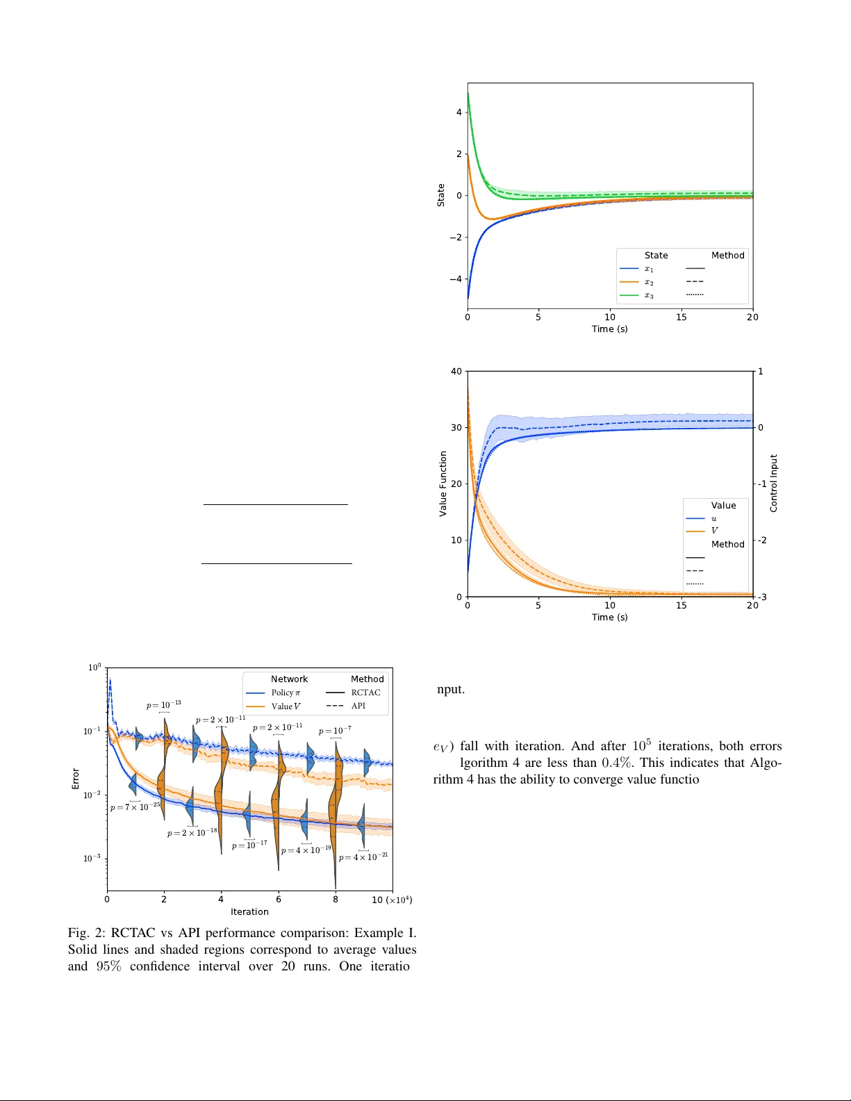
1 Relax ed Actor -Critic with Con v er gence Guarantees for Continuous-T ime Optimal Control of Nonlinear Systems Jingliang Duan, Jie Li, Qiang Ge, Shengbo Eben Li, Monimoy Bujarbaruah, Fei Ma, Dezhao Zhang ©2023 IEEE. Personal use of this material is permitted. Permission from IEEE must be obtained for all other uses, in any current or future media, including reprinting/republishing this material for advertising or promotional purposes, creating new collectiv e works, for resale or redistribution to servers or lists, or reuse of any copyrighted component of this work in other works. Abstract —This paper presents the Relaxed Continuous-Time Actor -critic (RCT A C) algorithm, a method for finding the nearly optimal policy for nonlinear continuous-time (CT) systems with known dynamics and infinite horizon, such as the path-tracking control of vehicles. RCT A C has several advantages ov er existing adaptive dynamic programming algorithms for CT systems. It does not require the “admissibility” of the initialized policy or the input-affine natur e of controlled systems f or con vergence. Instead, given any initial policy , RCT A C can conv erge to an admissible, and subsequently nearly optimal policy for a general nonlinear system with a saturated contr oller . RCT A C consists of two phases: a warm-up phase and a generalized policy iteration phase. The warm-up phase minimizes the square of the Hamiltonian to achieve admissibility , while the generalized policy iteration phase relaxes the update termination conditions for faster con vergence. The con vergence and optimality of the algorithm ar e prov en through L yapunov analysis, and its effectiveness is demonstrated through simulations and real-world path-tracking tasks. Index T erms —reinf orcement learning, continuous-time optimal control, nonlinear systems I . I N T R O D U C T I O N Dynamic Programming (DP) of fers a systematic way to solve Continuous Time (CT) infinite horizon optimal control problems with known dynamics for unconstrained linear sys- tems. It does this by using the principle of Bellman optimality and the solution of the underlying Hamilton-Jacobi-Bellman (HJB) equation [1], yielding the well-known Linear Quadratic Regulator (LQR) [2]. In this case, the optimal control policy is an affine state feedback. Howe ver , solving an infinite horizon optimal control problem analytically becomes more difficult when the system is subject to operating constraints or has nonlinear dynamics. This is because it becomes difficult to obtain an analytical solution of the HJB equation, which is Jingliang Duan and Jie Li contributed equally to this work. All correspon- dences should be sent to S. Li with email: lisb04@gmail.com. J. Duan is with the School of Mechanical Engineering, University of Science and T echnology Beijing, Beijing, 100083, China, and also with the School of V ehicle and Mobility , Tsinghua Univ ersity , Beijing, 100084, China. Email:duanjl15@163.com . J. Li, Q. Ge and S. E. Li are with the School of V ehicle and Mobility , Tsinghua University , Beijing, 100084, China. Email: jie-li18@mails.tsinghua.edu.cn, gq17@mails.tsinghua.edu.cn, lisb04@gmail.com . M. Bujarbaruah is with the Department of Mechanical Engineering, Univ ersity of California Berkeley , Berkeley , CA 94720, USA. Email: monimoyb@berkeley.edu . F . Ma is with the School of Mechanical Engineering, Univ ersity of Science and T echnology Beijing, Beijing, 100083, China. Email: yeke@ustb.edu.cn . D. Zhang is with Beijing Idriverplus T echnology Co., Ltd., Beijing, 100192, China. Email: zhangdezhao@idriverplus.com . typically a nonlinear partial differential equation [3]. This is known as the curse of dimensionality , as the computation bur - den grows exponentially with the dimensionality of the system [4]. T raditional DP methods are therefore not applicable in these cases. T o find a nearly optimal approximation of the optimal control policy for nonlinear dynamics, W erbos proposed the Adaptiv e DP (ADP) method [5], also known as Reinforcement Learning (RL) in the field of machine learning [6]–[10]. A distinct characteristic of ADP is that it utilizes a critic parameterized function, such as a Neural Network (NN), to approximate the value function, and an actor parameterized function to approximate the policy . The classical V alue Itera- tion (VI) frame work, which approximates the v alue function through one-step back-up operation, is commonly used for building ADP methods for discrete-time systems [11]. How- ev er , for CT systems, the value update law of VI requires integrating the running cost over a finite time horizon, which can lead to learning inaccuracies due to discretization error [12]. Most ADP methods adopt an iterative technique called Policy Iteration (PI) to find suitable approximations of both the value function and policy , which directly updates the v alue function by solving the corresponding L yapunov equation without the need for discretization [7]. PI consists of two- step process: 1) policy ev aluation, in which the value function mov es towards its true value associated with an admissible control policy , and 2) policy improvement, in which the policy is updated to reduce the corresponding value function. In recent years, there has been a significant amount of research on the use of ADP (or RL) techniques for the control of autonomous systems [13]–[17]. One example of CT optimal control is the ADP algorithm proposed by Ab u-Khalaf and Lewis, which seeks to find a nearly optimal constrained state- feedback controller for nonlinear systems by using a non- quadratic cost function [18]. The value function, parameterized by a linear function of hand-crafted features, is trained by the least square method at the policy ev aluation step, and the policy is e xpressed as an analytic function of the v alue func- tion. Utilizing the same single approximator scheme, Dierks and Jagannathan dev eloped a novel online parameter tuning law that ensures the optimality of both the v alue function and control policy , as well as maintaining bounded system states during the learning process [19]. [20] proposed a synchronous PI algorithm with an actor-critic framework for nonlinear CT systems without input constraints. Both the value function and policy are approximated by linear methods and tuned 2 simultaneously online. Furthermore, V amvoudakis introduced an ev ent-triggered ADP algorithm that reduces computation cost by only updating the policy when a specific condition is violated [21], and Dong et al. expanded upon this concept for use in nonlinear systems with saturated actuators [22]. In addition, ADP methods have also been widely applied in the optimal control of incompletely known dynamic systems [23]– [27] and multi-agent systems [28]–[30]. It is worth noting that most existing ADP techniques for CT systems are v alid on the basis of one or both of the follo wing two requirements: • A1: Admissibility of Initial P olicy : One is the requirement for an admissible initial polic y , meaning that the policy must be able to stabilize the system. This is because the infinite horizon value function can only be ev aluated for stabilizing control policies. Howe ver , it can be chal- lenging to obtain an admissible policy , particularly for complex systems. • A2: Input-Affine Pr operty of System : Most ADP methods are limited to input-affine systems because these methods require that the optimal policy can be represented by the value function. This means that the minimum point of the Hamilton function can be solved analytically when the value function is given. Howe ver , this is not possible for input non-af fine systems, making it difficult to directly solve the optimal policy . Note that while there are certain methods, such as integral VI [12] and parallel-control-based ADP methods [31], which do not require initial admissible control policies, they are only suitable for linear or input-affine systems. For example, the differentiation term of the time deriv ati ve of the L yapunov function with respect to the control policy can be added to its updating rule to make the initial admissible policies no longer necessary [19], [23], [32], which requires the input- affine property . [33] goes one step further and eliminates the restriction of the affine property by transforming the general nonlinear system into an affine system. Howe ver , this approach generally leads to some loss in policy performance. Additionally , the studies mentioned abov e approximate the value function or the policy using a single NN (i.e., the linear combination of predetermined hand-crafted basis functions). This means that the performance of these methods is hea vily dependent on the quality of hand-crafted features, limiting their generality since it is challenging to design such features for high-dimensional nonlinear systems. Therefore, this paper aims to address these two requirements without sacrificing optimality guarantees and generality . In this paper , we propose a relaxed continuous-time actor - critic (RCT A C) algorithm with the guarantee of con ver gence and optimality for solving optimal control problems of general nonlinear CT systems with known dynamics, which ov ercomes the limitation of the abov e two central requirements. Our main contributions are summarized as follows: 1) The warm-up phase of RCT A C is developed to relax the requirement of A1. It is proved that given any initial policy , when the activ ation function of the value network meets certain requirements, the warm-up phase can con- ver ge to an admissible policy by continuously minimizing the square of the Hamiltonian. Unlike the policy tuning rule used in [19], [23], [32], which also relaxes A1 but is restricted to input-affine systems and single-NN-based policies, the dev eloped warm-up phase is applicable to general non-af fine systems. Moreov er , RCT A C obviates the need for designing hand-crafted basis functions by utilizing multi-layer neural networks to approximate both the actor and critic, which create mappings from the system states to control inputs and the value function, respectiv ely . 2) Different from [12], [19], [23] which require input-affine systems because the policy must be represented analyt- ically by the value function, the policy network in the RCT AC algorithm is updated by directly minimizing the associated Hamiltonian using gradient descent methods in the generalized PI phase. This allows the RCT A C algorithm to be applied to arbitrary nonlinear dynamics with bounded and non-affine inputs, thereby relaxing the requirement of A2. Compared to the method of trans- forming general nonlinear systems into affine systems by creating augmented systems [33], our method does not sacrifice the guarantee of theoretical optimality . 3) W e introduce novel update termination conditions for the policy ev aluation and improvement processes, resulting in a faster conv ergence speed than the corresponding PI methods. W e also provide a L yapunov analysis to prove the con ver gence and optimality of RCT A C. Throughout the paper , we provide two detailed numerical ex- periments to sho w the generality and efficac y of the proposed RCT AC algorithm, including a linear optimal control problem and a path-tracking control task for vehicles with nonlinear and non-input-af fine dynamics. Besides, we demonstrate the practical application performance of our algorithm through an actual longitudinal and lateral vehicle control task. Organization: Section II provides the formulation of the optimal control problem and the description of PI. In Section III, we describe the RCT A C algorithm and analyze its con- ver gence and optimality . In Section IV, we present simulation examples that sho w the generality and effecti veness of the RCT AC algorithm for CT system. In Section V, we conduct experiments to verify the effecti veness of the method in practical applications. Section VI concludes this paper . I I . M AT H E M A T I C A L P R E L I M I N A R I E S A. HJB Equation This study considers the time-in variant system ˙ x ( t ) = f ( x ( t ) , u ( t )) , (1) where x ∈ R n denotes the state, u ∈ R m denotes the control input, and f : R n × R m → R n denotes the system dynamics. The dynamics f ( x, u ) is assumed to be Lipschitz continuous on a compact set Ω that contains the origin. W e suppose a continuous policy u = π ( x ) on Ω that asymptotically stabilizes the system exists. W e assume the full information of f ( x ( t ) , u ( t )) is av ailable. It can be represented by a nonlinear and input non-affine function or a Neural Network (NN) 3 only if ∂ f ( x,u ) ∂ u is accessible. The control signal u ( t ) can be saturated or unsaturated. The v alue function (cost-to-go) of policy π ( x ) is calculated as V π ( x ) = Z ∞ t l ( x ( τ ) , π ( x ( τ )))d τ    x ( t )= x , (2) where l : R n × R m → R is positiv e definite, i.e., if and only if ( x, u ) = (0 , 0) , l ( x, u ) = 0 ; otherwise, l ( x, u ) > 0 . For dynamics in (1) and the corresponding value function in (2), we giv e the associated Hamilton function H ( x, u, ∂ V π ( x ) ∂ x ) := l ( x, u ) + ∂ V π ( x ) ∂ x > f ( x, u ) . (3) Definition 1. (Admissible P olicy [34]). A contr oller π ( x ) is called the admissible policy , denoted by π ( x ) ∈ Ψ(Ω) , if it is continuous on Ω with π (0) = 0 , and stabilizes (1) on Ω . Giv en an admissible policy π ( x ) ∈ Ψ(Ω) , the differential equiv alent to (2) on Ω is called the L yapunov equation H ( x, π ( x ) , ∂ V π ( x ) ∂ x ) = 0 , (4) where V π (0) = 0 . Therefore, gi ven a policy π ( x ) ∈ Ψ(Ω) , we can obtain the value function (2) of system (1) by solving the L yapunov equation. Then the optimal control problem for Continuous T ime (CT) system can be formulated as solving a policy π ( x ) ∈ Ψ(Ω) such that the corresponding v alue function is minimum. The minimized or optimal v alue function V ? ( x ( t )) defined by V ? ( x ( t )) = min π ( x ) ∈ Ψ(Ω) Z ∞ t l ( x ( τ ) , π ( x ( τ ))d τ , (5) satisfies the classical Hamilton-Jacobi-Bellman (HJB) equa- tion min u H ( x, u, ∂ V ? ( x ) ∂ x ) = 0 , V ? (0) = 0 . (6) Meanwhile, the optimal control policy π ? ( x ) can be calcu- lated as π ? ( x ) = arg min u H ( x, u, ∂ V ? ( x ) ∂ x ) , ∀ x ∈ Ω . (7) which is the globally optimal solution to (5). Inserting V ? ( x ) and π ? ( x ) in (4), one can reformulate (6) as l ( x, π ? ( x )) + ∂ V ? ( x ) ∂ x > f ( x, π ? ( x )) = 0 with V ? (0) = 0 . The optimal value function is shown to exist and be unique in [35]. T o obtain the optimal policy , we first need to solve the HJB equation (6) to find the value function, and then use it to calculate the optimal policy using (7). Howe ver , due to the nonlinear property of the HJB equation, it is often challenging or even impossible to find a solution. B. P olicy Iteration Rather than attempting to solve the HJB equation directly , most Adaptive Dynamic Programming (ADP) methods adopt an iterativ e technique, called Policy Iteration (PI), to approx- imate both the value function and the policy [11]. PI consists of alternating between policy ev aluation using (4) and policy improv ement using (7). The algorithm proposed in this paper Algorithm 1 PI for CT optimal control Initial with policy π 0 ∈ Ψ(Ω) Giv en any small positive number  and let i = 0 while max x ∈ Ω | V i ( x ) − V i +1 ( x ) | ≥  do 1. Find value function V i ( x ) for all x ∈ Ω by l ( x, π i ( x )) + ∂ V i ( x ) ∂ x > f ( x, π i ( x )) = 0 , V i (0) = 0 (8) 2. Find new policy π i +1 ( x ) by π i +1 ( x ) = arg min u [ l ( x, u ) + ∂ V i ( x ) ∂ x > f ( x, u )] (9) i = i + 1 end while is also based on PI, as shown in the pseudocode in Algorithm 1. As shown in Algorithm 1, the first step of PI is to find an initial policy π 0 ( x ) ∈ Ψ(Ω) , because the associated value function V 0 ( x ) is finite only when the system is asymptot- ically stable. Algorithm 1 then iterati vely refines both the optimal control policy and the optimal value function. The con ver gence and optimality of the algorithm are proven in [18]. C. V alue Function and P olicy Appr oximation In previous ADP research for CT systems, the value func- tion V i ( x ) and policy π i ( x ) are usually approximated by linear methods, which requires a lar ge number of artificially designed basis functions [24]. In recent years, NNs are fa vored in many fields, such as deep learning and Reinforcement Learning (RL), due to their better generality and higher fitting ability [36]. In our work, we represent the value function and policy using multi-layer neural networks (NNs), referred to as the value NN V ( x ; ω ) ( V ω ( x ) for short) and the policy NN π ( x ; θ ) ( π θ ( x ) for short), where w and θ denote network weights. The two NNs in this case are used to map the original system states to the estimated value function and control inputs, respectiv ely . By inserting the value and polic y network in (3), we can obtain an approximated Hamiltonian expressed in terms of the parameters w and θ H ( x, ω , θ ) = l ( x, π θ ( x )) + ∂ V ω ( x ) ∂ x > f ( x, π θ ( x )) . W e refer to the algorithm combining PI and multi-layer NN as approximate PI (API), which in volves processes alternati vely tuning each of the two networks to find nearly optimal param- eters ω ? and θ ? satisfying V ω ? ( x ) ≈ V ? ( x ) , π θ ? ( x ) ≈ π ? ( x ) . Giv en any policy π θ ∈ Ψ(Ω) , the value network is tuned by solving the L yapunov equation (8) during the policy e valuation phase of API, which is equiv alent to finding parameters w to minimize the following critic loss function L c ( ω , θ ) = E x ∼ d x  H ( x, ω , θ ) 2  , (10) 4 where d x represents the state distribution ov er Ω . It is impor- tant to note that d x can be any distribution that satisfies the re- quirement of a positiv e probability density for all x ∈ Ω , such as the uniform distribution. The condition V ( x ; ω ) ≡ 0 can be easily guaranteed by selecting proper activ ation function σ V ( · ) for the v alue network. Based on (9), the policy improvement process is carried out by tuning the polic y network to minimize the expected Hamiltonian in each state, which is also called actor loss function here L a ( ω , θ ) = E x ∼ d x  H ( x, ω , θ )  . (11) The benefit of updating the policy network by minimizing L a ( ω , θ ) is that the tuning rule is applicable to any nonlinear dynamics with non-affine and constrained inputs. This relaxes the requirement of A2 (from Introduction). Since the state x is continuous, it is difficult to directly compute the expectation in (10) and (11). In practice, these two loss functions can be estimated by the sample average. W e can directly utilize existing NN optimization methods to adjust the parameters of v alue and policy NNs, such as Stochastic Gradient Descent (SGD). The value netw ork and policy network usually require multiple updating iterations to make (8) and (9) hold respectiv ely . Therefore, compared with PI algorithm, two inner updating loops w ould be introduced to update the value and policy NNs until con vergence. T aking SGD as an example, we giv e the pseudocode of API in Algorithm 2. Algorithm 2 API for CT optimal control Initial with θ 0 such that π θ 0 ( x ) ∈ Ψ(Ω) and arbitrary ω 0 Choose the appropriate learning rates α ω and α θ Giv en any small positive number  and set i = 0 while max x ∈ Ω | V ω i ( x ) − V ω i − 1 ( x ) | ≥  do 1. Estimate V ω i +1 ( x ) using π θ i ( x ) ω i +1 = ω i repeat ω i +1 = ω i +1 − α ω d L c ( ω i +1 , θ i ) d ω i +1 (12) until L c ( ω i +1 , θ i ) ≤  2. Find improved policy π θ i +1 ( x ) using V ω i +1 ( x ) θ i +1 = θ i repeat L a, old = L a ( ω i +1 , θ i +1 ) θ i +1 = θ i +1 − α θ d L a ( ω i +1 , θ i +1 ) d θ i +1 (13) until | L a ( ω i +1 , θ i +1 ) − L a, old | ≤  i = i + 1 end while I I I . R E L A X E D C O N T I N U O U S - T I M E A C T O R - C R I T I C Algorithm 2 alternately update the value and policy network by minimizing (10) and (11), respectiv ely . Note that while one NN is being adjusted, the other remains constant. Besides, each NN generally needs multiple iterations to satisfy the terminal condition, which is referred to as the protracted iterativ e computation problem [11]. This problem usually leads to the admissibility requirement because the initial policy network needs to satisfy that π ( x ; θ 0 ) ∈ Ψ(Ω) to have a finite and con ver ged value function V ( x ; ω 1 ) . Many previous studies used trials and errors process to obtain feasible initial weights for the policy network to guarantee the stability of the system [1], [21]. Ho wev er , this method usually takes a lot of time, especially for complex systems. On the other hand, the protracted problem often results in slower learning [11]. A. Description of the RCT A C Algorithm Inspired by the idea of generalized PI framew ork, which is widely utilized in discrete-time dynamic RL problems [11], we present the relaxed continuous-time actor-critic (RCT A C) algorithm for CT systems to relax the requirement A1 (from Introduction) and improve the learning speed by truncating the inner loops of Algorithm 2 without losing the con ver gence guarantees. The pseudocode of RCT AC algorithm is shown in Algorithm 3. Algorithm 3 RCT A C algorithm Initialize arbitrary θ 0 and ω 0 Choose the appropriate learning rates α , α ω and α θ Giv en any small positive number  and set i = 0 Phase 1: W arm-up while max x ∈ Ω H ( x, ω i , θ i ) ≥ 0 do Update ω and θ using: { ω i +1 , θ i +1 } = { ω i , θ i } − α d L c ( ω i , θ i ) d { ω i , θ i } (14) i = i + 1 end while Phase 2: PI with relaxed termination conditions while max x ∈ Ω | V ω i ( x ) − V ω i − 1 ( x ) | ≥  do 1. Estimate V ω i +1 ( x ) using π θ i ( x ) ω i +1 = ω i repeat Update ω i +1 using (12) until H ( x, ω i , θ i ) ≤ H ( x, ω i +1 , θ i ) ≤ 0 , ∀ x ∈ Ω 2. Find improved policy π θ i +1 ( x ) using V ω i +1 ( x ) θ i +1 = θ i repeat Update θ i +1 using (13) until max x ∈ Ω H ( x, ω i +1 , θ i +1 ) ≤ 0 i = i + 1 end while B. Con ver gence and Optimality Analysis The solution to (8) may be non-smooth for general nonlinear and input non-af fine systems. In keeping with other research in the literature [20], we make the following assumptions. Assumption 1. If π ( x ) ∈ Ψ(Ω) , its corresponding value function is smooth, i.e. V π ( x ) ∈ C 1 (Ω) (cf. [18], [20]). 5 Multiple theoretical analyses and experimental studies have demonstrated that optimization algorithms like SGD are capa- ble of locating the global minimum of the training objecti ve for multi-layer NNs in polynomial time, provided that the NN is ov er-parameterized (with a sufficiently large number of hidden neurons) [37], [38]. Based on this fact, our second assumption is: Assumption 2. Optimization algorithms like SGD can locate the global minimum of the critic loss function (10) and the actor loss function (11) for over -parameterized NNs in polynomial time. In the following section, we will demonstrate that the nearly optimal value function and policy can be obtained using Algorithm 3. T o do so, we will first introduce some necessary lemmas. Lemma 1. (Universal Appr oximation [39]). F or any con- tinuous function F ( x ) defined on a compact set Ω , it is possible to construct a feedforward NN with one hidden layer that uniformly appr oximates F ( x ) with arbitrarily small err or  ∈ R + . Lemma 1 allows us to ignore the NN approximation errors when proving the conv ergence of Algorithm 3. Lemma 2. Consider the CT dynamic optimal contr ol pr oblem for (1) and (2) . Suppose the solution ( V π ( x ) ∈ C 1 : R n → R ) of the HJB equation (6) is smooth and positive definite . The contr ol policy π ( x ) is given by (7) . Then we have that V π ( x ) = V ? ( x ) and π ( x ) = π ? ( x ) (cf. [3]). The next lemma shows ho w Algorithm 3 can be lev eraged to obtain an admissible polic y π ( x ; θ ) ∈ Ψ(Ω) gi ven any initial policy π ( x ; θ 0 ) . Lemma 3. Consider the CT dynamic optimal contr ol pr oblem for (1) and (2) . The value function (cost-to-go) V ω and policy π θ ar e repr esented by over -parameterized NNs. The parame- ters w and θ ar e initialized randomly , i.e., the initial policy π ( x ; θ 0 ) can be inadmissible. These two NNs are updated with Algorithm 3. Let Assumption 1 and 2 hold, and suppose all the hyper-par ameters (such as α , α w and α θ ) and NN optimization method ar e pr operly selected. The NN appr oximation err ors ar e ignored according to Lemma 1. Suppose all the activation functions σ V ( · ) and biases b V of the value network V ( x ; ω ) ar e set to σ V (0) = 0 and b V ( · ) ≡ 0 . At the same time, the output layer activation function σ V out also needs to satisfy σ V out ( · ) ≥ 0 . W e have that: ∃ N a ∈ Z + , if the iteration index i ≥ N a , then π ( x ; θ i ) ∈ Ψ( x ) for the system (1) on Ω . Pr oof. According to (4) and Lemma 1, there ∃ ( ω † , θ † ) , such that π ( x ; θ † ) ∈ Ψ(Ω) and H ( x, ω † , θ † ) = 0 for all x ∈ Ω , which implies that min ω ,θ L c ( ω , θ ) = min ω ,θ E x ∼ d x h H ( x, ω , θ ) 2 i = 0 . Since Algorithm 3 updates ω and θ using (14) to continu- ously minimize L c ( ω , θ ) in Phase 1, according to Assumption 2, the global minima of L c ( ω , θ ) can be obtained in poly- nomial time. Before the global minima is found, there exists N a ∈ Z + , such that H ( x, ω N a , θ N a ) ≤ 0 , ∀ x ∈ Ω . (15) T aking the time deri v ativ e of V ( x ; ω ) , we can deri ve that d V ( x ; ω ) d t = ∂ V ( x ; ω ) ∂ x > f ( x, π ( x ; θ )) , = H ( x, ω , θ ) − l ( x, π ( x ; θ )) . (16) Using (15) and (16), one has d V ( x ; ω N a ) d t ≤ − l ( x, π ( x ; θ N a )) , ∀ x ∈ Ω . As the running cost l ( x, π ( x ; θ )) is positive definite, it follows d V ω N a ( x ) d t < 0 , ∀ x ∈ Ω \{ 0 } . (17) Since σ V (0) = 0 , b V ( · ) ≡ 0 and σ V out ( · ) ≥ 0 , we have ( V ( x ; ω ) = 0 if x = 0 & ∀ ω , V ( x ; ω ) ≥ 0 if ∀ x ∈ Ω \{ 0 } & ∀ ω. (18) From (17) and (18), we have V ( x ; ω N a ) > min z ∈ Ω V ( z ; ω N a ) = 0 , ∀ x ∈ Ω \{ 0 } . (19) From (18) and (19), we infer that the value function V ( x ; ω N a ) is positi ve definite. Then, according to (17), V ( x ; ω N a ) is a L yapunov function for the closed-loop dynamics obtained from (1) when policy π ( x ; θ N a ) is used. Therefore, the policy π ( x ; θ N a ) ∈ Ψ(Ω) for the system (1) on Ω [40], that is, it is a stabilizing admissible policy . At this point, Algorithm 3 enters Phase 2. According to (4), one has min ω L c ( ω , θ N a ) = min ω E x ∼ d x h H ( x, ω , θ N a ) 2 i = 0 . So, from Assumption 2 and Lemma 1, we can always find ω N a +1 by continuously applying (12), such that H ( x, ω N a , θ N a ) ≤ H ( x, ω N a +1 , θ N a ) ≤ 0 , ∀ x ∈ Ω . Again, from Lemma 1, there always ∃ θ # , such that H ( x, ω N a +1 , θ # ) = min θ H ( x, ω N a +1 , θ ) , ∀ x ∈ Ω . Since min θ L a ( ω N a +1 , θ ) ≥ E x ∼ d x h min θ H ( x, ω N a +1 , θ ) i , we hav e L a ( ω N a +1 , θ # ) = min θ L a ( ω N a +1 , θ ) = E x ∼ d x h min θ H ( x, ω N a +1 , θ ) i . Utilizing the fact that the global minima of L a ( ω N a +1 , θ ) can be obtained, Hamiltonian H ( x, ω N a +1 , θ ) can be taken to global minimum for all x ∈ Ω by minimizing ov er θ . Then, we can also find θ N a +1 through (13), such that H ( x, ω N a +1 , θ N a +1 ) ≤ H ( x, ω N a +1 , θ N a ) ≤ 0 , ∀ x ∈ Ω . This implies that like the case with V ( x ; ω N a ) , V ( x ; ω N a +1 ) is also a L yapunov function. So, π ( x ; θ N a +1 ) ∈ Ψ(Ω) . Applying 6 this for all subsequent time steps, V ( x ; ω i ) is a L yapunov function for ∀ i ≥ N a , and it is obvious that H ( x, ω i , θ i ) ≤ H ( x, ω i +1 , θ i ) ≤ 0 , ∀ i ≥ N a & ∀ x ∈ Ω , (20) and π ( x ; θ i ) ∈ Ψ(Ω) , ∀ i ≥ N a . (21) Thus, we hav e prov ed that starting from any initial policy , the RCT AC algorithm in Algorithm 3 con ver ges to an admissible policy . As claimed previously , this relaxes the requirement A1, which is typical for most other ADP algorithms. W e now present our main result, which shows that the value NN V ( x ; ω ) and policy NN π ( x ; θ ) con verge to optimum uniformly by applying Algorithm 3. Definition 2. (Uniform Conver gence). A function sequence { f n } con ver ges uniformly to f on a set K if ∀  > 0 , ∃ N (  ) ∈ Z + , s.t. ∀ n > N , sup x ∈ K | f n ( x ) − f ( x ) | <  . Theorem 1. F or arbitrary initial value network V ( x ; ω 0 ) and policy network π ( x ; θ 0 ) , where all the activation functions σ V ( · ) and biases b V of the value network are set to σ V (0) = 0 and b V ( · ) ≡ 0 , and the output layer activation function σ V out also satisfies σ V out ( · ) ≥ 0 , if these two NNs ar e tunned with Algorithm 3, V ω i ( x ) → V ? ( x ) , π θ i ( x ) → π ? ( x ) uniformly on Ω as i → ∞ . Pr oof. From Lemma 3, it can be shown by induction that the policy π ( x ; θ i ) ∈ Ψ(Ω) for system (1) on Ω when i ≥ N a . Furthermore, according to (16) and (20), given policy π ( x ; θ i ) , we get d V ( x ; ω i ) d t ≤ d V ( x ; ω i +1 ) d t ≤ 0 , ∀ x ∈ Ω & i ≥ N a . (22) From Newton-Leibniz formula, V ω ( x ( t )) = V ω ( x ( ∞ )) − Z ∞ t d V ω ( x ( τ )) d τ d τ . (23) According to (18) and (21), V ω ( x ( ∞ )) = V ω (0) = 0 , i ≥ N a & ∀ ω . (24) So, from (18), (22), (23) and (24), we ha ve 0 ≤ V ( x ; ω i +1 ) ≤ V ( x ; ω i ) , ∀ x ∈ Ω & i ≥ N a . (25) As such, V ( x ; ω i ) is pointwise conv ergent as i goes to ∞ . One can write lim i →∞ V ( x ; ω i ) = V ( x ; ω ∞ ) . Then, the compactness of Ω directly leads to uniform con ver gence by Dini’ s theorem [41]. Next, from Definition 2, it is not hard to sho w that lim i →∞ sup x ∈ Ω | V ( x ; ω i ) − V ( x ; ω i +1 ) | = 0 . Furthermore, since V ( x ; ω i ) − V ( x ; ω i +1 ) = Z ∞ t d( V ( x ( τ ); ω i +1 ) − V ( x ( τ ); ω i )) d τ d τ , = Z ∞ t h H ( x ( τ ) , ω i +1 , θ i ) − H ( x ( τ ) , ω i , θ i ) i d τ , we hav e lim i →∞ sup x ∈ Ω | H ( x, ω i +1 , θ i ) − H ( x, ω i , θ i ) | = 0 . (26) From Lemma 1, (4) and (21), min ω L c ( ω , θ i ) = min ω E x ∼ d x h H ( x, ω , θ i ) 2 i = 0 , ∀ i ≥ N a . Since ω i +1 is obtained by minimizing L c ( ω i , θ i ) using (12), according to (26), it is true that lim i →∞ H ( x, ω i , θ i ) = lim i →∞ H ( x, ω i +1 , θ i ) = 0 , ∀ x ∈ Ω . (27) Therefore, V ( x ; ω ∞ ) is the solution of the L yapunov equation (4) when a policy π ( x ; θ ∞ ) is giv en, and it leads to that V ω ∞ ( x ) = V π θ ∞ ( x ) . The policy π ( x ; θ i ) ∈ Ψ(Ω) for i ≥ N a , so the generated state trajectory is unique due to the locally Lipschitz continuity of the dynamics [18]. Since V ( x ; ω i ) con ver ges uniformly to V ( x ; ω ∞ ) , its obvious that the system trajectory con ver ges for all x ∈ Ω . Therefore, π ( x ; θ i ) also con verges uniformly to π ( x ; θ ∞ ) on Ω . Since θ i +1 is obtained by minimizing L a ( ω i +1 , θ i ) using (13), it is obvious from (27) that lim i →∞ L a ( ω i +1 , θ i +1 ) = lim i →∞ L a ( ω i +1 , θ i ) = 0 , (28) which implies that lim i →∞ min θ H ( x, ω i , θ ) = 0 , ∀ x ∈ Ω . (29) From (27), (29), and Lemma 2, one has lim i →∞ V ( x ; ω i ) = V ? ( x ) and lim i →∞ π ( x ; θ i ) = π ? ( x ) . Therefore, one can conclude that V ω i ( x ) goes to V ? ( x ) and π θ i ( x ) goes to π ? ( x ) uniformly on Ω as i → ∞ , which means the global optimal solution is obtained. This demonstrates that the RCT AC algorithm uniformly con ver ges to the optimal value function V ? ( x ) and the optimal policy π ? ( x ) . Remark 1. The warm-up phase of RCT A C is developed to find the initial admissible policy , whose purpose is akin to that of the r elaxing initial condition of discr ete-time systems [42]. The differ ence is that the latter needs to repeatedly select an initial positive value function until the initial admissible policy can be constructed. It is pr oved that under mild r estrictions of the activation functions of the value function, given any initial pol- icy , the warm-up phase can conver ge to an admissible policy by continuously minimizing the square of the Hamiltonian. Remark 2. According to the implementation pr ocess (12) and (13) of the pr oposed RCT A C algorithm, the dynamic f ( x, u ) can be any analytic function such that ∂ f ( x,u ) ∂ u is available. As a r esult, RCT AC can be applied to any nonlinear system with non-affine and bounded contr ol inputs, unlike [12], [19], [23] which ar e only applicable to systems with affine contr ol inputs due to the requir ement for an analytical e xpr ession of the contr ol policy using the value function. Contr ol constraints can be easily incorporated by using a saturated activation function (such as tanh( · ) ) at the output of the policy network. 7 Remark 3. Since the state x is continuous, it is intr actable to chec k the value of H ( x, ω , θ ) for every x ∈ Ω . Ther efor e, in practical applications, we usually use the e xpected value of H ( x, ω , θ ) to judge whether each termination condition in Algorithm 3 is satisfied. So, the RCT A C algorithm can also be formulated as Algorithm 4. F ig. 1 shows the frameworks of API Algorithm 2 and RCT A C Algorithm 4. Algorithm 4 RCT A C algorithm: Tractable Relaxation Initialize arbitrary θ 0 and ω 0 Choose the appropriate learning rates α , α ω and α θ Giv en any small positive number  and set i = 0 Phase 1: W arm-up while L a ( ω i , θ i ) ≥  do Update ω and θ using (14) i = i + 1 end while Phase 2: PI with relaxed termination conditions while E x ∼ d x | V ω i ( x ) − V ω i − 1 ( x ) | ≥  do Update w i +1 using (12) Update θ i +1 using (13) i = i + 1 end while P ol i c y I m pr ove m e nt P ol i c y I m pr ove m e nt A PI PI 𝑉 ( 𝑥 ; 𝜔 𝑖 ) 𝜋 ( 𝑥 ; 𝜃 𝑖 ) 𝑖 = 𝑖 + 1 A d m i s s i b l e A r bi t r a r y 𝐿 𝑐 ≤ ε ∆ 𝐿 𝑎 ≤ ε 𝜔 𝑖 + 1 = 𝜔 𝑖 ∆ 𝑉 ≤ ε 𝜃 𝑖 + 1 = 𝜃 𝑖 P ol i c y E va l ua t i on 𝜋 ( 𝑥 ; 𝜃 0 ) 𝑉 ( 𝑥 ; 𝜔 0 ) V a l ue N e t w or k s t a t e 𝑉 s t a t e 𝑢 P ol i c y N e t w or k 𝑖 = 𝑖 + 1 𝜔 𝑖 + 1 = 𝜔 𝑖 𝜃 𝑖 + 1 = 𝜃 𝑖 𝑖 = 𝑖 + 1 RCTAC W a r m - up A r b i t r ar y A r bi t r a r y P ol i c y E va l ua t i on P I w i t h r e l a xe d t e r m i na t i on c ond i t i on 𝐻 ( 𝑥 , 𝜔 𝑖 , 𝜃 𝑖 ) 2 𝑉 ( 𝑥 ; 𝜔 𝑖 ) 𝜋 ( 𝑥 ; 𝜃 𝑖 ) ∆ 𝑉 ≤ ε 𝜋 ( 𝑥 ; 𝜃 0 ) 𝑉 ( 𝑥 ; 𝜔 0 ) 𝐿 𝑎 ≤ ε Fig. 1: API and RCT A C algorithm framework diagram. It is worth noting that for Algorithm 4, sometimes skipping Phase 1 and directly using Phase 2 can also obtain a nearly optimal policy . This is because even if L a ( ω i , θ i ) ≥  , Phase 2 would continuously make L a ( ω i , θ i ) approach a non-positive number by alternately using (12) to optimize V ( x ; ω ) and using (13) to optimize π ( x ; θ ) . Note that the Phase 2 of Algorithm 4 is not a CT version of the V alue Iteration (VI) method. As Lee et al. pointed out in [12], all VI methods for CT optimal control can be deemed as a v ariant of integral VI. The integral ADP methods, such as integral VI, integral PI and integral generalized PI, iterati vely perform policy ev aluation and policy improv ement updates relying on the running cost during a finite time interval [12], which is clearly different from Algorithm 3 and Algorithm 4. Besides, these integral ADP methods are usually subject to input-affine systems since these methods require that the optimal policy can be directly represented by the value function, which means that the minimum point of the Hamilton function could be solved analytically when the value function is giv en. This manner is difficult to extend to input non-af fine systems. Remark 4. In the pr evious analysis, the utility function l ( x, u ) is limited to positive definite functions, i.e., the equilibrium state (denoted by x e ) of the system must be x e = 0 . If we take x − x e as the input of value network V ( x ; ω ) , the RCT A C Algorithm 4 can be extended to pr oblems with non-zer o x e , wher e l ( x, u ) = 0 only if x = x e & u = 0 . The corresponding con ver gence and optimality analysis is similar to the pr oblem of x e = 0 . Remark 5. According to Lemma 3, all activation functions σ V and biases b V of V ( x ; ω ) ar e set to σ V (0) = 0 and b V ( · ) ≡ 0 to ensur e V ( x e ; ω ) ≡ 0 . T o remo ve these restrictions for value networks, we pr opose another effective method that drives V ( x e ; ω ) to gradually appr oach 0 by adding an equilibrium term to the critic loss function (10) L c 0 ( ω , θ ) = E x ∼ d x  H ( x, ω , θ ) 2  + η V ( x e ; ω ) 2 , wher e η balances the importance of the Hamiltonian term and the equilibrium term. I V . R E S U LT S T o verify the proposed RCT AC Algorithm 4, we of fer two numerical examples, one with linear dynamics, and the other one with a nonlinear input non-affine system (the vehicle path- tracking control). W e apply Algorithm 4 and Algorithm 2 to find the optimal solutions for these two systems. Results indicate that our algorithm outperforms Algorithm 2 in both cases. A. Example I: Linear T ime In variant System 1) Description: Consider the CT aircraft plant control problem used in [20], [21], [43], which can be formulated as min u Z ∞ 0 ( x > Qx + u > Ru )d t s . t . ˙ x =   − 1 . 01887 0 . 90506 − 0 . 00215 0 . 82225 − 1 . 07741 − 0 . 17555 0 0 − 1   x +   0 0 1   u , where Q and R are identity matrices of proper dimensions. For this linear case, the optimal analytic policy π ? ( x ) = 8 0 . 1352 x 1 + 0 . 1501 x 2 − 0 . 4329 x 3 and the optimal v alue func- tion V ? ( x ) = x > P x can be easily found by solving the algebraic Riccati equation, where P =   1 . 4245 1 . 1682 − 0 . 1352 1 . 1682 1 . 4349 − 0 . 1501 − 0 . 1352 − 0 . 1501 0 . 4329   . 2) Algorithm Details: This system is very special, in partic- ular , if the weights of the policy NN are randomly initialized around 0, which is a very common initialization method, then the initialized policy π ( x ; θ 0 ) ∈ Ψ(Ω) . Therefore, to compare the learning speed of Algorithm 2 and Algorithm 4, both algorithms are implemented to find the nearly optimal policy and value function. W e approximate the v alue function and policy using 3-layer fully-connected NNs. Each NN contains 2 hidden layers with 256 units per layer, acti vated by exponential linear units (ELUs). The outputs of the value and policy network are V ( x ; ω ) and π ( x ; θ ) , using softplus unit and linear unit as activ ation functions, respectiv ely . The training set consists of 256 states which are randomly chosen from the compact set Ω at each iteration. W e set the stepsizes α ω and α θ to 0 . 01 and employ Adam for NN optimization. 3) Result: Fig. 2 displays the learning accuracy of the policy and value function at each iteration, measured by e π = E x ∈ X 0   | π ? ( x ) − π θ ( x ) | max x ∈ X 0 π ? ( x ) − min x ∈ X 0 π ? ( x )   , e V = E x ∈ X 0   | V ? ( x ) − V ω ( x ) | max x ∈ X 0 V ? ( x ) − min x ∈ X 0 V ? ( x )   , where there are 500 states in the test set X 0 , which are ran- domly chosen from Ω . W e also draw violin plots in different iterations to show the precision distribution and 4-quartiles. 0 2 4 6 8 10 ( × 10 4 ) Iteration 10 − 3 10 − 2 10 − 1 10 0 Error [ p = 7 × 10 − 25 [ p = 2 × 10 − 18 [ p = 10 − 17 [ p = 4 × 10 − 19 [ p = 4 × 10 − 21 [ p = 10 − 13 [ p = 2 × 10 − 11 [ p = 2 × 10 − 11 [ p = 10 − 7 Network Policy π Value V Method RCTAC A PI Fig. 2: RCT A C vs API performance comparison: Example I. Solid lines and shaded re gions correspond to average v alues and 95% confidence interval over 20 runs. One iteration corresponds to one NN update. It is clear from Fig. 2 that both two algorithms can mak e the value and policy network approximation errors ( e π and 0 5 10 15 20 Time (s) 4 2 0 2 4 State State x 1 x 2 x 3 Method RCTAC A PI optimal (a) 0 5 10 15 20 Time (s) 0 10 20 30 40 Value Function Value u V Method RCTAC A PI optimal -3 -2 -1 0 1 Control Input (b) Fig. 3: Simulation results of dif ferent methods ov er 20 runs: Example I. (a) State trajectory . (b) V alue function and control input. e V ) fall with iteration. And after 10 5 iterations, both errors of Algorithm 4 are less than 0 . 4% . This indicates that Algo- rithm 4 has the ability to conv erge v alue function and policy to nearly optimal solutions. In addition, the t-test results in Fig. 2 show that both e π and e V of Algorithm 4 are significantly smaller than those of Algorithm 2 ( p < 0 . 001 ) under the same number of iterations. From the perspective of con vergence speed, Algorithm 4 requires only about 10 4 iterations to make both approximation errors less than 0.03, while Algorithm 2 requires around 10 5 steps. Based on this, Algorithm 4 is about 10 times faster than Algorithm 2. Fig. 3 shows the simulation results of the learned policy (after 10 5 iterations) ov er 20 runs. It is obvious that policies learned by RCT AC perform much better than API. The curves of state, control input, and cost generated by RCT A C are almost consistent with the optimal solution. In summary , Algorithm 4 is able to attain nearly optimal solutions and enjoys a significantly faster con vergence speed compared to 9 Algorithm 2. B. Example II: Nonlinear and Input Non-Affine System 1) Description: Consider the vehicle path tracking task with nonlinear and input non-af fine vehicle system deri ved in [44], [45]. The desired velocity is 12 m/s and the desired tracking path is shown in Fig. 5. T able I provides a detailed description of the states and inputs for this task, and T able II lists the v ehicular parameters. The vehicle’ s mov ement is controlled by a bounded actuator , where a x ∈ [ − 3 , 3] m / s 2 and δ ∈ [ − 0 . 35 , 0 . 35] rad . The dynamics of the vehicle is giv en by x =       v y r v x φ y       , u =  δ a x  , f ( x, u ) =        F y r + F y f cos δ m − v x r − bF y r + aF y f cos δ I z v y r + a x − F y f sin δ m r v y cos φ + v x sin φ        , where F y ‡ represents the lateral tire force and the subscript ‡ ∈ { f,r } corresponds to the front or rear wheels. It is calculated using the Fiala model: F y ‡ = − sgn( α ‡ ) min n | µ ‡ F z ‡ | ,      tan( α ‡ ) C ‡  1 + C 2 ‡ (tan α ‡ ) 2 27( µ ‡ F z ‡ ) 2 − C ‡ | tan α ‡ | 3 µ ‡ F z ‡       o , where F z ‡ denotes the tire load, µ ‡ denotes the lateral friction coefficient, and α ‡ denotes the tire slip angle with α f = − δ + arctan( v y + ar v x ) , α r = arctan( v y − br v x ) . The lateral friction coefficient is estimated by: µ ‡ = q ( µF z ‡ ) 2 − F 2 x ‡ F z ‡ , where F x ‡ represents the longitudinal tire force, expressed as F x f = ( 0 , a x ≥ 0 ma x 2 , a x < 0 , F x r = ( ma x , a x ≥ 0 ma x 2 , a x < 0 . The vertical loads on the front and rear wheels are approxi- mated by F z f = b a + b mg , F z r = a a + b mg . The control objectiv e is to minimize output tracking errors, which is formulated as min u Z ∞ 0 n 0 . 4( v x − 12) 2 + 80 y 2 + u >  280 0 0 0 . 3  u o d t sub ject to ˙ x = f ( x, u ) . T ABLE I: List of state and input Lateral velocity v y [m/s] Y aw rate at CG (center of gravity) r [rad/s] Heading angle between trajectory & vehicle φ [rad] Longitudinal velocity v x [m/s] Distance between trajectory & CG y [m] Front wheel angle δ [rad] Longitudinal acceleration a x [m/ s 2 ] T ABLE II: V ehicle parameters Cornering stiffness at front wheel C f -88000 [N/rad] Cornering stiffness at rear wheel C r -94000 [N/rad] Mass m 1500 [kg] Distance from front axle to CG a 1.14 [m] Distance from rear axle to CG b 1.40 [m] Polar moment of inertia of CG I z 2420 [kg · m 2 ] T ire-road friction coefficient µ 1.0 2) Algorithm Details: W e employ 6-layer fully-connected NNs to represent V ω and π θ , and the state input layer of each NN is followed by 5 fully-connected hidden layers, 32 units per layer . The activ ation function selection for the policy network is similar to that in Example I, with the exception that the output layer is activ ated by tanh( · ) with two units, multiplied by the vector [0 . 35 , 3] to accommodate the constrained control inputs. The training set consists of the current states of 256 parallel independent vehicles with different initial states, thereby obtaining a more realistic state distribution. W e use Adam method to update two NNs, while the learning rates of value network and policy network are set to 8 × 10 − 4 and 2 × 10 − 4 , respectiv ely . Besides, we use η = 0 . 1 to trade off the Hamiltonian term and the equilibrium term of the critic loss function (Remark 5). 0 2 4 6 8( × 10 4 ) Iteration 0 20 40 60 80 100 Average Absolute Hamiltonian Value | H | C Method RCTAC A PI 10 0 10 1 10 2 10 3 10 4 10 5 10 6 10 7 10 8 Finite Horizon Cost Fig. 4: RCT A C vs API performance comparison over 20 runs: Example II. 3) Result: Fig. 4 shows the ev olution of the average abso- lute Hamiltonian | H | of 256 random states and the training performance. The policy performance at each iteration is calculated by the cumulative running cost in 20s time domain C = Z 20 0 l ( x ( τ ) , u ( τ ))d τ , 10 where the initial state is randomly selected for each run. Since the initial policy is not admissible, i.e., π ( x ; θ 0 ) / ∈ Ψ(Ω) , Algorithm 2 can nev er make | H | close to 0, hence the terminal condition of policy ev aluation can nev er be satisfied. Therefore, the finite horizon cost C has no change during the entire learning process, i.e., Algorithm 2 can never conv erge to an admissible policy if π ( x ; θ 0 ) / ∈ Ψ(Ω) . On the other hand, | H | of Algorithm 4 can gradually con ver ge to 0, while the finite horizon cost C is also reduced to a small v alue during the learning process. Fig. 5 shows the control inputs and state trajectory controlled by the learned RCT AC policy . It can quickly guide the vehicle to the desired state, taking less than 0.5s for the case in Fig. 5. The results of Example II show that Algorithm 4 can solve the CT dynamic optimal control problem for general nonlinear and input non-affine CT systems with saturated actuators and handle inadmissible initial policies. 0 2 4 6 8 10 12 14 16 18 20 Time (s) 10 5 0 5 10 Control Inputs δ [ ° ] a x [ m / s 2 ] (a) 0 2 4 6 8 10 12 14 16 18 20 Time (s) 20 0 20 State v x [ m / s ] r [ ° / s ] v y [ m / s ] φ [ ° ] y [ d m ] (b) 0 100 200 300 400 Longitudinal Position (m) -3.0 -2.0 1.0 0 0.0 1.0 Lateral Position (m) Reference Trajectory Actual Trajectory (c) Fig. 5: Simulation results: Example II. (a) Control inputs. (b) State trajectory . (c) V ehicle trajectory . In conclusion, these two examples demonstrate that the proposed RCT A C method is able to learn the nearly optimal policy and value function for general nonlinear and input non- affine CT systems without reliance on initial admissible polic y . In addition, if the initial policy π ( x ; θ 0 ) ∈ Ψ(Ω) , the learning speed of Algorithm 4 is also faster than that of Algorithm 2. V . E X P E R I M E N TA L V A L I DA T I O N In this section, we demonstrate the practical ef fectiv eness of RCT AC by using the real-world path-tracking task [46], [47]. The experiment pipeline is shown in Fig. 6. The test vehicle is GEEL Y Geometry C, which is equipped with a driving mode button, enabling it to switch between manual driving mode and automatic driving mode. W e deploy the learned policy on the onboard industrial personal computer (IPC) with a 3.60 GHz Intel Core i7-7700 CPU. The deployed policy network is trained by the proposed RCT A C algorithm, where the expected velocity is set to 15 km/h, while other vehicle and algorithm parameters are consistent with Example II in Section IV -B. Provided with an ASENSING INS570D high-precision vehicle-mounted positioning system, the state of the vehicle can be accurately measured. After recei ving the vehicle state information, the IPC records and calculates control instructions ev ery 80ms, and sends the desired front wheel angle and longitudinal acceleration through the Controller Area Network (CAN), so as to realize the lateral and longitudinal control of the vehicle. s t e e r a ngl e R e a l C a r P ol i c y N e t w or k I P C s t a t e a c c e l e r a t i on Fig. 6. Real vehicle test pipeline. The control inputs and state trajectory controlled by the deployed RCT AC policy are shown in Fig. 7. From Fig. 7a, there exists a system response delay of about 0.5s between the expected and the actual control signal. Besides, the actual acceleration signals are noisy due to hardware limitations. Despite these difficulties, our policy still makes the vehicle track the desired speed and trajectory smoothly and well (Fig. 7b, 7c). For comparison, model predictive control (MPC) with a prediction time domain of 20 steps is also deployed on the IPC to carry out practical experiments [48], where the well- known nonlinear programs solver IPOPT [49] is employed to solve the constructed MPC problem. The average results of 10 independent e xperiments are sho wn in T able III. The root mean squared error (RMSE) of the heading angle between vehicle & trajectory and that of the distance between CG & trajectory φ RMSE = v u u t 1 m m X k =1 φ 2 k , y RMSE = v u u t 1 m m X k =1 y 2 k , are calculated to quantify the tracking performance. It can be found that RCT A C matches MPC in terms of tracking 11 0 2 4 6 8 10 12 14 16 20 15 10 5 0 5 F r o n t W h e e l A n g l e ( ° ) Expected A ctual 0 2 4 6 8 10 12 14 16 T ime (s) 0.5 0.0 0.5 1.0 1.5 A c c e l e r a t i o n ( m / s 2 ) Expected A ctual (a) 0 2 4 6 8 10 12 14 16 T ime (s) 10 0 10 State v x [ m / s ] e xpected velocity [m/s] r [ ° / s ] v y [ m / s ] φ [ ° ] y [ c m ] (b) 40 50 60 70 80 90 X (m) 0 10 20 Y (m) R efer ence T rajectory A ctual T rajectory (c) Fig. 7: Experiment results: (a) Control inputs. The e xpected value corresponds to the policy output. (b) State trajectory . (c) V ehicle trajectory . performance. Moreo ver , RCT A C shows great advantages in online decision-making efficiency , whose average single-step decision time is 91.17% less than that of MPC. T ABLE III: Comparison Results φ RMSE [rad] y RMSE [m] single-step decision time [ms] RCT A C 0.0797 0.0568 3.67 MPC 0.0809 0.0601 41.57 In conclusion, the vehicle experiment verifies the control effect of the proposed RCT A C algorithm in practical applica- tions. It performs as well as MPC in our path-tracking task. Moreov er , the way of offline training and online application makes the online calculation time of RCT A C much shorter than that of online optimization methods, such as MPC. This property is of significant importance for systems with limited computing resources. V I . C O N C L U S I O N The paper proposed the relaxed continuous-time actor-critic (RCT AC) Algorithm 4, along with the proof of conv ergence and optimality , for solving nearly optimal control problems of general nonlinear CT systems with known dynamics. The proposed algorithm can circumvent the requirements of “ad- missibility” and input-af fine system dynamics (described in A1 and A2 of Introduction), quintessential to previously proposed counterpart algorithms. As a result, given an arbitrary initial policy , the RCT A C algorithm is shown to eventually con ver ge to a nearly optimal policy , even for general nonlinear input non-affine system dynamics. The con ver gence and optimal- ity are mathematically prov en by using detailed L yapunov analysis. W e further demonstrate the efficacy and theoretical accuracy of our algorithm via two numerical examples, which yields a faster learning speed of the nearly optimal policy starting from an admissible initialization, as compared to the traditional approximate polic y iteration (API) algorithm (Algo- rithm 2). In addition, a real-world path-tracking experiment is conducted to verify the practical performance of our method. Results show that compared with the MPC method, RCT A C has reduced the single-step decision time by 91.17% without losing tracking performance. This indicates that our method has the potential to be applied in practical systems with limited computing resources. A P P E N D I X W e would like to ackno wledge Prof. Francesco Borrelli, Ms. Ziyu Lin, Dr . Y iwen Liao, Dr . Jiatong Xu, and Dr . Xiaojing Zhang for their valuable suggestions. R E F E R E N C E S [1] D. Liu, Q. W ei, D. W ang, X. Y ang, and H. Li, Adaptive Dynamic Pr ogramming with Applications in Optimal Contr ol . London, UK: Springer , 2017. [2] T . P appas, A. Laub, and N. Sandell, “On the numerical solution of the discrete-time algebraic riccati equation, ” IEEE T ransactions on Automatic Contr ol , vol. 25, no. 4, pp. 631–641, 1980. [3] F . L. Lewis, D. Vrabie, and V . L. Syrmos, Optimal contr ol , 3rd ed. New Y ork USA: W iley , 2012. [4] F . W ang, H. Zhang, and D. Liu, “ Adapti ve dynamic programming: An introduction, ” IEEE Computational Intelligence Magazine , vol. 4, no. 2, pp. 39–47, 2009. [5] P . W erbos, “ Approximate dynamic programming for realtime control and neural modelling, ” Handbook of Intelligent Contr ol: Neural, Fuzzy and Adaptive Approaches , pp. 493–525, 1992. [6] J. Duan, S. Eben Li, Y . Guan, Q. Sun, and B. Cheng, “Hierarchical reinforcement learning for self-driving decision-making without reliance on labelled driving data, ” IET Intelligent T ransport Systems , vol. 14, no. 5, pp. 297–305, 2020. [7] S. E. Li, Reinfor cement Learning for Sequential Decision and Optimal Contr ol . Singapore: Springer V erlag, 2023. [8] J. Duan, Y . Guan, S. E. Li, Y . Ren, Q. Sun, and B. Cheng, “Distributional soft actor-critic: Off-policy reinforcement learning for addressing value estimation errors, ” IEEE T ransactions on Neural Networks and Learning Systems , vol. 33, no. 11, pp. 6584–6598, 2021. [9] X. He, H. Y ang, Z. Hu, and C. Lv , “Robust lane change decision making for autonomous vehicles: An observation adversarial reinforcement learning approach, ” IEEE T ransactions on Intelligent V ehicles , to be published, doi: 10.1109/TIV .2022.3165178. 12 [10] Y . Li, S. He, Y . Li, L. Ge, S. Lou, and Z. Zeng, “Probabilistic charging power forecast of evcs: Reinforcement learning assisted deep learning approach, ” IEEE T ransactions on Intelligent V ehicles , to be published, doi: 10.1109/TIV .2022.3168577. [11] R. S. Sutton and A. G. Barto, Reinfor cement learning: An intr oduction . Cambridge, MA, USA: MIT Press, 2018. [12] J. Y . Lee, J. B. Park, and Y . H. Choi, “On integral v alue iteration for continuous-time linear systems, ” in American Contr ol Conference (ACC) . W ashington, DC, USA: IEEE, 2013, pp. 4215–4220. [13] K. Min, H. Kim, and K. Huh, “Deep distributional reinforcement learn- ing based high-lev el driving policy determination, ” IEEE T ransactions on Intelligent V ehicles , vol. 4, no. 3, pp. 416–424, 2019. [14] J. Duan, Z. Liu, S. E. Li, Q. Sun, Z. Jia, and B. Cheng, “ Adaptive dynamic programming for nonaffine nonlinear optimal control problem with state constraints, ” Neurocomputing , vol. 484, pp. 128–141, 2022. [15] B. Fan, Q. Y ang, X. T ang, and Y . Sun, “Rob ust ADP design for continuous-time nonlinear systems with output constraints, ” IEEE T rans- actions on Neural Networks and Learning Systems , vol. 29, no. 6, pp. 2127–2138, 2018. [16] J. Na, B. W ang, G. Li, S. Zhan, and W . He, “Nonlinear constrained optimal control of wa ve energy con verters with adaptive dynamic programming, ” IEEE T ransactions on Industrial Electr onics , vol. 66, no. 10, pp. 7904–7915, 2018. [17] J. Sun and C. Liu, “Backstepping-based adaptiv e dynamic programming for missile-target guidance systems with state and input constraints, ” Journal of the F ranklin Institute , vol. 355, no. 17, pp. 8412–8440, 2018. [18] M. Abu-Khalaf and F . L. Lewis, “Nearly optimal control laws for nonlinear systems with saturating actuators using a neural network hjb approach, ” Automatica , vol. 41, no. 5, pp. 779–791, 2005. [19] T . Dierks and S. Jagannathan, “Optimal control of affine nonlinear continuous-time systems, ” in American Control Confer ence (ACC) . Baltimore, MD, USA: IEEE, 2010, pp. 1568–1573. [20] K. G. V amvoudakis and F . L. Le wis, “Online actor critic algorithm to solve the continuous-time infinite horizon optimal control problem, ” Automatica , vol. 46, no. 5, pp. 878–888, 2010. [21] K. G. V amv oudakis, “Event-triggered optimal adaptiv e control algorithm for continuous-time nonlinear systems, ” IEEE/CAA Journal of Automat- ica Sinica , vol. 1, no. 3, pp. 282–293, 2014. [22] L. Dong, X. Zhong, C. Sun, and H. He, “Event-triggered adaptiv e dynamic programming for continuous-time systems with control con- straints, ” IEEE T ransactions on Neural Networks and Learning Systems , vol. 28, no. 8, pp. 1941–1952, 2017. [23] X. Y ang, D. Liu, and Q. W ei, “Online approximate optimal control for affine non-linear systems with unknown internal dynamics using adaptiv e dynamic programming, ” IET Contr ol Theory & Applications , vol. 8, no. 16, pp. 1676–1688, 2014. [24] Y . Jiang and Z.-P . Jiang, “Global adapti ve dynamic programming for continuous-time nonlinear systems, ” IEEE T ransactions on Automatic Contr ol , vol. 60, no. 11, pp. 2917–2929, 2015. [25] S. Xue, B. Luo, D. Liu, and Y . Li, “ Adaptive dynamic programming based ev ent-triggered control for unknown continuous-time nonlinear systems with input constraints, ” Neur ocomputing , vol. 396, pp. 191– 200, 2020. [26] H. Jiang and B. Zhou, “Bias-policy iteration based adapti ve dynamic programming for unknown continuous-time linear systems, ” A utomatica , vol. 136, pp. 1–12, 2022. [27] N. W ang, Y . Gao, H. Zhao, and C. K. Ahn, “Reinforcement learning- based optimal tracking control of an unknown unmanned surface ve- hicle, ” IEEE T ransactions on Neural Networks and Learning Systems , vol. 32, no. 7, pp. 3034–3045, 2020. [28] K. G. V amvoudakis, F . L. Lewis, and G. R. Hudas, “Multi-agent differential graphical games: Online adaptiv e learning solution for syn- chronization with optimality , ” Automatica , v ol. 48, no. 8, pp. 1598–1611, 2012. [29] J. Li, H. Modares, T . Chai, F . L. Lewis, and L. Xie, “Off-policy rein- forcement learning for synchronization in multiagent graphical games, ” IEEE T ransactions on Neural Networks and Learning Systems , vol. 28, no. 10, pp. 2434–2445, 2017. [30] J. Shi, D. Y ue, and X. Xie, “Data-based optimal coordination control of continuous-time nonlinear multi-agent systems via adaptive dynamic programming method, ” J ournal of the F ranklin Institute , v ol. 357, no. 15, pp. 10 312–10 328, 2020. [31] J. Lu, Q. W ei, T . Zhou, Z. W ang, and F .-Y . W ang, “Event-triggered near-optimal control for unknown discrete-time nonlinear systems using parallel control, ” IEEE Tr ansactions on Cybernetics , 2022. [32] X. Y ang, Z. Zeng, and Z. Gao, “Decentralized neurocontroller design with critic learning for nonlinear-interconnected systems, ” IEEE T ransactions on Cybernetics , to be published, doi: 10.1109/TCYB.2021.3085883. [33] J. Lu, Q. W ei, and F .-Y . W ang, “Parallel control for optimal tracking via adaptive dynamic programming, ” IEEE/CAA Journal of Automatica Sinica , vol. 7, no. 6, pp. 1662–1674, 2020. [34] R. W . Beard, G. N. Saridis, and J. T . W en, “Galerkin approximations of the generalized Hamilton-Jacobi-Bellman equation, ” Automatica , vol. 33, no. 12, pp. 2159–2177, 1997. [35] S. L yashevskiy , “Constrained optimization and control of nonlinear systems: new results in optimal control, ” in Proceedings of 35th IEEE Confer ence on Decision and Control (CDC) . Kobe, Japan: IEEE, 1996, pp. 541–546. [36] Y . LeCun, Y . Bengio, and G. E. Hinton, “Deep learning, ” Nature , vol. 521, pp. 436–444, 2015. [37] Z. Allen-Zhu, Y . Li, and Z. Song, “ A conv ergence theory for deep learn- ing via over-parameterization, ” in Pr oceedings of the 36th International Confer ence on Machine Learning (ICML) . Long Beach, CA, USA: PMLR, 2019, pp. 242–252. [38] S. Du, J. Lee, H. Li, L. W ang, and X. Zhai, “Gradient descent finds global minima of deep neural networks, ” in Pr oceedings of the 36th International Conference on Machine Learning (ICML) . Long Beach, CA, USA: PMLR, 2019, pp. 1675–1685. [39] K. Hornik, M. Stinchcombe, and H. White, “Univ ersal approximation of an unknown mapping and its derivati ves using multilayer feedforward networks, ” Neural Networks , vol. 3, no. 5, pp. 551–560, 1990. [40] A. M. L yapunov , “The general problem of the stability of motion, ” International Journal of Control , vol. 55, no. 3, pp. 531–534, 1993. [41] R. G. Bartle and D. R. Sherbert, Introduction to real analysis , 3rd ed. New Y ork, NY , USA: Wile y , 2000. [42] D. Liu, Q. W ei, and P . Y an, “Generalized policy iteration adaptive dy- namic programming for discrete-time nonlinear systems, ” IEEE T rans- actions on Systems, Man, and Cybernetics: Systems , vol. 45, no. 12, pp. 1577–1591, 2015. [43] B. L. Stev ens and F . L. Lewis, Air craft contr ol and simulation . New Y ork, NY , USA: W iley , 2004. [44] J. Kong, M. Pfeiffer , G. Schildbach, and F . Borrelli, “Kinematic and dynamic v ehicle models for autonomous dri ving control design, ” in IEEE Intelligent V ehicles Symposium (IV) . Seoul, South Korea: IEEE, 2015, pp. 1094–1099. [45] R. Li, Y . Li, S. Li, E. Burdet, and B. Cheng, “Driver-automation indirect shared control of highly automated v ehicles with intention-a ware authority transition, ” in IEEE Intelligent V ehicles Symposium (IV) . Los Angeles, CA, USA: IEEE, 2017, pp. 26–32. [46] L. Li, W .-L. Huang, Y . Liu, N.-N. Zheng, and F .-Y . W ang, “Intelligence testing for autonomous vehicles: A new approach, ” IEEE T ransactions on Intelligent V ehicles , vol. 1, no. 2, pp. 158–166, 2016. [47] S. Ge, F .-Y . W ang, J. Y ang, Z. Ding, X. W ang, Y . Li, S. T eng, Z. Liu, Y . Ai, and L. Chen, “Making standards for smart mining operations: Intelligent vehicles for autonomous mining transportation, ” IEEE T ransactions on Intelligent V ehicles , vol. 7, no. 3, pp. 413–416, 2022. [48] Y . Lin, J. McPhee, and N. L. Azad, “Comparison of deep reinforcement learning and model predictive control for adaptive cruise control, ” IEEE T ransactions on Intelligent V ehicles , vol. 6, no. 2, pp. 221–231, 2021. [49] A. W achter and L. T . Biegler , “Biegler , l.t.: On the implementation of a primal-dual interior point filter line search algorithm for large- scale nonlinear programming. mathematical programming 106, 25-57, ” Mathematical Progr amming , vol. 106, no. 1, pp. 25–57, 2006.