Set-based MPC for discrete-time LTI systems with maximal domain of attraction and minimal predictive control horizon

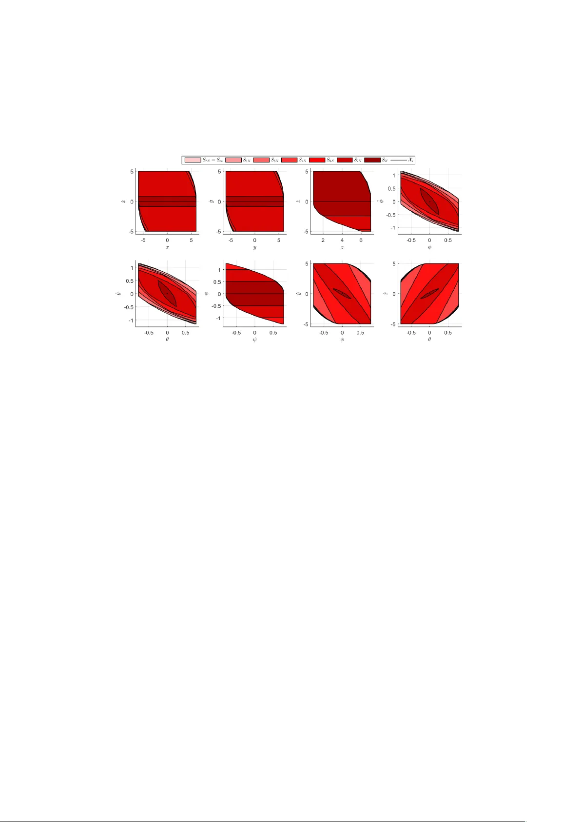
Set-based MPC for discrete-time L TI systems with maximal domain of attraction and minimal predictiv e control horizon Alejandro Anderson a , Agustina D’Jorge a , Alejandro H. Gonz ´ alez a , Antonio Ferramosca b , Marcelo Actis c a Institute of T echnological Dev elopment for the Chemical Industry (INTEC), CONICET - Univ ersidad Nacional del Litoral (UNL). G ¨ uemes 3450, (3000) Santa Fe, Argentina. b Department of Management, Information and Production Engineering, Univ ersity of Bergamo. V ia Marconi 5, 24044 Dalmine (BG), Italy . c Facultad de Ingenier ´ ı a Qu ´ ı mica, UNL-CONICET , Santiago del Estero 2829, (3000) Santa Fe, Argentina. Corresponding A uthor: Marcelo Actis Facultad de Ingenier ´ ı a Qu ´ ı mica, UNL–CONICET —– Postal Address: FIQ, UNL, Santa Fe Santiago del Estero 2829. S3000A OM, Santa Fe, ARGENTINA. —– Phone: +54 342 4580 3164 e-mail: mactis@ fi q.unl.edu.ar Set-based MPC for discrete-time L TI systems with maximal domain of attraction and minimal predictiv e control horizon Abstract This paper presents a nov el set-based model predictiv e control for tracking, which pro- vides the largest domain of attraction, e ven with the minimal predictive/control hori- zon. The formulation - which consists of a single optimization problem - shows a dual behavior: one operating inside the maximal controllable set to the feasible equi- librium set, and the other operating at the N -controllable set to the same equilibrium set. Based on some fi nite-time conv ergence results, asymptotic stability of the result- ing closed-loop is proved, while recursi ve feasibility is ensured for any change of the setpoint. The properties and advantages of the proposal have been tested on simulation models. K e ywor ds: Set-based MPC, Domain of Attraction, Recursiv e feasibility , Asymptotic stability , MPC for T racking. 1. Introduction Model Predictiv e Control (MPC) is a strategy widely used in industries since the 1980s, due to its ability to deal with multi variable processes including both, state and input constraints. A strong theoretical framew ork has been developed in the last two decades, showing that MPC is a control technique capable to guarantee asymptotic stability , constraint satisfaction and robustness, based on the solution of an on-line tractable optimization problem for both, linear and nonlinear systems. L yapunov theory provides a general framework to prove asymptotic stability of a system controlled by an MPC, by employing suitable terminal ingredients (terminal cost, terminal equality or inequality constraint) ([10, 23, 22]). The stabilizing terminal constraint implicitly imposes hard restrictions on the state, since only those states that can be steered in a given number of steps to the terminal region will be properly stabilized. These states determine the so-called closed-loop domain of attraction, whose characterization is crucial because it represents a domain of validity that is determined not just by the system dynamic and its constraints, but also by the speci fi c controller design. In this context, any effort to modify the classical MPC formulation to have a larger domain of attraction is remarkably bene fi cial, as it was stated in many seminal works ([16, 19]). The most obvious way to enlarge the MPC domain of attraction is by enlarging the prediction/control horizon. Howe ver , this strategy has two major drawbacks. Firstly , it produces a signi fi cant increase of the computational burden. Secondly , it is not unusual Pr eprint submitted to XX F ebruary 16, 2023 that during the operation of the plant the desired setpoint where the system has to be stabilized may change. As a result, the stabilizing terminal ingredients may become in v alid, the feasibility of the MPC optimization problem may be lost, and the controller may fail to track the desired setpoint. T o solve the loss of feasibility under setpoint changes, different solutions ha ve be- ing proposed in the literature, such as r efer ence governors MPC ([25, 5]) and MPC for T racking (MPCT) ([20, 8, 18, 21]). This latter strategy solves the problem of recursive feasibility by penalizing the distance from the predicted trajectories to some extra arti- fi cial optimization v ariables, which are forced to be a feasible equilibrium. This way , not only the recursi ve feasibility is ensured for any change of setpoints, but also the domain of attraction is enlarged (although it does not necessarily reach the maximal domain of attraction, for a giv en prediction horizon), since it results to be the N-step controllable set to any equilibrium point of the system to be controlled, and not just the a speci fi c one. Another approach, tending to enlarge the MPC domain of attraction in a rather the- oretical form, was presented in [19]. The idea was to substitutes the terminal constraint by a kind of contractiv e terminal constraint, which forces the terminal state to pass from one control in variant set to another . The proposed method reaches the maximal domain of attraction (the so-called maximal contr ollable set to the equilibrium , which is determined by the system and the constraints), but the computation of the control in v ariant sets, which may be computationally prohibitiv e, must be carried out on line ev ery time a change in the setpoint occurs. In this work we propose a novel MPC design based on set-based predictiv e con- trol. In contrast to regular MPC in the so-called set dynamical systems framework ([6, 24]), the state of a system is identi fi ed by a set rather than a point. The set-based predictiv e controller generalizes conv entional MPC along the lines of the tube based MPC approach [4, 9]. In particular , [4] is devoted to obtain provably safe controllers for disturbed nonlinear systems with constraints on states and inputs, while in [9] a reachable-set based version of the robust MPC based on tightened constraints originally proposed in [7] is presented. Some approaches use reachable sets based on zonotopes [12] to compute the reachable sets. Howev er , it is worth to mention that the referred set-based strategies are not in the same control framework as the proposal. The aim of this work is to extend the domain of attraction up to the maximal controllable set for any fi xed prediction horizon – even the minimum possible horizon – without loss of feasibility under changes of the setpoint. The method consists in a decomposition of the maximal domain of attraction into a disjoint union of embedded layers de fi ned by the controllable sets of the system. The proposed controller shows a dual beha vior , but into an uni fi ed formulation. First, the goal of the controller is to driv e the system through the layers until a proper neighborhood of the equilibrium set is reached. This neighborhood is actually the domain of attraction of the classical MPCT [20]. Once the state of the system is inside this set, analogously to the classical MPCT , the asymptotic stability of (any point in) the equilibrium set is guaranteed. This paper is organized as follows. W e set up our notation in Section 1.1. In Sec- tion 2 we present general de fi nitions and necessaries results to formulate the proposed MPC. For the sake of completeness we include in Section 2.1 a brief recall of the MPCT . Section 3 is dev oted to describe in detail the proposed controller . The proof 2 of the main results are addressed in Section 3.1. Finally , numerical simulations and conclusions can be found in Section 4 and 5, respectiv ely . 1.1. Notation W e denote with N the sets of integers, N 0 := N ∪ { 0 } and I i := { 0 , 1 , . . . , i } . The euclidean distance between two points x, y ∈ R d by � x − y � := [( x − y ) � ( x − y )] 1 / 2 , where x � denotes the transpose of x . If P is a positiv e-de fi nite matrix on R d × d then we de fi ne the quadratic form � x − y � 2 P := ( x − y ) � P ( x − y ) . Let X ⊆ R d . The open ball with center in x ∈ X and radius ε > 0 r elative to X is giv en by B X ( x, ε ) := { y ∈ X : � x − y � < ε } . Giv en x ∈ Ω ⊆ X , we say that x is an interior point of Ω r elative to X if the there exist ε > 0 such that the open ball B X ( x, ε ) ⊆ Ω . The interior of Ω relative to X is the set of all interior points and it is denoted by int X Ω . In case X = R d we omit the subscript in the latter de fi nition, i.e. int Ω := int R d Ω . Finally , let Ω 1 and Ω 2 two sets in R d , we denote the dif ference between Ω 1 and Ω 2 by Ω 1 \ Ω 2 := { x ∈ Ω 1 : x / ∈ Ω 2 } . 2. Problem statement and preliminaries Consider a system described by a linear discrete-time in v ariant model x ( i + 1) = Ax ( i ) + B u ( i ) (2.1) where x ( i ) ∈ X ⊂ R n is the system state at time i and u ( i ) ∈ U ⊂ R m is the current control at time i , where X and U are compact con vex sets containing the origin. As usual, the plant model is assumed to ful fi ll the following assumption: Assumption 2.1. The pair ( A, B ) is contr ollable and the state is measur ed at each sampling time. The set of steady states and inputs of the system (2.1) is giv en by Z s := { ( x s , u s ) ∈ X × U : x s = Ax s + B u s } . Thus, the equilibrium state and input sets are de fi ned as X s := pro j X Z s and U s := pro j U Z s . The goal of this work is to propose a set based MPC which ensures at the same time maximal domain of attraction and feasibility/asymptotic stability under any change of setpoint. T o this aim, let us fi rst introduce the de fi nitions of the main sets necessary for the formulation of the MPC proposed in Section 3. De fi nition 2.2 (Control In variant Set). A set Ω ⊂ X is a Contr ol Invariant Set (CIS) of system (2.1) if for all x ∈ Ω , there exists u ∈ U such that Ax + B u ∈ Ω . Associated to Ω is the corr esponding input set Ψ ( Ω ) := { u ∈ U : ∃ x ∈ Ω such that Ax + B u ∈ Ω } . 3 De fi nition 2.3 ( i -Step Controllable Set). Given i ∈ N and two sets Ω ⊆ X and Ψ ⊆ U , the i-step controllable set to Ω corresponding to the input set Ψ , of system (2.1) , is given by S i ( Ω , Ψ ) := { x 0 ∈ X : ∀ j ∈ I i − 1 , ∃ u j ∈ Ψ such that x j +1 = Ax j + B u j ∈ X and x i ∈ Ω } . F or con venience, we de fi ne S 0 ( Ω , Ψ ) := Ω and S ∞ ( Ω , Ψ ) :=  ∞ i =0 S i ( Ω , Ψ ) , i.e. the set of admissible states which can be steered to the set Ω by a fi nite sequence of inputs in Ψ ⊆ U . According to the latter de fi nition, the maximal domain of attraction that the con- strained system allows, for any setpoint x ∗ in the equilibrium set X s , is giv en by S ∞ ( X s , U ) . Next, we de fi ne a new special type of in v ariant sets, which are a key concept of this work. De fi nition 2.4 (Contractive CIS). Let Ω ⊂ S ∞ := S ∞ ( Ω , U ) be a CIS. Then Ω is a contractive CIS if for all x ∈ Ω , there exists u ∈ U such that Ax + B u ∈ int S ∞ Ω . Note that the above de fi nition is similar to the de fi nition of a γ -Contr ol Invariant Set 1 (see [6]). Indeed, if Ω is a γ -control inv ariant set then for all x ∈ Ω , there exists u ∈ U such that Ax + B u ∈ in t Ω ⊆ in t S ∞ Ω . Hence ev ery γ -control inv ariant set is a contractiv e CIS. Ho wev er the in verse result is not necessary true. For instance, it can be shown that the sets S kN corresponding to the double integrator presented in Section 4 are Contractiv e CIS but, due to the fact that they share some part of the boundary (see Figure 3), it cannot be ensured that they are γ -CIS. The importance of considering the weakened concept of interior relative to the set S ∞ will be addressed in Remark 2.7. Lemma 2.5 (Geometric property of contractive CIS). Let Ω ⊂ S ∞ be a compact and con vex contractive CIS of system (2.1) . Then, Ω ⊆ in t S ∞ S 1 ( Ω , Ψ ( Ω )) . Pr oof. It is easy to see that Ω ⊆ S 1 ( Ω , Ψ ( Ω )) by the in variance property of the set. It remains to show that ev ery point of Ω is an interior point of S 1 ( Ω , Ψ ( Ω )) relative to S ∞ . Let x ∈ Ω , since Ω is a contracti ve CIS, there exists u ∈ Ψ ( Ω ) such that Ax + B u ∈ int S ∞ Ω . Then, there exists ε > 0 such that B S ∞ ( Ax + B u, ε ) ⊆ Ω . Since Ax + B u is a continuous function at x from S ∞ to S ∞ , then there exists δ > 0 such that for all ˜ x ∈ B S ∞ ( x, δ ) we hav e A ˜ x + B u ∈ B S ∞ ( Ax + B u, ε ) ⊆ Ω . Hence ˜ x ∈ S 1 ( Ω , Ψ ( Ω )) . Therefore B S ∞ ( x, δ ) ⊆ S 1 ( Ω , Ψ ( Ω )) , that is to say so Ω ⊆ int S ∞ ( S 1 ( Ω , Ψ ( Ω ))) . 1 Ω is a γ -Control In variant Set ( γ -CIS) if for x ∈ Ω there exists u ∈ U such that Ax + B u ∈ γ Ω , for some γ < 1 . 4 The next lemma sho ws that the contractive in variance property is inheritable for the controllable sets. Lemma 2.6. Let Ω ⊂ X be a compact and con vex contractive CIS of system (2.1) . Then for every i ∈ N , the set S i ( Ω , U ) is a con ve x and compact contractive CIS of system (2.1) . Pr oof. Since Ω is under the assumptions of Lemma 2.5 and Ψ ( Ω ) ⊆ U then Ω ⊆ int S ∞ S 1 ( Ω , Ψ ( Ω )) ⊆ in t S ∞ S 1 ( Ω , U ) . Hence S 1 ( Ω , U ) is a contracti ve CIS of system (2.1). By [15] we know that S 1 ( Ω , U ) is compact and con vex. Therefore S 1 ( Ω , U ) is also under the assumptions of Lemma 2.5. The result follows by induction. Remark 2.7. Observe that in Lemma 2.5 we pr ove a geometric pr operty of the con- tractive CIS analogous to Pr operty 1 in [3] for γ -CIS. However in [3] it is r equir ed that Ω ⊆ in t X . This r equir ement r epr esents an obstacle in the proof of Lemma 2.6 when we apply recur sively Lemma 2.5 to the sets S i ( Ω , U ) . Notice that, for i lar ge enough, the sets S i ( Ω , U ) usually collapse in the boundary of X (see F igur e 3). Therefor e they will not ful fi ll the hypothesis S i ( Ω , U ) ⊆ int X . Next, we de fi ne a class of sets constituting a nested disjoint decomposition of the state space. De fi nition 2.8 ( k -Lay er Set). Let Ω ⊂ X be a contr ol invariant set, Ψ ⊆ U an in- put set and N ∈ N . F or any k ∈ N 0 we de fi ne the k -Layer Set by L kN ( Ω , Ψ ) := S ( k +1) N ( Ω , Ψ ) \ S kN ( Ω , Ψ ) . Remark 2.9. In the above de fi nition we ask for Ω to be an in variant set. This implies that the i -Step Contr ollable Sets S i ( Ω , Ψ ) , i ∈ N 0 , ar e nested (see Lemma 1 in [19]). Hence the k -Layer Sets ar e disjoint (see F igur e 1) and even mor e S ∞ ( Ω , Ψ ) = S N ( Ω , Ψ ) ∪ ∞  k =1 L kN ( Ω , Ψ ) . (2.2) 5 Figure 1: The fi rst fi v e layers for the harmonic oscillator system. 2.1. MPC for T racking (MPCT) The MPC for tracking ([21]) attempts to track any admissible target steady sate by means of admissible e volutions, with an arti fi cial reachable setpoint in X s added as decision variable. The MPCT cost function has two terms. The fi rst one is a quadratic cost of the expected tracking error with respect to the arti fi cial steady state and input ( x s , u s ) . The second one is the offset cost function V O ( x s , x ∗ ) , that penalizes the deviation from the arti fi cial steady state x s to the desired setpoint x ∗ . The MPCT cost function is given by V N ( x, x ∗ ; u , x s , u s ) = N − 1  j =0 � x j − x s � 2 Q + � u j − u s � 2 R + V O ( x s , x ∗ ) , (2.3) where N is the control horizon, u is a sequence of N future control inputs, i.e. u = { u 0 , · · · , u N − 1 } , x j is the predicted state of the system at time j giv en by x j +1 = Ax j + B u j , with x 0 = x . The offset cost function is required to be a conv ex and positiv e-de fi nite function (see [21]). For simplicity , in this work we will considered it as a quadratic function V O ( x s , x ∗ ) = � x s − x ∗ � 2 T , being T a positiv e-de fi nite matrix. If a terminal equality constraint is used to ensure stability , the MPCT optimization problem P T N ( x, x ∗ ) is giv en by min u ,x s ,u s V N ( x, x ∗ ; u , x s , u s ) (2.4) 6 s.t. x 0 = x, (2.5) x j +1 = Ax j + B u j , j ∈ I N − 1 , (2.6) x j ∈ X , u j ∈ U , j ∈ I N − 1 , (2.7) ( x s , u s ) ∈ Z s , (2.8) x N = x s . (2.9) Constraint (2.8) ensures that the arti fi cial v ariable ( x s , u s ) is an admissible equilibrium point. The terminal equality constraint (2.9) forces the terminal state to be the arti fi - cial state, that is to be the best (based on the offset cost function) admissible equilib- rium point. These constraints ensure recursiv e feasibility and stability of the resulting closed-loop, for any state in S N ( X s , U ) 2 , avoiding the loss of feasibility in presence of changes in the setpoint. 3. The proposed MPC For a fi xed control horizon N ∈ N , we are going to present a novel stable MPC for tracking that provides, for any setpoint in the equilibrium set, x ∗ ∈ X s , the maximal domain of attraction, i.e., the maximal controllable set S ∞ . From now on, we simplify the notation by denoting S i := S i ( X s , U ) and L i := L i ( X s , U ) . Let x ∈ S ∞ . The following cost function is proposed V N ( x ; u , x a , u a , x s ) = N − 1  j =0 � x j − x a j � 2 Q + � u j − u a j � 2 R + V O ( x s , x ∗ ) , (3.1) where, as before, u := { u 0 , · · · , u N − 1 } represents a sequence of N future control inputs and x j is the predicted state of the system at time j giv en by x j +1 = Ax j + B u j , with x 0 = x . The sequence of N state and control auxiliary v ariables x a := { x a 0 , · · · , x a N − 1 } and u a := { u a 0 , · · · , u a N − 1 } , hav e the purpose of accounting for the distance of the states x j and inputs u j to some sets that we will de fi ne later . Finally , x s represents an arti fi cial variable in X s and V O ( x s , x ∗ ) = � x s − x ∗ � 2 T . The controller is deri ved from the solution of the optimization problem P N ( x, x ∗ ) giv en by min u , x a , u a ,x s V N ( x ; u , x a , u a , x s ) (3.2) s.t. x 0 = x, (3.3) x j +1 = Ax j + B u j , (3.4) 2 In the traditional MPC the domain of attraction is S N ( x ∗ , U ) , which is signi fi cantly smaller than S N ( X s , U ) . 7 x j ∈ X , j ∈ I N − 1 , (3.5) u j ∈ U , j ∈ I N − 1 , (3.6) x a j ∈ Ω x , j ∈ I N − 1 , (3.7) u a j ∈ Ψ ( Ω x ) , j ∈ I N − 1 , (3.8) x N ∈ Ω x , (3.9) x s ∈ X s , (3.10) where Ω x is a target set that depends on the initial state x , and it is de fi ned as Ω x =  S kN , x ∈ L kN , with k ≥ 1 { x s } , x ∈ S N , (3.11) and the set Ψ ( Ω x ) is the corresponding input set to Ω x . Note that when the state of the system is inside S N we have that Ω x = { x s } , therefore the corresponding input set is Ψ ( Ω x ) = { u s } , with u s such that x s = Ax s + B u s . Considering the receding horizon policy , the control law is given by κ M P C ( x ) = o u 0 , where o u 0 is the fi rst element of the optimal input sequence o u = { o u 0 , · · · , o u N − 1 } . The optimal cost is de fi ned by o V N ( x ) := V N ( x ; o u , o x a , o u a , o x s ) where o u , o x a , o u a , o x s are the optimal solutions to Problem P N ( x, x ∗ ) . Remark 3.1. The formulation of pr oblem P N ( x, x ∗ ) depends on the computation of the contr ollable sets S kN , for all k ∈ N . Since X is a compact set, the sequence S k con ver ges (up to a given tolerance) in fi nite steps to the set S ∞ . So the number of sets to be computed is fi nite. On the other hand, these contr ollable sets depend only on the entir e equilibrium set X s and not on a speci fi c setpoint x ∗ , i.e. the y remain the same r e gar dless of any chang e on the setpoint. Therefor e these sets can be computed off-line, which signi fi cantly simpli fi es the implementation of the optimization pr oblem. This is the main advantage of the pr oposed approac h with r espect to the one pr esented in [19]. It is easy to see that Problem P N ( x, x ∗ ) presents a dual behaviour just replacing the set Ω x on equations (3.7)–(3.9) according to (3.11) and the position of the initial state. W e summarized explicitly this dual behaviour in the following properties. Property 3.2. When the curr ent state x belongs to S ∞ \ S N , ther e e xists k ≥ 1 such that x ∈ L kN , and the arti fi cial variable x s does not depend on any other optimization variable. Ther efor e, by optimality , it will be equal to x ∗ ∈ X s and � x s − x ∗ � = 0 . Hence the pr oblem to be solved is equivalent to min u N − 1  j =0 d Q ( x j , Ω x ) + d R ( u j , Ψ ( Ω x )) (3.12) s.t. x 0 = x, x j +1 = Ax j + B u j , j ∈ I N − 1 , 8 x j ∈ X , j ∈ I N − 1 , u j ∈ U , j ∈ I N − 1 , x N ∈ Ω x , wher e Ω x = S kN , d Q ( x j , Ω x ) := min { � x j − x a j � 2 Q : x a j ∈ Ω x } is a distance fr om the pr edicted state x j to the tar get set Ω x and d R ( u j , Ψ ( Ω x )) := min { � u j − u a j � 2 R : u a j ∈ Ψ ( Ω x ) } is a distance fr om the contr ol u j to the set Ψ ( Ω x ) . In other wor ds, while the curr ent state does not r each S N , the contr oller tries to minimize the distance of the pr edicted trajectory to the next layer . Property 3.3. When the contr olled system reac hes S N , the targ et set is Ω x = { x s } . Then by constraint (3.9) x N = x s , by (3.7) x a 0 = x a 1 = · · · = x a N − 1 = x s , and by (3.8) u a 0 = u a 1 = · · · = u a N − 1 = u s , with u s such that x s = Ax s + B u s . So the MPCT described in Section 2.1 is r ecover ed. 3.1. Asymptotic stability: preliminaries From now on we consider the following assumption. Assumption 3.4. The set S N is a contractive CIS. Remark 3.5. Note that the above assumption is not so r estrictive. F or example it is suf fi cient to have S N − 1 ⊆ int S ∞ S N , even when it is not true that S N − 1 ⊆ int S N (see Figur e 3). Indeed, if S N − 1 ⊆ int S ∞ S N then S N is a contractive CIS, and by Lemma 2.6 all S kN ar e also contractive CIS, for any k ≥ 1 . First of all note that the recursiv e feasibility is an immediate consequence of the nested property of the controllable sets S i . Howe ver , the proof of attractivity is more subtle since the optimal cost is not a L yapunov function in the entire domain of at- traction. In order to prov e that the real trajectory produced by the proposed strategy reaches the set S N in a fi nite number of steps, we need fi rst to suppose the opposite, i.e, we need to proceed by contradiction. The following lemma goes in this direction. Lemma 3.6. Let x ∈ L kN for some k ≥ 1 . Let { x ( i ) } ∞ i =0 be the sequence given by the closed-loop system x ( i + 1) = Ax ( i ) + B κ M P C ( x ( i )) , with x (0) = x . If x ( i ) / ∈ S kN for all i ∈ N then d Q ( x ( i ) , S kN ) → 0 when i → ∞ . Pr oof. Suppose the solution of Problem P N ( x ( i ) , x ∗ ) is giv en by o u = { o u 0 , . . . , o u N − 1 } , o u a = { o u a 0 , . . . , o u a N − 1 } , o x a = { o x a 0 , . . . , o x a N − 1 } , o x s = x ∗ and the corresponding opti- mal state sequence is giv en by o x = { o x 0 , . . . , o x N } , where o x 0 = x ( i ) and o x N ∈ S kN . The optimal cost is giv en by o V N ( x ( i )) = N − 1  j =0 � o x j − o x a j � 2 Q + � o u j − o u a j � 2 R . Since S kN is an inv ariant set, then there exists ˆ u ∈ Ψ ( S kN ) such that ˆ x = A o x N + B ˆ u ∈ S kN . Then a feasible solution to problem P N ( x ( i + 1) , x ∗ ) is ˆ u = { o u 1 , . . . , o u N − 1 , ˆ u } , 9 ˆ u a = { o u a 1 , . . . , o u a N − 1 , ˆ u } , ˆ x a = { o x a 1 , . . . , o x a N − 1 , o x N } and ˆ x s = x ∗ . The state se- quence associated to the feasible input sequence ˆ u is given by ˆ x = { o x 1 , . . . , o x N , ˆ x } . Since o x 1 = x ( i + 1) / ∈ S kN then it is easy to see that o x 1 ∈ L kN 3 . Therefore the feasible cost corresponding to ˆ u , ˆ u a , ˆ x a and ˆ x s , is giv en by V N ( x ( i + 1); ˆ u , ˆ x a , ˆ u a , ˆ x s ) = N − 1  j =1  � o x j − o x a j � 2 Q + � o u j − o u a j � 2 R  + � o x N − o x N � 2 Q + � ˆ u − ˆ u � 2 R    =0 , which means that V N ( x ( i + 1); ˆ u , ˆ x a , ˆ u a , ˆ x s ) − o V N ( x ( i )) = −� o x 0 − o x a 0 � 2 Q − � o u 0 − o u a 0 � 2 R ≤ −� o x 0 − o x a 0 � 2 Q = − d Q ( x ( i ) , S kN ) , (3.13) where (3.13) is immediate from Property 3.2. Hence the optimal cost o V N ( x ( i + 1)) satis fi es o V N ( x ( i + 1)) − o V N ( x ( i )) ≤ V N ( x ( i + 1); ˆ u , ˆ x a , ˆ u a , ˆ x s ) − o V N ( x ( i )) = − d Q ( x ( i ) , S kN ) , (3.14) which implies that { o V N ( x ( i )) } ∞ i =0 is a positiv e decreasing sequence. Thus, o V N ( x ( · )) con ver ges to a positive value ˆ V and, so, o V N ( x ( i + 1)) − o V N ( x ( i )) → 0 when i → ∞ . Therefore, by (3.14), d Q ( x ( i ) , S kN ) → 0 when i → ∞ . 3.2. Asymptotic stability: main theorem Lemma 3.7 (Stepping through the layers). Let x ∈ L kN for k ≥ 1 . System (2.1) contr olled by the implicit law κ M P C ( · ) , pro vided by pr oblem P N ( x, x ∗ ) , reac hes the next layer L ( k − 1) N . Pr oof. W e proceed by contradiction. Suppose that the sequence { x ( i ) } ∞ i =0 giv en by the closed-loop system x ( i + 1) = Ax ( i ) + B κ M P C ( x ( i )) , with x (0) = x , does not reach the next layer L ( k − 1) N . Then x ( i ) / ∈ S kN , for any i ∈ N . Therefore, by Lemma 3.6, d Q ( x ( i ) , S kN ) → 0 , when i → ∞ . Since by Lemma 2.6 S kN is a compact and con ve x contractive CIS, then by Lemma 2.5 S kN ⊂ int S ∞ S 1 ( S kN , Ψ ( S kN )) . Hence there exists i 0 ∈ N such that x 0 := x ( i 0 ) ∈ S 1 ( S kN , Ψ ( S kN )) . Therefore there exists u 0 ∈ Ψ ( S kN ) such that x 1 = Ax 0 + B u 0 ∈ S kN . From the contractiv e in variance of S kN there exist u 1 , . . . , u N − 1 ∈ Ψ ( S kN ) such that x j +1 = Ax j + B u j ∈ in t S ∞ S kN ⊂ S kN , for j = 1 , . . . , N − 1 . 3 Note that o x 1 / ∈ S ( k +2) N , otherwise o x N it could not reachs the set S kN in N − 1 steps. 10 Since we are under the assumptions of Property 3.2, the cost function for this control sequence is d Q ( x 0 , S kN ) + d R ( u 0 , Ψ ( S kN ))    =0 + N − 1  j =1 d Q ( x j , S kN ) + d R ( u j , Ψ ( S kN ))    =0 = d Q ( x 0 , S kN ) , while any control action that leaves x 1 outside S kN produces a cost grater than d Q ( x 0 , S kN ) . Thus, x ( i 0 + 1) = Ax ( i 0 ) + B κ M P C ( x ( i 0 )) ∈ S kN , which contradicts the fact that x ( i ) / ∈ S kN , for all i ∈ N . Now we ha ve all the ingredients necessary to present and prove the main result of this work. Theorem 3.8 (Attractivity of x ∗ in S ∞ ). Let x ∈ S ∞ . Let { x ( i ) } ∞ i =0 be the sequence given by the closed-loop system x ( i + 1) = Ax ( i ) + B κ M P C ( x ( i )) , with x (0) = x . Then d Q ( x ( i ) , x ∗ ) → 0 , when i → ∞ . Pr oof. Since x ∈ S ∞ then, by (2.2), x ∈ S N or there exists k 0 ≥ 1 such that x ∈ L k 0 N . In the fi rst case ( x ∈ S N ), problem P N ( x, x ∗ ) becomes the tracking problem (see Property 3.3). So, the recursiv e feasibility and the attractivity of { x ∗ } can be prov ed by means of the same arguments as in [21]. In the second case, the recursive feasibility can be easily obtained by induction, noticing that any state in a k N -Layer belongs to the set S ( k +1) N = S N ( S kN ) , and so, there exists a feasible trajectory which driv es the closed-loop to S kN in N steps. On the other hand, since x ∈ L k 0 N we can apply recursiv ely Lemma 3.7 until the current state reaches the set S N , which means that we are again under the conditions of the fi rst case and, therefore, the attractivity is prov ed. Corollary 3.9 (Asymptotic stability). The setpoint { x ∗ } is asymptotically stable for the closed-loop system contr olled by κ M P C ( · ) , for all x ∈ S ∞ . Pr oof. Since x ∗ ∈ X s ⊆ S N , our strategy inherits the local stability for any x ∈ S N from the MPCT , using the same L yapunov function as in [21]. Then, the asymptotic stability is a straightforward consequence of Theorem 3.8. 4. Illustrative Example In this section some simulations results will be presented to ev aluate the proposed control strategy . T o this end, let us consider a constrained sampled double integra- tor . Although simple, this second order system, which models the dynamic of a mass (position/velocity) in a one dimensional space, is a classic control benchmark, since it allows one to test and graphically show the properties of a certain control strategy . In the context of the present work, it allows us to observe some details of the MPC 11 controller presented in this note, such as the importance of considering the concept of interior relativ e to the set S ∞ addressed in Remark 2.7. The discrete-time model of the double integrator here considered, is giv en by x ( i + 1) =  1 1 0 1  x ( i ) +  0 0 . 5 1 0 . 5  u ( i ) , (4.1) with the constraints X = { x ∈ R 2 : | x 1 | ≤ 5 , | x 2 | ≤ 1 } and U = { u ∈ R 2 : � u � ∞ ≤ 0 . 05 } . 4.1. Domain of attraction and layers The main advantage of the proposed strategy is that the largest domain of attraction can be obtained independently of the prediction horizon chosen for the design of the MPC. That is, even taking the smallest admissible horizon, the maximal domain of attraction will be reached. In Figure 2 the domain of attraction of the proposed controller , S ∞ , is compared with the one provided by MPCT , S N ( Ω t , U ) , presented in [21], for a prediction horizon N = 3 . As it can be seen, the domain of attraction of the proposed MPC is signi fi cantly larger than the one of the MPCT for the selected horizon. Figure 2: S 3 ( Ω t , U ) : Domain of attraction of the MPCT , with prediction horizon N = 3 . S ∞ : Domain of attraction of the proposed MPC, with the same prediction horizon. On the other hand, to use the proposed strategy we need to compute the sets that constitutes the layers that are used as terminal constraint in (3.10). 12 Figure 3: S kN for k = 1 , . . . , 7 and N = 3 . Zoom windo w shows that the set S N − 1 ⊂ int S ∞ S N . Figure 3 sho ws the equilibrium set X s , the controllable set S N − 1 , and a sequence of sets S kN , k ∈ N , with a prediction horizon N = 3 . Observe that S N − 1 ⊂ int S ∞ S N , which implies that S N is a contractiv e CIS (see Remark 3.5). So, the propose MPC will be tested under the Assumption 3.4. Note also that the maximal domain of attraction of system (4.1) is reached for k = 7 , i.e S ∞ = S 7 N . Remark 4.1. It should be noted that the calculation of the layers sets is obtained only once and off-line, that is, their computation does not interfer e with the performance of the contr oller . It is clear that the computational complexity of the sets involved in the pr oposal increases with the or der of the system. If the dimension of the system is small, the computation of such sets as polyhedr on can be easily managed with tool such as the MPT 3.0 toolbox [11]. On the other hand, for lar ge scale systems the zonotopes repr esentation 4 –which can be managed with toolboxes like CORA– is mor e appr opriate [17, 26]. 4 A zonotope of order m is the set given by p ⊕ H B m = { p + H ε : ε ∈ B m } , where the vector p ∈ R n represents the center of the zonotope, H ∈ R n × m represents the matrix of generators, and B m is a unitary box centered in the origin. Note that a zonotope is the Minkowski sum of the segments de fi ned by the columns of matrix H. 13 T able 1: State and Input Constraints V ariables Constraints Unit ( x, y ) [ − 6 , 6] m z [1 , 7] m ( ˙ x, ˙ y, ˙ z ) [ − 5 , 5] m/s ( φ , θ , ψ ) [ − π 4 , π 4 ] r ad ( ˙ φ , ˙ θ , ˙ ψ ) [ − 3 , 3] r ad/s u 1 [0 , g + 2 . 38] m/s 2 ( u 2 , u 3 , u 4 ) [ − 0 . 5 , 0 . 5] r ad/s 2 4.2. Domain of attraction and layers for higher or der systems T o show the applicability of the proposal to the case of higher order systems, we choose the autonomous quadrotor benchmark proposed in [14, 13], which consists of a 12-dimensional system. The state vector is giv en by x =  x y z ˙ x ˙ y ˙ z φ θ ψ ˙ φ ˙ θ ˙ ψ  � ∈ R 12 where ( x, y , z ) and ( ˙ x, ˙ y , ˙ z ) represent translational positions (in [ m ] ) and velocities (in [ m/s ] ), while ( φ , θ , ψ ) and ( ˙ φ , ˙ θ , ˙ ψ ) represent Eulerian angles (in [ r ad ] ) and angular velocities (in [ r ad/s ] ). The control input is given by the vector u =  u 1 u 2 u 3 u 4  � ∈ R 4 which gathers the total normalized thrust (in [ m/s 2 ] ) and the angular acceleration ( ¨ φ , ¨ θ , ¨ ψ ) (in [ r ad/s 2 ] ). The nonlinear continuous time equations of motion that model the dynamic of the system can be found in [14] and are giv en by: ¨ x = − u 1 cos ( φ ) sin ( θ ) (4.2a) ¨ y = u 1 sin ( φ ) (4.2b) ¨ z = − g + u 1 cos ( φ ) cos ( θ ) (4.2c) ¨ φ = u 2 (4.2d) ¨ θ = u 3 (4.2e) ¨ ψ = u 4 (4.2f) being g = 9 . 81 the acceleration of gravity . A discrete-time L TI model can be obtained by linearizing model (4.2) about the hover condition φ = 0 , θ = 0 and u 1 = g , and discretizing with sample time T s = 0 . 2 [ sec ] . The state and input constraints are sho wn in T able 4.2. In order to compute the controllable set S N , and the sequence of sets S kN , k ∈ N , we fi rst identi fi ed the minimum control horizon, say N ∗ , that ensures controllability of 14 Figure 4: Sequence of controllable sets S kN for k = 1 , . . . , 7 and N = 5 (projection onto linear and angular position/velocity dimensions). the system. The value that we obtained is N ∗ = 4 and it represents the minimum N such that the controllability matrix  A N − 1 B , A N − 2 B , ..., AB , B  is full rank. For simulation we choose a control horizon N = 5 . W ith this choice, we can reach the maximal domain of attraction of the MPCT controller with k = 7 , which is in accordance with the fact that the maximal domain of attraction S ∞ of standard MPCT [20, 8] is reached with a control horizon of N = 34 . Figure 4 sho ws the projections of the obtained sets onto (linear and angular) po- sition/velocity dimensions. The projections of the equilibrium set X s are also plotted (in black). It is worth remarking that all sets in volv ed in this simulation are computed as constrained zonotopes, by means of the MA TLAB T oolbox CORA [2, 1]. This way we can compute the sequence of sets S kN , k ∈ [1 , 7] in 6.15 seconds. The maximal domain of attraction of standard MPCT has been computed in 21.26 seconds. All com- putations were run in Matlab R2020a on a MacBookPro running macOS 10.15.5 with a Quad-Core Intel Core i5 processor at 2.3 Ghz and 8 GB of RAM. This example shows that the use of constrained zonotopes [26] allows one to compute the sets necessary for the applicability of the proposed approach, even in case of a higher dimensional systems. 4.3. P erformance of the pr oposed contr oller Let us consider now the double integrator (4.1). The control objecti ve will be to bring the system to two different setpoints. T o test the dynamic performance of the closed-loop system controlled by the proposed MPC, it is considered a starting point 15 in the farthest layer from the equilibrium set, x 0 = ( − 4 . 9; 0 . 96) . Besides, a setpoint change has been considered: the setpoint is fi rst x ∗ i = ( − 4; 0) , but before the closed- loop system reaches it, the setpoint is switched to x ∗ f = (3 . 5; 0) , at time k = 70 . The state space e volution in Figure 5 clearly sho ws the capability of the proposed controller to driv e the closed-loop system toward the desired setpoint, without loss of feasibility . Figure 5: Closed-loop system evolution starting from x 0 = ( − 4 . 9; 0 . 96) . For time k ≤ 70 the setpoint is x ∗ i = ( − 4; 0) and it is x ∗ f = (3 . 5; 0) for k > 70 . In what follows, the performance of the proposed MPC is compared with two other strategies, who also seek to solv e this problem. The fi rst one is the MPC presented in [19], which also exhibits the maximal domain of attraction that the system allows for any prediction horizon. The disadvantage of this strategy is that it does not contem- plate possible setpoint changes. This means that given changes in the objectiv e to be achiev ed, loss of feasibility may occur . In this context, the advantage of the proposed controller is notable. A second comparison will be performed with the MPCT proposed in [21], which solves the problem of loss of feasibility under changes in the setpoint and enlarges the domain of attraction of the controller . In order to properly asses the performances we proposed the following index Φ = 1 T sim T sim  k =1 � x ( k ) − x ∗ � ∞ + � u ( k ) − u ∗ � ∞ , (4.3) where T sim represents the total simulation time. Index Φ penalizes the distance - given 16 by the in fi nite norm - between the states and inputs of the closed-loop system with respect to the giv en setpoint. The strategy which we will compare the performance of the proposed controller with, is the MPC for tracking with a terminal cost function and terminal inequality constraint, proposed in [21]. This choice is made in order to compare the proposed MPC with the MPCT formulation that provides the best performance. The terminal cost function of the MPCT is taken as V f ( x − x a ) = � x − x a � 2 P , with P solution of the L yapunov equation. The terminal constraint is given by ( x ( N ) , x a , u a ) ∈ Ω a t , where Ω a t is the so-called inv ariant set for tracking [20]. The local (terminal) controller has been chosen as the Linear Quadratic Regulator (LQR) with Q = I n and R = 2 I m , and it is giv en by K LQR =  0 . 0509 − 0 . 3910 − 0 . 4335 − 0 . 7736  . (4.4) Let Ω t be the projection of Ω a t onto X , then the domain of attraction is given by the set of states that can be admissible steered to the set Ω t in N steps, i.e. S N ( Ω t , U ) . Figure 2 compares the domain of attraction of the MPCT , S N ( Ω t , U ) , with the domain of attraction of the proposed MPC, S ∞ , with prediction horizon N = 3 in both case. As it can be seen, the domain of attraction for the proposed MPC is signi fi cantly larger than the MPCT for the selected horizon. Even more, to reach the maximal domain of attraction with the MPCT , we would need a prediction horizon of N = 18 , i.e. S ∞ = S 18 ( Ω t , U ) , which would produce a non negligible increase in the computational cost. The numerical comparison between the performance of both controllers was made by using Index (4.3). T o carry out this comparison, sev eral initial random points were taken within the set S ∞ . Each initial point is steered to the given setpoint by both controllers. The proposed MPC design in this experiment used a prediction horizon N = 3 . The MPCT is not able to control every point of S ∞ with N = 3 , so it is designed with horizon N = 18 . The average values of the Index is shown in T able 2. As expected, the performance of the proposed controller is not better than the one of the MPCT . In fact, the better performance of the MPCT is justi fi ed by the larger prediction horizon ( N = 18 ). Anyway , it should be noted that the performance differ - ence is not signi fi cant ( 2 . 12% ), and seems to be a reasonable price to pay to obtain a meaningful prediction horizon reduction ( N = 3 ). In particular, Figures 6 and 7 show , respectiv ely , the space and time system evolution for the proposed MPC and MPCT . It can be seen that both strategies start from point x 0 = ( − 4 . 9; 0 . 96) and con ver ge to x ∗ = ( − 4; 0) , ev en if, as expected, the closed-loop trajectories that they produce are completely different. In the next simulations, the strategies will be compared taking the same predic- tion horizon N = 3 and using terminal equality constraint in the MPCT formulation. Since the initial condition x 0 = ( − 4 . 9; 0 . 96) , is not inside the domain of attraction of the MPCT , x 0 / ∈ S 3 , the performance of the two controllers will be compared only considering the system ev olution inside set S 3 . The result is sho wn in the T able 2. Furthermore, Figures 8 and 9 sho w , respectively , space and time system ev olution for the proposed MPC and MPCT . It can be seen that the proposed MPC starts from point x 0 = ( − 4 . 9; 0 . 96) . On the other hand, the MPCT controller has x 2 0 = (4 . 0987; 0 . 1999) 17 Figure 6: Closed-loop system ev olution starting from x 0 = ( − 4 . 9; 0 . 96) . System ev olution using the proposed MPC with N = 3 in black line, e volution using MPCT with N = 18 in blue line A verage of Φ (different horizon) A verage of Φ (same horizon) Proposed MPC 2.0480 3.3691 MPCT [21] 2.0053 3.3691 T able 2: Performance of the proposed MPC and the MPCT presented in [21]. The second column shows the results considering the proposed MPC strategy with an predictive horizon N = 3 and the MPCT strategy with N = 18 . The third column shows the results considering the same horizon N = 3 for each strategy . as its initial condition, since x 0 does not belong to its domain of attraction. As expected, inside set S 3 , the proposed controller presents same performance than the MPCT . The difference is that the MPCT controller cannot be feasible from x 0 as initial condition, since its domain of attraction is signi fi cantly smaller than the one provided by the con- troller proposed in this work. 5. Conclusions A novel set-based MPC for tracking was presented, which achiev es the maximal domain of attraction that the constrained system under control permits. The formula- tion consider a fi xed (arbitrary small) prediction/control horizon and, opposite to other existing strategies, have proved to be recursiv ely feasible and asymptotically stable under any possible change of the setpoint. Furthermore, it preserves the optimizing behavior (i.e., it does not only pass from one state space region to the next, but also 18 t 0 10 20 30 40 50 60 70 80 90 x 1 -5 0 5 t 0 10 20 30 40 50 60 70 80 90 x 2 -1 -0.5 0 0.5 1 Figure 7: Time system ev olution starting from x 0 = ( − 4 . 9; 0 . 96) . System ev olution using the proposed MPC with N = 3 in black line, ev olution using MPCT with N = 18 in blue line and optimal reference in red line. Figure 8: Closed-loop system ev olution starting from x 0 = ( − 4 . 9; 0 . 96) . System ev olution using the proposed MPC with N = 3 in black line, e volution using MPCT with N = 3 in blue line. 19 t 0 10 20 30 40 50 60 70 80 90 x 1 -5 0 5 t 0 10 20 30 40 50 60 70 80 90 x 2 -0.5 0 0.5 1 Figure 9: Time system ev olution starting from x 0 = ( − 4 . 9; 0 . 96) . System ev olution using the proposed MPC with N = 3 in black line, ev olution using MPCT with N = 3 in blue line and optimal reference in red line. minimizes a cost function in the path) for every initial condition in the domain of at- traction. These bene fi ts are achiev ed by solving a rather simple on-line, set-based, opti- mization problem, which depends on the off-line computation of a sequence of fi xed controllable sets (in contrast to what is made, for instance, in [19], where the sets de- pend on the setpoint). The resulting controller has been successfully compared with other methods, by means of sev eral simulation examples. Future works include more challenging application examples and a detailed robust analysis/extension. References [1] M. Althoff. An introduction to CORA 2015. In Pr oc. of the W orkshop on Applied V eri fi cation for Continuous and Hybrid Systems , 2015. [2] M. Althoff. CORA: T oolbox for Reachability Analysis. https://www. github.com/TUMcps/CORA , May 2020. [3] A. Anderson, A. H. Gonz ´ alez, A. Ferramosca, and E. K ofman. Finite-time con- ver gence results in rob ust model predictiv e control. Optimal Contr ol Applications and Methods , 2018. 20 [4] N. Kochdumper B. Sch ¨ urmann and M. Althoff. Reachset model predic- tiv e control for disturbed nonlinear systems. In IEEE Conference on Deci- sion and Control (CDC), Miami, FL, USA , pages 3463–3470, 2018. doi: 10.1109/CDC.2018.8619781. [5] A. Bemporad, A. Casavola, and E. Mosca. Nonlinear control of constrained linear systems via predictiv e reference management. IEEE T ransactions on Automatic Contr ol , 42:340–349, 1997. [6] F . Blanchini and S. Miani. Set-Theoretic Methods in Contr ol . Systems & Control: Foundations & Applications. Springer International Publishing, 2015. [7] L. Chisci, J. A. Rossiter , and G. Zappa. Systems with persistent disturbances: predictiv e control with restricted constraints. Automatica , 37:1019–1028, 2001. [8] A. Ferramosca, D. Limon, I. Alvarado, T . Alamo, and E. F . Camacho. MPC for tracking with optimal closed-loop performance. Automatica , 45:1975–1978, 2009. [9] F . Gruber and M. Althoff. Scalable robust model predictiv e control for linear sampled-data systems. In IEEE 58th Conference on Decision and Control (CDC), Nice, F rance , pages 438–444, 2019. doi: 10.1109/CDC40024.2019.9029873. [10] L. Gr ¨ une and J. Pannek. Nonlinear Model Predictive Contr ol: Theory and Algo- rithms . Communications and Control Engineering. Springer London, 2011. [11] M. Herceg, M. Kvasnica, C.N. Jones, and M. Morari. Multi-Parametric T ool- box 3.0. In Pr oc. of the Eur opean Contr ol Conference , pages 502–510, Z ¨ urich, Switzerland, July 17–19 2013. http://control.ee.ethz.ch/ ˜ mpt . [12] T . Alamo J. Brav o and E. Camacho. Robust MPC of constrained discrete-time nonlinear systems based on approximated reachable sets. Automatica , 42:1745– 1751, 2006. [13] S. Kaynama, I. M. Mitchell, M. Oishi, and G. A. Dumont. Scalable safety- preserving robust control synthesis for continuous-time linear systems. IEEE T ransactions on Automatic Contr ol , 60(11):3065–3070, 2015. [14] S. Kaynama and C. T omlin. Benchmark: Flight env elope protection in au- tonomous quadrotors. In W orkshop on Applied V eri fi cation for Continuous and Hybrid Systems , 2014. [15] E. C. Kerrigan. Robust Constraint Satisfaction: In variant Sets and Pr edictive Contr ol . PhD thesis, Univ ersity of Cambridge, 2000. [16] E. C. Kerrigan and J. M. Maciejo wski. In variant sets for constrained discrete-time systems with application to feasibility in model predictiv e control. In Pr oceedings of the CDC , 2000. [17] W . K ¨ uhn. Rigorously computed orbits of dynamical systems without the wrap- ping effect. Computing , 61(1):47–67, 1998. 21