Optimization of Synthesis Oversampled Complex Filter Banks
An important issue with oversampled FIR analysis filter banks (FBs) is to determine inverse synthesis FBs, when they exist. Given any complex oversampled FIR analysis FB, we first provide an algorithm to determine whether there exists an inverse FIR …
Authors: Jerome Gauthier, Laurent Duval, Jean-Christophe Pesquet
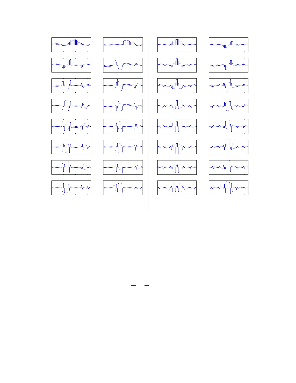
1 Optimizati on of Synthesis Ov ersampled Comple x Filter Banks J ´ er ˆ ome Gauthier , Student Member , IEEE , Laurent Duval, Member , IEEE and Jean-Christophe Pesquet, Senior Member , IEEE Abstract An impo rtant issue with oversampled FIR analysis filter bank s (FBs) is to determ ine inv erse synthesis FBs, when they exist. Gi ven any com plex oversampled FIR analysis FB, we first p rovide an algorithm to determin e whether there exists an in verse FIR synthesis system. W e also p rovide a method to ensure the Herm itian symmetry p roperty on the synth esis side, wh ich is serviceable to processing real-valued signals. As an inv ertible analysis scheme correspo nds to a red undan t decomp osition, ther e is no u nique in verse FB. Gi ven a p articular solutio n, we par ameterize the wh ole family of in verses through a nu ll space pro jection. The resulting r educed par ameter set simplifies d esign pr ocedures, since the perfect reconstruc tion constrain ed optimization pr oblem is recast as an u nconstrained op timization problem. The design of o ptimized synth esis FBs based on time o r fre quency localization criteria is then inv estigated, using a simple yet efficient gra dient a lgorithm. Index T erms Oversampled filter b anks, inversion, filter d esign, op timization, time localization, frequ ency localiza- tion, lapp ed tra nsforms, modu lated filter banks. I . I N T R O D U C T I O N Since the 70s, filter banks (FBs) h av e b ecome a ce ntral tool in sign al/image p rocessing and commu- nications: lapped or disc rete wa velet transforms can be viewed as instan ces of FB structures. Likewise, Copyrigh t (c) 2008 IEEE. Personal use of this material is permitted. Howe v er , permission to use this material for any other purposes must be obtained f rom the IEEE by sending a request t o pubs-permission s@ieee.org. L. Duv al is with the Institut Franc ¸ ais du P ´ etrole, IFP , T echno logy , Computer Science and Applied Mathematics Division, 1 et 4, aven ue de Bois-Pr ´ eau 92852 Rueil-Malmaison, France. E-mail: laurent.duv al@ifp.fr . J. Gauthier and J.-C . Pesquet are with the Institut Gaspard Monge and CNRS-UMR 804 9, Universit ´ e de Paris-Est, 77454 Marne-la-V all ´ ee Cedex 2, France. E-mail: { jerome.gauthier ,jean-christop he.pesquet } @un iv-p aris-est.fr . October 22, 2018 DRAFT 2 oversampled FBs (OFBs) c onstitute an exten si vely studied instance with remaining open que stions. Their development came along under a v ariety of dif ferent appellations, to name a few: gen eral A nalysis- Synthesis Systems [1 ], DF T (disc rete Fourier transform) with stack-shift capability , Overlap-Add or Generalized DFT , underdecimated systems , oversampled harmonic mod ulated filter b anks [2], [3], com- plex lapped transforms [4], ge neralized lapped ps eudo-biorthogon al transform, etc . In a more generic form, OF Bs hav e received a con siderable attention both theoretically and in many applications, in the past ten years, followi ng their association with specific types of frames [2], [5], [6]. Their design flexibility , improved frequen cy se lecti vity an d inc reased robustness to noise an d a liasing distortions hav e made them useful for subband a daptiv e filtering in audio processing [7], no ise s haping [8], den oising [3], multiple de scription coding [9], echo can cellation [10], multiple an tenna code de sign [11], ch annel equa lization [12 ], [13], [14] or channel coding [15]. T wo major problems arise wh en resorting to OFBs : ( i ) the existence of an in verse for the analys is OFB achieving perfect recon struction (PR) an d ( ii ) the d etermination of an “optimal” syn thesis FB . S ince the additional degrees of freedom gaine d through redund ancy may increase the d esign c omplexity , s ev eral works have focused on F Bs modulated with a single [16], [17] or multiple windo ws [18]. More ge neral formulations a re based on factorizations of OFB p olyphase rep resentations with additional cons traints (restricted oversampling ratios, symmetry , realness or filter length) into a lattice [19], [20], [21], [22 ] or a lifting structure [23]. Con structions with near pe rfect rec onstruction (relaxing the PR prope rty) have als o been propo sed [24 ], [25], [10], [26] . In [27], [28], [29], mo re in v olved alge braic tools (such a s Gr ¨ obne r bases ) have also been employed. Recen tly , Ch ai et al. have propo sed a des ign b ased o n FB state-sp ace representations [30]. The design ma y us e dif ferent kinds of optimization criteria b ased on filter regularity or more traditional cost functions base d on filter shape (su bband attenuation [21], [10], co ding gain [31]). Most of those synthe sis FB de signs re ly on minimum-norm solutions. An interesting a pproach c ombining the latters with a null sp ace method was s uccess fully pursued b y Mansou r [32] for s ynthesis window shape op timization in a modulated DFT FB. W i thin the c ompass of the prop osed work is a rela ti vely ge neric construction a nd optimization of oversampled sy nthesis filter ba nks with Finite Impu lse Resp onse (FIR) prope rties at b oth the analysis and s ynthesis sides. W e c an additionally impose a p ractically us eful He rmitian s ymmetry o n the s ynthesis side. This work exten ds the resu lts giv en in two previous conferen ce papers [33], [34]. A s pecial cas e has been judiciously devised in [22], for specific filter length a nd re dundancy factor allowing c losed form express ions for two d esign c riteria. In Sec tion II we rec all the polyph ase notation used throug hout this paper . Giv en a rbitrary FIR co mplex oversampled analysis FB, we first desc ribe in Se ction III-A October 22, 2018 DRAFT 3 a simple algorithm to test whe ther it is FIR in verti ble or not, b ased o n kn own res ults on polynomial matrices [35] , [36]. The standard Moore-Pe nrose ps eudo-in verse (PI) solution [37] is s tudied in Section III-B. In Sec tion III-C, a me thod is supplied to en force a n He rmitian sy mmetric FB, which is use ful for real d ata analysis, process ing and s ynthesis. In Section IV, the problem of the optimal design o f the synthesis FB is addresse d. A lthough optimization ca n be stud ied both on the analys is and synthe sis s ides [38], [39], we con sider here a giv en analysis FB and work on the synthe sis s ide. W e deriv e in Section IV -A an e f ficient parame ter set size reduction for this purpose . Using time or frequency loca lization criteria, we the n reformulate in Sec tion IV -B the constrained optimization problem a s a n unconstrained one for b oth the ge neral and He rmitian symme tric cas es. After desc ribing the optimization proces s, we illustrate, in S ection V, the different methods prop osed for the in version and optimization on three classical oversampled real a nd complex FB types. I I . P RO B L E M S TA T E M E N T A. Notations Processing . . . . . . . . . . . . . . . . . . . . . . . . . . . . . . . . . . . . . . . . . . . . . . . . . . . . . . . . . . . . . . . . . . . . . . . . . . . . . . . . . . . . . . . . . . . . . . . . . . . . . . . . . . . . . . . . . . . . . . . . . . . . . . . . . . . . . . . . . . . . . . . . . . . . . . . . . . . . . . . . . . . . . . . . . . . . . . . . . . . . . . . . . . . . . . . . . . . . . . . . . . . . . . . . . . . . . . . . . . . . . . . . . . . . . . . . . . . . . . . . . . . . . . . . . . . . . . . . . . . . . . . . . . . . . . . . . . . . . . . . . . . . . . . . . . . . . . . . . . . . . . . . . . . . . . . . . . . . . . . . . . . . . . . . . . . . . . . . . . . . . . . . . . . . . . . . . . . . . . . . . . . . . . . . . . . . . . . . . . . . . . . . . . . . . . . . . . . . . . . . . . . . . . . . . . . . . . . . . . . . . . . . . . . . . . . . . . . . . . . . . . . . . . . . . . . . . . . . . . . . . . . . . . . . . . . . . . . . . . . . . . . . . . . . . . . . . . . . . . . . . . . . . . . . . . . . . . . . . . . . . . . . . . . . . . . . . . . . . . . . . . . . . . . . . . . . . . ✲ ✲ ✲ ✲ ✲ ✲ ✲ ✲ ✲ ✲ y M − 1 ( n ) y 1 ( n ) y 0 ( n ) ↓ N ↓ N ↓ N H 0 H 1 H M − 1 . . . x n ↑ N ✲ ↑ N e H 0 e H 1 e H M − 1 . . . ↑ N ⊕ ✲ ✲ ✲ ✲ ✲ Fig. 1. Oversamp led M -channel filter bank. Lapped transforms [40] were introduced in [41] to avoid blocking artifacts in audio proces sing. Similarly for imag es, they reduce tiling ef fects produc ed by classica l block transforms (as can be seen in the JPEG image co mpression format). Lap ped trans forms b elong to the c lass of FBs, such as the one represented in Figure 1, with a de cimation factor N s maller than the length of eac h filter . The filters, whose impuls e response s are denote d by ( h i ) 0 ≤ i 1 . The M outputs of the analys is FB are d enoted by ( y i ( n )) 0 ≤ i N . T he following co nditions are equiv alent: 1) H [ z ] is “co prime”, which means that the determinants of the maximum minors (sub-matrices of size N × N ) are mu tually relatively prime. 2) H [ z ] is left in vertible in the se nse that there exists e H [ z ] ∈ C [ z , z − 1 ] N × M such tha t e H [ z ] H [ z ] = I N . A proo f of this result can be found in [35] for instanc e. The first cond ition is directly applicab le in prac tice to resolve the left in vertibility of the polyp hase transfer matrix. Using the follo wing procedure, we can ch eck numerically whethe r this co ndition is satisfied: ① Extract a maximal sub-matrix H e [ z ] of H [ z ] . ② Compute det( H e [ z ]) , and de termine its s et of roots S e . ③ Consider a nother ma ximal sub-matrix. Remove from S e the e lements which are not roots of the determinant of this sub -matrix. ④ Repeat step ③ until S e = ∅ or all max imal sub-matrices have been extracted. ⑤ If S e = ∅ then the polyph ase transfer matrix is left-in vertible; otherwise, it is not. The correspond ing a lgorithm is easily implemented, lea ding to extract the roots of a single polynomial and chec k the roots of a t most M N − 1 = M ! N !( M − N )! − 1 polyn omials. If the polyphas e matrix is left October 22, 2018 DRAFT 6 in vertible, the number of con sidered p olynomials in practice is u sually much s maller than M N − 1 , this bound being reac hed only when the ma trix is not in vertible. No te that in the c ase of caus al filters (i.e. both H [ z ] and e H [ z ] are polyn omial matrices in C [ z − 1 ] N × M ), simpler in vertibility con ditions exist by in voking the so-called c olumn-r educe d property [44], [45]. Also no tice that, one of the advantages of this algo rithm over other methods is that it can b e fully numerically implemented. B. Computation of an in verse FB The method propo sed in Section III-A only guarante es the existence of a left-in verse, c orresponding to an F IR synthe sis FB. Since it d oes not provide a c onstructiv e expres sion, we now perform the actual computation of a n in verse polyph ase transfer matrix. W e assume hereafter that H [ z ] was proven to be FIR left in vertible. Since the g oal is to achieve PR, we sea rch for a matrix e H [ z ] in C [ z , z − 1 ] N × M such that e H [ z ] H [ z ] = I N and there exists ( p 1 , p 2 ) ∈ N 2 such that the polyphase transfer function of the s ynthesis FB rea ds: e H [ z ] = P p 2 ℓ = − p 1 e H ( ℓ ) z − ℓ . The resulting overlapping factor of the s ynthesis filters is p = p 1 + p 2 + 1 . When working with Laurent p olynomial matrices , the se integers p 1 and p 2 are a pr iori unkn own, whereas with polynomial matrices a bound exists [44]. By rewriti ng the PR prop erty in block co n volutional form, we get the following linear s ystem: H e H = U (7) where U ⊤ = h 0 N ,p 1 N , I N , 0 N , ( p 2 + k − 1) N i ∈ R N × ( k + p − 1) N , e H ⊤ = h e H ( − p 1 ) , · · · , e H ( p 2 ) i ∈ C N × pM , (8) and H ⊤ = H (0) · · · H ( k − 1) 0 . . . . . . 0 H (0) · · · H ( k − 1) ∈ C pM × ( k + p − 1) N . (9) As already mentione d, p 1 and p 2 are unknown, but since the system (7) is sup posed in vertible, at least a cou ple of integers ( p 1 , p 2 ) solving the sy stem exists. The values of p 1 and p 2 are actua lly ob tained by inc reasing the value of p and loo king for every c ouple sa tisfying p = p 1 + p 2 + 1 , starting with p = 1 . Hence , for a g i ven p , we cons ider all ( p 1 , p 2 ) in { ( p − 1 , 0) , ( p − 2 , 1) , ..., (0 , p − 1 ) } . The first p allowing a Moore-Penros e pseudo-in verse [46] so lution to (7) provides an in verse p olyphase transfer matrix of minimum orde r . October 22, 2018 DRAFT 7 C. Hermitian sy mmetric case 1) Symmetry conditions: It is we ll known that the Fourier trans form of a real signal is Hermitian Symmetric (HS): its frequency decomposition is symme tric for the real pa rt a nd a nti-symmetric for the imaginary part. Con versely , if the co ef ficients are HS in the freque ncy doma in, then the recons tructed signal is rea l. This prope rty is very useful for real data filtering, which o ften consists of removing or thresholding co ef ficients in the frequ ency domain be fore recon structing. Securing the recon struction of real-valued signals from the transformed coe f ficients is thu s a d esirable prop erty . In this sec tion, we study the HS case and its effects on the methods prop osed in the previous s ections. The HS property in the synthes is filters is satisfied provided that, cons idering any symmetric subband indices j f ∈ { 0 , ..., M − 1 } and M − 1 − j f , for any coefficients ( y i ( n )) 0 ≤ i ǫ then increment n a nd go to step ② . The step-size µ n used here remains lar ge as long as the algorithm is getting c loser to a local minimum (in other words, as long as e J ( C n +1 ) < e J ( C n ) ). It is o nly adapted (redu ced) to prevent the criterion from increasing. The initialization with C 0 = 0 entails that we c onsider the pseud o-in verse synthes is FB as the starting po int for the algorithm. In practice, ǫ was set to 10 − 13 . Other step s election strategies exist: constan t or optimal steps, steps s atisfying W olfe or A rmijo conditions [49], [50]. T he metho d us ed in this work is easy to implement and is well-suited to the dif ferent co st functions we have co nsidered, while kee ping a rea sonable complexity . As the cos t func tions cons idered in this work are not conv ex, there is n o theoretical g uarantee that the algorithm co n verges to a global minimum. Y et, as is shown in Section V, initializing this metho d with the PI synthe sis FB provides quite good results and extens i ve simulations have confi rmed this good behaviour . The expres sion of the gradient for the gen eral c ost function is giv en in App endix A and is next applied to e J t and e J f in App endix B. D. Optimal so lution in the symmetric c ase 1) Cost functions: Using the same notations as in Sec tion IV -B, in the HS case, the follo wing form of the cost func tion is fou nd: J s ( e h ) = f J s ( C ) = M − 1 X j = 0 W j C + e H 0 j 2 K j W j C + e H 0 j 2 Λ . As in the gen eral case , (20) has b een us ed to trans form the c onstrained optimization problem on e h into an unc onstrained minimization problem on C . 2) Examples of cos t fun ctions: E quation (20) is very similar to (16). W e c onsequ ently de fine the cost functions in the HS case following the same approach as in Sections IV -B2 and IV -B3. Thus, the follo wing fun ctions are c onsidered: f J ts ( C ) = M − 1 X j = 0 W j C + e H 0 j 2 K t j W j C + e H 0 j 2 Λ , October 22, 2018 DRAFT 16 to co ncentrate the time localization o f impulse responses, and: f J fs ( C ) = M − 1 X j = 0 W j C + e H 0 j 2 K f j W j C + e H 0 j 2 Λ , to en hance the frequency selec ti v ity of the filters. Th eir gradients a re provided in Appendix C. V . E X A M P L E S As emphasized in the introduction, a wide variety of filter banks an d design c hoices can b e made. In this s ection, we ha ve c hosen to work with three dif ferent examples exhibiting interesting prop erties and allowi ng us to show the benefits incurred in the propo sed in version a nd optimization methods. A. Considered filter ba nks 1) Real Lapped T rans forms: T he study , developed for the ge neral complex c ase, remains fully a p- plicable to the design o f rea l filter b anks. As an illustration, we first conside r real lapp ed trans forms introduced in the middle o f the 90s under the na me of Gen LO T (ge neralized linear-phase lapped orthog- onal transform) [51]. Th ose transforms generalize the DCT (Discrete Cos ine T ran sform) and the LO T (lapped orthog onal transform). T o illustrate the in version method, we have ch osen a GenLO T with M = 16 filters of 32 coefficients. This FB is in vertible, in a no n standard oversampled use, with parameters N = 8 , k = 4 and k ′ = 2 . Its impulse and freque ncy res ponses a re repres ented in Figure 2. This F B is real and does n ot sa tisfy the HS condition. By u sing the method de scribed in Section III-B, we find p 1 = 3 and p 2 = 0 (hence p = 4 ). The freque ncy and impulse resp onses of the sy nthesis FB computed with the pseudo-in verse are shown on Figures 3(a) and 4(a). 2) Modulated c omplex lapp ed transform: W e now c onsider an other analysis FB bas ed on a wind owed generalized Fourier transform, c orresponding to a mo dulated co mplex lapped trans form ( MCLT ). This family of FB has b een used by Kingsbury [4] or Malvar [7] for applications in vide o as well as au dio process ing. The analysis impulse response s are: h i ( n ) = E ( i, n ) h a ( n ) , whe re E ( i, n ) = 1 √ k ′ N e − ı ( i − k ′ N 2 + 1 2 )( n − kN 2 + 1 2 ) 2 π k ′ N , and ( h a ( n )) 1 ≤ n ≤ k N is an analysis window . In this paper , we consider two analysis windo ws. The first, defined by ∀ n ∈ { 1 , ..., k N } , h a 1 ( n ) = sin nπ k N + 1 , October 22, 2018 DRAFT 17 0 10 20 30 −0.5 0 0.5 0 10 20 30 −0.5 0 0.5 0 10 20 30 −0.5 0 0.5 0 10 20 30 −0.5 0 0.5 0 10 20 30 −0.5 0 0.5 0 10 20 30 −0.5 0 0.5 0 10 20 30 −0.5 0 0.5 0 10 20 30 −0.5 0 0.5 0 10 20 30 −0.5 0 0.5 0 10 20 30 −0.5 0 0.5 0 10 20 30 −0.5 0 0.5 0 10 20 30 −0.5 0 0.5 0 10 20 30 −0.5 0 0.5 0 10 20 30 −0.5 0 0.5 0 10 20 30 −0.5 0 0.5 0 10 20 30 −0.5 0 0.5 0 0.1 0.2 0.3 0.4 0 2 4 0 0.1 0.2 0.3 0.4 0 2 4 0 0.1 0.2 0.3 0.4 0 2 4 0 0.1 0.2 0.3 0.4 0 2 4 0 0.1 0.2 0.3 0.4 0 2 4 0 0.1 0.2 0.3 0.4 0 2 4 0 0.1 0.2 0.3 0.4 0 2 4 0 0.1 0.2 0.3 0.4 0 2 4 0 0.1 0.2 0.3 0.4 0 2 4 0 0.1 0.2 0.3 0.4 0 2 4 0 0.1 0.2 0.3 0.4 0 2 4 0 0.1 0.2 0.3 0.4 0 2 4 0 0.1 0.2 0.3 0.4 0 2 4 0 0.1 0.2 0.3 0.4 0 2 4 0 0.1 0.2 0.3 0.4 0 2 4 0 0.1 0.2 0.3 0.4 0 2 4 (a) (b) Fig. 2. (a) Impulse and (b) frequenc y r esponses of a GenLO T analysis F B. is a standa rd sine window , e mployed for example in [7], [4]. The sec ond ( h a 2 ( n )) 1 ≤ n ≤ k N , c orresponds to a z ero-phase low-pass filter with cu tof f frequency 2 π / ( k N ) , built from a Kaiser window . This window , with be tter tapering than h a 1 , was used for instance in [32]. It is interesting to n ote that this a nalysis FB family , with both an alysis windows, satisfies Co ndition (11). In other words, it can be used to illustrate our ap proach in the HS case. The me thod from S ection III-A was employed to verify the in vertibility o n this FB, with both ana lysis wind ows and parameters N = 8 , k = 3 a nd k ′ = 7 / 4 . W e then comp ute a first synthes is FB with the PI me thod of Sec tion III-B. For the analysis FB with h a 1 window , the minimal parameters p 1 = 2 a nd p 2 = 0 we re obta ined. The frequen cy res ponse of this syn thesis FB is represented in Figure 5(a). In the h a 2 case, the minimal parameters p 1 = 2 a nd p 2 = 0 we re, on ce aga in, found when applying the method o f Section III-B. An HS synthesis FB is then d eri ved from this filter bank using October 22, 2018 DRAFT 18 0 0.1 0.2 0.3 0.4 0 2 4 0 0.1 0.2 0.3 0.4 0 1 2 0 0.1 0.2 0.3 0.4 0 1 2 0 0.1 0.2 0.3 0.4 0 2 4 0 0.1 0.2 0.3 0.4 0 1 2 0 0.1 0.2 0.3 0.4 0 1 2 0 0.1 0.2 0.3 0.4 0 1 2 0 0.1 0.2 0.3 0.4 0 2 4 0 0.1 0.2 0.3 0.4 0 1 2 0 0.1 0.2 0.3 0.4 0 1 2 0 0.1 0.2 0.3 0.4 0 1 2 0 0.1 0.2 0.3 0.4 0 1 2 0 0.1 0.2 0.3 0.4 0 1 2 0 0.1 0.2 0.3 0.4 0 1 2 0 0.1 0.2 0.3 0.4 0 2 4 0 0.1 0.2 0.3 0.4 0 2 4 0 0.1 0.2 0.3 0.4 0 2 4 0 0.1 0.2 0.3 0.4 0 1 2 0 0.1 0.2 0.3 0.4 0 1 2 0 0.1 0.2 0.3 0.4 0 1 2 0 0.1 0.2 0.3 0.4 0 1 2 0 0.1 0.2 0.3 0.4 0 1 2 0 0.1 0.2 0.3 0.4 0 1 2 0 0.1 0.2 0.3 0.4 0 1 2 0 0.1 0.2 0.3 0.4 0 1 2 0 0.1 0.2 0.3 0.4 0 1 2 0 0.1 0.2 0.3 0.4 0 1 2 0 0.1 0.2 0.3 0.4 0 1 2 0 0.1 0.2 0.3 0.4 0 1 2 0 0.1 0.2 0.3 0.4 0 1 2 0 0.1 0.2 0.3 0.4 0 1 2 0 0.1 0.2 0.3 0.4 0 2 4 (a) (b) Fig. 3. First example (wit h the GenLOT FB of Section V -A1): frequenc y response of the synthesis FB obtained (a) through the pseudo-in verse method and (b) after optimization w ith cost function e J t . the me thod o f Se ction III-C 2 to directly build an HS s ynthesis FB . The freque ncy and impulse respons es of the res ulting synthesis FBs, in the h a 2 case, are shown in Figures 6 a nd 7, respe cti vely . Figure 6(a) shows that synthesis filters p resent a sy mmetric behavior for their co ef ficients (in other words, they have a linea r p hase) while the synthesis FB in itself is not HS. W e also no tice that the frequency selectivity or time-frequency loca lization of the filters obtained through the ps eudo-in verse method s is n ot satisfactory . B. Optimization examples 1) K e rnel parameters: a) T empo ral kernel K t j : It is defin ed by (21). The parameters m j define the (tempo ral) pos itions around which the impulse respons es of the j th filter shou ld be con centrated. T o o btain well tapered October 22, 2018 DRAFT 19 0 10 20 30 −0.5 0 0.5 0 10 20 30 −0.5 0 0.5 0 10 20 30 −0.5 0 0.5 0 10 20 30 −0.5 0 0.5 0 10 20 30 −0.5 0 0.5 0 10 20 30 −0.5 0 0.5 0 10 20 30 −0.5 0 0.5 0 10 20 30 −0.5 0 0.5 0 10 20 30 −0.5 0 0.5 0 10 20 30 −0.5 0 0.5 0 10 20 30 −0.5 0 0.5 0 10 20 30 −0.5 0 0.5 0 10 20 30 −0.5 0 0.5 0 10 20 30 −0.5 0 0.5 0 10 20 30 −0.5 0 0.5 0 10 20 30 −0.5 0 0.5 0 10 20 30 −0.5 0 0.5 0 10 20 30 −0.5 0 0.5 0 10 20 30 −0.5 0 0.5 0 10 20 30 −0.5 0 0.5 0 10 20 30 −0.5 0 0.5 0 10 20 30 −0.5 0 0.5 0 10 20 30 −0.5 0 0.5 0 10 20 30 −0.5 0 0.5 0 10 20 30 −0.5 0 0.5 0 10 20 30 −0.5 0 0.5 0 10 20 30 −0.5 0 0.5 0 10 20 30 −0.5 0 0.5 0 10 20 30 −0.5 0 0.5 0 10 20 30 −0.5 0 0.5 0 10 20 30 −0.5 0 0.5 0 10 20 30 −0.5 0 0.5 (a) (b) Fig. 4. First example: impulse response of the synthesis FB obtained (a) through the pseudo -in verse method and (b) after optimization with cost function e J t . filters, we need to conc entrate the impu lse respon ses around the middle of the filter sup port. Therefore, the s ame pa rameter was used for all filters. The suppo rt o f the filters being {− p 1 N − N + 1 , ..., p 2 N } , we have chose n m j as ∀ 0 ≤ j < M , m j = m = p 2 N + 1 − p 1 N − N 2 . In ou r des ign exa mple, α ha s been set to 2 . b) F requency kern el K f j : It is defi ned by (23). The parameters f j represent the reduc ed frequenc ies around which we want to con centrate the frequ ency resp onses of the synthe sis filters. More precise ly , we chose f j such that it is centered inside the bandwidth of the analysis filter h j . The exponen t α has been se t to 2 . October 22, 2018 DRAFT 20 −0.5 0 0.5 0 5 10 −0.5 0 0.5 0 5 10 −0.5 0 0.5 0 5 10 −0.5 0 0.5 0 5 10 −0.5 0 0.5 0 5 10 −0.5 0 0.5 0 5 10 −0.5 0 0.5 0 5 10 −0.5 0 0.5 0 5 10 −0.5 0 0.5 0 5 10 −0.5 0 0.5 0 5 10 −0.5 0 0.5 0 5 10 −0.5 0 0.5 0 5 10 −0.5 0 0.5 0 5 10 −0.5 0 0.5 0 5 10 −0.5 0 0.5 0 1 2 3 −0.5 0 0.5 0 1 2 3 −0.5 0 0.5 0 1 2 3 −0.5 0 0.5 0 1 2 3 −0.5 0 0.5 0 1 2 3 −0.5 0 0.5 0 1 2 3 −0.5 0 0.5 0 1 2 3 −0.5 0 0.5 0 1 2 3 −0.5 0 0.5 0 1 2 3 −0.5 0 0.5 0 1 2 3 −0.5 0 0.5 0 1 2 3 −0.5 0 0.5 0 1 2 3 −0.5 0 0.5 0 1 2 3 −0.5 0 0.5 0 1 2 3 (a) (b) Fig. 5. Second example (in the MCL T case with window h a 1 ): frequenc y responses of synthesis fi lters (a) before and (b) aft er optimization with the cost function e J f . c) W eight parameters: In the propose d co st functions, the parameters ω t ,j and ω f ,j control the relati ve importance o f the different filters in the optimization p rocess. For the follo wing examples we have chosen equal we ights: ∀ j ∈ { 0 , ..., M − 1 } , ω t ,j = ω f ,j = 1 M . In othe r words, we aim at obtaining synthe sis filters with similar beh avior . 2) Computation time: I n Section IV -A, we have seen how to parameterize the system and thus how to reduce the dimens ion of the optimization problem. T o ev aluate the gain res ulting from this parameterization, Ma tlab programs were written to compa re the solutions of the cons trained problem, using function fmin con , w ith the so lutions of the unc onstrained p roblem, using fun ction fm inunc and using the gradient metho d explained in Sec tion IV -C. The two functions fmincon a nd fminunc were chos en as examp les of optimization implemen tation, while the grad ient proce dure can b e easily applied in d if ferent langu ages without requiring Matlab . The se programs were tested with the a nalysis October 22, 2018 DRAFT 21 0 5 10 15 20 25 0 5 10 0 5 10 15 20 25 0 0.5 1 0 5 10 15 20 25 0 5 10 0 5 10 15 20 25 0 5 10 15 0 5 10 15 20 25 0 2 4 6 0 5 10 15 20 25 0 2 4 6 0 5 10 15 20 25 0 5 10 15 0 5 10 15 20 25 0 5 10 0 5 10 15 20 25 0 0.5 1 0 5 10 15 20 25 0 5 10 0 5 10 15 20 25 0 5 10 15 0 5 10 15 20 25 0 2 4 6 0 5 10 15 20 25 0 2 4 6 0 5 10 15 20 25 0 5 10 15 0 5 10 15 20 25 0 2 4 6 0 5 10 15 20 25 0 5 10 0 5 10 15 20 25 0 5 10 0 5 10 15 20 25 0 2 4 6 0 5 10 15 20 25 0 5 10 0 5 10 15 20 25 0 5 10 0 5 10 15 20 25 0 2 4 6 0 5 10 15 20 25 0 2 4 6 0 5 10 15 20 25 0 5 10 0 5 10 15 20 25 0 5 10 0 5 10 15 20 25 0 2 4 6 0 5 10 15 20 25 0 5 10 0 5 10 15 20 25 0 5 10 0 5 10 15 20 25 0 2 4 6 (a) (b) Fig. 6. M odulus of the impulse responses of the synthesis FBs (in the MCL T case with h a 2 windo w): (a) pseudo-in verse and (b) symmetric version with the method of Section III-C2. FB introduced in Section V -A2 with the h a 1 window a nd the follo wing pa rameters: overlap factor k = 3 , redundan cy k ′ = 7 / 4 and downsampling N ∈ { 4 , 8 , 16 } . T he c ost func tion use d was J t (as d efined in Se ction IV -B2). T able I shows the computation time for the diff erent methods o n a co mputer with 2 . 16 GHz Intel Core 2 T 7400 CPU and 2 Gb of RA M. T ABLE I C O M P U T A T I O N T I M E T O O P T I M I Z E A S Y N T H E S I S F B W I T H D I FF E R E N T M E T H O D S U S I N G M A T L A B . N = 4 N = 8 N = 16 Constrained optimization (with fm incon ) 1 . 2 s 120 s 8800 s Unconstrained optimization (with fminunc ) 0 . 04 s 0 . 7 s 8 s Unconstrained optimization (gradient algorithm) 0 . 06 s 0 . 6 s 7 s A first interesting result is that all three me thods, starting from the sa me FB, con verge to almos t October 22, 2018 DRAFT 22 −0.5 0 0.5 0 20 40 60 −0.5 0 0.5 0 2 4 6 −0.5 0 0.5 0 20 40 60 −0.5 0 0.5 0 20 40 60 −0.5 0 0.5 0 10 20 30 −0.5 0 0.5 0 10 20 30 −0.5 0 0.5 0 20 40 60 −0.5 0 0.5 0 20 40 60 −0.5 0 0.5 0 2 4 6 −0.5 0 0.5 0 20 40 60 −0.5 0 0.5 0 20 40 60 −0.5 0 0.5 0 10 20 30 −0.5 0 0.5 0 10 20 30 −0.5 0 0.5 0 20 40 60 −0.5 0 0.5 0 10 20 30 −0.5 0 0.5 0 20 40 60 −0.5 0 0.5 0 20 40 −0.5 0 0.5 0 10 20 30 −0.5 0 0.5 0 20 40 −0.5 0 0.5 0 20 40 60 −0.5 0 0.5 0 10 20 30 −0.5 0 0.5 0 10 20 30 −0.5 0 0.5 0 20 40 60 −0.5 0 0.5 0 20 40 −0.5 0 0.5 0 10 20 30 −0.5 0 0.5 0 20 40 −0.5 0 0.5 0 20 40 60 −0.5 0 0.5 0 10 20 30 (a) (b) Fig. 7. Frequency responses of the synthesis FBs (in the MCL T case with h a 2 windo w): (a) pseudo-in verse and (b) symmetric version wit h the method of Secti on III- C2. identical synthe sis FBs. The c omputation times are howe ver very different: more than two h ours (with N = 16 ) for the cons trained o ptimization agains t a few s econds for the unco nstrained optimizations. W e can a lso n otice that the gradient algorithm is as fast as the fminunc Matlab function. This shows that the optimization me thod can b e easily implemented, through a gradien t algorithm, with no performance loss and without having to reso rt to the fminun c Matlab func tion 1 . In othe r words, this last result indicates that in some a pplicati ve contexts in wh ich Matlab is not avail able the optimization method ca n still be easily and ef ficiently implemented . 3) Examples of op timized FBs: In this se ction, we presen t optimization results 2 obtained with the dif ferent FBs introduced in Section V -A and us ing the different propos ed cost func tions. 1 This fairly sophisticated function uses an interior-reflectiv e Newton method [52]. 2 A matlab toolbox for FB optimization is av ailable here: http://www .laurent- duval.eu/misc- research- codes.html October 22, 2018 DRAFT 23 a) G eneral ca se: W e hav e a pplied the optimization method on the rea l FB introduce d in Sec- tion V -A1 with pa rameters: N = 8 , k = 4 and k ′ = 2 . The employed cost function is e J t . The result is shown in Figure 4 (b), the coe f fi cients before o ptimization (obtained with the pseudo-in verse method) are also displayed. It is clear that the impulse responses of op timized filters are b etter concentrated a round the middle of the su pport. Figu re 3 illustrates that the gain in time loca lization do es not e ntail a too severe loss in frequency selectivity of the o ptimized filters. A secon d o ptimization example is given using an MCL T F B with ana lysis window h a 1 and pa rameters N = 8 , k = 3 and k ′ = 7 / 4 . The resu lting frequency resp onses after optimization with cos t function e J f are represe nted in Figu re 5(b). W e observe that the frequency respo nses after optimization exhibit more regularity and an improved selec ti vity . The proposed cost functions take into acc ount a ll syn thesis filters at on ce. It therefore interesting to look mo re closely at each filter inde penden tly and determine whether the o ptimization leads to be tter results. In T able II, the frequ ency dispersion of each filter is reported before and after optimization with cost func tion e J f . In this case, the overall frequ ency dispersion o f the optimized filters has be en noticeably impro ved and sp read variabili ty ha s bee n drastically red uced. T ABLE II F R E Q U E N C Y D I S P E R S I O N O F T H E S Y N T H E S I S FI LT E R S O P T I M I Z E D W I T H C O S T F U N C T I O N e J f . Filter F req. disp. Filter F req. disp. e h 0 0 . 0290 e h opt 0 0 . 0111 e h 1 0 . 0851 e h opt 1 0 . 0110 e h 2 0 . 0569 e h opt 2 0 . 0109 e h 3 0 . 0606 e h opt 3 0 . 0112 e h 4 0 . 0658 e h opt 4 0 . 0110 e h 5 0 . 0596 e h opt 5 0 . 0109 e h 6 0 . 0363 e h opt 6 0 . 0111 e h 7 0 . 0156 e h opt 7 0 . 0111 e h 8 0 . 0411 e h opt 8 0 . 0109 e h 9 0 . 0231 e h opt 9 0 . 0110 e h 10 0 . 0508 e h opt 10 0 . 0112 e h 11 0 . 0499 e h opt 11 0 . 0110 e h 12 0 . 0574 e h opt 12 0 . 0109 e h 13 0 . 0521 e h opt 13 0 . 0111 Sum 0 . 6833 0 . 1544 October 22, 2018 DRAFT 24 b) R esults in the symmetric c ase: The optimization procedure was next applied in the HS c ase to the FB of Sec tion V -A2 (with ana lysis window h a 2 ). In this ca se, the cost functions f J ts and f J fs were employed. Once ag ain, the following parameters were used: N = 8 , k = 3 and k ′ = 7 / 4 . Figures 8 and 9 show the optimization results. W e ob serve that the o ptimizations with these two cos t func tions lead to FBs with different chara cteristics: a s expec ted, with f J ts the impulse respons es are better conc entrated than with f J fs and, conv e rsely , with f J fs the frequen cy se lecti vity is better than with f J ts . 0 5 10 15 20 25 0 2 4 6 0 5 10 15 20 25 0 5 10 0 5 10 15 20 25 0 5 10 0 5 10 15 20 25 0 2 4 6 0 5 10 15 20 25 0 5 10 0 5 10 15 20 25 0 5 10 0 5 10 15 20 25 0 2 4 6 0 5 10 15 20 25 0 2 4 6 0 5 10 15 20 25 0 5 10 0 5 10 15 20 25 0 5 10 0 5 10 15 20 25 0 2 4 6 0 5 10 15 20 25 0 5 10 0 5 10 15 20 25 0 5 10 0 5 10 15 20 25 0 2 4 6 0 5 10 15 20 25 0 1 2 0 5 10 15 20 25 0 1 2 0 5 10 15 20 25 0 1 2 0 5 10 15 20 25 0 1 2 0 5 10 15 20 25 0 1 2 0 5 10 15 20 25 0 1 2 0 5 10 15 20 25 0 1 2 0 5 10 15 20 25 0 1 2 0 5 10 15 20 25 0 1 2 0 5 10 15 20 25 0 1 2 0 5 10 15 20 25 0 1 2 0 5 10 15 20 25 0 1 2 0 5 10 15 20 25 0 1 2 0 5 10 15 20 25 0 1 2 0 5 10 15 20 25 0 2 4 6 0 5 10 15 20 25 0 2 4 6 0 5 10 15 20 25 0 2 4 6 0 5 10 15 20 25 0 2 4 6 0 5 10 15 20 25 0 2 4 6 0 5 10 15 20 25 0 2 4 6 0 5 10 15 20 25 0 2 4 6 0 5 10 15 20 25 0 2 4 6 0 5 10 15 20 25 0 2 4 6 0 5 10 15 20 25 0 2 4 6 0 5 10 15 20 25 0 2 4 6 0 5 10 15 20 25 0 2 4 6 0 5 10 15 20 25 0 2 4 6 0 5 10 15 20 25 0 2 4 6 (a) (b) (c) Fig. 8. Third example (in the MCL T case with window h a 2 ): modulus of the impulse responses of synthesis filters (a) before and after optimization (b) with the cost function f J ts and (c) with f J fs . 4) Compariso n: T o c onclude this example se ction, we propo se a compa rison with a n existing filter bank des ign. W e have chose n to compare our de sign methodology with the filter banks u sed in [7], [4]. In these works, the cons idered FBs corresp ond to a mod ulated complex lapped transform with overlap factor k = 2 an d redu ndancy k ′ = 2 . For this app lication, our choice of N = 8 results in the filters shown in [4]. The sy nthesis filter bank is then built w ith a metho d equiv alent to the weighted overlap-add technique. W e ha ve app lied the method s proposed in this work to c ompute an o ptimized synthe sis filter bank us ing the cost function f J ts . In T a ble III, the time dispersion of e ach syn thesis filter computed as October 22, 2018 DRAFT 25 −0.5 0 0.5 0 10 20 30 −0.5 0 0.5 0 20 40 60 −0.5 0 0.5 0 20 40 −0.5 0 0.5 0 10 20 30 −0.5 0 0.5 0 20 40 −0.5 0 0.5 0 20 40 60 −0.5 0 0.5 0 10 20 30 −0.5 0 0.5 0 10 20 30 −0.5 0 0.5 0 20 40 60 −0.5 0 0.5 0 20 40 −0.5 0 0.5 0 10 20 30 −0.5 0 0.5 0 20 40 −0.5 0 0.5 0 20 40 60 −0.5 0 0.5 0 10 20 30 −0.5 0 0.5 0 5 10 −0.5 0 0.5 0 2 4 6 −0.5 0 0.5 0 2 4 6 −0.5 0 0.5 0 2 4 6 −0.5 0 0.5 0 2 4 6 −0.5 0 0.5 0 2 4 6 −0.5 0 0.5 0 5 10 −0.5 0 0.5 0 5 10 −0.5 0 0.5 0 2 4 6 −0.5 0 0.5 0 2 4 6 −0.5 0 0.5 0 2 4 6 −0.5 0 0.5 0 2 4 6 −0.5 0 0.5 0 2 4 6 −0.5 0 0.5 0 5 10 −0.5 0 0.5 0 20 40 −0.5 0 0.5 0 20 40 −0.5 0 0.5 0 20 40 −0.5 0 0.5 0 20 40 −0.5 0 0.5 0 20 40 −0.5 0 0.5 0 20 40 −0.5 0 0.5 0 20 40 −0.5 0 0.5 0 20 40 −0.5 0 0.5 0 20 40 −0.5 0 0.5 0 20 40 −0.5 0 0.5 0 20 40 −0.5 0 0.5 0 20 40 −0.5 0 0.5 0 20 40 −0.5 0 0.5 0 20 40 (a) (b) (c) Fig. 9. Third ex ample (in the MCL T case with windo w h a 2 ): fr equenc y responses of synthesis filt ers (a) before and after optimization (b) with the cost function f J ts and (c) with f J fs . explained in [4] e h j j ∈{ 0 ,. .., 15 } and after optimization e h opt j j ∈{ 0 ,. .., 15 } are reported a s well a s the value of the cost func tion f J ts . Th e time d ispersion was clearly reduced with the propo sed method. V I . C O N C L U S I O N In this pap er , we have propos ed a me thod to tes t that a given oversampled FIR ana lysis FB is FIR in vertible and a method to compu te an op timized in verse FB. The optimization was performed for a clas s of cost functions allo wing either to emp hasize the time localization or the frequency selec ti vity of the filters. By rewriting the sy stem defining the synthe sis FB, we were able to parame terize the synthe sis filters for a g i ven filter length. This parameterization was then us ed to c on vert the constrained optimal synthesis prob lem into a n unco nstrained one, which can be solved with a s imple gradien t algorithm. The FB c onsidered here are o ne-dimensional; it would be interesting to study how the propo sed metho ds could be extended to the multidimension al ca se. Another perspective could be to study the cas e of FBs admitting an IIR left in verse that c an be approximated using a FIR FB with very long support. October 22, 2018 DRAFT 26 T ABLE III T I M E D I S P E R S I O N O F T H E S Y N T H E S I S FI LT E R S O P T I M I Z E D W I T H C O S T F U N C T I O N f J ts . Filter Time disp. Filter Time disp. e h 0 , e h 15 21 . 25 e h opt 0 , e h opt 15 2 . 4152 e h 1 , e h 14 21 . 25 e h opt 1 , e h opt 14 2 . 1064 e h 2 , e h 13 21 . 25 e h opt 2 , e h opt 13 2 . 3424 e h 3 , e h 12 21 . 25 e h opt 3 , e h opt 12 2 . 5516 e h 4 , e h 11 21 . 25 e h opt 4 , e h opt 11 2 . 5516 e h 5 , e h 10 21 . 25 e h opt 5 , e h opt 10 2 . 3424 e h 6 , e h 9 21 . 25 e h opt 6 , e h opt 9 2 . 1064 e h 7 , e h 8 21 . 25 e h opt 7 , e h opt 8 2 . 4152 f J ts 340 37 . 6626 A P P E N D I X A E X P R E S S I O N O F T H E G R A D I E N T In this first ap pendix, we study the g radient of e J (as defi ned in Section IV -B1) with respe ct to C . W e first ne ed to c alculate the gradient of f ( C ) = V j C + e H 0 j 2 K j . The matrix C b eing complex, we ha ve ∂ f ∂ C m,n = ∂ f ∂ C R m,n + ı ∂ f ∂ C I m,n = X i,i ′ ,ℓ,ℓ ′ ( V j ) i,m δ ℓ − n ( V j C + e H 0 j ) i ′ ,ℓ ′ + ( V j ) i ′ ,m δ ℓ ′ − n ( V j C + e H 0 j ) i,ℓ K j ( i, i ′ , ℓ, ℓ ′ ) + ı ı ( V j ) i,m δ ℓ − n ( V j C + e H 0 j ) i ′ ,ℓ ′ − ı ( V j ) i ′ ,m δ ℓ ′ − n ( V j C + e H 0 j ) i,ℓ K j ( i, i ′ , ℓ, ℓ ′ ) = 2 X i,i ′ ,ℓ ( V j ) i ′ ,m ( V j C + e H 0 j ) i,ℓ K j ( i, i ′ , ℓ, n ) . From this result, we deduce that ∇ e J ( C ) m,n = 2 M − 1 X j = 0 P i,i ′ ,ℓ ( V j ) i ′ ,m ( V j C + e H 0 j ) i,ℓ ( β j K j ( i, i ′ , ℓ, n ) − α j Λ( i, i ′ , ℓ, n )) β 2 j , (24) with α j = V j C + e H 0 j 2 K j and β j = V j C + e H 0 j 2 Λ . October 22, 2018 DRAFT 27 A P P E N D I X B E X A M P L E S O F G R A D I E N T S A first example is the calcu lation o f the gradient of the c ost function e J t . Applying (24) to the kernels ( K t j ) 0 ≤ j
Original Paper
Loading high-quality paper...
Comments & Academic Discussion
Loading comments...
Leave a Comment