Geodetic Line at Constant Altitude above the Ellipsoid

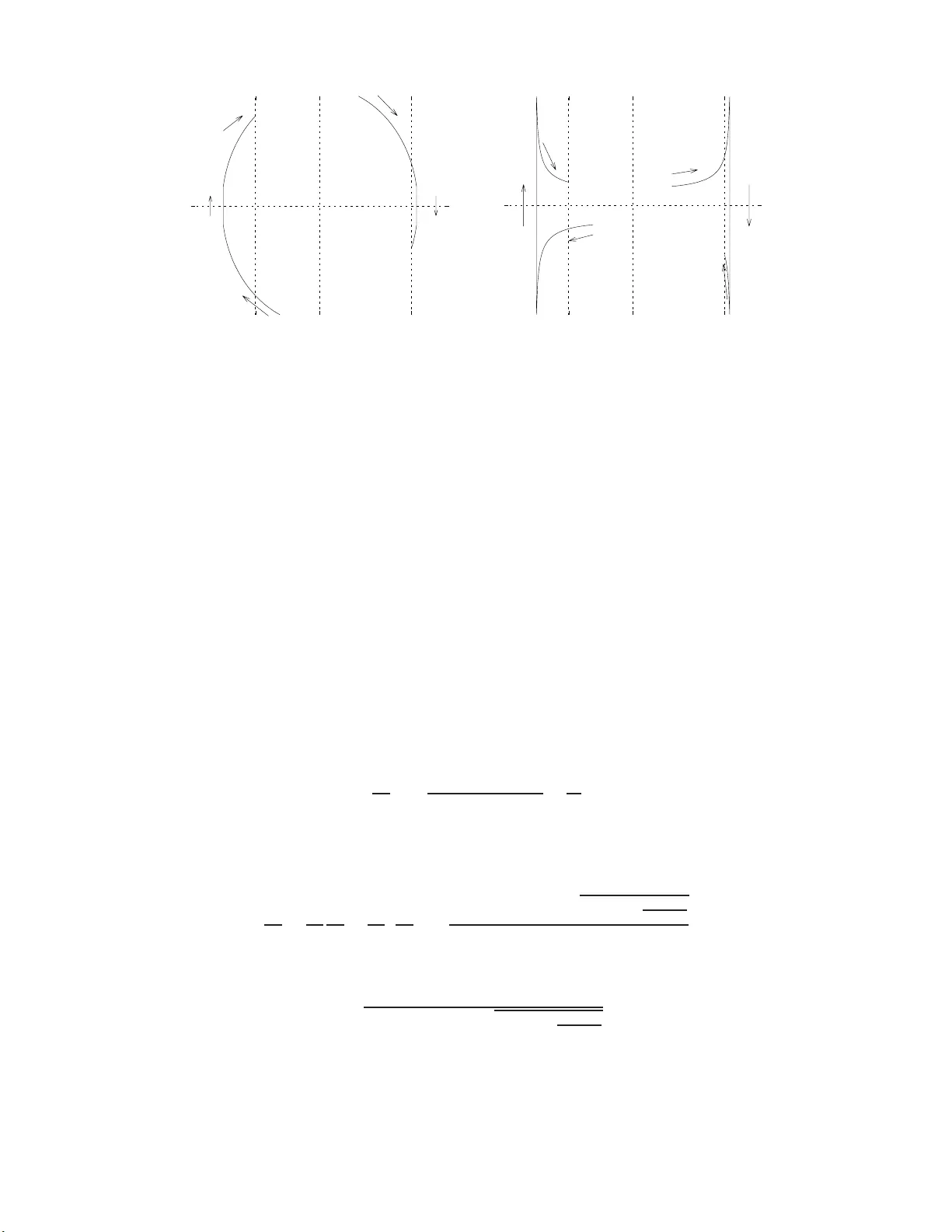
Geo detic Line at Constan t Altitude abov e the Ellipsoid Richard J. Matha r ∗ Max-Planck Institut f¨ ur Astr on omie, K¨ onigstuhl 17, 69117 Heidelb er g, Germany † (Dated: Decem b er 13, 202 2) The tw o-dimensional surface of a bi-axial ell ipsoid is c haracterized by the lengths of its ma jor and minor axes. Longitude and latitude span an angular co ordinate system across. W e consider the egg-shaped surface of constant a ltitude ab o ve (or b elo w) t he ellipsoid su rface, and compute the geodetic lines—lines of minim u m Euclidean length —within this surface whic h conn ect t w o p oints of fixed co ordinates. This addresses the common “inv erse” problem of geo d esics generalized to non-zero elev ations. The system of differential equations which couples the tw o angular co ordinates along the tra jectory is reduced to a single integral, which is h andled by T a ylor expan sion u p to fourth p ow er in the eccentricit y . P A CS num bers : 91.10.By , 91.10.Ws, 02.40.Hw Keyw ords: ge odesy; ell ipsoid; eccen tricity; geodetic line; inv erse problem I. CONTENTS The common three para meter s employed to relate Cartesia n coo rdinates to an ellipsoidal surface ar e the angles o f latitude and longitude in a grid on the surface, plus an altitude which is a shortest (p erp endicular) distance to the surface. The w ell-known functional r elations (co o r dinate transformations ) are summarized in Sec tion II . The inverse problem of geo desy is to find the line embedded in the ellipsoid surface which co nnects tw o fix e d p oints sub ject to minimization o f its length. W e p ose the equiv alent pro blem for lines at co nstant altitude, as if one would ask for the shor tes t track o f the center of a sphere of given r adius which ro lls on the ellipsoid s urface and meets t wo po in ts of the same, known altitude. In Sectio n II I , we fo r m ula te this in terms of the generic differential equations of geo desy parametrized by the Christoffel symbols. In the main Section IV , the coupled system of differential equatio ns of latitude and longitude as a function of pa th length is reduced to o ne degree of freedom, her e chosen to b e the directio n alo ng the path at one of the fix e d terminal po in ts , mea sured in the to po centric horizo n ta l system, and dubbed the launching angle. Closed-form ex pressions of this par ameter in terms of the co or dinates of the terminal po in ts hav e not b een fo und; instea d, the results are presented as s e r ies ex pa nsions up to fourth p ow er in the eccent ricity . The standard treatment of this analysis is the pro jection on an auxiliar y sphere; this technique is (almost) completely ignored but for the pragmatic a spec t that the cas e of zero eccentricit y is a suitable zeroth-or de r reference of series expansions around small ecce n tr ic ities. II. SPHER OIDAL COORDINA TES A. Surface The cros s sectio n o f an ellipsis of equator ial r adius ρ e > ρ p with eccentricit y e in a Cartesian ( x, z ) s ystem is: ρ 2 p = ρ 2 e (1 − e 2 ); x 2 ρ 2 e + z 2 ρ 2 p = 1 . (1) The ellipsis defines a geo centric latitude φ ′ and a geo detic latitude φ , the latter mea s ured by in tersection of the normal to the tangential pla ne with the equa to rial plane (Figure 1 ). On the surface of the e llipsoid [ 23 , § IX][ 5 ][ 2 , § 140 ]: tan φ = z x ρ 2 e ρ 2 p ; z x = tan φ ′ = ρ 2 p ρ 2 e tan φ. (2) ∗ mathar@mpia-hd.mpg.de ; https://www.mpia-hd.mpg.de/˜math ar † This w ork was supported b y the NW O VICI gran t 639.043.201 “Optical In terferometry: A new Method for Studies of Extrasolar Planets” to A. Quir ren bach. 2 φ φ x z ρ p ρ e v ’ ρ FIG. 1. Ma jor semi-axis ρ e , minor semi-axis ρ p , straight d istance to the center of co ordinates ρ , geo centric latitud e φ ′ , geod etic latitude φ , and their pointing difference v . Suppo sed ρ denotes the distance from the ce n ter of co ordinates to the point o n the geoid surface, the transformatio n from ( x, z ) to φ is x = ρ cos φ ′ = ρ e cos φ p 1 − e 2 sin 2 φ , z = ρ sin φ ′ = ρ e (1 − e 2 ) sin φ p 1 − e 2 sin 2 φ . (3) v = φ − φ ′ defines the difference b etw een the geo detic (astronomica l) and the geo cent ric latitudes, tan v = e 2 sin(2 φ ) 2(1 − e 2 sin 2 φ ) = m sin(2 φ ) 1 + m cos(2 φ ) = m s in(2 φ ) − m 2 sin(2 φ ) cos(2 φ ) + m 3 sin(2 φ ) cos 2 (2 φ ) + · · · ; (4) where the expansio n of the denominator has b een given in terms of the geo metric series of the para meter m ≡ e 2 2 − e 2 . (5) The T a ylo r series in p ow e rs o f sin(2 φ ) and in p ow ers of m ar e v = m 1 + m sin(2 φ ) + m 2 (2 + m ) 6(1 + m ) 3 sin 3 (2 φ ) + m 2 (5 + 2 5 m + 15 m 2 + 3 m 3 ) 40(1 + m ) 5 sin 5 (2 φ ) + · · · (6) = sin(2 φ ) m − 1 2 sin(4 φ ) m 2 + 1 3 sin(6 φ ) m 3 − 1 4 sin(8 φ ) m 4 + 1 5 sin(10 φ ) m 5 + · · · . (7) A flattening facto r f is also commo nly defined [ 10 ][ 19 , (3.14)], f = ρ e − ρ p ρ e = 1 − p 1 − e 2 ; e 2 = f (2 − f ) . (8) The reference v alues of the Earth ellipsoid adopted in the W GS84 [ 16 ] are f = 1 / 29 8 . 25722 3563 , ρ e = 6378 137 . 0 m . (9) B. General Altitude If one mov es along the direction of φ a distance h aw ay fr o m the sur face of the g eoid, the new co ordinates relative to ( 3 ) are [ 6 , 8 , 9 , 12 , 18 , 28 , 30 ] x = ρ cos φ ′ + h cos φ ; z = ρ sin φ ′ + h sin φ, (10) 3 h ρ (x 2 +y 2 ) (1/2) e φ N z FIG. 2. A p oint with Cartesian co ordinates ( x, y , z ) has a distance z to the eq uatorial plane, a d istance p x 2 + y 2 to the p olar axis, a distance h to the surface of the ellipsoid, and a distance N + h to the p olar axis, measured along t he local normal to the surface [ 13 ]. The vector e φ p oin ts North at this p oint. which ca n b e wr itten in terms of a distance N ( φ ), N ( φ ) ≡ ρ e p 1 − e 2 sin 2 φ (11) as x = ( N + h ) cos φ ; z = [ N (1 − e 2 ) + h ] sin φ. (12) Rotation of ( 12 ) around the p olar axis with g e ographic long itude λ defines the full 3D transfor mation be tw een ( x, y , z ) and ( λ, φ, h ),   x y z   =   [ N ( φ ) + h ] cos φ cos λ [ N ( φ ) + h ] cos φ sin λ  N ( φ )(1 − e 2 ) + h  sin φ   . (13) The only theme of this pap er is to generalize the geo detic lines of the literature [ 3 , 5 , 11 , 14 , 1 7 , 21 , 24 , 25 ] to the case of finite altitude h 6 = 0. The ph ys ics of gr avimetric or p otential theory is not inv o lv ed, only the mathematics of the geometr y . It sho uld be noted that p oints with constant, non-zero h do not define a surface of an ellips o id with effective semi-axes ρ e,p + h —otherwise the geo detic line c o uld b e deduced by mapping the problem onto an eq uiv alen t ellipsoidal surface [ 5 ]. II I. INVERSE PR OBLEM OF GEODESY A. T opo cen tric Co ordinate Sy s tem A line of shor test distance a t constant heig h t h = const b etw een tw o p oints 1 and 2 is defined b y minimizing the Euclidean distance, the line in teg ral S = Z 2 1 p dx 2 + dy 2 + dz 2 = Z 2 1 √ ds 2 ≡ Z 2 1 L ds (14) for some para metrization λ ( φ ). The integrand is equiv alent to a Lagra nge function L ( φ, λ, dλ/dφ ) or L ( φ, λ, dφ/dλ ). The gra dien t of ( 13 ) with resp ect to λ a nd φ defines the vectors e λ,φ that span the top o centric tang en t plane e λ =   − [ N ( φ ) + h ] cos φ sin λ [ N ( φ ) + h ] cos φ cos λ 0   ; e φ =   − sin φ co s λ [ M ( φ ) + h ] − sin φ sin λ [ M ( φ ) + h ] cos φ [ M ( φ ) + h ]   , (15) 4 where a meridional r adius of curv ature [ 26 ][ 19 , (3.87)] M ( φ ) ≡ ρ e (1 − e 2 ) (1 − e 2 sin 2 φ ) 3 / 2 = N ( φ ) 1 − e 2 1 − e 2 sin 2 φ (16) is defined to simplify the notation. Building squares and dot pro ducts computes the three Ga us s F undamental parameters of the surfa c e [ 20 ] e 2 λ = E = ( N + h ) 2 cos 2 φ ; (17) e λ · e φ = F = 0; (18) e 2 φ = G =  N 1 − e 2 1 − e 2 sin 2 φ + h  2 = ( M + h ) 2 . (19) Spec ia lizing to h = 0 we ge t the Y o u formulae [ 29 ]. E a nd G provide the principal curv atures along the meridian and azimuth [ 4 ], and the co efficients of the metric tensor in the q uadratic form of ds 2 , S = Z p E dλ 2 + 2 F dλdφ + Gdφ 2 . (20) B. Christoffel Symbols Christoffel symbols are the co nnection co efficients b et w een differ e n tials d e ǫ of the top o centric axis a nd of the po sitions d x β , in a generic definition d e ǫ = X α,β e α Γ α β ǫ d x β . (21) This format is matched b y first computing the der iv ative o f e λ with resp ect to λ and φ (at h = const ): d e λ =   − ( N + h ) cos φ cos λ − ( N + h ) cos φ sin λ 0   dλ +   ( M + h ) sin φ sin λ − ( M + h ) sin φ cos λ 0   dφ (22) and of e φ with re s pect to λ and φ : d e φ =   ( M + h ) sin φ sin λ − ( M + h ) sin φ cos λ 0   dλ +      h N e 2 cos 2 φ 1 − e 2 sin 2 φ − 3 N e 2 (1 − e 2 ) sin 2 φ (1 − e 2 sin 2 φ ) 2 − ( N + h ) i cos φ cos λ h N e 2 cos 2 φ 1 − e 2 sin 2 φ − 3 N e 2 (1 − e 2 ) sin 2 φ (1 − e 2 sin 2 φ ) 2 − ( N + h ) i cos φ sin λ h N e 2 (1 − e 2 )  3 cos 2 φ (1 − e 2 sin 2 φ ) 2 − sin 2 φ 1 − e 2 sin 2 φ  − [ N (1 − e 2 ) + h ] i sin φ      dφ. (23) The next step splits these tw o equations to the expanded version of ( 21 ), d e λ = ( e λ Γ λ λλ + e φ Γ φ λλ ) dλ + ( e λ Γ λ φλ + e φ Γ φ φλ ) dφ ; (24) d e φ = ( e λ Γ λ λφ + e φ Γ φ λφ ) dλ + ( e λ Γ λ φφ + e φ Γ φ φφ ) dφ. ( 25) The eight Γ ar e extracted by ev aluating do t pro ducts of the four vector coe fficie n ts in ( 22 )–( 23 ) by e λ and e φ , Γ λ λλ = Γ φ φλ = Γ φ λφ = Γ λ φφ = 0; (26) Γ φ λλ = ( N + h ) cos φ sin φ 1 − e 2 sin 2 φ h (1 − e 2 sin 2 φ ) + N (1 − e 2 ) ; (27) Γ λ φλ = Γ λ λφ = − sin φ h (1 − e 2 sin 2 φ ) + N (1 − e 2 ) ( N + h )(1 − e 2 sin 2 φ ) cos φ ; (28) 5 Γ φ φφ = 3 N e 2 (1 − e 2 ) sin φ cos φ 1 [ h (1 − e 2 sin 2 φ ) + N (1 − e 2 )](1 − e 2 sin 2 φ ) . (29) The E uler-Lagr ange Differential Equations δ R 2 1 p E dλ 2 + Gdφ 2 = 0 for a stationa ry Lagra nge dens it y L (at F = 0 ) bec ome the differential equations of the geo desic [ 20 ], in the generic for mat d 2 x ǫ ds 2 + X µν Γ ǫ µν dx µ ds dx ν ds = 0 . (30) The explicit wr ite-up d 2 λ ds 2 + Γ λ λλ dλ ds dλ ds + Γ λ λφ dλ ds dφ ds + Γ λ φλ dφ ds dλ ds + Γ λ φφ dφ ds dφ ds = 0; (31) d 2 φ ds 2 + Γ φ λλ dλ ds dλ ds + Γ φ λφ dλ ds dφ ds + Γ φ φλ dφ ds dλ ds + Γ φ φφ dφ ds dφ ds = 0 , (32) simplifies with ( 26 ) to d 2 λ ds 2 + 2Γ λ λφ dλ ds dφ ds = 0; (33) d 2 φ ds 2 + Γ φ λλ  dλ ds  2 + Γ φ φφ  dφ ds  2 = 0 . (34) IV. REDUCTION OF THE DIF FERENTIAL EQUA TIONS A. Separation of Angular V ariables Decoupling of the tw o different ial equations ( 33 )–( 34 ) starts with the separation of v aria bles in ( 33 ), d 2 λ ds 2 dλ ds = − 2 Γ λ φλ dφ ds . (35) Change of the integration v ariable on the right hand side from s to φ allows to use the underiv ative of ( 28 ) Z Γ λ λφ ( φ ) dφ = log { [ N ( φ ) + h ] cos φ } + const (36) to generate a firs t integral log dλ ds = − 2 lo g[( N + h ) cos φ ] + const. (37) Exp onentiation yields dλ ds = c 3 1 ( N + h ) 2 cos 2 φ , (38) where c 3 ≡ dλ ds | 1 ( N 1 + h ) 2 cos 2 φ 1 (39) is a constant for each geo desic; it plays the role of the Clairaut cons tan t [ 22 , 27 ], but has length units in our ca se. It has b een defined with the azimuth φ 1 and N 1 ≡ N ( φ 1 ) at the start of the line, but could as well b e a sso ciated with any other p oin t or the end p oint 2. c 3 is p ositive for tra jector ies sta r ting into ea st w ards direction, negative for the west wards hea ding, zero for routes to the p oles. Moving the squar e of ( 38 ) into ( 34 ) yields d 2 φ ds 2 + sin φ ( N + h ) 3 cos 3 φ 1 − e 2 sin 2 φ h (1 − e 2 sin 2 φ ) + N (1 − e 2 ) c 2 3 + 3 N e 2 (1 − e 2 ) sin φ cos φ [ h (1 − e 2 sin 2 φ ) + N (1 − e 2 )](1 − e 2 sin 2 φ )  dφ ds  2 = 0 . ( 40) 6 T o so lv e this differential equa tion, w e substitute the v aria ble φ by its pro jection τ on to the po lar axis, τ ≡ sin φ, (41) which implies tra nsformations in the deriv atives: dτ ds = cos φ dφ ds ; (42) d 2 τ ds 2 = − sin φ dφ ds dφ ds + cos φ d 2 φ ds 2 ; (43) cos φ d 2 φ ds 2 = d 2 τ ds 2 + τ  dφ ds  2 = d 2 τ ds 2 + τ cos 2 φ  dτ ds  2 = d 2 τ ds 2 + τ 1 − τ 2  dτ ds  2 . (44) W e multiply ( 40 ) by cos φ , then replace dφ/ds and d 2 φ/ds 2 as noted ab ov e, d 2 τ ds 2 + τ 1 − τ 2  dτ ds  2 + τ ( N + h ) 3 (1 − τ 2 ) 1 − e 2 τ 2 h (1 − e 2 τ 2 ) + N (1 − e 2 ) c 2 3 + 3 N e 2 (1 − e 2 ) τ [ h (1 − e 2 τ 2 ) + N (1 − e 2 )](1 − e 2 τ 2 )  dτ ds  2 = 0; d 2 τ ds 2 + τ 1 − τ 2 h (1 − e 2 τ 2 ) 2 + N (1 − 4 e 2 τ 2 + 2 e 2 + 4 e 4 τ 2 − 3 e 4 ) [ h (1 − e 2 τ 2 ) + N (1 − e 2 )][1 − e 2 τ 2 ]  dτ ds  2 + τ ( N + h ) 3 (1 − τ 2 ) 1 − e 2 τ 2 h (1 − e 2 τ 2 ) + N (1 − e 2 ) c 2 3 = 0 . (45) This is a differential equation with no explicit appe a rance of the indep endent v ar iable s , (1 − τ 2 ) d 2 τ ds 2 + h (1 − e 2 τ 2 ) 2 + N (1 − e 2 )(1 + 3 e 2 − 4 e 2 τ 2 ) [ h (1 − e 2 τ 2 ) + N (1 − e 2 )][1 − e 2 τ 2 ] τ  dτ ds  2 + τ c 2 3 ( N + h ) 3 1 − e 2 τ 2 h (1 − e 2 τ 2 ) + N (1 − e 2 ) = 0 , and the standard way of prog ressing is the substitution dτ ds ≡ p ; d 2 τ ds 2 = p dp dτ ; (46) (1 − τ 2 ) p dp dτ + h (1 − e 2 τ 2 ) 2 + N (1 − e 2 )(1 + 3 e 2 − 4 e 2 τ 2 ) [ h (1 − e 2 τ 2 ) + N (1 − e 2 )][1 − e 2 τ 2 ] τ p 2 + τ c 2 3 ( N + h ) 3 1 − e 2 τ 2 h (1 − e 2 τ 2 ) + N (1 − e 2 ) = 0 . (47) This is transfo r med to a linear differential equa tio n by the further substitution P ≡ p 2 , dP / dτ = 2 p dp/dτ , 1 2 (1 − τ 2 ) dP dτ + h (1 − e 2 τ 2 ) 2 + N (1 − e 2 )(1 + 3 e 2 − 4 e 2 τ 2 ) [ h (1 − e 2 τ 2 ) + N (1 − e 2 )][1 − e 2 τ 2 ] τ P + τ c 2 3 ( N + h ) 3 1 − e 2 τ 2 h (1 − e 2 τ 2 ) + N (1 − e 2 ) = 0 . (48) The standar d appro ach is to solve the homog eneous differen tia l e q uation first, dP dτ = − 2 τ h (1 − e 2 τ 2 ) 2 + N (1 − e 2 )(1 + 3 e 2 − 4 e 2 τ 2 ) [1 − τ 2 ][ h (1 − e 2 τ 2 ) + N (1 − e 2 )][1 − e 2 τ 2 ] P. (49) After divisio n throug h P , the left hand s ide is easily in teg rated, and the r ight hand side (incompletely) deco mpos e d int o partial fractions , log P = − 2 Z τ h (1 − e 2 τ 2 ) 2 + N (1 − e 2 )(1 + 3 e 2 − 4 e 2 τ 2 ) [1 − τ 2 ][ h (1 − e 2 τ 2 ) + N (1 − e 2 )][1 − e 2 τ 2 ] dτ = Z − 2 τ 1 − τ 2 dτ + 3 Z − 2 e 2 τ 1 − e 2 τ 2 dτ + 6 he 2 Z τ h (1 − e 2 τ 2 ) + N (1 − e 2 ) dτ = log (1 − τ 2 ) + 3 log(1 − e 2 τ 2 ) − 2 log h h (1 − e 2 τ 2 ) 3 / 2 + ρ e (1 − e 2 ) i + const. (50) 7 P = const · (1 − τ 2 )(1 − e 2 τ 2 ) 3  h (1 − e 2 τ 2 ) 3 / 2 + ρ e (1 − e 2 )  2 = const · (1 − τ 2 )(1 − e 2 τ 2 ) 2 [ h (1 − e 2 τ 2 ) + N (1 − e 2 )] 2 = const · (1 − τ 2 ) G ( τ ) . Solution of the inhomo gene ous differen tia l e q uation ( 48 ) pro ceeds with the v a r iation o f the constant, the ansatz P = c ( τ ) · (1 − τ 2 )(1 − e 2 τ 2 ) 2 [ h (1 − e 2 τ 2 ) + N (1 − e 2 )] 2 . (51) Back insertion into ( 48 ) leads to a first order different ial equatio n for c ( τ ), dc ( τ ) dτ 1 − τ 2 G ( τ ) = − 2 τ c 2 3 (1 − τ 2 )( N + h ) 3 1 − e 2 τ 2 h (1 − e 2 τ 2 ) + N (1 − e 2 ) , which is deco mpose d into partial fractions dc ( τ ) dτ = c 2 3  eN 2 eτ 1 − e 2 τ 2 1 ( N + h ) 3 + − 2 τ 1 − τ 2 1 ( N + h ) 2  1 1 − τ 2 . The ensuing integral over dτ is solved by aid of the substitution τ 2 = u , c ( τ ) = − c 2 3 1 ( N + h ) 2 (1 − τ 2 ) + const. Back into ( 51 )—using const to indica te placemen t of any member of an anonymous bag of constants of integration, P =  const − 1 ( N + h ) 2 (1 − τ 2 )  c 2 3 (1 − τ 2 )(1 − e 2 τ 2 ) 2 [ h (1 − e 2 τ 2 ) + N (1 − e 2 )] 2 (52) = c 5 (1 − τ 2 )(1 − e 2 τ 2 ) 2 [ h (1 − e 2 τ 2 ) + N (1 − e 2 )] 2 − c 2 3 (1 − e 2 τ 2 ) 2 ( N + h ) 2 [ h (1 − e 2 τ 2 ) + N (1 − e 2 )] 2 (53) = c 5 1 ( h + M ) 2  1 − τ 2 − c 2 3 ( N + h ) 2  = c 5 1 − τ 2 G ( τ )  1 − c 2 3 E ( τ )  = p 2 . (54) The subscript 1 denotes v alue s at the starting p oint of the curve, P 1 = c 5 cos 2 φ 1 (1 − e 2 sin 2 φ 1 ) 2  h (1 − e 2 sin 2 φ 1 ) + N 1 (1 − e 2 )  2 − c 2 3 (1 − e 2 sin 2 φ 1 ) 2 ( N 1 + h ) 2  h (1 − e 2 sin 2 φ 1 ) + N 1 (1 − e 2 )  2 = p 2 1 (55) = c 5 cos 2 φ 1 (1 − e 2 sin 2 φ 1 ) 2  h (1 − e 2 sin 2 φ 1 ) + N 1 (1 − e 2 )  2 − ( dλ/ds ) 2 1 ( N 1 + h ) 2 cos 4 φ 1 (1 − e 2 sin 2 φ 1 ) 2  h (1 − e 2 sin 2 φ 1 ) + N 1 (1 − e 2 )  2 . (56) Solving for c 5 yields c 5 =  dλ ds | 1  2 cos 2 φ 1 ( N 1 + h ) 2 + p 2 1  h (1 − e 2 sin 2 φ 1 ) + N 1 (1 − e 2 )  2 cos 2 φ 1 (1 − e 2 sin 2 φ 1 ) 2 =  dλ ds | 1  2 cos 2 φ 1 ( N 1 + h ) 2 + p 2 1 cos 2 φ 1 G 1 =  dλ ds | 1  2 E 1 +  dφ ds | 1  2 G 1 = c 2 3 ( N 1 + h ) 2 cos 2 φ 1 +  dφ ds | 1  2 ( M 1 + h ) 2 . (57) Compared with the differ en tia l version of ( 20 ), ds 2 = E dλ 2 + Gdφ 2 ; 1 = E  dλ ds  2 + G  dφ ds  2 , (58) we m ust hav e c 5 = 1. Note that ( 54 ) is essentially a write-up for p 2 ∼ ( dφ/ds ) 2 and co uld b e derived quickly b y inserting ( 38 ) directly in to ( 58 ). The squar e ro ot of ( 54 ) is p = ± 1 − e 2 τ 2 h (1 − e 2 τ 2 ) + N (1 − e 2 ) s 1 − τ 2 − c 2 3 ( N + h ) 2 = ± q 1 − τ 2 − c 2 3 ( N + h ) 2 h + M ( τ ) = dτ ds . (59) 8 τ d τ /ds τ 2 τ 2 τ 1 τ m τ m τ 1 τ 2 τ 2 τ ds/d τ τ 2 τ 2 τ 1 τ m τ m τ 1 τ 2 τ 2 FIG. 3. Tw o examples of tra jectories of dτ /ds [left, equation ( 59 )] or ds/dτ [right] as a function of τ . They may or may not p ass through a zero τ m of ( 59 ) while connecting the starting abscissa τ 1 with the fi nal abscissa τ 2 . There are four basic top ologi es, dep ending on whether τ m is p ositive or negative, and dep ending on whether the sign c h ange in dτ /ds is from + t o − or from − to + at this p oint. The sign in front o f the s quare ro ot is to b e chosen p ositive for pieces of the tra jectory with dτ /ds > 0 (northern direction), negative wher e dτ /ds < 0 (souther n direction). The v alue in the s quare ro ot may run through zero within one curve, dτ /ds = 0 at one p oint τ m , such that the square ro ot switches sign there (Figure 3 ). This happens whenever (1 − τ 2 m )[ N ( τ m ) + h ] 2 = c 2 3 (60) yields a v anishing discr iminan t of the square ro ot for some ( λ, φ ), that is, whenever the difference λ 2 − λ 1 is sufficiently large to cre a te a point of minim um p olar distance along the tra jectory that is not one o f the terminal po in ts. B. Launching Direction So far we hav e written the bundle of all geo desics through ( λ 1 , φ 1 ) in the forma t ( 59 ), which spec ifie s the change of latitude as a function of distance traveled. The dir ection at p oint 1 in the top o centric system of co ordinates is represented by c 3 . T o address the in verse problem of geo desy , that is to pic k the particula r geo desics whic h als o runs through the terminal po in t ( λ 2 , φ 2 ) in fulfillmen t of the Dirichlet b oundary conditions, the asso ciated change in longitude, some form o f ( 38 ), dλ ds = c 3 1 ( N + h ) 2 (1 − τ 2 ) = c 3 E , (61) m ust obviously get in volv ed. The stra tegy is to write down τ ( λ ) o r λ ( τ ) with c 3 as a par ameter, then to adjust c 3 to ensure with what would be ca lled a s hoo ting metho d that s ta rting at po int 1 at that a ngle eventu ally pass es through po in t 2. Coupling o f λ to τ is done by divisio n o f ( 59 ) and ( 61 ), dτ dλ = dτ ds ds dλ = dτ ds / dλ ds = ± ( N + h ) 2 (1 − τ 2 ) q 1 − τ 2 − c 2 3 ( N + h ) 2 c 3 ( h + M ) . (62) Separation of b oth v aria bles yields ± Z 1 dτ c 3 ( h + M ) ( N + h ) 2 (1 − τ 2 ) q 1 − τ 2 − c 2 3 ( N + h ) 2 = λ | 1 . (63) An approa c h of ev aluating the integral by p ow er series e x pansion in h/ρ e is prop osed in [ 15 ]. F or sho r t paths, s mall | λ 2 − λ 1 | , the integral is simply R τ 2 τ 1 . If one of the cases o c curs, where the difference in λ is to o la rge for a solution, the additional path through the sing ula rity τ m is to b e use d [with s o me lo cal ex trem um in the g raph τ ( s )], and the integral is to b e interpreted as R τ m τ 1 − R τ 2 τ m . T aking the sig n change and the symmetry 9 of the integrand into a c coun t, this is R τ 2 τ 1 +2 R τ m τ 2 = R τ m τ 1 + R τ m τ 2 , twice the underiv ative at τ m min us the s um of the underiv ative a t τ 1 and τ 2 . In the r ight plot o f Figure 3 , the difference is in including or not including the lo udspea k er shap ed area b et ween τ 2 and τ m . τ m is the solution of ( 60 ), the p ositive v alue of the solution taken if dτ /ds > 0 at φ 1 , the negative v a lue if dτ / ds < 0 at φ 1 . T he squared zero of dτ /ds , τ 2 m , is a ro ot of the fourth-order poly nomial which emer g es by rewriting ( 60 ), e 4 h 4 ( τ 2 m ) 4 + 2 e 2 h 2  ρ 2 e − h 2 + e 2  c 2 3 − h 2  ( τ 2 m ) 3 + h  ρ 2 e − h 2  2 + 2 e 2  2 h 4 − 2 c 2 3 h 2 − 2 ρ 2 e h 2 − ρ 2 e c 2 3  + e 4  c 2 3 − h 2  2 i ( τ 2 m ) 2 + 2 h −  ρ 2 e − h 2  2 + c 2 3  ρ 2 e + h 2  + e 2  −  c 2 3 − h 2  2 + ρ 2 e ( c 2 3 + h 2 ) i τ 2 m +  ( ρ e + h ) 2 − c 2 3   ( ρ e − h ) 2 − c 2 3  = 0 . (64) Alternatively , τ m admits a T a ylo r ex pa nsion by expanding the ze ro o f ( 60 ) in orde r s o f e : ± τ m = r 1 − c 2 3 H 2 + c 2 3 ρ e 2 H 3 r 1 − c 2 3 H 2 e 2 − 3 c 2 3 ρ e 8 H 3 "  ρ e H − c 2 3 H 2  2 − 1 # r 1 − c 2 3 H 2 e 4 + O ( e 6 ) , (65) where some maximum distance H ≡ ρ e + h (66) to the p olar axis has b een defined to condense the notation. The integrand in ( 63 ) has a T aylor expansion in e , ± Z dτ    c 3 / ( ρ e + h ) (1 − τ 2 ) q 1 − τ 2 − c 2 3 ( ρ e + h ) 2 − c 3 ρ e [( ρ e + h ) 2 (2 − τ 2 ) − 2 c 2 3 ] 2( ρ e + h ) 4  1 − τ 2 − c 2 3 ( ρ e + h ) 2  3 / 2 e 2 + O ( e 4 )    = λ | 1 . (67) W e integrate the left hand side of ( 67 ) sepa rately for each p ow er of e up to O ( e 4 ), h arctan τ c 3 H √ T − c 3 ρ e 2 H 2  τ √ T + arctan τ √ T  e 2 − c 3 ρ e 16 H 7  τ T 3 / 2 [ − 2 H 2 c 2 3 ρ e + 4 H 2 c 2 3 ρ e T + 2 c 4 3 ρ e − 6 H 3 c 2 3 T + 6 H 5 T − 9 H 5 T 2 − 4 H 4 ρ e T + 6 H 4 ρ e T 2 ] + H 2 [3 H 3 − 2 ρ e H 2 − 3 c 2 3 H + 4 c 2 3 ρ e ] arctan τ √ T  e 4 + O ( e 6 ) i τ 2 τ 1 = ± ( λ 2 − λ 1 ) , (68) where T ≡ 1 − τ 2 −  c 3 H  2 (69) is some conv enient definition of the tra jector y ’s distance to its solstice τ m . The fir st term is no t the principa l v alue of the arc tang e n t but its steadily defined ex tens ion thro ugh the entire interv al of τ -v alues, | τ | ≤ τ m . It is an o dd function of τ , and phase jumps ar e corrected as follows: the inclination at τ = 0 has (by insp e ction of the deriv ative ab ov e a t τ = 0) the sig n of c 3 . So whenever the triple pro duct sgn τ sg n c 3 sgn(arctan . ) is neg a tiv e, o ne must shift the branch of the a rctan by adding multiples of π sg n τ sgn c 3 to the principal v alue. Whether this is to b e taken b etw een the limits τ 2 and τ 1 or as the s um of tw o comp onents (see ab ov e) can b e tested b y integrating up to τ m , R τ m τ 1 , where the v alue of the underiv ative at τ m is g iv en by (1 / 2) arctan 0, e ffectiv ely π 2 sgn τ m sgn c 3 after selecting the branch of the inv erse trigonometric function as descr ibed ab ov e. Equation ( 68 ) is solved numerically , wher e c 3 /H is the unknown, where τ 1 , 2 and λ 1 , 2 are known fr o m the co or - dinates of the tw o po in ts that define the boundar y v alue problem, and wher e e and H are constant par ameters. The complexity of the equation sugg ests use of a Newton algor ithm to search fo r the zero , star ting fro m ( A19 ), c 3 /H ≈ cos φ 1 cos φ 2 sin( λ 2 − λ 1 ) / sin Z , a s the initial estimate. An alternative is to insert the p ow er serie s c 3 = c (0) 3 + c (2) 3 e 2 + c (4) 3 e 4 + · · · (70) 10 right in to ( 63 ), integrate the orders of e ter m-b y -term, and to obtain the co efficients c (2) 3 , c (4) 3 etc. by comparison with the equiv alent p ow er s of the r ight hand side. c (0) 3 is given by ( A19 ); the co efficients of the higher p ow ers are recursively ca lculated from linear equations. c (2) 3 , for example, is determined via       ρ e c (0) 3 H 2 v u u t 1 − τ 2 − c (0) 3 H ! 2   1 − c (0) 3 2 H 2   arctan H τ s 1 − τ 2 −  c (0) 3 H  2 + ρ e c (0) 3 H 2   1 − c (0) 3 2 H 2   τ − 2 c (2) 3 H τ       τ 2 τ 1 = 0 . (71) The corre s ponding equation for c (4) 3 is alrea dy to o lengthy to b e repro duced here, so no real adv antage remains in compariso n with solv ing the no n-linear equation ( 67 ). Once the par ameter c 3 is known for a particular set of ter mina l co ordinates, λ ( φ ) is given b y replacing τ 2 and λ 2 in ( 68 ) b y any other generic pair of v alues. Two o ther v ariables of interest alo ng the curve, the direction a nd integrated distance from the starting point, are then ac c e ssible with metho ds summarized in the next, final t wo sub-chapters. C. Nautical course The nautical cours e at any p oint of the tra jectory φ ( λ ) is the a ngle κ in the top o centric co ordina te system spanned by e φ (direction North) and e λ (direction Ea st), mea sured North ov er Eas t, d r ds = cos κ e φ | e φ | + sin κ e λ | e λ | = sin κ e λ √ E + cos κ e φ √ G . (72) d r /ds is the differential of ( 13 ) with r espe c t to s , where d/ds = ( dλ/ds )( d/dλ ) + ( dφ/ds )( d/dφ ), d r ds ∝ dλ ds e λ + dφ ds e φ . (7 3) The s ig n ∝ indicates tha t the left ha nd side of this equation is a v ector normaliz e d to unity , but not the rig h t hand side. sin κ/ √ E cos κ/ √ G = dλ/ds dφ/ds = dλ dφ . (74) Insertion of ( 17 ), ( 19 ) a nd ( 42 ) yield M + h ( N + h ) cos φ tan κ = 1 dφ dλ = 1 dφ dτ dτ dλ = dτ /dφ dτ dλ = cos φ dτ dλ . (75) Mixing ( 62 ) into this yields the cours e, suppos e d φ a nd c 3 are known, tan κ = ± c 3 ( N + h ) q cos 2 φ − ( c 3 N + h ) 2 . (76) D. Distance T o T e rminal P oi n ts An implicit write-up for the distance from the or ig in s 1 measured a long the cur v e is g iven by separ ating v ar iables in ( 59 ): s = ± Z τ 1 dτ h (1 − e 2 τ 2 ) + N (1 − e 2 ) (1 − e 2 τ 2 ) q 1 − τ 2 − c 2 3 ( N + h ) 2 . (77) Po wer series e xpansion of the integrand in p ow ers of e , then integration ter m-b y-term, gene r ate a T aylor s eries of the form s = ± ( s (0) + s (2) e 2 + s (4) e 4 + . . . )   τ τ 1 . 11 In the notatio n ( 69 ), the comp onents o f the underiv ative r e ad: s (0) = H arctan τ p 1 − τ 2 − c 2 3 /H 2 = H arctan τ √ T ; (78) s (2) = − ρ e 4 h (1 + c 2 3 /H 2 ) arctan τ √ T + τ 3(1 − τ 2 ) − c 2 3 /H 2 √ T i ; (79) s (4) = ρ e 64 n  9( c 3 /H ) 4 − 6( c 3 /H ) 2 − 12( c 3 /H ) 4 ( ρ e /H ) + 4( c 3 /H ) 2 ( ρ e /H ) − 3  arctan τ √ T + τ T 3 / 2 h 24 T ( c 3 /H ) 4 − 24 T ( c 3 /H ) 2 + 63 T 2 ( c 3 /H ) 2 − 8( ρ e /H )( c 3 /H ) 6 + 8( ρ e /H )( c 3 /H ) 4 − 8( ρ e /H ) T ( c 3 /H ) 4 + 8( ρ e /H ) T ( c 3 /H ) 2 − 12( ρ e /H ) T 2 ( c 3 /H ) 2 − 27 T 2 + 30 T 3 io . (80) V. SUMMAR Y Computation of the geo detic line within the iso-sur fa ce of constant altitude ab ov e the ellipsoid is of the same complexity as on its surface a t zero altitude. Although the surface is no lo nger an ellipsoid, mathematics reaches an equiv alent level o f simplification a t which o ne integral is commo nly expa nded in p ow ers of the eccentricit y or flattening factor. W e hav e done this first for the par ameter which pr ovides a so lution to the inv erse pr o blem, then for tw o of the basic functions, dis ta nce from the star ting p oint a nd c o mpass course. App endix A: Reference: Spherical case The limit of v anishing eccen tricity , e = 0, simplifies the curved tra jectories to a rcs of gre a t circles , a nd prese nts a n easily access ible first estimate of the s eries expansions in or ders of e . The Cartes ian co or dina tes of the tw o p oints to be connected then a re s 1 = ( ρ e + h )   cos φ 1 cos λ 1 cos φ 1 sin λ 1 sin φ 1   ; s 2 = ( ρ e + h )   cos φ 2 cos λ 2 cos φ 2 sin λ 2 sin φ 2   . (A1) The angula r sepa r ation Z is derived fro m the dot pro duct s 1 · s 2 = | s 1 || s 2 | cos Z , cos Z = sin φ 1 sin φ 2 + cos φ 1 cos φ 2 cos( λ 1 − λ 2 ); 0 ≤ Z ≤ π . (A2) Each p oint s on the great circle in b etw een lies in the plane defined by the spher e center and the ter minal p oint s, and can therefore b e written as a linear combination s = α s 1 + β s 2 , 0 ≤ α, β . (A3) The squar e must remain normalized to the s quared radius s 2 = α 2 s 2 1 + β 2 s 2 2 + 2 αβ s 1 · s 2 = α 2 ( ρ e + h ) 2 + β 2 ( ρ e + h ) 2 + 2 αβ ( ρ e + h ) 2 cos Z, (A4) which co uples the t w o e x pansion co efficient s via α 2 + β 2 + 2 αβ cos Z = 1 . (A5) One reduction to a s ingle parameter ξ to enforce this condition is α = cos ξ p 1 + sin(2 ξ ) cos Z ; β = sin ξ p 1 + sin(2 ξ ) cos Z ; 0 ≤ ξ ≤ π / 2 . (A6) 12 In summary , the point ( A3 ) on the great circle of ra dius ρ e + h betw een s 1 and s 2 has the Cartes ian co o rdinates s = ( ρ e + h ) cos ξ p 1 + sin(2 ξ ) cos Z   cos φ 1 cos λ 1 cos φ 1 sin λ 1 sin φ 1   + ( ρ e + h ) sin ξ p 1 + sin(2 ξ ) cos Z   cos φ 2 cos λ 2 cos φ 2 sin λ 2 sin φ 2   (A7) ≡ ( ρ e + h )   cos φ ( ξ ) cos λ ( ξ ) cos φ ( ξ ) sin λ ( ξ ) sin φ ( ξ )   . (A8) The z -comp onent of this, sin φ ( ξ ) = cos ξ sin φ 1 + sin ξ sin φ 2 p 1 + sin(2 ξ ) cos Z , (A9) allows to conv ert ξ into ϕ . No ambiguit y with resp ect to the br a nc h of the a rcsin arises since − π/ 2 ≤ φ ≤ π / 2 . The ratio of the y a nd x -comp o nen ts demonstrates the dep endence of λ o n ξ , tan λ ( ξ ) = cos ξ cos φ 1 sin λ 1 + sin ξ cos φ 2 sin λ 2 cos ξ cos φ 1 cos λ 1 + sin ξ cos φ 2 cos λ 2 , (A10) where the arctan branch is defined b y consider ing separ a tely the numerator and denominator under the restrictions that no signs a re canceled. The azimuth angle σ b etw een the points at ξ = 0 a nd at ξ follows from s · s 1 = ( ρ e + h ) 2 cos σ , cos σ =   cos ξ p 1 + sin(2 ξ ) cos Z   cos φ 1 cos λ 1 cos φ 1 sin λ 1 sin φ 1   + sin ξ p 1 + sin(2 ξ ) cos Z   cos φ 2 cos λ 2 cos φ 2 sin λ 2 sin φ 2     ·   cos φ 1 cos λ 1 cos φ 1 sin λ 1 sin φ 1   = sin ξ cos Z + cos ξ p 1 + sin(2 ξ ) cos Z ; 0 ≤ σ ≤ Z . (A11) The pa th length along the gr eat circle p erimeter is simply the r a dial distance ρ e + h to the c e n ter of co ordinates times the azimuth angle σ measured in ra dians, s = Z 1 √ ds 2 = ( ρ e + h ) σ = ( ρ e + h ) arccos sin ξ cos Z + cos ξ p 1 + sin( 2 ξ ) co s Z ; 0 ≤ s ≤ ( ρ e + h ) Z. (A12) T o calculate the dire ction in the e λ - e φ -plane at the starting po in t s 1 , we employ ξ a s the par ameter that mediates betw een λ and φ : dλ ds = 1 ρ e + h dλ dσ = 1 ρ e + h dλ dξ dξ dσ = 1 ρ e + h dλ dξ / dσ dξ . (A13) T o ca lculate dλ/dξ , use the deriv ative of ( A10 ) with r espect to ξ , 1 cos 2 λ dλ dξ = − sin ξ cos φ 1 sin λ 1 + cos ξ co s φ 2 sin λ 2 cos ξ cos φ 1 cos λ 1 + sin ξ cos φ 2 cos λ 2 − (cos ξ cos φ 1 sin λ 1 + sin ξ cos φ 2 sin λ 2 ) − sin ξ cos φ 1 cos λ 1 + cos ξ co s φ 2 cos λ 2 (cos ξ cos φ 1 cos λ 1 + sin ξ cos φ 2 cos λ 2 ) 2 . (A14) In particular at the starting po in t, where ξ = 0, λ = λ 1 and φ = φ 1 , 1 cos 2 λ 1 dλ dξ | 1 = cos φ 2 sin λ 2 cos φ 1 cos λ 1 − cos φ 1 sin λ 1 cos φ 2 cos λ 2 (cos φ 1 cos λ 1 ) 2 . By mu ltiplication with co s φ 1 cos 2 λ 1 cos φ 1 dλ dξ | 1 = cos φ 2 sin λ 2 cos λ 1 − sin λ 1 cos φ 2 cos λ 2 = cos φ 2 sin( λ 2 − λ 1 ) . (A15) T o ca lculate dσ/ dξ , we conv ert the cosine in ( A11 ) to the sine, sin σ = p 1 − cos 2 σ = sin ξ s in Z p 1 + sin(2 ξ ) cos Z . ( A16) 13 The deriv ative of this with resp ect to ξ is cos σ dσ dξ = cos ξ sin Z 1 p 1 + sin(2 ξ ) cos Z − 1 2 sin ξ sin Z 2 cos(2 ξ ) cos Z (1 + sin(2 ξ ) cos Z ) 3 / 2 , in particular at the starting po in t, σ = ξ = 0, dσ dξ | 1 = sin Z . (A17) Insert this deriv ative and ( A15 ) back in to ( A13 ) dλ ds | 1 = 1 ρ e + h cos φ 2 sin( λ 2 − λ 1 ) cos φ 1 1 sin Z , (A18) to obtain the ma s ter parameter c 3 for the spherica l case with ( 39 ), c (0) 3 = ( ρ e + h ) cos φ 1 cos φ 2 sin( λ 2 − λ 1 ) sin Z ; ( e = 0) . (A19) App endix B: Notations c 5 , c 3 constants o f integration E , E 1 Gauss parameter eq. ( 17 ) and its v alue at curve orig in ( λ 1 , φ 1 , h ) E ( . \ . ) Incomplete E lliptic In teg r al of the Second Kind in the Abramowitz-Stegun notation [ 1 , § 17 ] e eccentricit y of the ellipso id, eq. ( 1 ) e λ,φ horizontal top o centric co or dinate v ectors at ( λ, φ, h ) f flattening, e q . ( 8 ) F Gauss parameter , eq. ( 18 ) G, G 1 Gauss parameter , eq. ( 19 ) and its v alue at curve origin Γ . .. Christoffel symbols in ( λ, φ, h ) co ordinates h vertical distance to surface of ellipsoid H maximum distance to pola r axis (in the equato rial pla ne), eq. ( 66 ) κ nautical angle, North over East in the topo centric tangential plane λ longitude M a radius of cur v ature o n the ellipsoid surfac e , eq . ( 16 ) N a radius of cur v ature o n the ellipsoid surfac e , eq . ( 11 ) ρ distance ellipsoid ce nter to fo ot p oin t on the surface ρ e,p equatoria l, p olar radius o f ellipso id, eq. ( 1 ) s distance along geo detic line mea sured fr o m curve orig in s vector fr o m ellipsoid center to p oint on geo detic line S length of curved geo detic tra jectory; equals s 2 at ( λ 2 , φ 2 , h ) sgn s ig n function, ± 1 or 0 σ azimuth a long great circle, eq. ( A12 ) T normalized distance from close s t p olar approach, eq ( 69 ) τ , τ 1 sin φ and its v alue at start of curve, eq . ( 41 ) v geodetic minus geo centric latitude φ ge o detic latitude φ ′ geo centric latitude x, y , z Cartesia n co ordina tes from ellipsoid center, eq. ( 13 ) ξ parametriza tion of gr eat circle (spherical case), eq. ( A7 ) Z cone a ngle of circular section (spheric a l case), eq. ( A2 ) App endix C: F EM imple m ent a ti on 1. Compilation The simplest numerical solution o f the inv erse problem without res tr iction on the eccentricit y could b e a finite- element (FEM) integration of ( 63 ) and itera tiv e adjustmen t of the sing le free parameter c 3 . T he Jav a pr ogram in the anc directory implements this approa c h. It is either compiled with 14 cd anc ; make on Linux s y stems or by manually executing the compiler steps in a nc/Make file . It is then called with • java -jar Geod.j ar which will quer y the parameters interactiv ely • or providing all parameters with java -jar Geod.jar [-e e ] [-R ρ e ] [-h h ] [-s N s ] [-u N 2 ] φ 1 λ 1 φ 2 λ 2 on the command line. The last four pa rameters ar e the ge odetic angles of the sta rt and final p oint in degrees. N s is the po sitiv e int eger nu m ber of finite elements in the interv al λ -in ter v al in the approximation, and N 2 in the ra nge 1 . . . N s (and typically a divisor of N s ) is the sma ll p ositive integer subsa mpling num b er o f the results along the tra jector y which are actually printed to the standa r d output. The squar e brack ets a bove indicate that the sw itches ar e optional b ecause they hav e default v alues; the square brack ets ar e not part o f the command line syntax. • or calling the pr o gram as java -cp Geod.j ar o rg.neve c.rjm. GeodGUI which allows to t ype the para meters in fields of a graphical us er interface (GUI); the purp ose of that wrapp er is to embed the prog ram in web applications that suppo r t the Jav a Netw ork La unc h Pr oto col (JNLP ). The output lines contain the information on the tra jectory: the first three v a lues are the x , y and z Cartesian co ordinates of the subsa mpled p oints, the next thre e v alues a re φ , λ and κ at these po in ts in degrees, a nd the last v alue is the length s trav elled from the sta rt point. 2. Overview of F unctions Member functions in ov erview: the co nstructors Geo d define a sur face from the parameters ρ e , e and h in whic h the geo detic line is embedded. get Cartesi an computes the vector ( 13 ). curvN computes ( 11 ). dNdtau computes dN dτ = N ( τ ) e 2 τ 1 − e 2 τ 2 . (C1) flatt computes ( 8 ). curvM computes ( 16 ). dMdtau computes dM dτ = 3 M ( τ ) e 2 τ 1 − e 2 τ 2 . (C2) d2Mdta u2 computes d 2 M dτ 2 = 3 M ( τ ) e 2 (1 + 4 e 2 τ 2 ) (1 − e 2 τ 2 ) 2 . (C3) GaussE computes ( 17 ). d Edtau c o mputes dE dτ = − 2 τ ( N + h )( M + h ) . (C4) d2Edta u2 c o mputes the next higher der iv ativ e, d 2 E / dτ 2 . Gaus sG computes ( 19 ). dt audlamb da computes dτ /dλ via ( 62 ), referencing one fac tor to ( 59 ). dsdla mbda is ds/dλ , the in verse of ( 61 ). di scrT computes 1 − τ 2 − c 2 3 / ( N + h ) 2 , which g e ne r alizes ( 69 ) to nonzero e . Its deriv atives d dτ  1 − τ 2 − c 2 3 [ N ( τ ) + h ] 2  = 2 τ  N e 2 c 2 3 ( N + h ) 3 (1 − e 2 τ 2 ) − 1  ; (C5) d 2 dτ 2  1 − τ 2 − c 2 3 [ N ( τ ) + h ] 2  = − 2  1 − N c 2 3 e 2 ( N + h ) 3 (1 − e 2 τ 2 )  1 + 3 he 2 τ 2 ( N + h )(1 − e 2 τ 2 )  , (C6) are implemented in dTdtau and d2Tdt au2 . d tauds ca lculates ( 59 ). d 2taudla mbda2 calculates the deriv ative of ( 62 ), d 2 τ dλ 2 = d dλ E ( τ ) p 1 − τ 2 − c 2 3 / ( N + h ) 2 c 3 ( h + M ) = dτ dλ d dτ E ( τ ) p 1 − τ 2 − c 2 3 / ( N + h ) 2 c 3 ( h + M ) . (C7) 15 d3taud lambda 3 is the nex t hig he r or der a pplica tion of Bruno di F a` a’s formula to r elegate deriv ativ es d/dλ to deriv a tiv es d/dτ , [ 7 , 0.4 3 0], d 3 τ dλ 3 = d 2 τ dλ 2 d dτ E ( τ ) p 1 − τ 2 − c 2 3 / ( N + h ) 2 c 3 ( h + M ) +  dτ dλ  2 d 2 dτ 2 E ( τ ) p 1 − τ 2 − c 2 3 / ( N + h ) 2 c 3 ( h + M ) . (C8) d2sdla mbda2 calculates d 2 s dλ 2 = d dλ E c 3 = 1 c 3 dτ dλ d dτ E . (C9) d3sdla mbda3 calculates d 3 s dλ 3 = d 2 dλ 2 E c 3 = 1 c 3  ( dτ dλ ) 2 d 2 dτ 2 E + d 2 τ dλ 2 d dτ E  . (C10) c3Sphe re returns the estimate ( A19 ). dtaudsSign um returns the sig n of dτ /ds a t τ 1 , obtained by considering the sign of the der iv ativ e o f ( A9 ) with resp ect to ξ . a djLambd aEnd mo difies φ 2 mo dulo 2 π to select the smallest v alue of | φ 2 − φ 1 | . n autAng le c o mputes κ from ( 76 ). tauSho ot walks a lo ng a g eo de tic line on a discrete mesh of width ∆ λ by ex tr apo lating τ λ +∆ λ ≈ τ λ + dτ dλ ∆ λ + 1 2 d 2 τ dλ 2 (∆ λ ) 2 + 1 6 d 3 τ dλ 3 (∆ λ ) 3 + 1 24 d 4 τ dλ 4 (∆ λ ) 4 , (C11) initialized at λ 1 , φ 1 , given c 3 . The equiv a le n t formula is used to build up s λ +∆ λ . c3sh oot calls tauSh oot four times to adjust c 3 such that the er ror by which φ 2 was miss e d—returned by tau Shoot —is minimized. The first ca ll assumes ( A19 ), the second takes an arbitra ry s ma ll offset, a nd the third a nd fourth es tima tes are from linea r and quadratic int erp olations in the earlier calls to zo om into a ro ot o f this er r or as a function of c 3 . The last of these runs tabulates the Car tesian co ordina tes ( 13 ), λ , φ , κ and s o n a subgrid of the λ -mesh. m ain colle c ts some adjustable pa rameters plus the pair s ( λ 1 , φ 1 ) and ( λ 2 , φ 2 ), and calls c3s hoot to solve the inv er se pr o blem of geo detics. [1] Ab ramowitz, M., and I. A. Stegun (eds.), 1972, Handb o ok of Mathematic al F unctions (Dov er Publications, New Y ork), 9th edition, ISBN 0-486-61272 -4. [2] Bouasse, H., 1919, Ge o gr aphie Math´ ematique (Librairie Delagra ve, Pari s). [3] Bowri ng, B. R., 1983, Bull. Geo d. 57 (1–4), 109. [4] Dorrer, E., 1999, in Quo vadis ge o desia. . . ? , edited by F. Kru mm and V. S. Schw arze (Universit¨ at S t uttgart), T ec hnical Rep orts of Geo desy and GeoInformatics, ISSN 0933-2839. [5] Dufour, H . M., 1958, Bull. Geod. 32 (2), 26. [6] F ukushima, T., 2006, J. Geo d. 79 (12), 689. [7] Gradstein, I., and I. Ryshik, 1981, Summen-, Pr o dukt- und Inte gr altafeln (Harri Deutsch, Thun), 1st edition, IS BN 3- 87144-350 -6. [8] Hradilek, L., 1976, Bull. Geod . 50 (4), 301. [9] Jones, G. C., 2004, J. Geo d. 76 (8), 437. [10] Kaplan, G. H., 2006, arXiv:astro-ph/0602086 astro-ph/060208 6. [11] Karney , C. F. F., 2013, J. Geod. 87 , 43. [12] Keeler, S . P ., an d Y. N iev ergelt, 1998, SI AM Review 40 (2), 300. [13] Long, S . A. T., 1975, Cel. Mec h. 12 (2), 225. [14] Mai, E. ., 2010, J. Ap p l. Geo desy 4 , 145. [15] Mathar, R . J., 2010, arXiv:1005.379 0 [math.CA] . [16] National Imagery and Mapping Agency, 2000, Dep artment Of Defense W orld Ge o detic System 1984 , T ec hnical Rep ort TR8350.2, NI MA, URL http://ear th- info.nga.mi l/GandG/publications/tr8350.2/tr8350_2.html . [17] ¨ Olander, V. R., 1952, Bull. Geod . 26 (3), 337. [18] Poll ard, J., 2002, J. Geod . 76 (1), 36. [19] Rapp, R. H., 1991, Ge ometric Ge o desy Part 1 (Oh io S tate Universit y , Colum b us, O hio). [20] Reichardt, H., 1957, V orlesung en ¨ ub er V ektor- und T ensorr e chnung , volume 34 of Ho chschulb¨ ucher f ¨ ur M athematik (Deutscher V erlag der Wissenschaften, Berlin). [21] Saito, T., 1970, Bull. Geod. 44 (4), 341. [22] Sj¨ ob erg, L. E., 2012, J. Geo d. Sci. 2 (3), 162. [23] Smart, W. M., 1949, T ext- b o ok on Spheric al Astr onomy (Cambridge Universit y Press, Cambridge), 4th edition. [24] So dano, E. M., 1958, Bull. Geo d. 32 (2), 13. 16 [25] Thomas, P . D., 1965, J. Geophys. R es. 70 (14), 3331. [26] Tienstra, J. M., 1951, Bull. Geo d. 25 (1), 7. [27] Tseng, W.-K., 2014, J. Navig. 67 (5), 825. [28] V ermeille, H., 2004, J. Geo d. 78 (1–2), 94. [29] Y ou, R.-J., 1999, in Quo vadis ge o desia. . . ? , edited by F. Kru mm and V. S . Sch warze (Universit¨ at Stuttgart), T ec hnical Rep orts of Geo desy and GeoInformatics, ISSN 0933-2839. [30] Zhang, C.-D., H. T. Hsu, X. P . W u, S . S. Li, Q. B. W ang, H. Z. Chai, and L. Du, 2005, J. Geo d. 79 (8), 413.