Persistence B-Spline Grids: Stable Vector Representation of Persistence Diagrams Based on Data Fitting

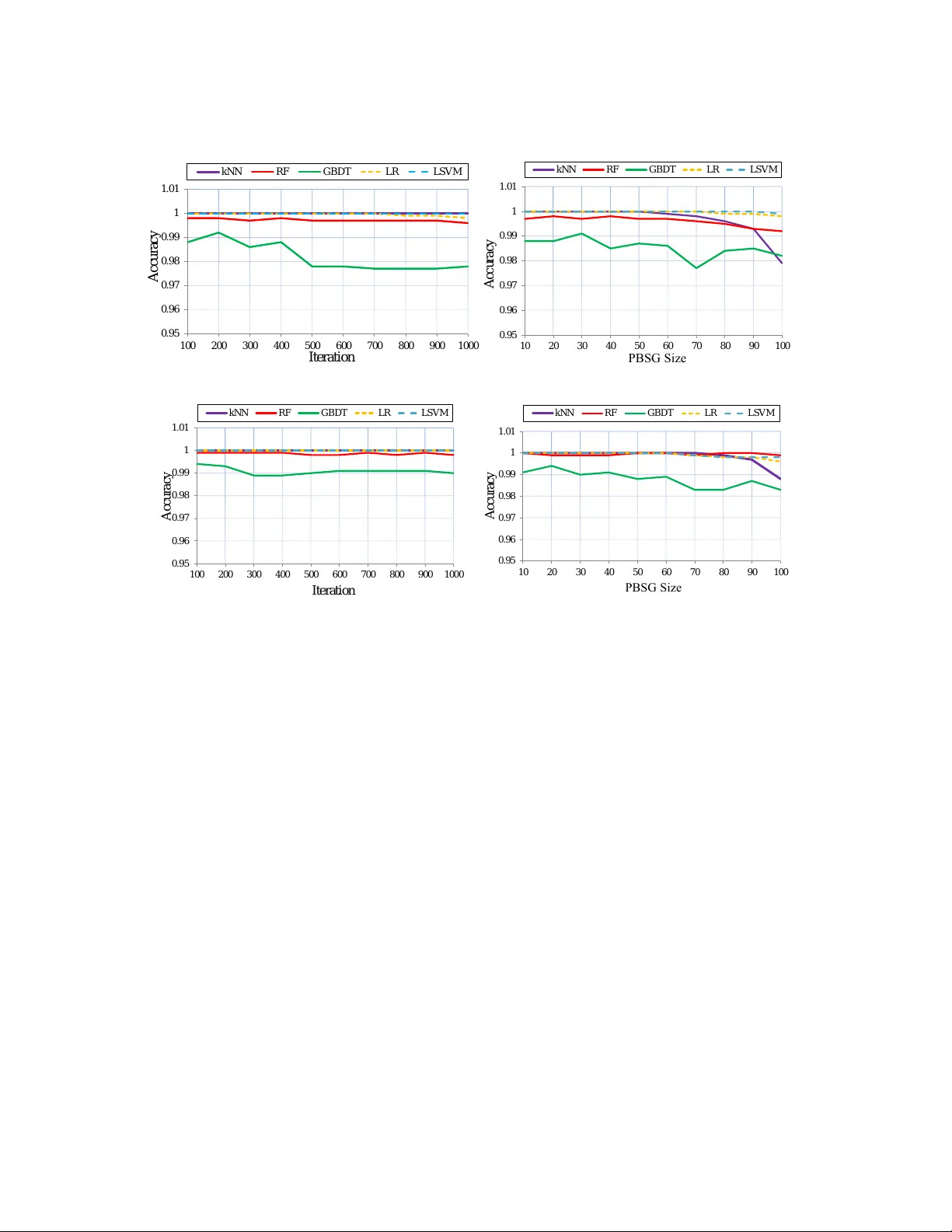
P ersistence B-Spline Grids: Stable V ector Represen tation of P ersistence Diagrams Based on Data Fitting Zhetong Dong ztdong@zju.edu.cn Hongw ei Lin ∗ hwlin@zju.edu.cn Chi Zhou elonzhou@zju.edu.cn Scho ol of Mathematic al Scienc es; State Key L ab. of CAD& CG, Zhejiang University, Hangzhou, Zhejiang Pr ovinc e, P.R.China Abstract Man y attempts hav e b een made in recen t decades to in tegrate machine learning (ML) and top ological data an alysis. A prominen t problem in applying p ersistent homology to ML tasks is ﬁnding a vector representation of a persistence diagram (PD), which is a summary diagram for represen ting top ological features. F rom the p ersp ectiv e of data ﬁtting, a stable v ector representation, namely , p ersistenc e B-spline grid (PBSG), is prop osed based on the eﬃcien t tec hnique of progressiv e-iterativ e appro ximation for least-squares B-spline function ﬁtting. W e theoretically pro ve that the PBSG metho d is stable with resp ect to the metric of 1-W asserstein distance deﬁned on the PD space. The prop osed metho d was tested on a syn thetic data set, data sets of randomly generated PDs, data of a dynamical system, and 3D CAD mo dels, showing its eﬀectiveness and eﬃciency . Keyw ords: P ersistent Homology , Mac hine Learning, Persistence Diagram, B-Spline F unction, Progressiv e-Iterative Approximation 1. In tro duction Inferring the top ological structures of data at diﬀerent scales is one ma jor task in the adv ent of the big-data era. Persistent homolo gy (Edelsbrunner et al., 2002; Zomorodian and Carlsson, 2005) pro vides a robust to ol to capture top ological features in data. These homological features in a dimension are summarized in a p ersistenc e diagr am (PD) or a b ar c o de (Ghrist, 2008). Persisten t homology has also b een applied successfully to deal with v arious practical problems in diﬀerent scien tiﬁc and engineering ﬁelds, such as bio c hemistry (Xia and W ei, 2015; Xia et al., 2018) and information science (De Silv a and Ghrist, 2007; Riec k et al., 2018). The mac hine learning (ML) comm unity has shown a growing interest in combining tra- ditional ML metho ds and the current tec hniques of computational topology (Chazal et al., 2015; Chen and Quadrian to, 2016; Khrulk ov and Oseledets, 2018). In ML applications, clas- siﬁcation tasks require comparing the similarit y b etw een tw o PDs. Therefore, the distance metrics of PDs, i.e., the W asserstein distance and the b ottleneck distance (Cohen-Steiner ∗ . Corresponding author © 2022 Zhetong Dong, Hongwei Lin and Chi Zhou. License: CC-BY 4.0, see https://creativecommons.org/licenses/by/4.0/ . Dong, Lin and Zhou et al., 2007), play an imp ortant role. Although some eﬃcient algorithms (Kerb er et al., 2017) were proposed to compute the distance metrics, it is limited to applying ML metho ds and statistics on the analysis of PDs. One of the alternatives is to extend the represen- tation of top ological features into the form of v ectors that ha ve the prop ert y of stabilit y with resp ect to the distance of PDs. A v ector represen tation has the adv an tages of easy distance computation and being a v ailable for more ML tools than distance matrix form. F or instance, a v ectorizing representation of PD is av ailable to supp ort vector machine (SVM), a commonly used ML to ol that requires v ectors as input. This con text, therefore, provides a clear motiv ation to represen t PDs by stable v ectors. 1.1 Related W ork Man y approac hes (Pac hauri et al., 2011; Carriere et al., 2015; Kali ˇ snik, 2018; Bubenik, 2015; Reininghaus et al., 2015; Adams et al., 2017; Chevyrev et al., 2020) ha ve b een pro- p osed to transform PDs into v ectors. Some attempts hav e b een dev elop ed when studying practical applications. F or example, while studying the cortical thickness measuremen ts of the h uman cortex for the study of Alzheimer’s disease, Pac hauri et al. (2011) rasterized PDs on a regular grid to v ectorize the concentration map for SVM training. Some studies (Di F abio and F erri, 2015; Adco ck et al., 2016; Kali ˇ snik, 2018) represented PDs b y using an algebraic p olynomial or function. F or example, Kali ˇ snik (2018) iden tiﬁed tropical co or- dinates on the barcode space and prov ed the stabilit y of this represen tation with respect to the barco de metrics. Some related studies (Mileyko et al., 2011) dev elop ed statistical measuremen ts of the PDs, suc h as p ersistence landscap es (Bubenik, 2015), the functional represen tation satisfying the prop osed ∞ -landscap e stability and p -landscap e stability with the same condition as the stability of the p -W asserstein distance (Cohen-Steiner et al., 2010). In this pap er, w e will compare the p erformance among our metho ds, p ersistence landscap es (PLs) (Bub enik, 2015), persistence images (PIs) (Adams et al., 2017), p ersis- tence scale space kernel (PSSK) (Reininghaus et al., 2015), p ersistence w eighted Gaussian k ernel (PWGK) (Kusano et al., 2018), sliced W asserstein k ernel (SWK) (Carriere et al., 2017), and p ersistence bag-of-words (PBoW) (Zieli ´ nski et al., 2019) in some ML classiﬁca- tion tasks. Therefore, the related works on these comp etitive metho ds are review ed. P ersistence images : PIs prop osed by Adams et al. (2017) combined the idea of the k ernel framew ork in Reininghaus et al. (2015) and the idea of “pixel” coun ting in Rouse et al. (2015). Sp eciﬁcally , the pro duct of a Gaussian distribution and a w eighted function corresp onding to eac h PD p oin t in the birth-p ersistence co ordinates are added up to form a p ersistence surface. By integrating the p ersistence surface on eac h pixel divided on the domain, a grayscale image is pro duced, which is often reshap ed to b e a vector. In particular, the Gaussian function tends to the Dirac delta if the v ariance σ approac hes zero, and PIs degenerate into the w eighted summation in Rouse et al. (2015). Among their adv antages, PIs allow users to assign a weigh t on each p oint in a PD, and provide an eﬃcient and easily understandable approach to vectorize PDs for ML tasks. Similar to the case of the k ernel in Reininghaus et al. (2015), PIs ha ve 1-W asserstein stability , and the p ersistence surface of a PI is additiv e, in tro ducing diﬃculties in pro ving the stabilit y results with respect to p -W asserstein distance when 1 < p ≤ ∞ . 2 Persistence B-Spline Grids: St able Vector Represent a tion of Persistence Diagrams Kernel metho ds : Kernel metho ds ha ve b een widely developed for ﬁnding an appro- priate measurement of PD distance. The main idea of the framework of k ernel metho ds is to transform PDs into probability density functions so that the distance b etw een the PDs can b e ev aluated. Inspired by a heat diﬀusion problem with a Dirichlet b oundary condi- tion, Reininghaus et al. (2015) prop osed the PSSK. PSSK is a framew ork of an additiv e m ulti-scale k ernel, and has 1-W asserstein stabilit y . Kusano et al. (2018) summarized pre- vious studies based on kernel functions and developed the PWGK that vectorizes PDs by using k ernel embedding of measures into reproducing kernel Hilbert spaces. The stabilit y of PW GK w as pro ved with resp ect to the Hausdorﬀ distance b et ween data. The SWK for PDs w as prop osed b y Carriere et al. (2017). The p oints on PDs are pro jected on a series of lines passing through the origin, and the slop es of these lines are adjusted. By SWK, the distance of PDs is measured as the distances b etw een the pro jected p oints on these lines. SWK is a negativ e semi-deﬁnite kernel, and it has 1-W asserstein stabilit y . F urthermore, other kernel metho ds (Le and Y amada, 2018; Padellini and Brutti, 2017; Carri` ere and Bauer, 2019) are b eing developed to b e incorp orated into k ernel-based ML mo dels. P ersistence bag-of-words : Considering the considerable time consumption of kernel metho ds in practice caused b y explicit computation of k ernel matrix, Zieli´ nski et al. (2019) prop osed PBoW to transform a PD in to a ﬁnite-dimension v ector. This method extends the con ven tional bag-of-w ords to deal with PDs. The co deb o ok, a ﬁnite-size represe n tation, is generated b y conducting clustering and obtaining the cen ters of clusters on the diagram in to whic h all PDs of training samples are consolidated. The v ector represen tation is pro duced b y coun ting the num b er of p oints closest to the co deword in the co deb o ok in a given order. In a mild condition, the authors ga ve a stable form of PBoW that has 1-W asserstein stability . Ho wev er, the obtained v ectorizing representation via PBoW dep ends on the training samples and the clustering metho ds. 1.2 Con tributions of the Present Study F rom the p ersp ective of data ﬁtting and appro ximation, the weigh ted kernel framework can b e thought to interpolate with basis functions the “imp ortance” v alues. T o transform a PD into an explicit vector deriv ed from a B-spline con trol grid, we prop osed a data ﬁtting framew ork based on the persistence B-spline function that appro ximates the “imp ortance” v alues, named eminenc e functions . The information of PDs is enco ded in to the ﬁnitely dimensional vectors pro duced by the control grid of the function, so that one can reconstruct precisely the p ersistence surface from the vectors. Notably , while in PI (Adams et al., 2017), the p ersistence surface is discretized in to pixels to generate the v ectors. Then, some information is “lost” during the discretization. The v ectors pro duced by our metho d preserv e the whole information of the p ersistence B-spline function, thereb y improving eﬀectiv eness and eﬃciency . T o eﬃcien tly compute the persistence B-spline function, the tec hnique of pr o gr essive- iter ative appr oximation for le ast squar es B-spline function ﬁtting (LSPIA) (Deng and Lin, 2014) is used to robustly generate the v ectors. W e also prov ed that the v ectorizing repre- sen tations hav e stability with resp ect to the 1-W asserstein distance under some conditions. Generally , the prop osed framework for PD representation is (1) stable with resp ect to the W asserstein distance in diﬀeren t c hoices of eminence v alues, (2) eﬃcien t to compute 3 Dong, Lin and Zhou the control grid to form the vector, and (3) ﬂexible to select the “imp ortance” v alues (lo cal eminence v alues and global eminence v alues) for diﬀeren t practical tasks. 2. Bac kground In this section, w e provide brief in tro ductions on B-spline function and p ersistent ho- mology , related to the core concepts of the prop osed metho d. 2.1 B-Spline F unction First, B-spline is brieﬂy in tro duced, and readers can refer to Piegl and Tiller (2012) for details. A B-spline of order n is a piecewise p olynomial function of degree n − 1 with a v ariable t . A series of non-decreasing sequence {· · · ξ i − 1 , ξ i , ξ i +1 , · · · } denotes knots at whic h the pieces of p olynomials join. Given a sequence of knots, the B-splines of order 1 are deﬁned b y B i, 1 ( t ) = ( 1 , ξ i ≤ t < ξ i +1 , 0 , otherwise . (1) The B-splines of k th-order are deﬁned in the wa y of recursion b y B i,k ( t ) = t − ξ i ξ i + k − 1 − ξ i B i,k − 1 ( t ) + ξ i + k − t ξ i + k − ξ i + k − 1 B i +1 ,k − 1 ( t ) , (2) and thereb y , n th-order B-spline dep ends on ( k − 1)-th B-spline. The B-spline has the w eight prop ert y , i.e. , P i B i,n ( t ) = 1, for all n ≥ 1. Moreo ver, the con tinuit y of B i,n ( t ) dep ends on the order n and the multiplication. Sp eciﬁcally , for a B-spline basis function of order n , if r knots are coinciden t, then the ﬁrst n − r − 1 deriv ativ es of B i,n ( t ) are con tinuous across that knot. If the knots are distinct, then the ﬁrst n − 2 deriv atives are con tinuous across eac h knot. And if the distance b et ween eac h knot and its predecessor, i.e. , ξ i +1 − ξ i , is the same, the knot vector and the corresp onding B-splines are called uniform . A ( p, q )-order uniform B-spline function , of whic h the degree is ( p − 1 , q − 1), is deﬁned b y S ( s, t ) = h X i =1 h X j =1 P ij B i,p ( s ) B j,q ( t ) s, t ∈ [0 , 1] (3) where { P ij } ’s are the c ontr ol p oints in the space with the size h × h , and the p th-order B-spline basis B i,p ( s ) and q th-order B-spline basis B j,q ( t ) are deﬁned, resp ectively , on the knot sequences on [0 , 1] S = { 0 , · · · , 0 | {z } p , ξ s 1 , · · · , ξ s h − p , 1 , · · · , 1 | {z } p } T = { 0 , · · · , 0 | {z } q , ξ t 1 , · · · , ξ t h − q , 1 , · · · , 1 | {z } q } , whic h mak es the prop erty of endp oin t in terp olation hold. Note that, in our implementation, the bi-cubic uniform B-spline function, i.e. , p = q = 4, is used for data ﬁtting. 4 Persistence B-Spline Grids: St able Vector Represent a tion of Persistence Diagrams 2.2 P ersistent Homology P ersistent homology (Edelsbrunner and Harer, 2010; Edelsbrunner et al., 2002) aims to infer the topological structures of the underlying shape from a p oint cloud sampled from it. P ersistent homology is based on formalism in algebraic top ology , namely , homol- ogy (Hatc her, 2002; Kaczynski et al., 2006), whic h describ es the “holes” with dimensions of a top ological space in the language of algebra. In tuitively , a homology class in the k -th homology group of a top ological space represents a k -dimensional “hole”. T o in tro duce the concept of PD, we in tuitively explain the ﬁltration based on the Vietoris-Rips (V-R) com- plex, the meaning of PDs, and the stability theorems of PD. The textb o ok (Edelsbrunner and Harer, 2010) provides further information. Let X = { p 1 , · · · , p n } b e a ﬁnite p oint set sampled from a shap e in a metric space with the metric d . A ball with its center p i and radius r is denoted as B ( p i , r ) = { x : d ( x , p i ) ≤ r } , i = 1 , · · · , n . F or a ﬁxed r ≥ 0, a k -simplex is deﬁned as a subset τ = { p i 0 , · · · , p i k } of X whic h satisﬁes that the balls of any tw o p oints intersect, i.e. , B ( p i j 1 , r ) ∩ B ( p i j 2 , r ) 6 = ∅ for an y p i j 1 , p i j 2 ∈ τ . The set of these simplexes with diﬀerent dimensions forms a simplicial complex, called the V-R complex of X with radius parameter r , denoted as V R ( X , r ). F or radius parameters r j 1 ≤ r j 2 , V R ( X , r j 1 ) is a sub complex of V R ( X , r j 2 ), and a nested sequence of simplicial complexes F ( X ) = { V R ( X , r j ) | r j ≥ 0 } is obtained, called a V-R complex ﬁltr ation . As parameter r increases, some homological inv arian ts emerge, and some disapp ear b e- cause of the app earance of simplexes. Mathematically , for r j 1 ≤ r j 2 , the inclusion b etw een V R ( X , r j 1 ) and V R ( X , r j 2 ) induces a homomorphism κ r j 2 r j 1 from the k -th homology group H k ( V R ( X , r j 1 )) to H k ( V R ( X , r j 2 )). The k -th persistent homology of the ﬁltration F ( X ) is deﬁned b y the collection of homology groups and the induced homomorphisms, specif- ically demonstrated in Zomoro dian and Carlsson (2005). In tuitively , a k -th homological class is b orn at r j 1 if it emerges in H k ( V R ( X , r j 1 )), and it dies at r j 2 if it disapp ears in H k ( V R ( X , r j 2 )). Its lifetime r j 2 − r j 1 is called the p ersistenc e of the homological class. A k -th PD is a m ulti-set of tw o-dimensional p oin ts P D k = { ( x i , y i ) | i ∈ I } that summarizes the birth-death pairs ( x i , y i ) = ( r j 1 , r j 2 ) of the k -th homological class. On the tame condi- tion in Zomoro dian and Carlsson (2005), we can assume that all PDs hav e ﬁnite cardinality | I | < ∞ . T o measure the similarity of t wo k -th PDs denoted as P D (1) and P D (2) , distance metrics are introduced. Let ∆ = { ( x, x ) | x ≥ 0 } b e the diagonal p oint set with inﬁnite multiplicit y , and b : P D (1) ∪ ∆ → P D (2) ∪ ∆ b e a bijection. The b ottleneck distance b et ween tw o PDs is deﬁned b y W ∞ ( P D (1) , P D (2) ) = inf b sup P ∈ P D (1) ∪ ∆ k P − b ( P ) k ∞ , (4) and for 1 ≤ p ≤ ∞ , the p -W asserstein distance is deﬁned by W p ( P D (1) , P D (2) ) = inf b   X P ∈ P D (1) ∪ ∆ k P − b ( P ) k p ∞   1 /p , (5) where b ranges ov er all bijections from P D (1) ∪ ∆ to P D (2) ∪ ∆. One of the most imp ortant prop erties of PDs is that the transformation from data to a PD is contin uous with resp ect 5 Dong, Lin and Zhou to the distance metrics. As pro ved in Cohen-Steiner et al. (2007); Chazal et al. (2014), the b ottlenec k distance b etw een t w o k -th PDs from point sets X and Y is controlled by the Hausdorﬀ distance d H , that is, W ∞ ( P D k ( X ) , P D k ( Y )) ≤ d H ( X , Y ). The stability theorems with respect to p -W asserstein distance are prov ed on some conditions of the underlying space, provided in Cohen-Steiner et al. (2010). 3. Metho d and Algorithm In this section, w e propose a metho d for transforming a PD in to a ﬁnite-dimensional v ector. As illustrated in Fig. 1, PD p oin ts are transformed from the birth-death co ordinate to the birth-p ersistence coordinate and normalized. Then, an eminenc e value is assigned to eac h transformed 2D p oint. Subsequen tly , the eminence v alues are ﬁtted by a uniform bi-cubic B-spline function. Finally , a ﬁnite-dimensional vector is obtained by concatenating the control grid of the B-spline function. 1 0.8 0.6 0.4 0.2 0 Figure 1: The pipeline of transforming a PD into a v ector based on B-spline function ﬁtting. A PD with a certain dimension k is a multi-set ab o ve the diagonal, i.e. , P D = { ( x l , y l ) ∈ R 2 | y l > x l , l ∈ I } , (6) where I = { 1 , 2 , · · · , M } is an index set. T o presen t our metho d, some assumptions should b e made as follows: 6 Persistence B-Spline Grids: St able Vector Represent a tion of Persistence Diagrams Assumption 1 (1) Al l PDs we c onsider e d c ontain a ﬁnite numb er of p oints over the diagonal, i.e., | I | < ∞ ; (2) Al l p oints in al l PDs ar e b ounde d, 1 and denote m as the maximum of the diﬀer enc e b etwe en upp er and lower b ounds of the birth c o or dinates and the p ersistenc e, i.e., letting x min = min l ∈ I ( x l ) and x max = max l ∈ I ( x l ) , m = max  x max − x min , max l ∈ I ( y l − x l )  < ∞ . These assumptions are based on the theory of a tame persistent homology in tro duced in Section 2.2 and practical observ ation. This section is organized as follows. In Section 3.1, the co ordinate transformation and eminence function are in tro duced. In Section 3.2, the p ersistence B-spline grid, the k ey con- cept of our framework, is deﬁned. In Section 3.3, the algorithm based on the approximation tec hnique LSPIA is summarized for the v ectorization of PDs. 3.1 Co ordinate T ransformation and Eminence F unctions As the transformation adopted in Adams et al. (2017), PDs are transformed in to the birth-p ersistence co ordinates and normalized into a unit region. According to Assumption 1, m is the maximum of the diﬀerence b etw een upp er and lo wer b ounds of the birth coordinates and the p ersistence in all PDs we considered, and the lo wer b ound of the birth co ordinates in all PDs is denoted as c . 2 The co ordinate transformation φ : R 2 → [0 , 1] 2 is deﬁned b y φ ( x, y ) = (( x − c ) /m, ( y − x ) /m ) , ( s, t ) . (7) The normalized birth-p ersistence co ordinate is denoted by ( s l , t l ) = φ ( x l , y l ) for ( x l , y l ) ∈ P D (6). T o measure the signiﬁcance of a birth-death pair in a PD, an eminenc e value is assigned to each pair by deﬁning diﬀeren t eminence functions. The principles of designing an em- inence function dep end on the understanding of diﬀeren t p ersistence in a practical task. Generally , the birth-death pair close to the diagonal is thought to be noise and marked with a small eminence v alue. By con trast, the pair with large p ersistence is marked with a large eminence v alue. Therefore, to design the eminence function, w e prop ose t wo alternativ es, namely , lo c al eminenc e function and glob al eminenc e function . Lo cal Eminence F unction : Given a birth-death pair ( x, y ), the lo cal eminence func- tion assigns to eac h PD p oint a lo c al eminenc e value that dep ends only on its p ersistence w = y − x . T o make the stability hold in Section 4, the univ ariate lo cal eminence function E L : R → R E L,P D ( x, y ) , E L ( y − x ) = E L ( w ) , (8) should satisfy the following conditions: 1. Reduced 0-th PD is used to ov ercome the emergence of an inﬁnitely p ersistent feature. 2. In particular, in classiﬁcation tasks, m and c depend on the PDs of training data. F or the test data, the PDs are truncated by m and c . 7 Dong, Lin and Zhou (1) E L ( w ) is a monotonically increasing function, i.e. , if w 1 < w 2 , then E L ( w 1 ) ≤ E L ( w 2 ); (2) E L ( w ) is a b ounded and diﬀeren tiable function with its ﬁrst-order deriv ative b ounded, i.e. , kE L k ∞ < ∞ and sup w ∈ R |E 0 L ( w ) | < ∞ . Global Eminence F unction : T o consider p ersistence of a PD p oint and the distribu- tion of all p oin ts on a PD, the global eminence function assigns a glob al eminenc e value to a PD point. Given a PD, the global eminence function has the form E G,P D ( x, y ) = X l ∈ I ( y l − x l ) K ( x − x l , y − y l ) , (9) where K ( x, y ) is a basis function and ( x l , y l ) ∈ P D . F or stabilit y in Section 4, the global eminence function is supp osed to follo w the principles: (1) the basis function K ( x, y ) is b ounded and diﬀeren tiable, i.e. , kK ( x, y ) k ∞ < ∞ ; (2) the ﬁrst-order partial deriv ativ es of K ( x, y ) with resp ect to x and y are b ounded, i.e. , sup ( x,y ) ∈ R 2 k∇K ( x, y ) k 2 < ∞ . 3.2 P ersistence B-Spline Grid F or each transformed co ordinate ( s l , t l ) in a PD, an eminence v alue z l is assigned through a lo cal eminence function, i.e ., z l = E L,P D ( x, y ) = E L ( y l − x l ) , (10) or through a global eminence function, i.e. , z l = E G,P D ( x l , y l ) . (11) Then, the eminence v alues are ﬁtted by a uniform bi-cubic B-spline function with h × h size of the con trol p oints as follows: S ( s, t ) = h X i =1 h X j =1 e z ij B i ( s ) B j ( t ) , (12) where h is the grid size satisfying h ≥ 4, and the uniform cubic B-spline basis B i ( s ) and B j ( t ) are both deﬁned on the uniform knot sequence ξ =  0 , 0 , 0 , 0 , 1 h − 3 , · · · , h − 4 h − 3 , 1 , 1 , 1 , 1  . (13) T o obtain the uniform bi-cubic B-spline function (12) that ﬁts the eminence v alues, the follo wing least-squares problem should b e solved: min { e z ij } X l ∈ I k z l − S ( s l , t l ) k 2 2 . (14) 8 Persistence B-Spline Grids: St able Vector Represent a tion of Persistence Diagrams It is equiv alent to solving the normal equation, B T B e Z = B T Z , (15) where e Z = ( e z 11 , e z 12 , · · · , e z 1 h , e z 21 , e z 22 , · · · , e z 2 h , · · · , e z h 1 , e z h 2 , · · · , e z hh ) T , (16) Z = ( z 1 , z 2 , · · · , z M ) T , (17) and the matrix B is the collo cation matrix of the B-spline basis at { ( s l , t l ) | l ∈ I } . By arranging the B-spline basis in a vector and denoting B i ( s ) B j ( t ) as B ( i − 1) × h + j ( s, t ), i.e. , [ B 1 ( s ) B 1 ( t ) , B 1 ( s ) B 2 ( t ) , · · · , B 1 ( s ) B h ( t ) , B 2 ( s ) B 1 ( t ) , · · · , B 2 ( s ) B h ( t ) , · · · , B h ( s ) B 1 ( t ) , · · · , B h ( s ) B h ( t )] , [ B 1 ( s, t ) , B 2 ( s, t ) , · · · , B h 2 ( s, t )] , the collo cation matrix B at { ( s l , t l ) , l ∈ I } can b e written as B =         B 1 ( s 1 , t 1 ) B 2 ( s 1 , t 1 ) B 3 ( s 1 , t 1 ) · · · B h 2 ( s 1 , t 1 ) B 1 ( s 2 , t 2 ) B 2 ( s 2 , t 2 ) B 3 ( s 2 , t 2 ) · · · B h 2 ( s 2 , t 2 ) . . . . . . . . . · · · . . . . . . . . . . . . · · · . . . B 1 ( s M , t M ) B 2 ( s M , t M ) B 3 ( s M , t M ) · · · B h 2 ( s M , t M )         . (18) W e deﬁne some terminologies as follows. Deﬁnition 1 (P ersistence B-spline function, PBSG, and vector of PBSG) (1) The uniform bi-cubic B-spline function (12) which ﬁts the eminenc e values is c al le d the p ersistence B-spline function . (2) The c ontr ol grid of the p ersistenc e B-spline function (12) is c al le d the p ersistence B-spline grid (PBSG) . (3) The ve ctor e Z gener ate d by arr anging PBSG with the lexic o gr aphic or der, shown in (16) , is c al le d the v ector of PBSG . In the persistence B-spline function (12), the size of its control grid (PBSG) is h × h . W e call h or h × h the size of the PBSG . Deﬁnition 2 (Lo cal eminence v ector and global eminence vector) (1) The ve ctor Z (17) is c al le d a lo cal eminence vector , if its elements ar e taken fr om a lo c al eminenc e function by Eq. (10) . (2) The ve ctor Z (17) is c al le d a global eminence v ector , if its elements ar e taken fr om a glob al eminenc e function by Eq. (11) . The lo c al and glob al eminenc e ve ctors ar e b oth c al le d eminence vectors . If a PBSG is generated by ﬁtting a lo cal eminence vector, we call it a lo c al PBSG . Similarly , if a PBSG is pro duced b y ﬁtting a global eminence vector, we call it a glob al PBSG . 9 Dong, Lin and Zhou 3.3 Algorithm for PBSG As stated to obtain the solution of the least-squares ﬁtting problem (14), the normal equation (15) should b e solv ed. How ev er, the co eﬃcient matrix of the normal equation (15) can b e either non-singular or singular. When it is singular or near singular, special treatmen ts should b e used to obtain a robust solution. In this article, we use LSPIA (Deng and Lin, 2014; Lin et al., 2018) to eﬀectiv ely and eﬃcien tly solve the linear system (15). Regardless of whether the co eﬃcient matrix is singular, LSPIA can conv erge to the solu- tion of the linear system (15) in a uniﬁed format, without any sp ecial treatmen t. When the co eﬃcient matrix is singular, an inﬁnite n umber of solutions are p ossible, and LSPIA con verges to the solution with minimum Euclidean norm (Lin et al., 2018). LSPIA b egins with an initial B-spline function S (0) ( s, t ) = h X i =1 h X j =1 e z (0) ij B i ( s ) B j ( t ) s, t ∈ [0 , 1] , (19) where the initial con trol points are all zero, i.e. , e z (0) ij = 0. Let δ (0) l = z l − S (0) ( s l , t l ) b e the diﬀerence b etw een the eminence v alues (10)(11) and the corresp onding v alues S (0) ( s l , t l ) on the function S (0) , and tak e the initial diﬀerences for the control p oin ts as ∆ (0) ij = 1 C M X l =1 B i ( s l ) B j ( t l ) δ (0) l , (20) where the setting of the parameter C is discussed later. Then, adding the diﬀerence for the con trol points (20) to the control p oin ts e z (0) ij , we obtain the new con trol p oin ts e z (1) ij = e z (0) ij + ∆ (0) ij , whic h then generate a new function S (1) ( s, t ). Supp os e that the k -th function S ( k ) ( s l , t l ) is obtained. W e calculate δ ( k ) l = z l − S ( k ) ( s l , t l ) , ∆ ( k ) ij = 1 C M X l =1 B i ( s l ) B j ( t l ) δ ( k ) l , e z ( k +1) ij = e z ( k ) ij + ∆ ( k ) ij , (21) and the ( k + 1)st B-spline function is generated as S ( k +1) ( s, t ) = h X i =1 h X j =1 e z ( k +1) ij B i ( s ) B j ( t ) s, t ∈ [0 , 1] . (22) In general, the iteration will stop when the giv en iteration time N is reached, or the diﬀer- ence error is less than a threshold ε , i.e. ,       1 √ M   v u u t M X l =1 ( δ ( k − 1) l ) 2 − v u u t M X l =1 ( δ ( k ) l ) 2         < ε. 10 Persistence B-Spline Grids: St able Vector Represent a tion of Persistence Diagrams F or the conv enience to show the stabilit y of PBSGs in Section 4, we set a maximum iteration time N to stop the LSPIA iteration. The parameter C in (20) and (21) is a p ositiv e constan t. If C ≥ k B T k ∞ = max 1 ≤ i,j ≤ h ( M X l =1 B i ( s l ) B j ( t l ) ) , (23) the LSPIA algorithm conv erges (Lin and Zhang, 2013; Deng and Lin, 2014; Lin et al., 2018). In our implemen tation, we set C = max 1 ≤ i,j ≤ h n P M l =1 B i ( s l ) B j ( t l ) o to sp eed up the con vergence rate of LSPIA. Based on the result of conv ergence of a general LSPIA format, the conv ergence of this algorithm is prov ed in App endix 8. Finally , w e summarize the algorithm to compute the PBSG by LSPIA in Algorithm 1. Algorithm 1: Compute PBSG by LSPIA. Input: A PD represented b y a m ultiset { ( x l , y l ) } M l =1 , the maxim um iteration time N , the maxim um v alue m and the lo wer b ound c in (7), and the lo cal/global eminence function. Compute transformed co ordinates ( s l , t l ) = φ ( x l , y l ) , l = 1 , 2 · · · , M b y (7); Compute eminence v alues z l , l = 1 , 2 , · · · , M (10)(11); e z (0) ij = 0 , 1 ≤ i, j ≤ h ; for k = 0 ; k ≤ N ; k = k + 1 do S ( k ) ( s l , t l ) = P h i =1 P h j =1 e z ( k ) ij B i ( s l ) B j ( t l ); δ ( k ) l = z l − S ( k ) ( s l , t l ), for l = 1 , 2 , · · · , M ; ∆ ( k ) ij = 1 C P M l =1 B i ( s l ) B j ( t l ) δ ( k ) l ; e z ( k +1) ij = e z ( k ) ij + ∆ ( k ) ij ; end Concatenate e z ( N ) ij in to a vector e Z (16) lexicographically . Output: the v ector of PBSG e Z . 4. Stabilit y of V ectorizing Represen tation In this section, w e pro ve the stability of PBSG with resp ect to 1-W asserstein distance b et ween PDs by the following steps: (1) W e ﬁrst show the stabilit y of lo cal and global eminence v alues and the transformed co ordinates. (2) A core lemma on the LSPIA iteration metho d is sho wn to bridge the vectors of eminence v alues, transformed co ordinates, and PBSG. (3) The stability of lo cal and global PBSG is induced. 11 Dong, Lin and Zhou Let P D (1) = n P (1) l = ( x (1) l , y (1) l ) o M l =1 b e a given PD and P D (2) = n P (2) l = ( x (2) l , y (2) l ) o M l =1 b e the p erturb ed PD, resp ectiv ely . In the 1-W asserstein distance betw een these t wo PDs, the mapping b is the matc hing bijection that achiev es the inﬁm um, satisfying, P (2) l = b ( P (1) l )) , l = 1 , 2 , · · · , M . Therefore, we ha ve, W 1 ( P D (1) , P D (2) ) = M X l =1    P (1) l − b ( P (1) l )    ∞ = M X l =1    P (1) l − P (2) l    ∞ . In addition, the ve ctors of tr ansforme d c o or dinates from P D ( i ) , i = 1 , 2, giv en by (7), are denoted as, u ( i ) =  s ( i ) 1 , · · · , s ( i ) l , · · · , s ( i ) M , t ( i ) 1 , · · · , t ( i ) l , · · · , t ( i ) M  , i = 1 , 2 , resp ectiv ely . The eminenc e ve ctors of P D ( i ) , given b y (17), are denoted as Z ( i ) , i = 1 , 2, respectively . And the ve ctors of PBSG (16) generated from P D ( i ) are represen ted b y e Z ( i ) , i = 1 , 2, resp ectively . T o prov e the stabilit y of PBSG, w e use the assumptions men tioned in Section 3 (Assumption 1). 4.1 Stabilit y of Eminence V alues and T ransformed Co ordinates Stabilit y of lo cal eminence v alues : In the case that the eminence v alues are assigned via a lo cal eminence function (8), the eminence v alue is determined only by the p ersistence of the PD p oin t. Thus, w e ha ve z l = E L,P D ( x l , y l ) = E L ( y l − x l ). The follo wing lemma sho ws that the diﬀerence b etw een the lo cal eminence v ectors, i.e. , Z (1) and Z (2) , is con trolled by the multiplication of the 1-W asserstein distance b et ween P D ( i ) , i = 1 , 2 and a constan t. Lemma 3 Supp ose d that the lo c al eminenc e function E L (8) is diﬀer entiable and has a b ounde d ﬁrst-or der derivative, i.e., sup x ∈ R |E 0 L ( x ) | < ∞ , we have    Z (2) − Z (1)    1 ≤ 2 sup |E 0 L | W 1 ( P D (1) , P D (2) ) , (24) wher e sup |E 0 L | denotes sup x ∈ R |E 0 L ( x ) | . Pro of It follo ws b y using Lemma 9 in App endix 7 that for 1 ≤ l ≤ M ,    z (2) l − z (1) l    =    E L ( y (2) l − x (2) l ) − E L ( y (1) l − x (1) l )    ≤ sup x ∈ R |E 0 L ( x ) |    ( y (2) l − x (2) l ) − ( y (1) l − x (1) l )    = sup |E 0 L |    ( y (2) l − y (1) l ) − ( x (2) l − x (1) l )    , (25) where sup x ∈ R |E 0 L ( x ) | := sup |E 0 L | . Because for an y a, b ∈ R , | a − b | ≤ | a | + | b | ≤ 2 max {| a | , | b |} holds, we ha ve    z (2) l − z (1) l    ≤ 2 sup |E 0 L | max n | x (2) l − x (1) l | , | y (2) l − y (1) l | o = 2 sup |E 0 L |    P (1) l − P (2) l    ∞ , (26) 12 Persistence B-Spline Grids: St able Vector Represent a tion of Persistence Diagrams where P (1) l =  x (1) l , y (1) l  and P (2) l =  x (2) l , y (2) l  . Consider the diﬀerence of Z (1) and Z (2) measured by 1-norm, and it ﬁnally holds that    Z (1) − Z (2)    1 ≤ 2 sup |E 0 L | M X l =1    P (1) l − P (2) l    ∞ = 2 sup |E 0 L | W 1 ( P D (1) , P D (2) ) . (27) Stabilit y of global eminence v alues : F or a global eminence function determined by all p oints in a PD, as shown in (9), the following lemma sho ws that the diﬀerence of the global eminence v ectors under 1-norm, i.e. ,   Z (1) − Z (2)   1 , is controll ed b y the multiplica- tion of the 1-W asserstein distance b etw een P D ( i ) , i = 1 , 2 and a constan t. Lemma 4 Supp ose d that b asis function K ( x, y ) of the glob al eminenc e function in (9) is b ounde d and diﬀer entiable with b ounde d ﬁrst-or der p artial derivatives, we have    Z (1) − Z (2)    1 ≤ 2 M (2 m sup k∇K k 2 + kK k ∞ ) W 1 ( P D (1) , P D (2) ) , (28) wher e kKk ∞ = max ( x,y ) ∈ R 2 |K ( x, y ) | , sup k∇Kk 2 = sup ( x,y ) ∈ R 2 k∇Kk 2 , and m is given in As- sumption 1. The pro of of Lemma 4 is attached in App endix 7. Stabilit y of co ordinate transformation : Recall that birth-death co ordinates are transformed to the birth-p ersistence co ordinates through (7). In the following lemma, w e sho w that the v ector of the transformed co ordinates is stable with resp ect to the 1- W asserstein distance b et ween PDs. Sp eciﬁcally , the diﬀerence b etw een the vectors of the transformed co ordinates under 1-norm is con trolled b y the m ultiplication of the 1- W asserstein distance b etw een P D ( i ) , i = 1 , 2 and a constan t. Lemma 5 F or the ve ctors of tr ansforme d c o or dinates u ( i ) fr om P D ( i ) , i = 1 , 2 , thr ough the tr ansformation in (7) , we have    u (1) − u (2)    1 ≤ 4 m W 1 ( P D (1) , P D (2) ) , (29) wher e m is given in Assumption 1. Pro of Recall (7) that s l = ( x l − c ) /m, t l = ( y l − x l ) /m , for 1 ≤ l ≤ M . Th us, w e hav e    u (1) − u (2)    1 = M X l =1    s (1) l − s (2) l    + M X l =1    t (1) l − t (2) l    = 1 m " M X l =1    x (1) l − x (2) l    + M X l =1    ( y (1) l − x (1) l ) − ( y (2) l − x (2) l )    # = 1 m " M X l =1    x (1) l − x (2) l    + M X l =1    ( y (1) l − y (2) l ) − ( x (1) l − x (2) l )    # . (30) 13 Dong, Lin and Zhou It follows b y the inequit y | a − b | ≤ | a | + | b | ≤ 2 max {| a | , | b |} , for any a, b ∈ R that    u (1) − u (2)    1 ≤ 1 m M X l =1    x (1) l − x (2) l    + M X l =1    y (1) l − y (2) l    +    x (1) l − x (2) l    ! ≤ 2 m M X l =1     y (1) l − y (2) l    +    x (1) l − x (2) l     ≤ 4 m M X l =1 max n    y (1) l − y (2) l    ,    x (1) l − x (2) l    o . (31) Let P (1) l =  x (1) l , y (1) l  and P (2) l =  x (2) l , y (2) l  . It ﬁnally holds that    u (1) − u (2)    1 ≤ 4 m M X l =1    P (1) l − P (2) l    ∞ = 4 m W 1 ( P D (1) , P D (2) ) . (32) 4.2 Stabilit y on LSPIA In this section, w e pro vide a lemma based on the matrix form of LSPIA w hen the iteration time N is ﬁnite. The LSPIA iterativ e format shown in (21) can b e rewritten in a matrix form, in tro duced in Lin et al. (2018), as follo ws: e Z ( k +1) = e Z ( k ) + ΛB T  Z − B e Z ( k )  e Z (0) = O , (33) where e Z ( k ) represen ts the vector of PBSG after k iterations of LSPIA, Λ = diag (1 /C, 1 /C, · · · , 1 /C ) is a diagonal matrix, C is an iterativ e parameter (a constant), Z is the eminence vector given in (16), B is the collo cation matrix sho wn in (18), and O is a zero v ector. The iterative format in (33) is equiv alen t to e Z ( k +1) =  E − ΛB T B  e Z ( k ) + ΛB T Z , (34) where E is an identit y matrix. In the following, w e will estimate the diﬀerence b et ween the v ectors of PBSG e Z ( i ) ( k +1) from P D ( i ) , i = 1 , 2, under 2-norm after k + 1 iterations of LSPIA. Lemma 6 L et B ( i ) b e the c ol lo c ation matric es (18) at the tr ansforme d c o or dinate u ( i ) , i = 1 , 2 , r esp e ctively. F or the ve ctors of PBSG e Z ( i ) ( k +1) fr om P D ( i ) , i = 1 , 2 , after k + 1 iter ations of LSPIA, we have    e Z (1) ( k +1) − e Z (2) ( k +1)    2 ≤ √ 2 αh ( k +1)(2 hk M √ C 3 + √ M C ) kE k ∞    u (1) − u (2)    2 + k + 1 √ C    Z (1) − Z (2)    2 , (35) 14 Persistence B-Spline Grids: St able Vector Represent a tion of Persistence Diagrams wher e α = 2( h − 3) is the b ound of | B 0 i ( s ) | given in L emma 12, h is the size of PBSG, C is the iter ative p ar ameter given in (23) , and E r epr esents the lo c al eminenc e function E L,P D (8) or glob al eminenc e function E G,P D (9) . The pro of of Lemma 6 is provided in App endix 7. 4.3 Stabilit y of PBSG In this section, by using the lemmas pro v ed ab o ve, we pro vide stability results of the v ector of lo cal and global PBSG based on a ﬁnite iterations N of LSPIA. The following theorem shows that the vector of lo cal PBSG is stable with resp ect to the 1-W asserstein distance b etw een PDs. Theorem 7 (Stabilit y for Lo cal Eminence F unction) Assume that the iter ative p a- r ameter C satisﬁes (23) and C ≥ M . F or the lo c al eminenc e ve ctors Z ( i ) , pr o duc e d fr om a lo c al eminenc e function E L , and the ve ctors of PBSG e Z ( i ) ( N ) fr om P D ( i ) , i = 1 , 2 , we have    e Z (1) ( N ) − e Z (2) ( N )    2 ≤ C loc W 1 ( P D (1) , P D (2) ) , (36) wher e the stabilit y coeﬃcient C loc = 2 N √ C  2 √ 2 αh m (2 h ( N − 1) + 1) kE L k ∞ + sup |E 0 L |  , (37) in which α = 2( h − 3) is the b ound of | B 0 i ( s ) | in L emma 12, h is the size of PBSG, m is given in Assumption 1, and sup |E 0 L | = sup x ∈ R |E 0 L ( x ) | . Pro of Since C ≤ M , M /C ≤ 1. Due to (47) in Lemma 11, w e ha ve    u (1) − u (2)    2 ≤    u (1) − u (2)    1 , and    Z (1) − Z (2)    2 ≤    Z (1) − Z (2)    1 . By substituting (24) and (29) in to (35), (36) is obtained. Analogously , the following theorem sho ws that the vector of global PBSG is stable with resp ect to the 1-W asserstein distance b etw een PDs. Theorem 8 (Stabilit y for Global Eminence F unction) Assume that the iter ative p ar ameter C satisﬁes (23) and C ≥ M 2 . F or the glob al eminenc e ve ctors Z ( i ) , pr o duc e d fr om a glob al eminenc e function E G,P D ( x, y ) , and the ve ctors of PBSG e Z ( i ) ( N ) fr om P D ( i ) , i = 1 , 2 , we have    e Z (1) ( N ) − e Z (2) ( N )    2 ≤ C g lob W 1 ( P D (1) , P D (2) ) , (38) wher e the stabilit y coeﬃcient C g lob = 4 √ 2 αhN (2 h ( N − 1) + 1) kKk ∞ + 4 N m sup k∇K k 2 + 2 N kKk ∞ , (39) in which α = 2( h − 3) is the b ound of | B 0 i ( s ) | in L emma 12, h is the size of PBSG, m is given in Assumption 1, kK k ∞ = max ( x,y ) ∈ R 2 |K ( x, y ) | , and sup k∇K k 2 = sup ( x,y ) ∈ R 2 k∇Kk 2 . 15 Dong, Lin and Zhou Pro of Because C ≥ M 2 ≥ M when M ≥ 1, M /C ≤ 1 and M / √ C ≤ 1 hold. Note that kE G,P D k ∞ ≤ P M l =1 | y l − x l |kK ( x − x l , y − y l ) k ∞ ≤ P M l =1 m kKk ∞ = mM kKk ∞ . Due to (47) in Lemma 11, w e ha ve   u (1) − u (2)   2 ≤   u (1) − u (2)   1 , and   Z (1) − Z (2)   2 ≤   Z (1) − Z (2)   1 . By substituting (28) and (29) in to (35), (38) is obtained. Eqs. (37) and (39) explicitly giv e upper b ounds of the stabilit y co eﬃ cien ts C loc and C g lob . Ho wev er, it is diﬃcult to induce the theoretical supremum for the stability co eﬃcients. In Section 5.2, w e estimated the stability co eﬃcien ts b y computing    e Z (1) ( N ) − e Z (2) ( N )    2 /W 1 ( P D (1) , P D (2) ) , (40) using elab orately designed numerical examples. In all the numerical examples, the estima- tion (40) of the stability co eﬃcien ts are all less than 10 . 0. 5. Exp eriments This section is organized as follows. In Section 5.1, w e assessed the prop osed vectorizing represen tation with diﬀerent choices of parameters. In Section 5.2, w e estimated the upp er b ounds of the stability co eﬃcien ts on data sets of randomly generated PDs. In Section 5.3, w e compare the performance of our represen tation and other methods, namely PIs, PLs, SWK, PWGK, PSSK, PBoW, in classiﬁcation tasks to distinguish the dynamical systems and classify CAD mo dels. In Section 5.4, we explained the diﬀerences b etw een PI and our metho d, and conducted a comparison experiment to sho w the b etter p erformance of our metho d. In all exp erimen ts, the 0th or 1st PDs were computed by constructing the ﬁltration of V-R complexes of a p oint cloud in the space equipp ed with Euclidean metric b y using the Python pac k age Ripser (Bauer, 2017). In classiﬁcation tasks, ﬁve commonly used ML classiﬁers were used, namely , k -nearest neighbor classiﬁer ( k NN), random forest (RF) in Breiman (2001), gradient b o osted decision trees (GBDT) in F riedman (2001), logistic regression (LR), and linear supp ort vector mac hine (LSVM) in F an et al. (2008). All exp erimen ts were run on a PC with an Intel r Core(TM) i7-7700 CPU@3.60 GHz × 8. The data sets, MA TLAB, and Python source co de can b e found on https://github.com/ ZC119/PB . 5.1 Eﬀect of P arameter Choice in PBSG The vector of PBSG relies on m ultiple parameters, including the choice of eminence function and its parameter, the iteration time N of LSPIA, and the size of PBSG h . In this section, w e ev aluated the eﬀect of parameter choice of PBSG on a syn thetic data set con taining ﬁve categories, and measured the classiﬁcation accuracy as a quantitativ e index that indicates the inﬂuence of diﬀeren t c hoices of parameters. As illustrated in Figure 2, the data set con tains a circle with radius 0 . 4; t wo concen tric circles with radii 0 . 2 and 0 . 4, resp ectiv ely; tw o disjoin t circles each with radius 0 . 2; a cluster of p oints sampled at random in the unit square; and t wo clusters of p oin ts sampled at random s eparately in tw o squares with edge length 0 . 5. W e generated 50 images for eac h type, and sampled 1 , 000 p oin ts for eac h image. The sampled data w ere p erturb ed b y 16 Persistence B-Spline Grids: St able Vector Represent a tion of Persistence Diagrams adding Gaussian noises ( η = 0 . 025). F or each classiﬁer, data w ere split into 70% training set and 30% test set. After p erforming 100 trials, the av erage classiﬁcation accuracy w as computed. On eac h classiﬁer, cross-v alidation was used to select the optimal parameters of classiﬁers. − 0 . 4 − 0 . 2 0 . 0 0 . 2 0 . 4 − 0 . 4 − 0 . 2 0 . 0 0 . 2 0 . 4 − 0 . 4 − 0 . 2 0 . 0 0 . 2 0 . 4 − 0 . 4 − 0 . 2 0 . 0 0 . 2 0 . 4 − 0 . 4 − 0 . 2 0 . 0 0 . 2 0 . 4 − 0 . 4 − 0 . 2 0 . 0 0 . 2 0 . 4 − 0 . 6 − 0 . 4 − 0 . 2 0 . 0 0 . 2 0 . 4 0 . 6 − 0 . 6 − 0 . 4 − 0 . 2 0 . 0 0 . 2 0 . 4 0 . 6 − 0 . 4 − 0 . 2 0 . 0 0 . 2 0 . 4 − 0 . 4 − 0 . 2 0 . 0 0 . 2 0 . 4 Figure 2: The sampling p oints from ﬁv e classes of toy data: Each sample is p erturb ed b y a Gaussian noise with η = 0 . 025. T o measure the ﬁtting precision of the p ersistence B-spline function (12), we used the ro ot mean square (RMS) error as follows: ε RMS = s P n l =1 ( δ ( k ) l ) 2 n , (41) where n is the n umber of p oints in the giv en PD, and δ ( k ) l is presented in (21). Given a collection of PDs, the av erage RMS error and the maxim um RMS error w ere used to measure the ﬁtting precision on the collection of PDs. Choice of local eminence function : T o c ho ose a desirable loc al eminence function, w e tested several commonly used candidates, including the linear function E L,P D ( x, y ) = E L ( y − x ) = b ( y − x ), the ar ctan function E L ( y − x ) = arctan[ b ( y − x ) 2 ], the exp onential function E L ( y − x ) = e b ( y − x ) − 1, where b is a parameter, and the sigmoidal function E L,P D ( x, y ; b ) = 1 1 + e − ( y − x + b ) , (42) where the parameter b means a translation on the standard sigmoidal function. With the sigmoidal function, the eminence v alues of the PD p oints with relativ ely small and medium p ersistence v aried considerably lot, whereas the change of those with markedly large p ersistence w as insigniﬁcan t. Moreo v er, by using the sigmoidal function, the a verage classiﬁcation accuracy of ﬁv e classiﬁers w as higher than that of other candidates. Therefore, the sigmoidal function was selected as a lo cal eminence function. Choice of global eminence function : As sho wn in (9), the global eminence function relies on a basis function and the p ersistence of PD p oints. In our framework, we assume that a t wo-dimensional basis function is the multiplication of tw o one-dimensional basis functions, i.e. , K ( x, y ; a 1 , a 2 ) = ϕ ( x ; a 1 ) · ϕ ( y ; a 2 ), where a 1 and a 2 are tunable parame- ters. In the pretest, we set the parameters a 1 = a 2 . W e tested commonly employ ed basis functions, including the Gaussian basis function ϕ ( x ; a ) = e − ax 2 , m ultiquadric function ϕ ( x ; a ) = 1 + ax 2 , inv erse multiquadric function ϕ ( x ; a ) = 1 / √ 1 + ax 2 , and sinc-Gaussian 17 Dong, Lin and Zhou function in Zhang and Ma (2011) as follo ws: ϕ ( x ; a ) =    sin( π x ) π x e − ax 2 , x 6 = 0 , 1 , x = 0 , (43) where a is a tunable parameter. Through the pretest, the v ectors of PBSG with the sinc- Gaussian function as a global function had superior p erformance ov er all other candidates on ﬁve classiﬁers. In addition, Zhang and Ma (2011) sho wed the C ∞ con tinuit y and the prop erties such as in terp olatory prop erty , partition of unity , and lo cal support under a small tolerance. According to these prop erties, the basis function and its deriv ative are easily veriﬁed to b e b ounded. Therefore, w e selected the sinc-Gaussian function (43) as the basis function in the global eminence function. Eﬀect of the parameters in eminence functions : In the pretests, we selected the sigmoidal function in (42) as the local eminence function and sinc-Gaussian function in (43) as the basis function of the global eminence function. W e also ev aluated the eﬀect of diﬀeren t tunable parameters b in local eminence function and a in the basis function of global eminence function on the p erformance of classiﬁcation. Classiﬁcation was conducted b y setting the size of PBSG to b e 20 × 20 and the LSPIA iteration time N = 100. The parameter b in the local eminence function was set to b e − 10 , − 1 , 1 , and 10. The parameter a in the global eminence function w as 0 . 1 , 1 , 5 , and 10. The a verage classiﬁcation accuracy was measured on ﬁv e classiﬁers. The a verage RMS error was less than 10 − 2 and the maxim um RMS error was less than 10 − 1 . The exp erimen tal results are sho wn in T able 1. The classiﬁcation accuracy on all classiﬁers was close to 100%, demonstrating that the classiﬁers could distinguish the categories of syn thetic data. The ﬂuctuation of accuracy on ev ery classiﬁer under diﬀeren t parameters of local and global eminence function w as small (less than 1.5%). The classiﬁcation accuracy was not sensitiv e to the parameter in the eminence function in the given range, i.e. , b ∈ [ − 10 , 10], and a ∈ [0 . 1 , 10]. T able 1: Classiﬁcation accuracy of the vectors of PBSG with diﬀerent tunable parameters in the local and global eminence functions. Accuracy kNN RF GBDT LR LSVM Lo cal, b = − 10 100% 99.9% 99.1% 98.2% 100% Lo cal, b = − 1 100% 99.8% 98.9% 100% 100% Lo cal, b = 1 100% 99.7% 98.8% 100% 100% Lo cal, b = 10 100% 99.8% 98.8% 100% 100% Global, a = 0 . 1 100% 99.6% 97.8% 99.8% 100% Global, a = 1 100% 99.9% 99.4% 100% 100% Global, a = 5 100% 99.7% 98.7% 100% 100% Global, a = 10 100% 99.8% 98.6% 100% 100% Eﬀect of iteration time of LSPIA : In exp erimen ts, we set b = 10 in the lo cal eminence function and a = 1 in the global eminence function. F or the iteration of LSPIA, 18 Persistence B-Spline Grids: St able Vector Represent a tion of Persistence Diagrams 0 . 9 5 0 . 9 6 0 . 9 7 0 . 9 8 0 . 9 9 1 1 . 0 1 1 0 0 2 0 0 3 0 0 4 0 0 5 0 0 6 0 0 7 0 0 8 0 0 9 0 0 1 0 0 0 k N N RF G BD T LR L S V M A c c u r a c y I t e r a t i o n 0 . 9 5 0 . 9 6 0 . 9 7 0 . 9 8 0 . 9 9 1 1 . 0 1 10 20 30 40 50 60 70 80 90 1 0 0 k N N RF G BD T LR L S V M A c c u r a c y G r i d D e n si t y (a) Iteration v.s. accuracy curve of lo cal PBSG 0 . 9 5 0 . 9 6 0 . 9 7 0 . 9 8 0 . 9 9 1 1 . 0 1 1 0 0 2 0 0 3 0 0 4 0 0 5 0 0 6 0 0 7 0 0 8 0 0 9 0 0 1 0 0 0 k N N RF G BD T LR L S V M A c c u r a c y I t e r a t i o n 0 . 9 5 0 . 9 6 0 . 9 7 0 . 9 8 0 . 9 9 1 1 . 0 1 10 20 30 40 50 60 70 80 90 1 0 0 k N N RF G BD T LR L S V M A c c u r a c y PBSG S ize (b) PBSG size v.s. accuracy curve of local PBSG 0 . 9 5 0 . 9 6 0 . 9 7 0 . 9 8 0 . 9 9 1 1 . 0 1 1 0 0 2 0 0 3 0 0 4 0 0 5 0 0 6 0 0 7 0 0 8 0 0 9 0 0 1 0 0 0 k N N RF G BD T LR L S V M A c c u r a c y I t e r a t i o n 0 . 9 5 0 . 9 6 0 . 9 7 0 . 9 8 0 . 9 9 1 1 . 0 1 10 20 30 40 50 60 70 80 90 1 0 0 k N N RF G BD T LR L S V M A c c u r a c y G r i d D e n si t y (c) Iteration v.s. accuracy curve of global PBSG 0 . 9 5 0 . 9 6 0 . 9 7 0 . 9 8 0 . 9 9 1 1 . 0 1 1 0 0 2 0 0 3 0 0 4 0 0 5 0 0 6 0 0 7 0 0 8 0 0 9 0 0 1 0 0 0 k N N RF G BD T LR L S V M A c c u r a c y I t e r a t i o n 0 . 9 5 0 . 9 6 0 . 9 7 0 . 9 8 0 . 9 9 1 1 . 0 1 10 20 30 40 50 60 70 80 90 1 0 0 k N N RF G BD T LR L S V M A c c u r a c y PBSG S ize (d) PBSG size v.s. accuracy curve of global PBSG Figure 3: Iteration v.s. accuracy curv es and PBSG size v.s. accuracy curves of lo cal and global PBSG on ﬁve classiﬁers. the iteration time was increased from 100 to 1,000 at increments of 100 with the size of PBSG 20 × 20. The av erage RMS error w as less than 10 − 2 and the maximum RMS error w as less than 10 − 1 . F or the eﬀect of iteration time on accuracy , as sho wn in Fig. 3, the accuracy of the v ectors of lo cal PBSG was unchanged after 500 iterations of LSPIA on the classiﬁer GBDT, and the accuracy on the other four classiﬁers was stable, as shown in Fig. 3(a). The accuracy of global PBSGs was also insensitive to the increase of iteration, as shown in Fig. 3(c). Eﬀect of the size of PBSG : Analogously , we set b = 10 and a = 1. The PBSG size increased from 10 × 10 to 100 × 100 at incremen ts of 10 on each axis. The av erage and maxim um RMS errors were less than 10 − 2 and 10 − 1 , resp ectiv ely . The PBSG size v.s. ac cur acy curv es demonstrate the eﬀect of PBSG size (Fig. 3). The accuracy of lo cal PBSGs ﬂuctuated on the GBDT classiﬁer as the PBSG size increased, and the accuracy on the k NN classiﬁer dropp ed from 80 × 80 PBSG, while the accuracy was stable on RF, LR, and linear SVM, as shown in Fig. 3(b). Moreo ver, as shown in Fig. 3(d), the accuracy of global PBSGs on the k NN classiﬁer b egan to decrease on the 90 × 90 PBSG, whereas the accuracy remained stable on the other classiﬁers. 19 Dong, Lin and Zhou In general, according to the results on the syn thetic dataset, as LSPIA iteration and PBSG size increased, the classiﬁcation accuracy of lo cal and global PBSGs on the RF, LR, and linear SVM classiﬁers w as more stable than that on the k NN and GBDT classiﬁers. The accuracy did not ﬂuctuate muc h on ﬁve classiﬁers as the iteration and PBSG size ascended from 100 iterations and a 10 × 10 PBSG. A reasonable explanation for this result is that the increase of iteration leads to the reduction of RMS errors and thus robust vectors of PBSG. The increase in the size of PBSG causes a growth in vector dimension and a decrease in RMS error. Consequently , we set the LSPIA iteration to b e 100 and the PBSG size to b e 20 × 20 in the subsequent exp erimen ts. 5.2 Bound Estimation of Stabilit y Co eﬃcients In Section 4, w e pro ved the stabilit y of the v ector of PBSG with respect to 1-W asserstein distance. The stabilit y co eﬃcients (37) and (39) mainly rely on the iterativ e parameter C , the n umber of iterations N , and the size of the PBSG h . In this section, the upper b ounds of stability co eﬃcien ts w ere estimated using numerical exp erimen ts performed on the data sets of randomly generated PDs. Sp eciﬁcally , tw o data sets w ere generated, each of which includes 50 randomly generated PDs and the p erturb ed 50 PDs. In the ﬁrst collection of PDs, 100 points ab ov e the diagonal w ere randomly generated in eac h PD. In the second collection of PDs, 1 , 000 p oin ts in each PD w ere randomly generated. Giv en P D (1) and the p erturb ed P D (2) , let e Z ( i ) ( N ) , i = 1 , 2 , b e the vectors of PBSG generated after N iteration of LSPIA, resp ectiv ely . In the exp eriments, w e estimated the stabilit y coeﬃcients by computing    e Z (1) ( N ) − e Z (2) ( N )    2 /W 1 ( P D (1) , P D (2) ) , using the same eminence functions as those in Section 5.1, and setting the parameter b = 1 and a = 100 in the lo cal and global eminence functions, resp ectively . On the ﬁrst collection of PDs that contain 100 p oints, we set C = M in lo cal PBSG and C = M 2 in global PBSG. When N ≥ 1000, the maximum RMS error of lo cal PBSGs was not more than 0.3. When N ≥ 10 5 , the maxim um RMS error of global PBSGs was not more than 1.3. On the second collection of PDs that con tain 1 , 000 p oin ts, we set C = max 1 ≤ i,j ≤ h n P M l =1 B i ( s l ) B j ( t l ) o in b oth lo cal and global PBSGs. In this setting, when N ≥ 50, the maximum RMS error of lo cal PBSGs was less than 0.9, and when N ≥ 100, the maximum RMS error of global PBSGs was less than 3.0. As sho wn in Fig. 4, the av erages of stabilit y co eﬃcient C loc and C g lob w ere computed with error bars. In all of the exp erimen ts, the stabilit y co eﬃcients were all less than 10.0. After reac hing a small RMS error, under a ﬁxed PBSG size h , the av erage stabilit y coeﬃcients and their standard deviations were nearly unc hanged with an increment of N . Mean while, under a ﬁxed iteration N , the a verage stability coeﬃcients and their standard deviations increased with the increment of PBSG size h from 20 to 50 with an incremen t of 10. Sp eciﬁcally , in Fig. 4 (a-c), the av erage stabilit y coeﬃcient when h = 40 was appro ximately tw o times more than that when h = 20. In Fig. 4 (d), the av erage stability co eﬃcient when h = 40 w as nearly ﬁve times more than that when h = 20. In conclusion, the exp eriment demonstrates that after the persistence B-spline function reac hed a small RMS error, the practical stabilit y co eﬃcients did not sharply change as the 20 Persistence B-Spline Grids: St able Vector Represent a tion of Persistence Diagrams 1000 1500 2000 2500 Iteration 1 2 3 4 5 6 7 Stability Coefficient h=20 h=30 h=40 h=50 PBSG Size (a) Average stability co eﬃcients of local PBSG on random PDs with 100 points. 1 1.5 2 2.5 Iteration 10 5 0 1 2 3 4 5 6 7 Stability Coefficient h=20 h=30 h=40 h=50 PBSG Size (b) Average stabilit y coeﬃcients of global PBSG on random PDs with 100 points. 50 100 150 200 Iteration 0.1 0.2 0.3 0.4 0.5 0.6 0.7 0.8 0.9 1 1.1 Stability Coefficient h=20 h=30 h=40 h=50 PBSG Size (c) Av erage stability co eﬃcients of lo cal PBSG on random PDs with 1000 points. 100 150 200 250 300 350 400 Iteration 1 2 3 4 5 6 7 8 9 10 Stability Coefficient h=20 h=30 h=40 h=50 PBSG Size (d) Average stabilit y coeﬃcients of global PBSG on random PDs with 1000 points. Figure 4: Iteration v.s. stabilit y co eﬃcient curve with error bars under diﬀeren t PBSG sizes. iteration and the PBSG size increased. Under a ﬁxed PBSG size, the stabilit y co eﬃcient did not change m uch with the incremen t of iteration. Under a ﬁxed iteration time, the stabilit y coeﬃcient was prop ortional to the PBSG size. 5.3 Applications on Classiﬁcation T o compare with other metho ds including computing distance matrix of p -W asserstein distance, PIs, PLs, k ernel metho ds (PSSK, PW GK, SWK), and PBoW, some exp eriments w ere conducted on a data set generated from a discrete dynamical system and a 3D CAD mo del data set. In these exp erimen ts, softw are (Kerb er et al., 2017) was used to compute 21 Dong, Lin and Zhou the W asserstein distances and the b ottlenec k distance. F or PLs, the P ersistence Landscapes T o olb ox (Bub enik, 2015) was used. F or PIs, the op en-source MA TLAB codes (Adams et al., 2017) w ere used. The PIs were computed with resolutions of 20 × 20, and the parameter σ in PIs w as adjusted to guarantee the b est result. 5.3.1 Classifica tion of D ynamical System D a t a with Different P arameters Dynamical systems can simulate some natural phenomena. Diﬀerent parameters in a dynamical system lead to diﬀerent types of b ehavior. In this exp erimen t, PLs, PIs, PBSGs, and PDs w ere tested to observe their p erformances when classifying a complicated dynamical system with diﬀerent parameters. The dynamical system prop osed by Lindstrom (2002) describ es a discrete foo d chain mo del deﬁned b y X t +1 = M 0 X t exp( − Y t ) 1 + X t max { exp( − Y t ) , K ( Z t ) K ( Y t ) } Y t +1 = M 1 X t Y t exp( − Z t ) K ( Y t ) · K ( M 3 Y t Z t ) Z t +1 = M 2 Y t Z t , (44) where K ( x ) =    1 − exp( − x ) x , x 6 = 0 1 , x = 0 The v ariables X , Y and Z are related to the trophic levels of the fo o d chain system. Osip enk o (2006) studied the attractor of the system with ﬁxed parameters M 1 = 1 . 0 , M 2 = M 3 = 4 . 0 and v ariable parameter M 0 ∈ [3 . 00 , 3 . 65]. Referring to Chapter 17 in Osip enk o (2006), we set M 0 = 3 . 0 , 3 . 3 , 3 . 48 , 3 . 54 , 3 . 57 , 3 . 532 , 3 . 571 , 3 . 3701 , 3 . 4001, respectively , Th us, nine classes of results were obtained with v arious parameters M 0 . F or each class, the initial v alues ( X 0 , Y 0 , Z 0 ) w ere generated randomly in the region (1 , 2) × (0 , 1) × (0 , 1), and the system w as iterated 2,000 times to obtain the points in 3D Euclidean space. Each com bination of parameters w as rep eated 50 times, and even tually 450 results w ere generated from the system. In the exp erimen t, the data w ere randomly split in to a 70%-30% training-test data set, and the classiﬁcation was conducted 10 times so that the av erage accuracy and its error bars were computed. In Fig. 5, w e visualize an instance of a 3D point cloud of the dynamical system, the corresp onding PD, the p ersistence B-spline function, and PBSG. Comparison of k NN with diﬀeren t metrics : By computing k nearest neighbors of a target p oint under a metric of the v ector space, the k NN classiﬁer determines the label of the target through voting according to those of k nearest neigh b ors. The metric of vector space plays an important role. T o clarify the eﬀect on the accuracy of the k NN classiﬁer with diﬀeren t metrics, the p erformance of p -W asserstein ( W p ) distance matrix, PLs, PIs, local and global PBSGs was obtained under the metrics L 1 , L 2 , and L ∞ , resp ectively . F or the metho d of computing the p -W asserstein distance matrix, the c hosen metrics L 1 , L 2 , and L ∞ represen t 1-W asserstein, 2-W asserstein, and the b ottlenec k distance, resp ectively . F or other metho ds, the metrics L 1 , L 2 , and L ∞ mean the Manhattan distance, Euclidean distance, and Chebyshev distance, resp ectively . As sho wn in T able 2, the classiﬁcation accuracy on the k NN classiﬁer and the time cost are giv en regarding the W p distance matrix, lo cal PBSG ( b = 1), global PBSG ( a = 10), PIs ( σ = 10 − 3 ), and PLs. The v ectors of global 22 Persistence B-Spline Grids: St able Vector Represent a tion of Persistence Diagrams 0 0.8 0.5 0.6 2.5 1 Z 1.5 Y 0.4 2 X 2 0.2 1.5 0 1 0 1 0.1 0.2 0.8 1 0.3 Eminence 0.4 0.6 0.8 Persistence 0.5 0.6 Birth 0.4 0.6 0.4 0.2 0.2 0 0 Figure 5: An example in the class of M 0 = 3 . 3. Left: the data p oints were generated b y the 3D dynamical system with a random initial v alue ( X 0 , Y 0 , Z 0 ). Middle: the corresp onding 1st PD of the data p oin ts. Right: the p ersistence B-spline function with the con trol grid mark ed in red. T able 2: Classiﬁcation accuracy and time cost on the k NN classiﬁer using diﬀerent metrics ( L 1 , L 2 , L ∞ ): for the W asserstein distance matrix, L 1 , L 2 , and L ∞ represen t 1- W asserstein distance, 2-W asserstein distance, and the b ottlenec k distance, resp ec- tiv ely . F or PLs, PIs and PBSGs, the metrics represent the Minko wski distance in v ector space. Accuracy / Time H 1 , L 1 H 1 , L 2 H 1 , L ∞ W p distance matrix 78.8 ± 0.6%/667s 76.8 ± 0.6%/1251s 71.9 ± 0.7%/983s PLs 75.7 ± 0.7%/32s 73.4 ± 0.6%/48s 71.5 ± 0.7%/ 6s PIs 78.6 ± 0.5%/10s 80.9 ± 0.6%/10s 78.9 ± 0.8%/10s lo cal PBSG 76.3 ± 0.4%/ 7s 76.6 ± 0.5%/ 7s 65.1 ± 0.7% /7s global PBSG 83.8 ± 0.4% /8s 85.0 ± 0.6% /8s 81.3 ± 0.4% /8s PBSG p erformed the b est on the k NN classiﬁer with L 1 , L 2 , and L ∞ metrics. PIs, PLs, and PBSGs were computed eﬃciently , whereas the direct computation of the W p distance matrix required considerable time. F or PIs and PBSGs, they p erformed b etter on the k NN classiﬁer b y setting the metrics to b e Euclidean distance. Lo cal PBSGs had relativ ely lo w accuracy on the k NN classiﬁer with the L ∞ metric. F or the global PBSGs, the diﬀerence of accuracy w as within appro ximately 5.0% among k NN classiﬁers with L 1 , L 2 , and L ∞ . Comparison among PBSGs and other comp etitors : W e ﬁrst measured the ac- curacy of local and global PBSGs under diﬀeren t parameters on ﬁv e classiﬁers, shown in T able 3. F or the p erformance on diﬀeren t classiﬁers, global PBSGs ( a = 1) had the b est p erformance on four classiﬁers. Lo cal PBSGs also p erformed w ell on RF, GBDT, LR, and LSVM classiﬁers. The accuracy did not ﬂuctuate m uch b y tuning the parameter of the eminence functions. T o compare lo cal and global PBSGs with other comp etitiv e methods, the classiﬁcation accuracy on the SVM classiﬁer was measured, sho wn in T able 4. In experiments, the hyper- 23 Dong, Lin and Zhou parameters of SVM w ere determined b y cross-v alidation, and for PW GK, the parameters K and ρ w ere selected to b e 100 and 0.01, resp ectively . F or the performance of diﬀeren t metho ds on SVM, global PBSGs ( a = 1) performed the b est. The p erformance of SWK w as close to that of global PBSGs. Lo cal PBSGs p erformed b etter than did other methods except for SWK. T able 3: Classiﬁcation accuracy of lo cal and global PBSGs and PIs on ﬁve classiﬁers. Accuracy (%) k NN RF GBDT LR LSVM lo cal PBSG ( b = 1 ) 76.7 ± 0.4 83.5 ± 0.5 85.2 ± 0.6 87.4 ± 0.5 86.9 ± 0.5 lo cal PBSG ( b = 10) 76.2 ± 0.5 83.5 ± 0.4 85.6 ± 0.6 87.7 ± 0.6 86.5 ± 0.7 global PBSG ( a = 1 ) 83.5 ± 0.6 83.9 ± 0.6 86.9 ± 0.5 88.3 ± 0.5 87.7 ± 0.6 global PBSG ( a = 10) 84.3 ± 0.5 83.6 ± 0.7 85.5 ± 0.6 87.9 ± 0.7 87.6 ± 0.4 PIs ( σ = 10 − 3 ) 80.9 ± 0.6 67.1 ± 0.6 76.2 ± 0.4 77.4 ± 0.6 78.9 ± 0.5 T able 4: Classiﬁcation accuracy of lo cal and global PBSGs, PIs, PBoW, and three k ernel metho ds (SWK, PW GK, PSSK) on the SVM classiﬁer. Acc./% loc. PBSG glob. PBSG PIs SWK PWGK PSSK PBoW SVM 86.9 ± 0.5 87.7 ± 0.6 78.9 ± 0.5 87.2 ± 0.3 80.9 ± 0.5 78.2 ± 0.6 82.2 ± 0.5 5.3.2 Classifica tion of 3D CAD Models PDs can represen t top ological features with diﬀerent geometric scales. In this section, the v ectorization of PDs is applied to classify some 3D CAD mo dels. The b enc hmark data set Mo delNet40 (W u et al., 2015) was used, whic h con tains 12,311 CAD mo dels classiﬁed in to 40 ob ject categories. Initially , w e computed the global PBSGs from the p oin t clouds of all the mo dels by uniform sampling, and trained the classiﬁers GBDT and SVM by the training data. The accuracy of PBSG on the full b enchmark w as approximately 35.2% on the GBDT classiﬁer and approximately 28.0% on the SVM classiﬁer to classify shap es from 40 ob ject categories. Giv en that similar shap es ma y ha v e diﬀeren t seman tics, the geometrically and top ologically relying metho ds could not recognize those shap es. F or example, the four categories, namely , b ottle, bowl, cup, and ﬂo werpot, ha ve similar geometric and top ological structures. W e, therefore, selected seven categories, namely , piano, p erson, airplane, radio, guitar, wardrobe, and sofa, with 1,970 mo dels in total. The 1st PDs of each category were diﬀeren t so that the top ologically relying metho ds could distinguish them. As shown in T able 5, global PBSGs achiev ed the b est performance on ﬁve classiﬁers, and lo cal PBSGs performed b etter than PIs on k NN, RF, GBDT, and LSVM. In addition, as sho wn in T able 6, the accuracy of global PBSGs reac hed the b est p erformance in all compared metho ds, 1.0% more than the second-b est (SWK). As for the time cost, PBoW to ok the least time (approximately 200 seconds). Lo cal and global PBSGs w ere also eﬃcient. 24 Persistence B-Spline Grids: St able Vector Represent a tion of Persistence Diagrams T able 5: Classiﬁcation accuracy of PIs, lo cal and global PBSGs on ﬁv e classiﬁers. Accuracy (%) k NN RF GBDT LR LSVM lo cal PBSG ( b = 10) 83.9% 85.4% 85.1% 81.0% 82.7% global PBSG ( a = 10) 84.9% 85.8% 85.6% 82.4% 84.8% PIs ( σ = 10 − 2 ) 75.6% 83.2% 84.4% 82.2% 75.3% T able 6: Classiﬁcation accuracy and total time cost of PBSGs and the comp etitive methods on the SVM classiﬁer. Metho ds Accuracy on SVM Time Cost lo cal PBSG 82.7% 455s global PBSG 84.8% 635s PIs 75.3% 863s SWK 83.8% 2.5h PW GK 80.9% 2.6h PSSK 78.2% 8.0h PBoW 80.3% 201s In the pro cess of PBSG computation, appro ximately 200 and 400 seconds w ere needed to compute the lo cal and global eminence v alues, resp ectiv ely , and appro ximately 200 seconds w ere needed in generating the PBSGs via LSPIA. Ho wev er, kernel methods (SWK, PWGK, and PSSK) needed ov er 2 hours in training and testing stages b ecause the construction of k ernel matrices was time-consuming. In conclusion, the global PBSGs were eﬃcien t, reac hing the b est accuracy in the classiﬁcation of 3D shap es. 5.4 Comparison b etw een PBSGs and PIs F rom the p ersp ective of data ﬁtting, PBSG and PI b oth ﬁt the weigh ting v alues on the birth-death pairs in a PD with a function. Sp eciﬁcally , while PI pro duces a quasi- in terp olation surface (Cheney, 1995) b y ﬁtting the weigh ts based on Gaussian kernels, PBSG uses a uniform bi-cubic B-spline function to ﬁt the weigh ts. How ever, the v ectorization of the tw o methods is diﬀeren t. On the one hand, PI discretizes the domain and in tegrates on each pixel to pro duce a v ector, thereby losing some information when discretization. On the other hand, PBSG uses the control co eﬃcients of the B-spline function to form a v ector. Given that a uniform bi-cubic B-spline function is en tirely determined by its con trol co eﬃcien ts, the vectorization of PBSG do es not lose any information. Loosely sp eaking, the relationship b etw een PBSG and PI is similar to that b et ween vectorized and rasterized images. T o compare the PIs and PBSGs in practical cases, w e designed some exp eriments on the data sets of the 3D dynamical system and 3D CAD mo dels. In these exp eriments, we set 25 Dong, Lin and Zhou the basis function K ( x, y ) in the global eminence function of PBSG as the Gauss function: K ( x, y ) = 1 2 π σ 2 e − x 2 + y 2 2 σ 2 , (45) where σ is a parameter and σ 2 is the v ariance. Th us, the weigh ts generated at p oin ts on a PD are the same in PBSG and PI. F or conv enience, w e denote b y PBSG Gauss a PBSG with Gaussian function as the basis function. On exp eriments of the 3D dynamical system, the resolution of PIs and the size of PBSG Gauss w ere b oth ﬁxed as 20 × 20, and the parameters σ in PI and PBSG Gauss w ere set as 10 − 1 , 10 − 2 , 10 − 3 , and 10 − 4 , resp ectively . On the exp erimen ts of the 3D CAD data set, while the parameters σ w ere ﬁxed to b e 10 − 2 in PI and PBSG Gauss , the resolution of PIs and the size of PBSG Gauss increased from 20 × 20 to 40 × 40 at increments of 10. In PBSG Gauss , the iteration of LSPIA w as set to b e 100, and the maximum RMS errors were less than 0.05. T able 7: Classiﬁcation accuracy of PBSG Gauss and PI with diﬀerent parameters σ on the 3D dynamical system data set. Accuracy (%) ( PBSG Gauss / PIs ) k NN RF GBDT LR LSVM σ = 10 − 1 81.2 /80.7 83.6 /78.2 85.6 /79.3 85.6 /54.3 84.3 /62.1 σ = 10 − 2 82.3 /80.1 84.9 /76.5 85.7 /79.1 85.8 /82.3 85.1 /83.4 σ = 10 − 3 87.3 /80.3 87.1 /66.7 89.3 /75.8 88.8 /77.2 88.2 /78.7 σ = 10 − 4 87.7 /73.6 86.9 /67.9 90.5 /75.5 86.8 /76.5 86.0 /76.3 T able 8: Classiﬁcation accuracy of PBSG Gauss and PI with diﬀerent parameters σ on the 3D CAD model data set. Accuracy (%) ( PBSG Gauss / PIs ) k NN RF GBDT LR LSVM σ = 10 − 1 84.3 /74.0 85.4 /74.5 86.1 /76.2 83.5 /70.4 79.3 /71.6 σ = 10 − 2 83.8 /75.6 85.2 /83.2 86.0 /84.4 84.5 /82.2 76.4 /75.3 σ = 10 − 3 78.2 /74.8 83.7 /81.5 85.2 /82.0 80.9/ 82.0 69.8/ 73.2 σ = 10 − 4 77.1 /75.3 83.8 /81.0 85.3 /81.5 80.7/ 81.9 63.1 /63.0 On the one hand, as shown in T able 7, with the dimensions of PIs and PBSG Gauss ﬁxed, on the data set of the 3D dynamical system, the classiﬁcation accuracy of PBSG Gauss w as higher than that of PI on all classiﬁers as the parameter σ c hanged. As shown in T able 8, on the 3D CAD data set, PBSG Gauss p erformed b etter than did PI in most cases as the parameter σ v aried. On the other hand, as listed in T able 9, with the parameter σ unc hanged, on the data set of the 3D dynamical system, PBSG Gauss had better performance than did PI on all classiﬁers as the PBSG size (the resolution for PIs) increased from 20 × 20 26 Persistence B-Spline Grids: St able Vector Represent a tion of Persistence Diagrams T able 9: Classiﬁcation accuracy of PBSG Gauss and PI with diﬀeren t v ector dimensions on the 3D dynamical system data set. Accuracy (%) ( PBSG Gauss / PIs ) k NN RF GBDT LR LSVM 20 × 20 87.3 /80.3 87.1 /66.7 89.3 /75.8 88.8 /77.2 88.2 /78.7 30 × 30 88.2 /82.9 85.3 /77.3 88.7 /79.9 90.2 /81.4 89.6 /83.9 40 × 40 88.1 /80.5 84.0 /77.8 88.6 /80.4 87.2 /80.6 86.8 /84.2 T able 10: Classiﬁcation accuracy of PBSG Gauss and PI with diﬀerent vector dimensions on the 3D CAD mo del data set. Accuracy (%) ( PBSG Gauss / PIs ) k NN RF GBDT LR LSVM 20 × 20 83.8 /75.6 85.2 /83.2 86.0 /84.4 84.5 /82.2 76.4 /75.3 30 × 30 83.9 /76.1 84.7 /83.5 85.3 /84.4 82.8/ 83.4 77.7 /76.3 40 × 40 82.3 /76.0 83.3 /83.1 84.5 / 84.5 81.4/ 83.3 75.3 / 75.3 to 40 × 40. In T able 10, the accuracy of PBSG Gauss on the 3D CAD mo del data set was higher than that of PI on k NN, RF, GBDT, and LSVM as the resolution increased. In conclusion, when the w eights of PBSG w ere the same as that of PI, the p erformance of PBSG Gauss w as b etter than PI in most cases. It should mention that the PBSG with Eq. (43) as the basis function p erforms better than PBSG Gauss . 6. Discussion In this pap er, w e prop osed a stable and ﬂexible framework of PD v ectorization based on a p ersistence B-spline function using the tec hnique of LSPIA, i.e. , PBSG, and pro ved the 1-W asserstein stability of the v ector of PBSG. The key idea of vectoring PDs is to ﬁt the eminence v alues of p oints in a PD b y a B-spline function, and reshap e its control grid as a ﬁnitely dimensional v ector. The LSPIA technique guarantees the robustness of PBSG computation. Exp erimen ts were conducted to ev aluate PBSGs and compare their p erformance with other competitive metho ds. As the exp eriments show ed, lo cal and global PBSGs were insensitiv e to the setting of LSPIA iteration and the size of PBSG. In practical cases, the stabilit y co eﬃcients did not change sharply as the iteration of LSPIA and the PBSG size increased. In the applications of classiﬁcation, global PBSG achiev ed the b est p erformance compared with other comp etitiv e approaches, and local PBSG also had go o d p erformance. As for the diﬀerences b etw een PBSG and PI, the PI surface can be considered a quasi- in terp olation surface based on Gaussian basis. The v ectorization of PI relies on the dis- cretization of the domain, p oten tially causing information loss of the PI surface. How- 27 Dong, Lin and Zhou ev er, PBSG preserves the complete information of a uniform bi-cubic B-spline function. The experiments show ed that PBSG p erformed b etter than did PI in most classiﬁcation tasks. Moreo v er, the framew ork of PBSGs provides ﬂexibility for users to select a v ariety of eminence functions ob eying the satisﬁed principles, esp ecially when dealing with diverse real-w orld applications. Ac kno wledgments This work is supp orted by the National Natural Science F oundation of China under Grant nos. 61872316, 61932018, and the National Key R&D Plan of China under Gran t no. 2020YFB1708900. 7. App endix: Lemmas and Pro ofs in Section 4 The following lemmas are emplo yed in Section 4. Lemma 9 is an extended version of the mean v alue theorem in calculus. Lemma 9 f : H → R is C 1 c ontinuous on the close d interval H ⊂ R n , for any x , y ∈ H , we have | f ( x ) − f ( y ) | ≤ sup e x ∈ H ||∇ f ( e x ) || 2 || x − y || 2 In p articular, for a close d interval H ⊂ R , if f : H → R , then | f ( x ) − f ( y ) | ≤ sup e x ∈ H | f 0 ( e x ) || x − y | Pro of It follows by the mean v alue theorem, the Cauch y-Sch w arz inequality , and the ex- treme v alue theorem. Refer to Rudin (1976). Lemma 10 giv es the relationship of norms in a ﬁnitely dimensional space. Lemma 10 F or a ﬁnite-dimensional ve ctor sp ac e R n , let || · || p 1 and || · || p 2 b e given norms. Then ther e exist ﬁnite p ositive c onstants C m and C M such that C m || x || p 1 ≤ || x || p 2 ≤ C M || x || p 1 , for any x ∈ R n . Esp e cial ly, the fol lowing ine quities hold: k x k 2 ≤ k x k 1 ≤ √ n k x k 2 , (46) k x k ∞ ≤ k x k 2 ≤ √ n k x k ∞ . (47) Pro of It follo ws immediately from Corollary 5.4.5 in Horn and Johnson (2013), and the sp ecial cases are given in Eq. (5.4.21) in Horn and Johnson (2013). Lemma 11 provides some prop erties of the matrix norm k · k 2 used in the pro ofs of stabilit y theorems in Section 4. 28 Persistence B-Spline Grids: St able Vector Represent a tion of Persistence Diagrams Lemma 11 L et k · k 2 b e the matrix norm on R m × n induc e d by the l 2 -norm on R n , i.e., for A = { a ij } m,n i =1 ,j =1 ∈ R m × n , k A k 2 = max k x k 2 =1 , x ∈ R n k Ax k 2 . F or A , B ∈ R m × n and x ∈ R n , the matrix norm satisﬁes the fol lowing pr op erties: (1) k c A k 2 = | c |k A k 2 , for any c ∈ R ; (2) k A + B k 2 ≤ k A k 2 + k B k 2 ; (3) k Ax k 2 ≤ k A k 2 k x k 2 , for any A ∈ R m × n and x ∈ R n ; (4) k A k 2 = ρ ( A ) , the lar gest singular value of A ; (5) k A k 2 2 = k A T A k 2 = k AA T k 2 ; (6) k A k 2 ≤ k A k F , wher e k · k F is F r ob enius norm, i.e., k A k F = q P m i =1 P n j =1 a 2 ij . Pro of It follows from the deﬁnition of matrix norm in Section 5.6 in Horn and Johnson (2013), Theorem 5.6.2(b), and Example 5.6.6 in Horn and Johnson (2013). The following lemma is provided to show that the ﬁrst-order deriv ative of B-spline basis functions deﬁned on the uniform knot sequence (13) is b ounded. Lemma 12 The ﬁrst-or der derivative of cubic B-spline b asis functions B i, 4 ( s ) , i = 1 , 2 , · · · h , deﬁne d on the uniform knot se quenc e (13) is b ounde d, i.e., | B 0 i, 4 ( s ) | ≤ α = 2( h − 3) . Pro of Due to the non-negativity and the weigh t prope rt y of B-spline basis functions in Piegl and Tiller (2012), we ha v e B i, 4 ( s ) ≥ 0 and P h i =1 B i, 4 ( s ) = 1, for s ∈ [0 , 1]. It implies that 0 ≤ B i, 4 ( s ) ≤ 1. As giv en in Section 2.1, because the knots are distinct and uniform on (0 , 1), the ﬁrst 2-deriv atives are con tinuous across each knot, and therefore, B i, 4 ( s ) is C 2 -con tinuous on [0 , 1]. According to the formula of the ﬁrst-order deriv ative of a k -degree basis function B i,k +1 ( s ) that B 0 i,k +1 ( s ) = k ξ i + k − ξ i B i,k ( s ) − k ξ i + k +1 − ξ i +1 B i +1 ,k ( s ) , in our implemen tation where k = 3, the b ound of the deriv ativ e is estimated on (0 , 1) as | B 0 i, 4 ( s ) | ≤     3 ξ i +3 − ξ i B i, 3 ( s )     +     3 ξ i +4 − ξ i +1 B i +1 , 3 ( s )     ≤     3 3 / ( h − 3) B i, 3 ( s )     +     3 3 / ( h − 3) B i +1 , 3 ( s )     ≤ 2( h − 3) , where h is giv en b y the uniform knot sequence (13), and in our case, h is the size of the con trol grid. Hence, w e hav e | B 0 i, 4 ( s ) | ≤ α = 2( h − 3), which gives an upp er b ound. 29 Dong, Lin and Zhou Pro of of Lemma 4. First, we consider the diﬀerence b et ween the corresp onding en tries in Z ( j ) = ( z ( j ) 1 , z ( j ) 2 , · · · , z ( j ) M ) T , i = 1 , 2, as follows:    z (1) i − z (2) i    =      M X l =1 h ( y (1) l − x (1) l ) K  x (1) i − x (1) l , y (1) i − y (1) l  − ( y (2) l − x (2) l ) K  x (2) i − x (2) l , y (2) i − y (2) l i      . (48) By adding and subtracting the same item in (48), it follows b y | a + b | ≤ | a | + | b | and | ab | ≤ | a || b | for an y a, b ∈ R that    z (1) i − z (2) i    =      M X l =1 h ( y (1) l − x (1) l ) K  x (1) i − x (1) l , y (1) i − y (1) l  − ( y (2) l − x (2) l ) K  x (1) i − x (1) l , y (1) i − y (1) l  +( y (2) l − x (2) l ) K  x (1) i − x (1) l , y (1) i − y (1) l  − ( y (2) l − x (2) l ) K  x (2) i − x (2) l , y (2) i − y (2) l i    ≤ M X l =1    ( y (1) l − y (2) l ) − ( x (1) l − y (2) l )       K  x (1) i − x (1) l , y (1) i − y (1) l     + M X l =1    y (2) l − x (2) l       K  x (1) i − x (1) l , y (1) i − y (1) l  − K  x (2) i − x (2) l , y (2) i − y (2) l     . (49) Let P ( j ) l = ( x ( j ) l , y ( j ) l ) , j = 1 , 2. In the last inequit y of (49), for the ﬁrst half of the inequit y , b ecause | a − b | ≤ | a | + | b | ≤ 2 max {| a | , | b |} holds, w e hav e    ( y (1) l − y (2) l ) − ( x (1) l − y (2) l )    ≤ 2 max n | x (1) l − y (2) l | , | y (1) l − y (2) l | o = 2 k P (1) l − P (2) l k ∞ . Mean while, it follows that    K ( x (1) i − x (1) l , y (1) i − y (1) l )    ≤ max ( x,y ) ∈ R 2 |K ( x, y ) | = kKk ∞ . F or the second half of the inequit y in (49), it follo ws by using the fundamental theorem of calculus given in Lemma 9 in App endix 7 that    K ( x (1) ) − K ( x (2) )    ≤ sup ( x,y ) ∈ R 2 k∇K ( x, y ) k 2 k x (1) − x (2) k 2 , (50) where x (1) = ( x (1) i − x (1) l , y (1) i − y (1) l ) and x (2) = ( x (2) i − x (2) l , y (2) i − y (2) l ). F or conv enience, let sup k∇Kk 2 = sup ( x,y ) ∈ R 2 k∇Kk 2 . Since k x k 2 ≤ k x k 1 for any x ∈ R 2 , it induces from (50) that    K ( x (1) ) − K ( x (2) )    ≤ sup k∇Kk 2 k x (1) − x (2) k 1 . (51) In addition,    y (2) l − x (2) l    is b ounded b y m (Assumption 1). It is induced from (49) that    z (1) i − z (2) i    ≤ 2 kK k ∞ M X l =1 k P (1) l − P (2) l k ∞ + m sup k∇Kk 2 M X l =1 k x (1) − x (2) k 1 . (52) Notice that k x (1) − x (2) k 1 =    ( x (1) i − x (1) l ) − ( x (2) i − x (2) l )    +    ( y (1) i − y (1) l ) − ( y (2) i − y (2) l )    =    ( x (1) i − x (2) i ) − ( x (1) l − x (2) l )    +    ( y (1) i − y (2) i ) − ( y (1) l − y (2) l )    . 30 Persistence B-Spline Grids: St able Vector Represent a tion of Persistence Diagrams Hence, according to the inequity | a − b | ≤ | a | + | b | ≤ 2 max {| a | , | b |} for an y a, b ∈ R , w e hav e k x (1) − x (2) k 1 ≤ | x (1) i − x (2) i | + | x (1) l − x (2) l | + | y (1) i − y (2) i | + | y (1) l − y (2) l | ≤ 2(max n | x (1) i − x (2) i | , | y (1) i − y (2) i | o + max n | x (1) l − x (2) l | , | y (1) l − y (2) l | o = 2  k P (1) i − P (2) i k ∞ + k P (1) l − P (2) l k ∞  . According to the matching determined b y the bijection b , W 1 ( P D (1) , P D (2) ) = M X l =1 k P (1) l − P (2) l k ∞ . It follows b y (52) that    z (1) i − z (2) i    ≤ 2 kKk ∞ W 1 ( P D (1) , P D (2) ) + 2 m sup k∇K k 2 M X l =1  k P (1) i − P (2) i k ∞ + k P (1) l − P (2) l k ∞  = (2 kKk ∞ + 2 m sup k∇K k 2 ) W 1 ( P D (1) , P D (2) ) + 2 mM sup k∇K k 2 k P (1) i − P (2) i k ∞ . (53) Finally , we estimate the diﬀerence of Z (1) and Z (2) under 1-norm as follows: k Z (1) − Z (2) k 1 = M X i =1    z (1) i − z (2) i    ≤ 2 M ( m sup k∇Kk 2 + kK k ∞ ) W 1 ( P D (1) , P D (2) ) + 2 mM M X i =1 k P (1) i − P (2) i k ∞ = 2 M (2 m sup k∇K k 2 + kK k ∞ ) W 1 ( P D (1) , P D (2) ) . (54) Pro of of Lemma 6. According to the LSPIA iteration metho d in matrix form in (34), the diﬀerence betw een e Z (1) ( k +1) and e Z (2) ( k +1) under 2-norm is estimated as follo ws:    e Z (1) ( k +1) − e Z (2) ( k +1)    2 =     E − Λ ( B (1) ) T B (1)  e Z (1) ( k ) + Λ ( B (1) ) T Z (1) −  E − Λ ( B (2) ) T B (2)  e Z (2) ( k ) + Λ ( B (2) ) T Z (2)    2 ≤     E − Λ ( B (1) ) T B (1)  e Z (1) ( k ) −  E − Λ ( B (2) ) T B (2)  e Z (2) ( k )    2 +    Λ ( B (1) ) T Z (1) − Λ ( B (2) ) T Z (2)    2 , (55) where the second inequity includes t wo items induced from Prop erty (2) in Lemma 11. First, we consider the ﬁrst item in (55). By adding and subtracting the item  E − Λ ( B (1) ) T B (1)  e Z (2) ( k ) 31 Dong, Lin and Zhou in the ﬁrst item of (55), it follo ws by Prop ert y (2) and (3) in Lemma 11 that     E − Λ ( B (1) ) T B (1)  e Z (1) ( k ) −  E − Λ ( B (2) ) T B (2)  e Z (2) ( k )    2 =     E − Λ ( B (1) ) T B (1)   e Z (1) ( k ) − e Z (2) ( k )  + Λ  ( B (2) ) T B (2) − ( B (1) ) T B (1)  e Z (2) ( k )    2 ≤     E − Λ ( B (1) ) T B (1)   e Z (1) ( k ) − e Z (2) ( k )     2 +    Λ  ( B (2) ) T B (2) − ( B (1) ) T B (1)  e Z (2) ( k )    2 ≤    E − Λ ( B (1) ) T B (1)    2    e Z (1) ( k ) − e Z (2) ( k )    2 +    Λ  ( B (2) ) T B (2) − ( B (1) ) T B (1)     2    e Z (2) ( k )    2 , (56) According to Property (4) in Lemma 11 and Lemma 15, w e ha ve    E − Λ ( B (1) ) T B (1)    2 = ρ ( E − Λ ( B (1) ) T B (1) ) , denoted as ρ 1 . Additionally , b ecause Λ = diag (1 /C , 1 /C , · · · , 1 /C ), b y Property (1) and (6) in Lemma 11, it holds that    Λ  ( B (2) ) T B (2) − ( B (1) ) T B (1)     2 =     1 C  ( B (2) ) T B (2) − ( B (1) ) T B (1)      2 = 1 C    ( B (2) ) T B (2) − ( B (1) ) T B (1)    2 ≤ 1 C    ( B (2) ) T B (2) − ( B (1) ) T B (1)    F . (57) F urthermore, for eac h en try b ( β ) ij of the matrix B ( β ) T B ( β ) , it can be view ed as a function w.r.t. the v ariable u ( β ) = ( s ( β ) 1 , s ( β ) 2 , · · · , s ( β ) M , t ( β ) 1 , t ( β ) 2 , · · · , t ( β ) M ) , β = 1 , 2, i.e. , b ( β ) ij = b ij ( u ( β ) ) = M X l =1 B i ( s ( β ) l , t ( β ) l ) B j ( s ( β ) l , t ( β ) l ) , β = 1 , 2 . Therefore, according to Lemma 9, w e ha ve    b (1) ij − b (2) ij    =    b ij ( u (1) ) − b ij ( u (2) )    ≤ sup w k∇ b ij ( w ) k 2    u (1) − u (2)    2 , (58) where w = ( s 1 , s 2 , · · · , s M , t 1 , t 2 , · · · , t M ) ∈ [0 , 1] 2 M . By computing the partial deriv ative of b ij ( w ) w.r.t. s l , we ha ve ∂ b ij ( w ) ∂ s l = B 0 i ( s l ) B i ( t l ) B j ( s l ) B j ( t l ) + B 0 j ( s l ) B j ( t l ) B i ( s l ) B i ( t l ) . (59) By replacing s l , t l with t l , s l , the partial deriv ativ e w.r.t. t l is obtained. Because cubic B- spline basic function is C 1 con tinuous, the ﬁrst deriv ativ e is bounded in the domain. Because Lemma 12 gives a bound of the ﬁrst-order deriv ative of cubic B-spline basis functions determined by the uniform knot sequence (13), sup s | B 0 i ( s ) | = sup t | B 0 i ( t ) | ≤ α , where α is the b ound giv en in Lemma 12. Since | B i ( s ) | ≤ 1 , and | B i ( t ) | ≤ 1, b y using (59), it satisﬁes that sup w     ∂ b ij ( w ) ∂ s l     ≤ sup w | B 0 i ( s l ) B i ( t l ) B j ( s l ) B j ( t l ) | + sup w | B 0 j ( s l ) B j ( t l ) B i ( s l ) B i ( t l ) | ≤ 2 α. (60) 32 Persistence B-Spline Grids: St able Vector Represent a tion of Persistence Diagrams Therefore, according to (60), sup w k∇ b ij ( w ) k 2 ≤ p 2 M · (2 α ) 2 = 2 √ 2 M α holds. It follows b y (57) and (58) that    Λ  ( B (2) ) T B (2) − ( B (1) ) T B (1)     2 ≤ 1 C    ( B (2) ) T B (2) − ( B (1) ) T B (1)    F ≤ 1 C   h 2 X i =1 h 2 X j =1 8 M α 2    u (1) − u (2)    2 2   1 / 2 = 2 √ 2 M αh 2 C    u (1) − u (2)    2 . (61) where the size of the matrix B T B is h 2 × h 2 . F or the item    e Z (2) ( k )    2 in the last equation of (56), By using (34) and Prop ert y (2) and (3) in Lemma 11, it holds that    e Z (2) ( k )    2 =    ( E − Λ ( B (2) ) T B (2) ) e Z (2) ( k − 1) + Λ ( B (2) ) T Z (2)    2 ≤    E − Λ ( B (2) ) T B (2)    2    e Z (2) ( k − 1)    2 +    Λ ( B (2) ) T    2    Z (2)    2 . (62) According to Property (4) in Lemma 11 and Lemma 15, it holds that    E − Λ ( B (2) ) T B (2)    2 = ρ ( E − Λ ( B (2) ) T B (2) ) , denoted as ρ 2 . Meanwhile, b y using Prop erty (1) and (5) in Lemma 11, we ha ve    Λ ( B (2) ) T    2 = 1 /C    ( B (2) ) T    2 , and 1 C    ( B (2) ) T    2 2 = 1 C    ( B (2) ) T B (2)    2 =    Λ ( B (2) ) T B (2)    2 . (63) Because Corollary 14 sho ws ρ ( Λ ( B (2) ) T B (2) ) ≤ 1, it follo ws by Prop erty (4) in Lemma 11 and (63) that   Λ ( B (2) ) T B (2)   2 ≤ 1, and k ( B (2) ) T k 2 ≤ √ C . Hence,   Λ ( B (2) ) T   2 ≤ 1 / √ C . By iteratively using (34), it is induced from (62) that    e Z (2) ( k )    2 ≤    E − Λ ( B (2) ) T B (2)    2    e Z (2) ( k − 1)    2 +    Λ ( B (2) ) T    2    Z (2)    2 ≤ ρ 2    e Z (2) ( k − 1)    2 + 1 √ C    Z (2)    2 ≤ ρ 2 2    e Z (2) ( k − 2)    2 + 1 √ C (1 + ρ 2 )    Z (2)    2 (using (34) and (62) when k = k − 1) . ≤ · · · ≤ ρ k 2    e Z (2) (0)    2 + 1 √ C k − 1 X i =0 ρ i 2 !    Z (2)    2 . (64) Because the initial v alues of LSPIA are zero, i.e. , e Z (2) (0) = O , and ρ 2 ≤ 1, we ha ve P k − 1 i =0 ρ i 2 ≤ k . By Lemma 10 that k x k 2 ≤ √ n k x k ∞ for any x ∈ R n , k Z (2) k 2 ≤ √ M k Z (2) k ∞ holds. It is induced from (64) that    e Z (2) ( k )    2 ≤ k r M C    Z (2)    ∞ . (65) 33 Dong, Lin and Zhou By (56), (61), and (65), the ﬁrst item of (55) can b e estimated as follows:     E − Λ ( B (1) ) T B (1)  e Z (1) ( k ) −  E − Λ ( B (2) ) T B (2)  e Z (2) ( k )    2 ≤ ρ 1    e Z (1) ( k ) − e Z (2) ( k )    2 + 2 √ 2 αh 2 k M √ C 3    Z (2)    ∞    u (1) − u (2)    2 . (66) W e then consider the second item in (55) by adding and subtracting the same item Λ ( B (1) ) T Z (2) , and it then follows b y Prop ert y (2) and (3) in Lemma 11 that    Λ ( B (1) ) T Z (1) − Λ ( B (2) ) T Z (2)    2 =    Λ  ( B (1) ) T − ( B (2) ) T  Z (2) + Λ ( B (1) ) T  Z (1) − Z (2)     2 ≤    Λ  ( B (1) ) T − ( B (2) ) T  Z (2)    2 +    Λ ( B (1) ) T  Z (1) − Z (2)     2 ≤    Λ  ( B (1) ) T − ( B (2) ) T     2    Z (2)    2 +    Λ ( B (1) ) T    2    Z (1) − Z (2)    2 . (67) Analogously , by using the tec hnique in (57), we ha ve    Λ  ( B (1) ) T − ( B (2) ) T     2 ≤ 1 C    ( B (1) ) T − ( B (2) ) T    F = 1 C   h 2 X i =1 M X j =1    B i ( s (1) j , t (1) j ) − B i ( s (2) j , t (2) j )    2   1 / 2 . (68) By using Lemma 9 on (68), it holds that    B i ( s (1) j , t (1) j ) − B i ( s (2) j , t (2) j )    ≤ sup ( s,t ) k∇ B i ( s, t ) k 2    ( s (1) j − s (2) j , t (1) j − t (2) j )    2 , (69) where sup ( s,t ) k∇ B i ( s, t ) k 2 = sup ( s,t )  ( B 0 i ( s ) B i ( t )) 2 + ( B i ( s ) B 0 i ( t )) 2  1 / 2 ≤ √ 2 α . Hence, it follo ws b y (68) and (69) that k Λ  ( B (1) ) T − ( B (2) ) T  k 2 ≤ 1 C   h 2 X i =1 M X j =1 2 α 2  ( s (1) j − s (2) j ) 2 + ( t (1) j − t (2) j ) 2    1 / 2 ≤ 1 C   M X j =1 2 α 2 h 2  ( s (1) j − s (2) j ) 2 + ( t (1) j − t (2) j ) 2    1 / 2 ≤ √ 2 αh C   M X j =1  ( s (1) j − s (2) j ) 2 + ( t (1) j − t (2) j ) 2    1 / 2 ≤ √ 2 αh C    u (1) − u (2)    2 . (70) 34 Persistence B-Spline Grids: St able Vector Represent a tion of Persistence Diagrams Moreo ver, by the same technique used in (63), it can b e shown that   Λ ( B (1) ) T   2 ≤ 1 / √ C . Since k Z (2) k 2 ≤ √ M k Z (2) k ∞ , it follo ws by (67) and (70) that    Λ ( B (1) ) T Z (1) − Λ ( B (2) ) T Z (2)    2 ≤ √ 2 αh √ M C k Z (2) k ∞    u (1) − u (2)    2 + 1 √ C    Z (1) − Z (2)    2 . (71) Finally , it follo ws b y (55), (66), and (71) that    e Z (1) ( k +1) − e Z (2) ( k +1)    2 ≤ ρ 1    e Z (1) ( k ) − e Z (2) ( k )    2 + √ 2 αh (2 hk M √ C 3 + √ M C ) k Z (2) k ∞    u (1) − u (2)    2 +   Z (1) − Z (2)   2 √ C . (72) By iteratively using (34) and (72) when the iteration is k − 1 , k − 2 , · · · , 1, while keeping the item 2 hk in the inequit y because 2 h ( k − i ) ≤ 2 hk for i = 1 , 2 , · · · , k − 1, we ha ve    e Z (1) ( k +1) − e Z (2) ( k +1)    2 ≤ ρ 2 1    e Z (1) ( k − 1) − e Z (2) ( k − 1)    2 + (1 + ρ 1 ) √ 2 αh (2 hk M √ C 3 + √ M C ) k Z (2) k ∞    u (1) − u (2)    2 +   Z (1) − Z (2)   2 √ C ! ≤ · · · ≤ ρ k +1 1    e Z (1) (0) − e Z (2) (0)    2 + k X i =0 ρ i 1 ! √ 2 αh (2 hk M √ C 3 + √ M C ) k Z (2) k ∞    u (1) − u (2)    2 +   Z (1) − Z (2)   2 √ C ! . (73) Due to Lemma 15, ρ 1 ≤ 1. Th us, P k i =0 ρ i 1 ≤ k + 1 holds. k Z (2) k ∞ can b e con trolled by the maximum of the eminence function E , i.e. , k Z (2) k ∞ ≤ kE k ∞ . Mean while, b ecause the initial v alues of LSPIA are all zero, e Z ( i ) (0) = O , i = 1 , 2. Hence, the stability result is induced from (73) that    e Z (1) ( k +1) − e Z (2) ( k +1)    2 ≤ √ 2 αh ( k +1)(2 hk M √ C 3 + √ M C ) kE k ∞    u (1) − u (2)    2 + k + 1 √ C    Z (1) − Z (2)    2 , where the iteration is k + 1, and E represen ts the eminence function. 8. App endix: Con v ergence and Computational Complexit y of LSPIA In our theoretical framework, the constant C is larger than M 2 , where M is the num b er of points in a PD. In practical implementation, to accelerate the conv ergence of LSPIA, C is set to be k B T k ∞ . T o clarify the con v ergence of LSPIA, the following theorem is summarized from Lin and Zhang (2013), Deng and Lin (2014) and Lin et al. (2018). Theorem 13 L et B b e the B-spline c ol lo c ation matrix given by (18) , and B T B e Z = B T Z b e the normal e quation (15) of the le ast-squar e ﬁtting pr oblem (14) . If the sp e ctr al r adius ρ ( ΛB T B ) ≤ 1 , then whatever B T B is singular or not, the LSPIA is c onver gent: (1) If B T B is non-singular, the iter ative solution given in (34) c onver ges to the solution of the line ar system, i.e., ( B T B ) − 1 B T Z ; 35 Dong, Lin and Zhou (2) If B T B is singular, the iter ative metho d shown in (34) c onver ges to the M-P pseudo- inverse solution of the line ar system. Mor e over, if the initial value e Z (0) = O , the iter ative metho d c onver ges to ( B T B ) + B T Z , i.e., the M-P pseudo-inverse solution of the line ar system with the minimum Euclide an norm, wher e ( B T B ) + r epr esents the M-P pseudo-inverse of B T B . No w, we show that the LSPIA format we used to generate PBSGs con verges. Speciﬁcally , it needs to verify the condition ρ ( ΛB T B ) ≤ 1. Hence, w e hav e the following corollary according to the theorem ab ov e. Corollary 14 The LSPIA format (34) to gener ate PBSGs c onver ges. Pro of The iterativ e format is rewritten in matrix form with the initial condition e Z (0) : e Z ( p +1) = ( E − ΛB T B ) e Z ( p ) + ΛB T Z , where Λ = diag (1 /C, 1 /C · · · , 1 /C ) is a diagonal matrix, and C ≥ k B T k ∞ in the format. According to Theorem 13, it only needs to verify ρ ( ΛB T B ) ≤ 1. W e consider k ΛB T B k ∞ . First, b ecause the B-spline basis has the weigh t prop erty , i.e., B i ( s l ) B j ( t l ) ≤ 1, for i, j = 1 , 2 , · · · h , || B || ∞ = 1 holds, where || · || ∞ denotes the induced ∞ -norm of a matrix. Second, since M X l =1 B i ( s l ) B j ( t l ) C ≤ M X l =1 B i ( s l ) B j ( t l ) M 2 ≤ M X l =1 B i ( s l ) B j ( t l ) M ≤ P M l =1 B i ( s l ) B j ( t l ) k B T k ∞ = P M l =1 B i ( s l ) B j ( t l ) max 1 ≤ i,j ≤ h n P M l =1 B i ( s l ) B j ( t l ) o ≤ 1 , M ≥ 1 , w e ha ve || ΛB T || ∞ ≤ 1. Therefore, ρ ( ΛB T B ) ≤ k ΛB T B k ∞ ≤ k ΛB T k ∞ || B || ∞ ≤ 1 . According to Theorem 13, the LSPIA format to generate PBSGs is conv ergent. Additionally , a lemma is provided to sho w ρ ( E − ΛB T B ) ≤ 1, which is used to prov e the stability theorems in Section 4. Lemma 15 L et B b e the B-spline c ol lo c ation matrix given by (18) and Λ = diag (1 /C, 1 /C · · · , 1 /C ) is a diagonal matrix, with C ≥ k B T k ∞ . The eigenvalues of the matrix ΛB T B ar e al l r e al and not less than zer o, and then ρ ( E − ΛB T B ) ≤ 1 . Pro of Suppose that λ is an arbitrary eigenv alue of the matrix ΛB T B with eigen vector x , i.e. , ΛB T Bx = λ x . (74) 36 Persistence B-Spline Grids: St able Vector Represent a tion of Persistence Diagrams Then, by m ultiplying B at b oth sides of (74), it holds that BΛB T ( Bx ) = λ ( Bx ) . It shows that λ is also an eigenv alue of the matrix BΛB T with eigenv ector Bx . Since for an y y ∈ R M , y T BΛB T y = y T BΛ 1 / 2 ( Λ 1 / 2 ) T B T y = ( y T BΛ 1 / 2 )( y T BΛ 1 / 2 ) T ≥ 0 , the matrix BΛB T is a positive semideﬁnite matrix. Therefore, λ is real and λ ≥ 0. Moreo ver, according to Corollary 14, ρ ( ΛB T B ) ≤ 1, the eigen v alues λ of ΛB T B satisfy 0 ≤ λ ≤ 1. F urthermore, the eigen v alues λ 0 of the matrix E − ΛB T B satisfy λ 0 = 1 − λ , and thus w e hav e 0 ≤ λ 0 ≤ 1, and ρ ( E − ΛB T B ) ≤ 1. Finally , the computational complexity and memory consumption p er iteration step of the LSPIA metho d are provided. Each iteration step of the LSPIA metho d requires (2 M + 1) h 2 m ultiplications and 2 M h 2 additions. Mean while, it is required to store tw o h 2 × 1 v ectors, e Z ( k ) and e Z ( k +1) , an M × 1 v ector Z , and an M × h 2 matrix B . Therefore, each iteration requires ( M + 2) h 2 + M unit memory . References H. Adams, T. Emerson, M. Kirby , R. Neville, C. Peterson, P . Shipman, S. Chepush tanov a, E. Hanson, F. Motta, and L. Ziegelmeier. Persistence images: A stable vector repre- sen tation of p ersistent homology . Journal of Machine L e arning R ese ar ch , 18(1):218–252, 2017. A. Adco ck, E. Carlsson, and G. Carlsson. The ring of algebraic functions on p ersistence bar co des. Homolo gy, Homotopy and Applic ations , 18(1):381–402, 2016. U. Bauer. Ripser: a lean C++ co de for the computation of Vietoris-Rips p ersistence barco des. Softwar e available at https://github. c om/Ripser/ripser , 2017. L. Breiman. Random forests. Machine L e arning , 45(1):5–32, 2001. P . Bub enik. Statistical top ological data analysis using p ersistence landscapes. Journal of Machine L e arning R ese ar ch , 16(1):77–102, 2015. M. Carri ` ere and U. Bauer. On the metric distortion of em b edding p ersistence diagrams into separable hilb ert spaces. In 35th International Symp osium on Computational Ge ometry (SoCG 2019) . Schloss Dagstuhl-Leibniz-Zen trum fuer Informatik, 2019. M. Carriere, S. Y. Oudot, and M. Ovsjaniko v. Stable top ological signatures for p oints on 3D shap es. In Computer Gr aphics F orum , v olume 34, pages 1–12. Wiley Online Library , 2015. M. Carriere, M. Cuturi, and S. Oudot. Sliced wasserstein kernel for persistence diagrams. In Pr o c e e dings of the 34th International Confer enc e on Machine L e arning-V olume 70 , pages 664–673. JMLR. org, 2017. 37 Dong, Lin and Zhou F. Chazal, V. De Silv a, and S. Oudot. P ersistence stability for geometric complexes. Ge- ometriae De dic ata , 173(1):193–214, 2014. F. Chazal, B. F asy , F. Lecci, B. Michel, A. Rinaldo, and L. W asserman. Subsampling metho ds for p ersistent homology . In International Confer enc e on Machine L e arning , pages 2143–2151, 2015. C. Chen and N. Quadrian to. Clustering high dimensional categorical data via top ographical features. In International Confer enc e on Machine L e arning , pages 2732–2740, 2016. E. W. Cheney . Quasi-Interp olation , pages 37–45. Springer Netherlands, Dordrech t, 1995. ISBN 978-94-015-8577-4. doi: 10.1007/978- 94- 015- 8577- 4 2. URL https://doi.org/ 10.1007/978- 94- 015- 8577- 4_2 . I. Chevyrev, V. Nanda, and H. Oberhauser. Persistence paths and signature features in top ological data analysis. IEEE tr ansactions on p attern analysis and machine intel ligenc e , 42(1):192, 2020. D. Cohen-Steiner, H. Edelsbrunner, and J. Harer. Stability of persistence diagrams. Discr ete & Computational Ge ometry , 37(1):103–120, 2007. D. Cohen-Steiner, H. Edelsbrunner, J. Harer, and Y. Mileyko. Lipsc hitz functions ha ve L p-stable p ersistence. F oundations of Computational Mathematics , 10(2):127–139, 2010. V. De Silv a and R. Ghrist. Cov erage in sensor net works via p ersistent homology . A lgebr aic & Ge ometric T op olo gy , 7(1):339–358, 2007. C. Deng and H. Lin. Progressive and iterativ e appro ximation for least squares B-spline curv e and surface ﬁtting. Computer-Aide d Design , 47:32–44, 2014. B. Di F abio and M. F erri. Comparing p ersistence diagrams through complex vectors. In International Confer enc e on Image Analysis and Pr o c essing , pages 294–305. Springer, 2015. H. Edelsbrunner and J. Harer. Computational T op olo gy: A n Intr o duction . American Math- ematical So c., 2010. H. Edelsbrunner, D. Letsc her, and A. Zomoro dian. T op ological p ersistence and simpliﬁca- tion. Discr ete & Computational Ge ometry , 28:511–533, 2002. R.-E. F an, K.-W. Chang, C.-J. Hsieh, X.-R. W ang, and C.-J. Lin. Liblinear: A library for large linear classiﬁcation. Journal of Machine L e arning R ese ar ch , 9(Aug):1871–1874, 2008. J. H. F riedman. Greedy function approximation: a gradient bo osting machine. A nnals of Statistics , pages 1189–1232, 2001. R. Ghrist. Barco des: the persistent top ology of data. Bul letin of the Americ an Mathematic al So ciety , 45(1):61–75, 2008. A. Hatcher. A lgebr aic T op olo gy . Cam bridge Universit y Press, 2002. 38 Persistence B-Spline Grids: St able Vector Represent a tion of Persistence Diagrams R. A. Horn and C. R. Johnson. Matrix Analysis . Cam bridge Universit y Press, 2013. T. Kaczynski, K. Misc haiko w, and M. Mrozek. Computational homolo gy , v olume 157. Springer Science & Business Media, 2006. S. Kali ˇ snik. T ropical co ordinates on the space of p ersistence barco des. F oundations of Computational Mathematics , pages 1–29, 2018. M. Kerb er, D. Morozov, and A. Nigmeto v. Geometry helps to compare persistence diagrams. Journal of Exp erimental Algorithmics (JEA) , 22:1–4, 2017. V. Khrulko v and I. V. Oseledets. Geometry score: A metho d for comparing generativ e adv ersarial netw orks. International Confer enc e on Machine L e arning , pages 2621–2629, 2018. G. Kusano, K. F ukumizu, and Y. Hiraok a. Kernel metho d for p ersistence diagrams via k ernel embedding and w eight factor. Journal of Machine L e arning R ese ar ch , 18(189): 1–41, 2018. T. Le and M. Y amada. Persistence ﬁsher kernel: A riemannian manifold kernel for p er- sistence diagrams. In A dvanc es in Neur al Information Pr o c essing Systems , pages 10027– 10038, 2018. H. Lin and Z. Zhang. An eﬃcien t metho d for ﬁtting large data sets using t-splines. SIAM Journal on Scientiﬁc Computing , 35(6):A3052–A3068, 2013. H. Lin, Q. Cao, and X. Zhang. The conv ergence of least-squares progressiv e iterative appro ximation for singular least-squares ﬁtting system. Journal of Systems Scienc e and Complexity , 31(6):1618–1632, 2018. T. Lindstrom. On the dynamics of discrete fo o d-c hains: Lo w- and high-frequency b ehavior and optimality of chaos. Journal of Mathematic al Biolo gy , 45(5):396–418, 2002. Y. Mileyk o, S. Mukherjee, and J. Harer. Probabilit y measures on the space of persistence diagrams. Inverse Pr oblems , 27(12):124007, 2011. G. Osip enko. Dynamic al Systems, Gr aphs, and A lgorithms . Springer, 2006. D. P achauri, C. Hinrichs, M. K. Ch ung, S. C. Johnson, and V. Singh. T op ology-based k ernels with application to inference problems in Alzheimer’s disease. IEEE T r ansactions on Me dic al Imaging , 30(10):1760–1770, 2011. T. P adellini and P . Brutti. Sup ervised learning with indeﬁnite top ological kernels. arXiv pr eprint arXiv:1709.07100 , 2017. L. Piegl and W. Tiller. The NURBS Bo ok . Springer Science & Business Media, 2012. J. Reininghaus, S. Hub er, U. Bauer, and R. Kwitt. A stable multi-scale kernel for top olog- ical machine learning. In Pr o c e e dings of the IEEE Confer enc e on Computer Vision and Pattern R e c o gnition , pages 4741–4748, 2015. 39 Dong, Lin and Zhou B. Riec k, U. F ugacci, J. Luk asczyk, and H. Leitte. Clique comm unity p ersistence: A top olog- ical visual analysis approach for complex netw orks. IEEE T r ansactions on Visualization and Computer Gr aphics , 24(1):822–831, 2018. D. Rouse, A. W atkins, D. Porter, J. Harer, P . Bendic h, N. Strawn, E. Munch, J. DeSena, J. Clarke, J. Gilb ert, et al. F eature-aided multiple h yp othesis trac king using top ological and statistical b ehavior classiﬁers. In Signal pr o c essing, sensor/information fusion, and tar get r e c o gnition XXIV , volume 9474, page 94740L. International So ciet y for Optics and Photonics, 2015. W. Rudin. Principles of Mathematic al Analysis , volume 3. McGra w-hill New Y ork, 1976. Z. W u, S. Song, A. Khosla, F. Y u, L. Zhang, X. T ang, and J. Xiao. 3D shap enets: A deep represen tation for v olumetric shap es. In Pr o c e e dings of the IEEE Confer enc e on Computer Vision and Pattern R e c o gnition , pages 1912–1920, 2015. K. Xia and G.-W. W ei. Multidimensional p ersistence in biomolecular data. Journal of Computational Chemistry , 36(20):1502–1520, 2015. K. Xia, Z. Li, and L. Mu. Multiscale p ersisten t functions for biomolecular structure char- acterization. Bul letin of Mathematic al Biolo gy , 80(1):1–31, 2018. R.-J. Zhang and W. Ma. An eﬃcient scheme for curve and surface construction based on a set of interpolatory basis functions. A CM T r ansactions on Gr aphics (TOG) , 30(2):1–11, 2011. B. Zieli´ nski, M. Lipi ´ nski, M. Juda, M. Zeppelzauer, and P . D lotk o. P ersistence bag-of-w ords for top ological data analysis. In Pr o c e e dings of the 28th International Joint Confer enc e on Artiﬁcial Intel ligenc e , pages 4489–4495. AAAI Press, 2019. A. Zomorodian and G. Carlsson. Computing p ersistent homology . Discr ete & Computational Ge ometry , 33(2):249–274, 2005. 40

Persistence B-Spline Grids: Stable Vector Representation of Persistence Diagrams Based on Data Fitting

Original Paper

Comments & Academic Discussion

Leave a Comment

Original Paper

Related Papers

Comments & Academic Discussion

Leave a Comment