External Constraint Handling for Solving Optimal Control Problems with Simultaneous Approaches and Interior Point Methods

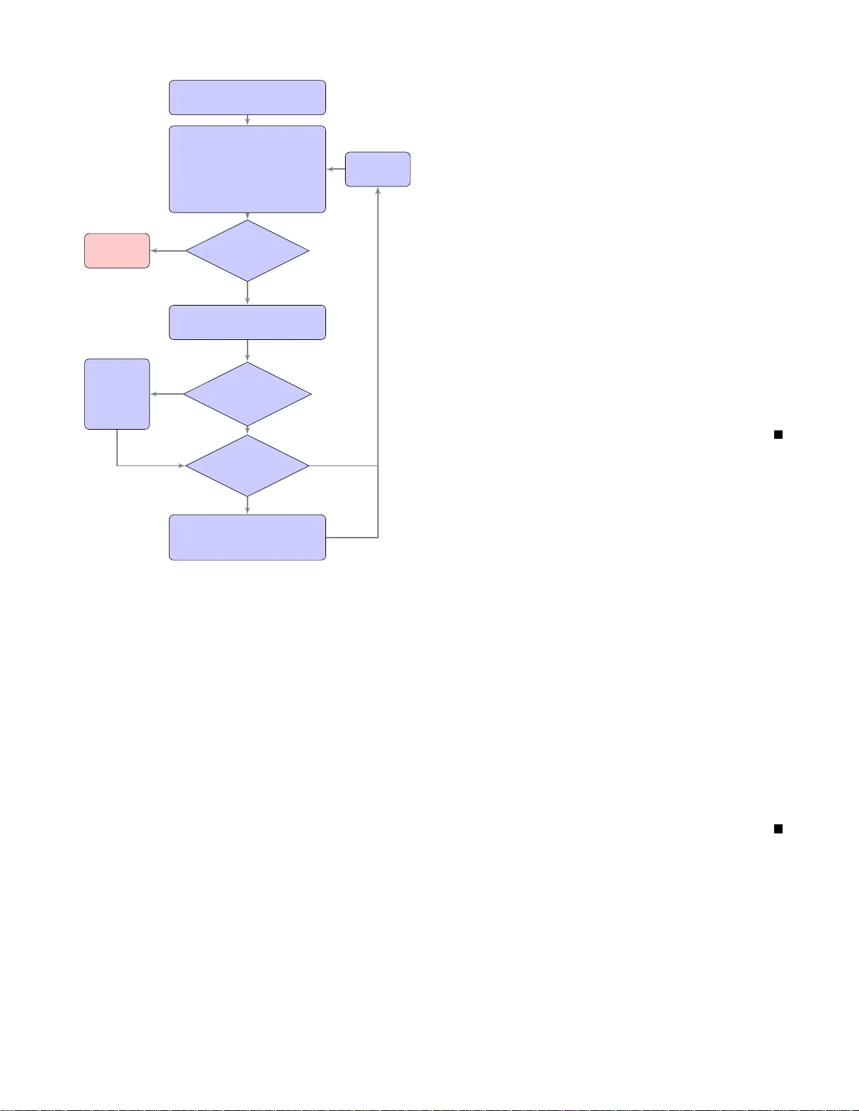
External Constraint Handling for Solv ing Optimal Control Problem s with Simultaneous Approaches and Inter ior Point Methods Y uanbo Nie and Eric C. Kerrigan Senior Member , IEEE ©2019 IEEE. Persona l use of this materi al is permitted. Permission from IEEE must be obtaine d for all other uses, in any current or future media, includi ng reprinti ng/repu blishing this mat erial for adv ertisin g or promotional purposes, cre ating ne w collect i ve works, for re sale or redist ribut ion to servers or lists, or reuse of any copyrighte d compone nt of this work in other works. Abstract — Inactiv e constraints do not contribute to the solu- tion of an optimal control p roblem, but i ncrease the problem size and burden the numerical computations. W e present a nov el strategy f or handling inactive constraints efficientl y by systematically remo ving the inacti ve and r edundant co nstraints. The method is designed to be used together with simultaneous approaches under a mesh refinement framew ork, with mild assumptions th at th e original problem has feasible solutions, and the i nitial solve of the problem is successful. The method is tailored fo r i n terior point-b ased solvers, which are known to be very sensi t iv e to the ch oice of initial points in terms of feasibility . In the example p roblem sh own, the proposed scheme achiev es more than a 40% reduction in computation time. Index T erms — constrained control, optimal cont rol, predic- tive contro l I . I N T RO D U C T I O N Optimal c ontrol h as been very po p ular fo r a wide range of app lications, tha nks to its ab ility to hand le various types of con straints systematically . When f ormulatin g the op timal control pro blem (OCP), it is comm o n pra ctice to impo se a large num ber o f con straints to en sure all m ission specifi- cations ar e fulfilled . Howe ver, for th e solution ob tained, it is often the c ase th at o nly a small subset of the impo sed inequality co nstraints will actually be ac tive. Fu r thermor e, ev en for the ones in this small subset, th e duratio n for which each constraint is active is generally much shorter than the time dimension of th e OCP . On e example would be for the design of flight con trol systems: althou gh all limits of th e flight envelope need to b e sp ecified in th e pr oblem formu latio n for safety r equireme nts, o nly in rar e (a bnorm al) situations is it the case that some limits will b e reach e d . In n u merical op tim al contr ol, the OCPs are transcr ibed into sparse no n linear p rogram ming (NLP) prob lems. A dis- tinction can b e m ade h ere b etween simultaneo us and seque n - tial app roaches, depend ing o n whethe r all or just th e co ntrol trajectories are d iscretized as d e cision variables [1 ]. For this work, we f ocus on the simultaneo us approa c h. The m ain co mputation al overheads f or solv ing the NLP problem s are directly related to the num ber of decision variables and co nstraints. Thus there exist significant com- putational b enefits to exclude inactiv e constraints in th e Y uanbo Nie and E ric C. Ke rrigan are with the Department of Aero- nautic s, Imperial Colle ge London, SW7 2AZ, U.K. yn 15@ic.ac.uk , e.kerrigan@im perial.ac.uk Eric C. Ker rigan is also with the Department of Electric al & Electronic Engineeri ng, Imperial College L ondon, London SW7 2AZ , U.K. Accept ed version to be published in: IEE E Control Systems L etters problem fo rmulation . One p ossibility is to only inclu de the constraints that are determ ined to be active. Based on this, an external strategy for the handling of path constraints with activ e-set based NLP solvers has b een pr oposed in [2]. The idea is to first solve the unco nstrained pr oblem and determine which constrain ts are likely to b e acti ve based on constraint violations. These constraints are then add e d in the OCP and the prob lem is r epetitively solved un til all original constraints are satisfied. Howe ver , a fu ndamen tal prob lem arises when implementin g the same idea on interior point method (IPM) based solvers, since g o od perfo rmance h in ges on the initial point to be feasible, or at least close to feasible [3 ] . Another option is to remove con straints that are inac- ti ve. Removal of constraints for mo del p redictive co ntrol (MPC) has been studied to accelerate compu ta tio ns for linear MPC [4], tub e-based robust lin ear MPC [ 5] and rece n tly nonlinear MPC [6], with compu tational benefits clearly demonstra te d . Howev er , all of th ese are b ased on a qu adratic regulation cost, mak ing their application specifically aimed at re c eding hor izon contr ol of regulatio n tasks. In this pape r, we intro duce an external con straint handlin g (ECH) strategy that is tailor e d to IPM-based NLP solvers for solving a variety of OCPs. Implemen ted together with mesh refinement (MR) schemes, co nstraints that do n ot c o ntribute to the solution a r e systematically removed in th e pro blem formu latio n. Sp ecial attention is p aid to ensu r e feasibility of the initial po int. As a result, significan t co mputation al sa vings can be achieved. Section II gives an introd uction to numerical op timal con trol with d irect collocation. This is fo llowed by a discu ssion of the prop osed ECH strategy in Section III. A flight con trol exam ple is presen ted in Section IV to demon stra te the co mputation al b enefits. I I . N U M E R I C A L O P T I M A L C O N T R O L Generally speaking, optimization-based contr ol re quires the solution of OCPs exp r essed in th e g eneral Bolza form : min x,u,p,t 0 ,t f Φ( x ( t 0 ) , t 0 , x ( t f ) , t f , p )+ Z t f t 0 L ( x ( t ) , u ( t ) , t, p ) dt (1a) subject to ˙ x ( t ) = f ( x ( t ) , u ( t ) , t, p ) , ∀ t ∈ [ t 0 , t f ] (1b) c ( x ( t ) , u ( t ) , t, p ) ≤ 0 , ∀ t ∈ [ t 0 , t f ] (1c) φ ( x ( t 0 ) , t 0 , x ( t f ) , t f , p ) = 0 , (1d) with x : R → R n is th e state trajectory of the system, u : R → R m is the con trol inpu t trajectory , p ∈ R s are static parameters, t 0 ∈ R an d t f ∈ R are the initial an d ter minal time. Φ is the Ma y er c o st fun ctional ( Φ : R n × R × R n × R × R s → R ), L is th e La g range co st fun ctional ( L : R n × R m × R × R s → R ), f is the dy n amic constraint ( f : R n × R m × R × R s → R n ), c is the p a th con straint ( c : R n × R m × R × R s → R n g ) and φ is the b ound ary cond ition ( φ : R n × R × R n × R × R s → R n q ). In p ractice, mo st optim al con trol pro blems for mulated as (1) n eed to b e solved with numerical sch emes. Comp a red to sequ ential m ethods, simultaneo us method s have some advantages with regards to co m putation a l effi ciency , as well as in the treatmen t of path co nstraints and unstable dynam - ics [1]. In this paper, we will demo nstrate o u r p r oposed E CH strategy with the simultaneo us app roach of dire c t co llocation. A. Dir ect collo cation metho ds Direct colloc ation method s can b e categorized into fixed- order h metho ds [7 ], and variable-ord er p / hp method s [8], [9]. Here, we only provid e a high lev el overview . For a mesh of size N := P K k =1 N ( k ) , the states can b e ap proxim ated as x ( k ) ( τ ) ≈ ¯ x ( k ) ( τ ) := N ( k ) X j =1 X ( k ) j B ( k ) j ( τ ) , within mesh in terval k ∈ { 1 , . . . , K } , wh ere N ( k ) denotes the number of collocation points for interval k and B ( k ) j ( · ) are basis fu nctions. For typica l h methods, τ ∈ R N takes values on the interval [0 , 1 ] rep resenting [ t 0 , t f ] , and B ( k ) j ( · ) a r e el- ementary B-splines of various order s. For p / hp method s, τ ∈ [ − 1 , 1] a nd B ( k ) j ( · ) are Lagr ange in terpolating poly nomials. W e use X ( k ) j and U ( k ) j to r epresent the app r oximated states and inpu ts at colloc a tio n p oints, e.g. X ( k ) j = ¯ x ( k ) ( τ ( k ) j ) ∈ R n , wher e τ ( k ) j is the j th collocation poin t in mesh inte r val k . Consequently , the OCP (1) c a n be app r oximated by min X,U,p,t 0 ,t f Φ( X (1) 1 , t 0 , X ( K ) f , t f , p ) + K X k =1 N ( k ) X i =1 w ( k ) i L ( X ( k ) i , U ( k ) i , τ ( k ) i , t 0 , t f , p ) (2a) for i = 1 , . . . , N ( k ) and k = 1 , . . . , K , subject to, N ( k ) X j =1 A ( k ) ij X ( k ) j + D ( k ) i f ( X ( k ) i , U ( k ) i , τ ( k ) i , t 0 , t f , p ) =0 (2b) c ( X ( k ) i , U ( k ) i , τ ( k ) i , t 0 , t f , p ) ≤ 0 ( 2 c) φ ( X (1) 1 , t 0 , X ( K ) f , t f , p ) =0 (2d) where w ( k ) j are the qu a drature weights for th e chosen dis- cretization, A ( k ) is the numerica l differentiatio n matrix with element ( i, j ) deno ted by A ( k ) ij and D ( k ) i is a row vector . The discretized pro blem can th en be solved w ith off-the- shelf NL P solvers. The N L P solver generates a discretized solution Z : = ( X , U , p, τ , t 0 , t f ) as sam pled data points. Interpo lating splines may b e used to constru ct an appro xima- tion o f th e con tinuou s- tim e optimal trajectory t 7→ ˜ z ( t ) : = ( ˜ x ( t ) , ˜ u ( t ) , t, p ) . The quality o f the inter p olated solution needs to be assure d through error analysis, assessing the lev el of accu racy and constraint satisfaction at a mu ch h ig her resolution than the discretization mesh. If n ecessary , app r opriate m odifications mu st be made to the discretizatio n m esh, until the solutio ns o btained with the new mesh fulfills all p redefined error to lerance levels (e.g . the absolu te loca l err or η tol and the abso lute local constra in t violation ε c tol ). Th is pro cess of MR is c r ucial in solvin g large-scale pro blems efficiently . For instance, it took 6 MR iterations fo r the example problem to be solved to a specific tolerance level. This level of a c c uracy was no t achievable with a ny un iform mesh using the same deskto p com p uter . I I I . E X T E R N A L C O N S T R A I N T H A N D L I N G A. Active and in a ctive con straints A constraint (1 c) is conside red a ctive if its presence influences the solu tion z ∗ ( · ) : = ( x ∗ ( · ) , u ∗ ( · ) , p ∗ , t ∗ 0 , t ∗ f ) . A constraint is inactive if it can b e re moved without affecting the solution. T o cla r ify , conside r a simplified prob lem: y ∗ ∈ arg min y Φ( y ) subject to c ( y ) ≤ 0 , where we nee d to identif y co n ditions such that co nstraints can be determine d to be active. The most obvious cr iter ia is wh en the solution y ∗ is at the b oundar y of c i ( y ) ≤ 0 , i.e. c i ( y ∗ ) = 0 . Additionally , co nsider the Lagr angian L := Φ( y ) + λ T c ( y ) and the necessary op timality co nditions (Karush-Kuhn -T u cker ( KKT) con ditions): ∂ Φ( y ) ∂ y | y = y ∗ + λ ∂ c ( y ) ∂ y | y = y ∗ = 0 , c ( y ∗ ) ≤ 0 , λ ≥ 0 , λ ◦ c ( y ∗ ) = 0 , with ◦ the Hadamard produc t. From the includ ed co m- plementary slackness conditio n , we know that for strictly positive Lagr ange mu ltipliers ( λ i > 0 ), th e co rrespon ding solution will have c i ( y ∗ ) = 0 , i.e. the constrain t is active. B. Iden tifying active co nstraints in o ptimal contr ol Theoretically , the above-mention ed analysis ap plies o nly to the con tinuou s OCP formulatio n (1). Add itional chal- lenges will arise in pra c tice when solv ing the discretized problem (2) num erically: the NLP solver will o nly return the values of the discretized state X , input U , and L a g range multipliers Λ at colloc a tion points. T o estimate th e constraint activ atio n status in- between collocation points, a criteria can b e introduce d based on the interpolated con tinuou s trajectory ˜ z . By d efinition, in e q uality constraints are activ e if the m a gnitude of the d ifferences between the ac tu al con straint c l ( ˜ z ( · )) an d the user-defined constraint boun ds are zero . Du e to nume r ical inac curacies, howe ver , ther e will always be a rema inder . Thus, we consid e r a constraint to be po tentially active if th is d ifference is smaller than the constrain t violation to lerance ǫ c tol . Note th at the word po tentially is used to e m phasise that, for n u merical schemes u nder limited machine pre c isio n , no concrete determ ination of co nstraint active status can be made. O n th e other hand , we k now th at o nly if the identified inactive constraints are tr u ly inactive, then ca n they be removed from the OCP withou t affecting the solution s. Thus, it would be much m ore pref erable to erron eously identify inactive co n straints as active, than the opposite situation . For this r eason, we also use the multip lier info rmation to enforce a larger (mo re conservativ e) selectio n of potentially activ e con stra ints. Here, a similar num erical challeng e arises: with limited machine precision , even when the corr espondin g constraints ar e inactiv e, th e m ultiplier values a r e ra rely truly equal to zero . T o id entify the regions where the con straints are likely to be a ctiv e, the n umerical multiplier data Λ is first norm alized between 0 a n d 1 for each con straint c l ( Z ) ≤ 0 . Signal processing algo rithms can be used to identify different in tervals wher e th e behaviour o f Lag r ange multipliers have significant c hanges, f or example using the M AT L A B findc hangepts fun ction. For each identified interv al T i , the mean value o f the normalized multipliers ( ¯ Λ T i ) is c alculated and co m pared based on the following criteria: if ¯ Λ T i ≥ ζ constraint po ten tially activ e in interval T i otherwise constraint po ten tially inactive in inter val T i with ζ a threshold p arameter . T o sum up, the following definition is u sed to de termine whether th e con straints ar e po te n tially a ctiv e or poten tially inactive at different collocation po ints. Definition 1: A co n straint c l ( X i , U i , τ i , t 0 , t f , p ) ≤ 0 is potentially active at tim e t i := t i ( τ i , t 0 , t f ) if o n e of the following criteria is met: • Between adjacen t collo cation points ( t ∈ [ t i − 1 , t i +1 ] ), c l ( ˜ x ( t ) , ˜ u ( t ) , t, p ) ≥ − ǫ c tol holds, with ǫ c tol > 0 . • ¯ Λ T i ≥ ζ , with t i ∈ T i . Otherwise, a con straint is potentially ina ctive at time t i . In add itio n to identifyin g the time instances a t which certain constraints may be p otentially inactive, it is also preferab le to determine the sets of constrain ts that nev er become active at all times. Definition 2: A co n straint c l ( X i , U i , τ i , t 0 , t f , p ) ≤ 0 is potentially r ed unda nt if for all t i := t i ( τ i , t 0 , t f ) with i = 1 , . . . , N , the constrain ts c l ( X i , U i , τ i , t 0 , t f , p ) ≤ 0 are poten tially inactive. Otherwise, this set of con straints is potentially enfo r ce d . C. Initia liza tio n for in terior point methods Interior point method s (IPMs) f or solving NLPs were introdu c ed in the early 1 960s [10]– [12] an d have b ecame very po pular in n u merical op timal control. The idea is to augmen t the o bjective function with barrier function s of constraints in o r der to enfor ce their satisfaction. Potential solutions will iterate o nly in the feasible region fo llowing th e so-called central path, resulting in a very efficient algorithm . Standard inter ior po int meth ods are sensitiv e to the choice of a starting point. T o ensure that the initial guess is strictly feasible with respect to con straints, various initialization methods h ave b een developed ( e.g. [1 3 ] an d th e collective study in [7 ]) and implemented in mod ern solvers. T o ensure reliable and efficient comp utation of the initial- ization alg o rithm, as well as the subsequen t NLP iteratio ns, se veral criteria [ 3] can be fo r mulated regarding ide a l initial points fo r IPMs. The ideal initial poin t should : • satisfy or be close to primal and dual f easibility , • be clo se to the central p ath, • be as close to optimality as possible. Because of these ch aracteristics, external constrain t han- dling schemes developed for active-set based SQP so lvers, such as [2 ], are no t suitable for IPM-based solvers. By first solving the unc o nstrained problem and gr a dually adding con- straints based on the constraint viola tio n erro r , the solution of previous solves will all b e infeasib le f or the new OCP formu latio n, and the solution may undergo d r astic chan ges as well. For I PM-based NLP solvers, this would lead to a higher com p utational overhead for initialization , a s well as higher chan ces f or the iteration s to freq uently enter the slow and u nreliable feasibility restoration p hase. D. Pr op osed S cheme for Constraint Han dling Based on th e criter ia presented in Section III -B and the characteristics of IPMs as discussed in Section III-C, a strategy for efficiently hand ling con straints in OCPs solved with IPM-based NLP solvers is p ropo sed , with the work -flow presented in Fig ure 1. Th e ap proach is called external , since the m odifications to th e OCP are made at the M R iteration lev el, instead of du ring the NLP iterations. The unm odified OCP is first solved o n the initial co a rse mesh. Even with all co nstraint equations in cluded, the com- putation time will still be quite low at this stag e due to th e small pro blem size. Once th e solution is ob tained, potentially inactive constrain ts and poten tially redu ndant con straint sets can be identified, ba sed on Definitions 1 and 2, with poten- tially redu ndant constraints d irectly excluded from th e OCP formu latio n. Fur thermor e, if the problem has a fixed termina l time, i.e. the time instance corresp onding to a m esh po int will not chan g e, then po tentially inactive constrain ts in the potentially enf orced con straint sets may also be removed. Recall that it is prefer a ble to erro neously iden tify an ina c - ti ve con straint as potentially active, rather tha n the opposite. It is th erefore often a go od idea in practice to enlarge the intervals with p otential constraint activ ation b y an inter val of length β in each direction , with β either fixed or a d apting during the MR pro cess. Th is adap tation also guaran tees the conv ergence of the overall scheme, i.e. in th e worst case, β can be sufficiently large to impose the constraints f or the whole traje c tory , with th e o riginal pro blem recovered. In-between M R iterations, spe cial atten tio n must be mad e to co nstraints and co nstraint sets that were determined to b e potentially inactive or re dunda n t in the previous solves. If they n ev er become a c ti ve or enforced again, the constrain t re- moval pr ocess may continue until MR is converged. But there will b e th e cha n ce, af ter refin ing the mesh, the con straint violation erro r analysis dictates that certain co n straints and Solve u nmodified OCP (coarse mesh) Error analysis and mesh refinement; identify potentially inactive constraints and potentially redund ant constraint sets based on the unm odified pr oblem all erro rs within tolerance? Remove potentially redu ndant constraint sets fro m OCP fixed terminal time p r oblem? Remove potentially inactive constraints from OCP any constraint reactiv ated? Solve the aux iliary f easibility problem and use the solution as initial gu e ss Solve the new OCP stop yes no yes no yes no Fig. 1. Overvi e w of the proposed extern al constraint handli ng scheme constraint sets tha t have been re m oved ear lier may becom e potentially active or en forced a g ain. If this h a p pens, they need to be inclu ded again to ensu re that th e solution of th e modified OCP is equiv alent to the un modified prob lem. Note tha t the p revious solutio n will no longe r be a feasible initial guess for the new problem form ulation. T o assist the subsequen t solve o f NLPs, the following auxiliary f easibility problem ( AFP) can be so lved befo r e proceed in g: J ∗ := min X,U,p,t 0 ,t f n g X l =1 s l (3a) subject to, fo r i = 1 , . . . , N ( k ) and k = 1 , . . . , K , ˜ N X j =1 A ( k ) ij X ( k ) j + D ( k ) i f ( X ( k ) i , U ( k ) i , τ ( k ) i , t 0 , t f , p ) =0 (3b) c ( X ( k ) i , U ( k ) i , τ ( k ) i , t 0 , t f , p ) ≤ s, with s ≥ 0 (3c) φ ( X (1) 1 , t 0 , X ( K ) K , t f , p ) =0 (3d) with s ∈ R n g slack variables. The initial gue ss for the AFP will be ˜ Z : = ( ˜ X , ˜ U, p, ˜ τ , t 0 , t f ) , the values of the interpolated solution ˜ z at the collo cation poin ts of the refin ed mesh. E. Pr o p erties of the external constraint hand ling strate gy It is possible to d erive p r oofs of fea sib ility and op timal- ity inv ariance for the removal of constraints on a given discretization mesh. Ho wev er , with the size of the mesh changin g throu ghou t the refinement process, the analy sis of erro rs, and ide n tification of constraint activ ation status (Section II I-B) are all subjec t to consid erable uncer tainties. When a co n straint or con straint set must b e in cluded a gain in the prob lem, it will be ch allenging to ensure that the subsequen t OCP solve can b e supplied with a feasible initial guess. Th e intro duction of the AFP is the answer to this challenge, with its solutio n guar anteed to b e a f easible poin t for th e corre sp onding original OCP . Pr opo sition 1: If the origin al OCP (2) h as feasible poin ts, then a solution to the aux iliary feasibility pro blem (3) will be a feasible p oint of (2) on the same d iscr e tization mesh, and (3) will have correspond ing ob jectiv e value J ∗ = 0 . Pr oof: If Z : = ( X , U, τ , t 0 , t f , p ) is a feasib le p oint of ( 2), then ( 2c) must hold. With s ≥ 0 , th e solutio n for the AFP (3) will be the situation where P s l = 0 , and (2 c) guaran tee s the existence of such a solution. Now , fo r th e very sam e rea so n, we need to obtain a suitable initial g uess for the slack variables s in the AFP . One possible way is by calcu lating the co nstraint vio lation errors o f the interpolated solutions o n the refined m esh. Pr opo sition 2: Define ˜ s ∈ R N × n g as th e absolute local constraint violation er ror ǫ c ( t ) calculated at th e collocation points of the r e fined mesh, with the u pdated initial g uess ˜ Z : = ( ˜ X , ˜ U, p, ˜ τ , t 0 , t f ) . For any set { ¯ s ∈ R n g | ¯ s l ≥ max i =1 ,...,N ( ˜ s i,l ) , l = 1 , . . . , n g } im plemented as the initial guess f or s , the AFP (3) will have a strictly feasible in itial point with respect to th e co nstraints (3 c). Pr oof: ˜ s i,l := | min( − c l ( ˜ X i , ˜ U i , p , ˜ τ i , t 0 , t f ) , 0) | by definition, fo r all i = 1 , . . . , N and l = 1 , . . . , n g , • if c l ( ˜ X i , ˜ U i , p , ˜ τ i , t 0 , t f ) < 0 , i.e. the constraint is satisfied and the solution is not on the bound ary , then ˜ s i,l = 0 , thu s c l ( X i , U i , τ i , t 0 , t f , p ) < ˜ s i,l holds. • if c l ( ˜ X i , ˜ U i , p , ˜ τ i , t 0 , t f ) = 0 (constraint satisfied and solutio n is on the bou ndary ) or c l ( ˜ X i , ˜ U i , p , ˜ τ i , t 0 , t f ) > 0 (con straint violation occu rs), then c l ( X i , U i , τ i , t 0 , t f , p ) = ˜ s i,l holds. Therefo re, c l ( X i , U i , τ i , t 0 , t f , p ) ≤ ˜ s i,l will always be true. From ¯ s l ≥ max i =1 ,...,N ( ˜ s i,l ) , it can be con cluded th at c l ( X i , U i , τ i , t 0 , t f , p ) ≤ ¯ s l holds. W e can now sh ow that, except for the initial so lve, all subsequen t solves will h av e feasible in itial g uesses. Pr opo sition 3: If the unmo dified O CP has f easible points, and the initial solve of the discretized OCP has been succe ss- ful, the n all sub sequent solves of OCPs and AFPs with m esh refinement schemes and the pr oposed external co nstraint handling method w ill have a feasible initial po int with respect to th e constra in ts (2c) or (3 c). Pr oof: For any interpolated solution ˜ Z : = ( ˜ X , ˜ U, p, ˜ τ , t 0 , t f ) on the new mesh, if ( 2c) is no t satisfied, then th e correspo n ding AFP will b e solved and Propo sition 2 ensures th at AFP will have a feasible initial guess. From Proposition 1 the so lution of the AFP will be a fea sib le initial guess for the subsequ ent OCP solve. F . A practically more efficient alternative imp lementation The pro posed external constraint han dling scheme can guaran tee feasible initial points under con ditions stated in Proposition 3 . Ne vertheless, it is not efficient in prac tice . The f requen t solve of AFPs ar e not only time consu m ing, but are o f ten no t necessary . Recall the c o nditions regard ing ideal initial guesses for IPM meth ods. It is no t nece ssary to satisfy prima l a nd dual feasibility — rather, one only need s to be close to fulfillment. In p ractice, the computational p erform ance of a moder n IPM that u ses n ear-feasible in itial guesses is very much compar able to using feasible initial points. In addition, constraint satisfaction for simple bou nds can be computatio nally m u ch easier to achieve by the NLP solver , thus th ere is no need to enf orce tho se thr ough the solve of an AFP . Thus, a practically more e fficient version of the exter- nal ha n dling scheme can be formu lated, by r estricting the condition s for solving the AFP to the M R iteration w h en a po te n tially redu ndant path constra int set turns into a potentially enf orced path constrain t set. I V . E X A M P L E T o demo nstrate the com p utational benefits of the prop osed ECH schem e, we show an p roblem that is relatively large in the horizon len gth. T he task inv olves finding a fuel-op timal flight path o f a comme rcial aircraft wh ere authorities have identified five non- flig ht zones ( NFZ) fo r the aircraft to av oid. From sim p le fligh t mechan ics with a flat earth assumption, both the long itudinal and lateral mo tion of the aircraf t can be describ ed by the d ynamic equ ations ˙ h ( t ) = v T ( t ) sin( γ ( t )) ˙ P OS N ( t ) = v T ( t ) cos( γ ( t )) co s( χ ( t )) ˙ P OS E ( t ) = v T ( t ) cos( γ ( t )) sin ( χ ( t )) ˙ v T ( t ) = 1 m ( t ) ( T ( v C ( t ) , h ( t ) , Γ( t )) − D ( v T ( t ) , h ( t ) , α ( t )) − m ( t ) g sin( γ ( t ))) ˙ γ ( t ) = 1 m ( t ) v T ( t ) ( L ( v T ( t ) , h ( t ) , α ( t )) cos( φ ( t )) − m ( t ) g cos( γ ( t ))) ˙ χ ( t ) = L ( v T ( t ) , h ( t ) , α ( t )) sin ( φ ( t )) cos( γ ( t )) m ( t ) v T ( t ) ˙ m ( t ) = F F ( h ( t ) , v C ( t ) , Γ( t )) with h the a ltitu de [m ], P OS N and P OS E the no rth and east p osition [ m], v T the true airspeed [m/s], γ the flight path ang le [rad ] , χ the tracking ang le [rad] , an d m the m ass [kg]. T , L , D are the thrust, lift an d drag for ces. F F is the fuel flow mo d el, requiring an input o f calibr ated airspeed v C , which can be related to v T via a conversion. 0 2 4 6 8 10 10 5 0 2 4 6 8 10 5 ORG DES 5 2 1 3 4 Fig. 2. The fuel-optimal flight profile for the exampl e problem Additionally , g = 9 . 8 1 m/s 2 is g ravitational acceleration. W e have three control inp u ts, the roll ang le φ in [r ad], the throttle settings Γ nor m alized between 0 and 1, an d the angle of attac k α in [rad] . Further details of the mod elling of a Fokker 50 aircraf t can b e o btained fr o m [14]. The av o idance of NFZs can be implemen ted with the following path con straints ( P OS N ( t ) − P OS N N ) 2 + ( P OS E ( t ) − P OS E N ) 2 ≥ r 2 N with P OS N N and P OS E N the no r th an d east position of the center o f the non -flight zones, an d r N the radius. The prob lem will have the bo undar y c ost Φ( x ( t 0 ) , t 0 , x ( t f ) , t f , p ) = − m ( t f ) ( maximize th e mass at the end o f the flight, with fixed t f = 74 7 5 s), sub ject to th e dynamics and path con straints. Furthermo re, variable simple bound s are imposed togeth er with th e bou ndary cond itions. The OCP is transcrib ed usin g the op timal control software ICLOCS2 [15] with He rmite-Simpson discretization , and solved with I PM-based NLP so lver IPOPT [16] ( versio n 3.12.4 ). All co mputation results shown were o b tained on an Intel Cor e i7-477 0 comp uter with 16 G of RAM. Figure 2 illustrates th e results solved to a user-defined to le r ance. Using th e prop osed external c onstraint h a ndling scheme, we first solved the prob lem with a worst-case buffer interval setting of β = 0 s. The history for co nstraint activ ation inter- vals imp lemented in the OCP are demon strated in T able I. It can be seen that in the initial solve (MR iter ation 1), all constraint sets are e n forced an d all constrain ts a re tr e ated as potentially active. Based only on the solution from th is coarse grid, the ECH meth od co rrectly identified that the constraint sets related to NFZ 2, 3 and 5 are all p otentially redund ant. It also determined that constraints related to NFZ 1 are o nly potentially acti ve near the end of the flight, whereas f o r NFZ 4 they are at the b eginning of the mission . In later iterations o f the M R, these intervals had only some minor ad justments. It can be seen tha t without imp lement- ing any buffer interval, we d o see occasions where active constraints got err oneou sly identified as ina c ti ve fo r finer meshes. Howe ver , the co nstraint violation erro r analysis in the MR process cor rectly id entified these situations and made correction s according ly . T ABL E I E X T E R N A L C O N S T R A I N T H A N D L I N G H I S T O R Y : A I R C R A F T F L I G H T P RO FI L E ( t 0 = 0 S , t f = 7475 S , β = 0 S ) Constraint Activ ati on Intervals Implemented in the OCP [ s ] MR Iteration 1 MR Iteration 2 MR Iteration 3 MR Iteration 4 MR Iteration 5 MR Iteration 6 (K = 40) (K = 81) (K = 136) (K = 176) (K = 207) (K = 256) NFZ 1 [ t 0 , t f ] [6900 7092] [6996 7114] [7056 7162] [7071 7140] [7074 7150] NFZ 2/3/5 [ t 0 , t f ] ∅ ∅ ∅ ∅ ∅ NFZ 4 [ t 0 , t f ] [671 863] [743 942] [767 875] [77 4 880] [774 878] T ABL E II C O M P U TATI O N A L P E R F O R M A N C E C O M PA R I S O N Standard W ith ECH With ECH Solve ( β = 0 s) ( β = 747 . 5 s) T otal Comp. 130.54 92.14 78.27 Time [s] (29% lower) (40% lower) MR Iterations 6 6 6 Re-comp. 21.82 13.50 10.78 Time [s] (38% lower) (50% lower) Fuel Used [kg] 1787.6 1787.6 17 87.6 T able II compar es the comp utational perf o rmance of the standard solve, as well a s solves with e xternal constrain t handling using the alter native ECH implementatio n (allowing near-feasible in itial gu esses) described in Section III- F, with two different buffer in ter val settings. W ith the worst-case setting of β = 0 , th e total comp u tation time saw a 29% reduction , while the n umber of MR iterations r e mained the same. Choosing a much more co nservati ve buffer interval setting of β = 0 . 1( t f − t 0 ) = 747 . 5 s further imp roved this time reductio n to 4 0%, d ue to the fact that initial g u esses were feasible fo r all later MR iterations. For real-time applicatio ns, it is useful to consider the re- computatio n time fo r solv ing the OCP proble m ag ain with the fina l (refined) discre tization mesh, using the obtained solutions as in itial gu e sses. For the ECH meth od with β = 747 . 5 s, th e time taken w as o nly half compa r ed to the standard solve. Th e refore, the b e n efits of the propo sed scheme can b e seen for b oth off-line an d online app lications. V . C O N C L U S I O N S A strategy h a s been developed to system atically identify and hand le inactive constraints and red undan t co nstraint sets for numerically solvin g op timal con trol p roblems togethe r with mesh refinem ent sche m es. Unlike pr evious work tha t would always result in infeasible initial guesses for inter- mediate steps, th e pro posed scheme is capable of p rovid- ing g uarantees on th e feasibility of in itial poin ts in mesh refinement iterations. Th e method only re quires some mild condition s — the origin al OCP to h ave feasib le po ints, and the initial solve of the discre tized OCP to be su c cessful, making it particu larly suitable f or OCP toolbo xes that utilize IPM-based NLP solvers in lowering the computatio nal cost. Due to limitatio ns in time an d space, we o n ly illustrated the pr oposed extern al constraint h andling m ethod with di- rect collocatio n. W e note that similar benefits should be obtainable , af ter som e ad aptations, with o ther simultaneou s methods, su ch as direct multiple shooting. This m ig ht also be possible for sequential m ethods, such as d irect single shooting. Moreover , it would b e inte r esting to test a slightly altered version o f our pro posed co n straint r emoval meth o d with activ e-set based NLP solvers — this could be com pared under a mesh refinemen t sch eme against ear lier work [2 ], which explo its constraint add ition instead. R E F E R E N C E S [1] L. T . Biegle r , “ An overvi e w of simultaneo us strategie s for dynamic optimiza tion, ” Chemical Engineering and Proc essing: Process Inten- sificati on , vol. 46, no. 11, pp. 1043–1053, 2007. [2] H. Chung, E. Polak, and S. Sastry , “ An externa l acti ve-set strategy for solving optimal contro l problems, ” IEEE T ransactions on Automatic Contr ol , vol. 54, no. 5, pp. 1129–1133, 2009. [3] J. Gondzio, “Crash start of interior point methods, ” E ur opean Journal of Operation al Researc h , vol. 255, no. 1, pp. 308–314, 2016. [4] M. Jost, G. Pannocchia , and M. M ¨ onnigmann, “Constraint remov al in linear mpc: An improv ed criterion and complexi ty analysis, ” in Eur opean Contr ol Confer ence (ECC) , pp. 752–757, IEEE, 2016. [5] M. Jost, G. Pannocch ia, and M. M ¨ onnigmann, “ Accele rating tube- based model predicti ve control by constrai nt remov al., ” in 54th IEEE Confer ence on Decision and Contr ol (CDC) , pp. 3651–3656, 2015. [6] R. Dyrska, , and M. M ¨ onnigmann, “ Accelerat ing nonlinear model pre- dicti ve control by constraint remov al, ” in Proc. 6th IF AC Confer ence on Nonlinear Model Predi ctive Contr ol , 2018. [7] J. T . Betts, Practical Methods for Optimal Contr ol and Estimation Using Nonline ar Pro gramming : Second Edition . Advance s in Design and Control, Society for Industrial and Applied Mathemat ics, 2010. [8] F . Fahro o and I. M. Ross, “ Adv ances in pseudospectral methods for optimal control, ” in A IAA guidance , navigation and contr ol confer ence and exhibi t , p. 7309, 2008. [9] F . L iu, W . W . Hager , and A. V . Rao, “ An hp mesh refinement method for optimal control using discontinuity detecti on and mesh size reducti on, ” in 53th IEE E Confer ence on Decision and Contr ol (CDC) , pp. 5868–5873, IEEE, 2014. [10] A. V . Fiacco and G. P . McCormick, “Programming under nonlinea r constrai nts by unconstrained minimizati on: a primal-dua l method, ” tech. rep., Research Analysis Corp Mclean V A , 1963. [11] A. V . Fiacco and G. P . McCormick, “The sequenti al unconstra ined minimizat ion technique for nonline ar programing, a primal-dual method, ” Manageme nt Science , vol. 10, no. 2, pp. 360–366, 1964. [12] A. V . Fiacco and G. P . McCormic k, “Extensions of SUMT for nonlin- ear programming: equality constraints and extrapola tion, ” Manag ement Scienc e , vol. 12, no. 11, pp. 816–828, 1966. [13] S. Mehrotra , “On the implementat ion of a primal-dual interior point method, ” SIAM J ournal on optimization , vol. 2, no. 4, pp. 575–601, 1992. [14] Delft Unive rsity of T echnology , P erformance Model F okker 50 , 2010. [15] Y . Nie, O. J. Faqir , and E. C. Ker rigan, “ICLOCS2: Solve your optimal control problems with less pain, ” in Pro c. 6th IF AC Confer ence on Nonline ar Model Pred ictiv e Contr ol , 2018. [16] A. W ¨ achter and L. T . Biegle r , “On the implementati on of an interi or- point filter line-search algorithm for large -scale nonlinea r program- ming, ” Mathemat ical pro gramming , vol. 106, no. 1, pp. 25–57, 2006.