A Data Driven Vector Field Oscillator with Arbitrary Limit Cycle Shape

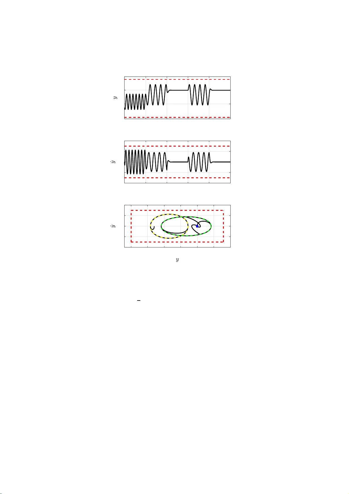
A Data Driv en V ector Field Oscill ator with Arbitrary Limit Cycle Sh ap e V en us P asandi a,b , Aik o Dinale b , Mehdi Keshmiri a , Daniele Pucci b ∗ † Octob er 11, 2019 Abstract Cyclic motions in v ertebrates, including heart b eating, breathing and w alking, are deriv ed by a netw ork of biological oscillators having fascinat- ing features suc h as entrai nment, enviro nment adaptation and robustness. These features encouraged engineers to use oscillators for generating cyclic motions. T o this end, it is crucial to hav e oscillators capable of character- izing any p erio dic signal via a stable limit cycle. In this p ap er, w e prop ose a 2-dimensional oscillator whose limit cy cle can be matched to any p eri- odic signal depicting a non-self-interse cting curv e in the state space. In particular, the prop osed oscillato r is designed as an autonomous vector field d irected tow ard the desired limit cycle. T o this purp ose, t h e desired reference signal is parameterized with resp ect to a state-dep end ent phase v ariable, then t he oscillator’s states track the p arameterized signal. W e also presen t a state transformatio n t ec hnique to bound th e oscill ator’s out- put and its first time deriv ativ e. The soundn ess of the prop osed oscillator has been verified by carrying out a few simulations. 1 INTR O DUCT IO N Nonlinear oscillato rs ha ve b een widely used by the eng ineering communit y to mo del and co nt rol physical phenomena [1 –3]. Their in teresting features such a s ent rainment, synchronization and smo oth mo dulation of the o utput signal make them appropria te for rob otics applications such as cyclic motions of manipula- tors or legged rob ot lo co motion. Using oscillators for generating the reference tra jectory or control sig nal provides capabilities of smo othness, contin uit y , dis- turbance rejection and adaptation. The oscilla to r enco des the desire d refer ence tra jectory or control sig na l v ia a stable limit cycle. The essence o f well-known oscillator s, like the Matsuo k a’s a nd Hopf ’s, is their capability of generating limit cycles with a sp ecific shap e. Ho wev er, a specific limit cycle shap e constra in ts the types of signals that can b e generated. In this pap er, w e pro po se a tw o dimensional oscillato r which can genera te any perio dic tr a jector y , depicting a non-self-intersecting curve in the sta te spa ce. ∗ a Isfahan Universit y of T echno logy , Isfahan, Iran, venus.pa sandi@me.i ut.ac.ir, mahdi k@cc.iut.a c.ir † b Istituto Italiano di T ecnologia, Genoa, Italy , aiko.din ale@iit.it , daniel e.pucci@i it.it Assuming the desired limit cycle is defined b y a Ly apuno v function, the problem of designing a dynamical system with a desir ed limit cyc le is express e d as the problem of c o nstructing a dynamical system for a desir ed Ly apunov function [4, 5]. Besides co nt rolling the limit cycle, such fr amework has b een ex- tended to non-a uto nomous dynamical systems to des ign transient tr a jectories and achiev e the des ired conv ergence [6 ]. Although these algorithms are in ter- esting from the mathematics p o int of view, they can not b e dire ctly applied for engineering purp oses b ecaus e o f their lack of ana lytical predictability . In fact, these alg orithms genera te different dyna mic str uctures for differe nt desir ed limit cycles and the pr op erties of the dynamics, like domain of attractio n and attracting rate, ar e not deter mined a priori. A widespread s tr ategy for designing a dynamica l system generating an ar- bitrary p er io dic s ignal is to transform a well-understo o d dynamical system into an o scillating o ne with desired limit cycle. F or instance, a linear spring- damp er system can g e ne r ate a v a riety of cy clic signals with the help of a forcing term. T o desig n an autonomous sy s tem, the forcing term is defined by a nonlinear function of a phase v ar iable and learned by standard machine learning tech- niques [7]. F rom a more genera l p ersp ective, the limit cy c le o f a phase oscillato r is mapp ed to the des ired p erio dic tra jectory in the sta te space throug h a pha se- depe ndent scaling function. Thus, a genera l family of nonlinea r pha se o scillators which can track almost any contin uous tra jectory is co ns tructed [8 ]. The phase of the dyna mical systems pro po sed in [7] and [8] is g enerated by an indepen- dent phase dynamics which re s ults in tra jectory tra cking and not limit cycle tracking. F ur thermore, the desired tra jectory is asymptotically s table and not asymptotically or bitally stable. T o provide limit cycle tracking of a desired p e- rio dic tra jectory , a Hopf ’s oscillator is altered b y tw o nonlinear functions which are deter mined such that the Poincar´ e-Bendixson theorem is satisfied in a pre- defined neig hbo rho o d of the limit cycle [9 ]. The framework guar a ntees lo cal stability and it is not straightforw ard to extend it for a chieving global stabilit y , since the Poincar´ e-Bendixso n theorem is no lo nger applicable. Another metho d for designing an oscilla tor is to use a data driven vector field whic h has b een originally pr op osed for genera ting a discrete system with an ar bitrary limit cyc le [10]. The discre te vector field genera ted in the neig hbor- ho o d of the limit cycle is appr oximated by a function, like a p olynomia l one, and hence, a contin uous dynamica l system with a lo cally stable desir ed limit cycle is created [1 1]. How ev er, to the b est of the author s’ knowledge, the poss ibilit y of designing a contin uo us no nlinear vector field for ensuring the globa l sta bilit y of the desired limit cycle has no t b een explored yet. In the present pap er, we prop ose a t w o dimensional contin uous dynamical system that can track any non- self-intersecting close d tra jectory in the state space. The main idea is to g enerate a data dr iven vector field directed to w ard the desir ed tra jectory . T o this purp ose, the desir ed tra jectory is parameterize d with resp ect to a state- de p endent phase v ariable. Then, the os cillator dynamics is des ig ned to track the pa rameterized tra jectory . Moreover, we pr op ose a state transformatio n metho d for genera ting a b o unded output by using the prop osed oscillator . The cont ribution of this pap er is threefold. Firs t, the prop os ed system pr ovides asymptotic orbital stability of the desired tra jectory . Second, the co n vergence to the desir ed tr a jector y is ir resp ective of the parameters of the system. Third, the prop osed o scillator is capa ble of g enerating bo unded o utput. The rest of the paper is or ganized as follows. Section 2 int ro duces the no - tations and definitions used in the pap er. It also r ecalls the concepts of o rbital stability a nd transverse dyna mics which will b e use d to prov e the asymptotic orbital stability of the desired tra jectory in the proposed oscillato r . Section 3 presents the mo del developmen t of the pro po sed oscillator . In Section 4, we mo dify the pr op osed o scillator to b ound the output and its firs t time deriv ativ e. Section 5 rep or ts simulation results. Finally , Section 6 concludes the pa p er with a few remarks a nd p ersp ectives. 2 BA CK GR OUND 2.1 Notations and Definitions • R and R + are the set of rea l and p os itive r eal num ber s . • The i th comp onent o f a vector q ∈ R m is wr itten a s q i . • Given a function g ( x ( t )) : R → R where t repr esents the time, its first deriv a- tives with resp ect to x and t are denoted a s g ′ = dg dx and ˙ g = dg dt , re sp e ctively . • A C k -function is a function with k co nt inuous deriv atives. • A function f ( t ) : [0 , ∞ ) → R is a T -p erio dic function if for some positive constant p , w e hav e f ( t + p ) = f ( t ) and T is the smalles t p with such prop erty . • A simple close d curve is a contin uous clos ed curve that do es not cr o ss itself. In mathema tica l word, γ : [ a, b ] → R n is a simple closed cur ve if γ ( a ) = γ ( b ) and additionally γ ( c ) 6 = γ ( d ), ∀ c, d ∈ [ a, b ). H ence, the simple closed curve γ is a one-to-one mapping from [ a, b ) to R n . 2.2 Stabilit y of a p eriodic tra jectory Given the dyna mical system ˙ x = f ( x ), where x ∈ R n is the state vector, the per io dic tra jectory x ∗ ( t ) is • stable if ∀ ǫ > 0 , ∃ δ > 0 such tha t k x ( t 0 ) − x ∗ ( t 0 ) k < δ ⇒ k x ( t ) − x ∗ ( t ) k < ǫ , • asymptotic al ly st able (AS) if it is stable and ∃ η > 0 that k x ( t 0 ) − x ∗ ( t 0 ) k < η ⇒ lim t →∞ x ( t ) = x ∗ ( t ) , • orbital ly stable (OS) if ∀ ǫ > 0 , ∃ δ > 0 such that inf ϕ k x ( t 0 ) − x ∗ ( ϕ ) k < δ ⇒ inf ϕ k x ( t ) − x ∗ ( ϕ ) k < ǫ, • asymptotic al ly orbital ly stable (A OS), called a ls o stable limit cycle, if it is orbitally stable and ∃ η > 0 that inf ϕ k x ( t 0 ) − x ∗ ( ϕ ) k < η ⇒ lim t →∞ inf ϕ k x ( t ) − x ∗ ( ϕ ) k = 0 . The a b ove stability definitions are stated from [12]. It is noteworthy that to verify either the OS or the AOS, we co nsider the time evolution of the distance betw een the sy stem’s states and the clo s ed set of the tra jectory x ∗ . On the other hand, to pr ov e the sta bility or the AS, we exa mine the time evolution of the distance be tw een the system’s s tates and a sp ecific p oint of x ∗ which changes w ith resp ect to time. Therefore, the stable/ AS conditions are stricter than O S/AOS. 2.3 T ransv erse Dynamics The OS pro p erty of a p erio dic tra jectory is usually in vestigated through t wo techn iques. In the fir st technique, the stability of a p e rio dic tra jectory o f a contin uous system is attributed to the sta bilit y of the equilibrium p oint of the corres p o nding discr ete map, called Poincar´ e ma p. A Poincar´ e map, known also a s fi rst r et urn map , is the intersection of the system’s tra jectory in the state space with a Poincar´ e section, that is a low er-dimensional h ype r surface transversal to the tra jectory under study . Usually , it is not p ossible to find the P oincar´ e map analytically . Therefor e , a linearization of the Poincar ´ e ma p is often computed numerically , and its eigenv a lues are used to v erify lo cal OS. In the second technique, the limit cycle is considered as a cla ss of inv aria nt sets a nd its stabilit y is in v estigated throug h the LaSalle’s inv ar iance principle. F or this pur po se, one uses a Lyapunov function that equals to zero along the tra jectory and is strictly po sitive elsewher e . An a pproach for constructing suc h Lyapuno v function is the tr ansverse dynamics , commonly called also moving Poinc ar´ e se ctions . In this approa ch, a tra nsversal hyper surface is defined in the state space which mov es along the tra jectory under study . Considering an n -dimensio na l T -p erio dic tra jector y x ∗ , a hypersurfa ce σ ( ϕ ) is defined for ϕ ∈ [0 , T ] where σ ( ϕ ) is tr ansversal to x ∗ ( ϕ ), i . e . ˙ x ∗ ( ϕ ) / ∈ σ ( ϕ ) and σ (0) = σ ( T ). Then, a new co or dinate system ( e , φ ) is established where the scalar φ represents which of the transversal surfaces σ is inhibited by the current state x , a nd the tr ansverse c o or dinate e ∈ R n − 1 determines t he lo c ation of x within the hypersurfac e σ ( φ ), with e = 0 implying that x = x ∗ ( φ ). The dynamics of the tra nsverse co ordina te is the transverse dyna mics. The sta bilit y of the e quilibrium po int e = 0 of the transverse dynamics ensures the OS o f the tra jectory x ∗ . In this way , one can analyze the stability analytically a nd characterize the stability r egion. F or more info r mation, th e reader can refer to [13–15]. 3 D A T A DRIV EN VECTOR FIELD OSCILLA- TOR In this section, w e desig n a contin uous 2-dimensional dynamical system tha t provides asymptotic orbital s tability of an y desired T -p erio dic function f ( t ) : [0 , ∞ ) → R de pic ting a simple clos e d cur ve in the state s pace. F rom her eafter, we co nsider one perio d of f ( t ), i . e . we ass ume the T -p erio dic function f ( t ) as f ( t ) : [0 , T ) → R . Consider the 2-dimensio nal dyna mical system des crib ed b y the following Figure 1: Geometrical representation of the target p oint. F o r every sta te of the system (squar e s ), there is a corr esp onding target p oint (circles) on the desired tra jectory (black curve). differential e quation ¨ s = f ′′ ( ϕ ) − α ( ˙ s − f ′ ( ϕ )) − β ( s − f ( ϕ )) , (1) where s = ( s, ˙ s ) ∈ R 2 represent the states, α, β ∈ R + are coefficients a nd ϕ is the phas e v ar iable defined based on s a s ϕ ( s ) =        f − 1 ( f l ) s ≤ f l { ϕ | f ( ϕ ) = s, f ′ ( ϕ ) ˙ s ≥ 0 } f l ≤ s ≤ f u , ˙ s 6 = 0 { ϕ | f ( ϕ ) = s, f ′ ( ϕ ) ≥ 0 } f l ≤ s ≤ f u , ˙ s = 0 f − 1 ( f u ) s ≥ f u , (2) where f l and f u are the low er and upp er b ounds of f . Conceptually , the prop osed dy namics (1) follows the tra jectory of the tar get p oint , i . e . a p oint defined on the function f in the state space with co ordinates ( f ( ϕ ( s )) , f ′ ( ϕ ( s ))). So, the ta r get p o int is asso c ia ted with the sta tes and rep- resents a parametr ization of the function f with resp ect to ϕ . Fig. 1 shows the relation b etw een the states and the co rresp onding targe t p oints. The black curve is the function f . Squar e s r epresent states at different time instants while circles are the corresp onding targe t p oints. Based on the pha s e v aria ble defi- nition (2), the state space is divided into three r egions. F or all the states in Region 1 ( R 1 ), the target p oint is the red circle with co ordinates ( f l , 0), while for all the states in Region 3 ( R 3 ), the target po int is the orang e circle with co ordinates ( f u , 0). F or the states in Reg ion 2 ( R 2 ), the target po int is a p o int on the function f with the sa me s co o rdinate as the state of the system. W e call the dynamics (1) alo ng with the phase defined in (2) as D ata driven V e ctor field Oscil lator (DV O). The r emainder o f this s e c tion is devoted to inv estigating the prop erties of the D V O. R emark 1. As the function f ( t ) is a simple clos ed curve in the state space, the target p oint assigned to s is unique. In light of the ab ov e, we assume from now o n that Assumption 1. f ( t ) is a T -p erio dic C 3 -function a s f ( t ) : [0 , T ) ⊆ R → R , (3) describing a simple closed o rbit in the plane ( f , ˙ f ). R emark 2. In addition to the limit cycle tracking, o ne can use D VO for p oint tracking where the tra jectory f is cons tant. In the case of po in t trac king, the dynamics (1) is simplified to the well-known P D control as ¨ s = − α ˙ s − β ( s − f ) . (4) The or em. Giv en that Assumption 1 is satisfied, and α is a p ositive fun ction and β is a p ositive constant then the tra jectory f ( t ) is the s e mi- stable limit cycle of the D V O expr essed in (1)-(2). The reg ion of a ttraction of f is D o = { ( s, ˙ s ) | ˙ s 2 ≥ f ′ 2 ( ϕ ) } . (5) The theorem states that a tra jectory conv erges to f if it is initialize d outside the clo s ed curve of f in the state space. Pro of: Let us define a weigh ted err o r e as e = 1 2 ( ˙ s 2 − f ′ 2 ) + β 2 ( s − f ) 2 − f ′′ ( s − f ) . (6) If ( s, ˙ s ) = ( f , f ′ ), then we have e = 0. T o show a lso that if e = 0 then ( s, ˙ s ) = ( f , f ′ ), let us sp ecify e in the three regions R 1 , R 2 and R 3 , defined based on the phase definition (2). In the case s ∈ R 2 , phase definition (2) results in s = f and the weigh ted error is simplified as e = 1 2  ˙ s 2 − f ′ 2  . (7) Thu s, ˙ s = f ′ if e = 0 . In the case s ∈ R 1 , w e have s < f l , f = f l , f ′ = 0 and f ′′ > 0. Thus, e is simplified as e = 1 2 ˙ s 2 + β 2 ( s − f ) 2 − f ′′ ( s − f ) , (8) which is the sum o f three p ositive terms. Thus ( s, ˙ s ) = ( f , f ′ ) if e = 0. The same res ults ar e true a ls o if s ∈ R 3 , but in this case s > f u , f = f u , f ′ = 0 and f ′′ < 0. Consequently , e = 0 iff the states s coincide the tra jectory of f in the state space, i.e. ( s, ˙ s ) = ( f , f ′ ). Thus, we co nsider v = 1 2 e 2 as the candidate Ly apunov function for proving the semi-stability of the limit cycle f . T o compute the time deriv ativ e of v , one needs to compute the time deriv ativ e of the phase v a riable ϕ on which the tra jectory f depe nds . Ba sed o n the phase definition (2), ϕ is contin uous for s ∈ D o and thus, the time deriv ative o f ϕ is ˙ ϕ =    ˙ s f ′ s ∈ R 2 0 s ∈ R 1 , 3 , (9) where R 1 , 3 = R 1 ∪ R 3 . There fore, the time der iv ative of the weighted err o r along the dynamics (1) is as fo llows ˙ e = ( − α ˙ s ( ˙ s − f ′ ) s ∈ R 2 − α ˙ s 2 s ∈ R 1 , 3 . (10) The time deriv ative of v for x ∈ D o is o btained as ˙ v = ( − α 2 ˙ s ( ˙ s + f ′ ) ( ˙ s − f ′ ) 2 s ∈ R 2 − α 2 ˙ s 2  ˙ s 2 + β ( s − f ) 2 − 2 f ′′ ( s − f )  s ∈ R 1 , 3 , (11) which is neg a tive semi definite b ecause ˙ sf ′ ≥ 0 for s ∈ R 2 and f ′′ ( s − f ) ≤ 0 for s ∈ R 1 , 3 . Thus, e is bo unded. This implies that the states s are b ounded if the tra jectory f and its first deriv ativ e f ′ are bounded. F or asymptotic results, it is sufficient to exa mine the largest inv aria nt subset of the set Ω = { s : ˙ v = 0 } . Considering the dynamics (1), one verifies that { e = 0 } is the only in v ar iant set of Ω. There fo re, asy mptotic sta bilit y of e = 0 is concluded based on the LaSalle lemma. The pro of is completed by s howing the radially unbounded prop erty of the Lyapunov function v whic h is o bvious fro m the definition of v .  R emark 3. If the set D = R 2 − S where S := { ( s, ˙ s ) | s ∈ ( f l , f u ) , ˙ s = 0 } , (12) is a po s itive inv aria nt set of the D V O then ϕ is also contin uous in the inside o f the closed c ur ve of f . T hus, the pro of is satisfied for s ∈ R 2 . Co ns equently , one can conclude that f is the g lo bally stable limit cy c le of the DV O. Assuring the p ositive inv a riancy of D is not p oss ible a s the matter of the cont i- nu ity of the dynamical system (1). Alb eit, o ne ca n define the co efficien t α such that D is almost a n inv ariant s et, i . e . for δ > 0, the set D δ = R 2 − S δ where S δ := { ( s, ˙ s ) | s ∈ ( f l + δ, f u − δ ) , ˙ s = 0 } , (13) is a po sitive inv aria nt set. Thus, f is almost global stable limit c y cle of DV O i . e . the tra jectory of the DV O conv erges to f from almost any initial condition. The following pr o p osition sugges ts a definition for α whic h results in such a small δ that the tra jectories converge to f fro m any initial c o ndition in practice. Pr op ositi on 1. Given that the following as s umptions hold • Assumption 1 is satisfied, • β is p ositive constant, and • α is defined as α = α 1 α b  α b + ta nh( f ′′ 2 )  , (14) where α b = tanh  α 2 f ′ 2 + α 3 ˙ s 2 + α 4 ( s − f ) 2  + ǫ , (15) and α 1 , α 2 , α 3 , α 4 , ǫ ∈ R + are co nstants and ǫ ≪ 1. then f is the almo s t globally s ta ble limit cycle o f the DV O . 4 Considering Output Limits The pr o p osed DV O has been mainly conceived for p erforming cyclic mo tions in rob otics a pplica tions. If w e define the output of the DV O as y ( t ) = s ( t ), then we can genera te a cyclic signa l, tra cking a predefined desired tra jectory , and use it as the reference signal for the ro b ot controller o r directly as the control signal. Considering this s cenario, it b eco mes necessar y to provide the p ossibility of g enerating a b ounded output to av oid physical limitations of the rob ot such as p osition, velo city or a ctuator limits. The rest of this se c tio n inv estigates the problem of output limits in details. Assume that the feas ible regio n of the output is a s Q := { y ∈ R : y min < y < y max , | ˙ y | < δ ˙ y } , (16) where y min , y max , δ ˙ y ∈ R are constants denoting the minimum and maximum of the output y , and the maxim um feas ible magnitude of ˙ y . T o preserve the feasible reg ion (16), we intro duce the following output definition y = y avg + δ y tanh ( s ( τ )) , (17) where y avg = y min + y max 2 , δ y = y max − y min 2 and τ ( t ) is an exogenous state with the following dynamics ˙ τ = δ ˙ y tanh ( s ′ ) J s s ′ , (18) where J s = δ y  1 − ta nh 2 ( s )  . Given (17) and (18), the time der iv ative of the output y is ˙ y = δ ˙ y tanh( s ′ ) . (19) Consequently , the output definition (17) g ua rantees that the output limits are preserved, i . e . y ∈ Q . Now, we can wr ite the DV O with re s pe c t to τ as s ′′ = g a ( ϕ ) − α ( s ′ − g v ( ϕ )) − β ( s − g p ( ϕ )) , (20) with g p ( ϕ ) = ta nh − 1  f ( ϕ ) − y avg δ y  , g v ( ϕ ) = ta nh − 1  f ′ ( ϕ ) δ ˙ y  , g a ( ϕ ) = δ y  1 − ta nh 2 ( g p )  δ 2 ˙ y (1 − tanh 2 ( g v )) g v tanh( g v ) f ′′ , (21) and ϕ ( s ) =        g − 1 p ( g l ) s ≤ g l { ϕ | g p ( ϕ ) = s, g v ( ϕ ) s ′ ≥ 0 } g l ≤ s ≤ g u , s ′ 6 = 0 { ϕ | g p ( ϕ ) = s, g v ( ϕ ) ≥ 0 } g l ≤ s ≤ g u , s ′ = 0 g − 1 p ( g u ) s ≥ g u , (22) where g l and g u are the low er and upp er b ounds o f g p . Int egrating (20), one can co mpute s ( τ ), but we are s till missing s ( t ) which is r equired to co mpute the output y ( t ). T o ov ercome this problem, let us define new states ( s 1 , s 2 ) = ( s ( t ) , s ′ ( t )) and r ewrite the dynamics (20) with re sp e ct to the new states as following ( ˙ s 1 = δ ˙ y tanh( s 2 ) J s ˙ s 2 = δ ˙ y tanh( s 2 ) J s s 2 ( g a − α ( s 2 − g v ) − β ( s 1 − g p )) . (23) Hence, one can integrate the dynamics (23) with res pec t t o th e time t and calculate y ( t ). W e ca ll the dy namics (23) expressed with resp ect to the pha se definition (22) as the Mo dified DV O (MD V O). 5 V ALID A TION In this section, w e illustrate the D VO and MDV O p erfor ma nce when tracking a desire d reference signal thr ough a few numerical simulations. 5.1 Asymptotic Stability vs. A symptotic Orbital Stabilit y W e co mpared AS and AOS from a mathematical p oint of view in Section 2. Instead, to explore their difference from a practical p o int of view, we compared the resp onse of the DMP , an autonomous system with AS tra jectory prop osed in [7], and the DV O, as an osc illator with AOS tra jectory . T o this purp ose, we simulated these tw o systems when tra cking the simple s inusoidal signal f = 1 . 5 sin(2 t ) fro m the initial conditio n lo cated o n the desired tra jectory . Fig . 2 shows the b ehavior o f the tw o sy stems in the s tate space (left plot) and in the time domain (right plot). As it can be seen in the state spa ce plot, the D V O remains on the desired tra jectory but the DMP leav es the desired tra jectory as the initial co nditio n is not e q ual to the desired initial v alue. The time doma in plot sho ws that the steady state resp o nse o f the DMP is in-phase with the desired tra jectory as the initial phas e is c hosen to b e zero, while there is a phase difference b etw een the steady state r esp onse of the DV O and the desired tra jectory . In particular, the steady state phase difference o f the DMP is alwa ys equal to the chosen initial pha se. How ever, the s teady state phase difference of -2 -1 0 1 2 -4 -2 0 2 4 0 2 4 6 8 10 Time (sec) -2 -1 0 1 2 DMP DVO Desired Trajectory Initial Condition Figure 2: The b ehavior o f DV O vs. DMP when tracking a simple sin usoidal tra jectory . the DV O is not constant and is re lated to the initial conditions and conv ergence rate. This b ehavior is a conseq uenc e of the fact that the desired tra jectory is an inv aria nt set in the DV O but not in the DMP . So, w e can s ay that the DMP impo ses a time c onstr aint on the system resp o ns e, i . e . the sys tem s tates must assume the desired v a lue at s p ecific time instan ts. The DV O, instead, imposes a timing c onstr aint , i . e . the system states replica te the de s ired tra jectory while guaranteeing the desired timing. Mo re precisely , the system states as sume the desired v alue but not at spec ific time instants. F or application suc h as legged rob ot lo comotion where resp ecting the timing constra in t is only r equired, an oscillator with AOS tr a jectory , as the DV O , is more appropria te than a system with AS tra jectory in terms of tracking and control effort. 5.2 The Effect of the C o efficien ts in DV O Structure T o analyze the effect of differ e n t co efficients in the D V O s tructure, let us define t wo quantities: r e aching phase and r e aching time . The firs t one is the difference betw een the phase of the point at whic h the tra jectory reaches the limit cycle and the initial phase, while the second one is the time requir ed to re a ch the limit cycle. Fig. 3 depicts the DV O resp o ns e when tracking the sinusoidal signal f = 1 . 5 sin(2 t ) for fiv e different v alues o f the co efficients ( α 1 , α 3 , α 4 , β ) which mostly affect the motion in R 1 , 3 . As α 1 increases and β decreases ( e . g . the blue and pur ple tra jectories in Fig. 3), the reaching phase decreases. Though, as the time plot of the weighted error in Fig. 3 shows, these c o efficients do not affect muc h the reaching time. F o r α 3 = 0, the system has a high damping co efficient whe n | s − f | a nd | f ′ | are small. Simila r ly , for α 4 = 0, the damping co efficient is high when | ˙ s | and | f ′ | ar e s mall. In this wa y , the system co nv erges to the limit cycle with small veloc ity and acceler ation ( e . g . the g reen and br own tra jectories in Fig.3) whic h results in high rea ching time. As Fig. 4 illustrates, the co efficient α 2 influences the D V O b ehavior when the system is in R 2 and | ˙ s | is sma ll. In this case, the co efficien t α increases and thus, the system exp eriences high a cceleratio n which is unnecessa ry and also undesira ble. -2 -1 0 1 2 3 -4 -2 0 2 4 0 2 4 6 8 10 Time (sec) 0 5 10 Desired Trajectory 1 = 2, 3 = 1, 4 = 1, = 1 1 = 4, 3 = 1, 4 = 1, = 1 1 = 2, 3 = 0, 4 = 1, = 1 1 = 2, 3 = 1, 4 = 0, = 1 1 = 2, 3 = 1, 4 = 1, = 4 Figure 3: The effect of co efficients ( α 1 , α 3 , α 4 , β ) in the DV O structure. The co efficient α 2 = 1 is constant. -2 -1 0 1 2 -4 -2 0 2 4 0 1 2 3 4 Time (sec) -6 -4 -2 0 Desired Trajectory 2 = 1 Initial Condition 2 = 0 Figure 4: The effect o f co efficients α 2 in DV O. All the r emaining co e fficient s are constants ( α 1 = 2 , α 3 , α 4 , β = 1). 5.3 MD V O Performa nce Given the sinusoidal signal f = 1 . 5 sin (2 t ) as input, we simulated the MDV O with output limits | y | < 1 . 8 and | ˙ y | < 3 . 5 for tw o different initial conditions ( y 0 , ˙ y 0 ) = ( ± 1 . 7 , 3 . 4). As can b e s een in Fig. 5, the o utput limits are preserved. If the chosen initial conditions are close to the b oth upp er limits of the output, then there is a spike in the second deriv ative of the output at the beginning of the motion ( e . g . the blue tra jectory). No te that the t wo tra jectories , with different initial c o nditions, do not necess arily co n verge tog ether b eca use the MD V O pr ovides limit cycle tr acking no t tra jectory tr acking. 5.4 Changing the Desired T ra jectory The resp onse of the MDV O when c hanging the desired motion b etw e en three functions f 1 , f 2 and f 3 is depicted in Fig. 6. In par ticular, f 1 and f 2 are t wo p erio dic functions with different amplitudes a nd frequencies, and f 3 is a constant function. T he desired tra jectory is changed every 20 seco nds while the co efficients of the oscillator are kept constant during the simulation. As can b e seen, the output is s mo oth and its firs t time der iv ative ˙ y is c ontin uo us. As the MD V O is a sec ond o rder different ial equation, ˙ s 2 and, consequently , the seco nd time deriv ative o f the output are not contin uous. 0 2 4 6 8 10 Time (sec) -2 -1 0 1 2 0 2 4 6 8 10 Time (sec) -4 -2 0 2 4 Figure 5: MDV O resp onse for tw o different initial co nditions. The red dashed lines are the output limits. The coe fficie n ts a re chosen as α 1 = β = 1, α 2 = α 3 = α 4 = 2. 0 20 40 60 80 100 Time (sec) 0 1 2 3 0 20 40 60 80 100 Time (sec) -2 -1 0 1 2 0 0.5 1 1.5 2 2.5 3 -2 -1 0 1 2 Figure 6 : MDV O’s p er fo rmances when changing the desired tr a jector y . The r ed dash lines ar e the output limits, yellow a nd green dashed curves are the desir ed tra jectories f 1 and f 2 , a nd the blue p oint is the desired constant tr a jectory f 3 . The co efficients are α 1 = α 2 = α 3 = α 4 = β = 2 . The output limits a re defined as 0 < y < 2 . 8 and | ˙ y | < π 2 . 6 CONCLUSION W e presented a nov el oscilla tor specifically designed for those ro bo tic applica - tions where it is required to p erform cy clic mo tions. The pr op osed oscillato r is named DV O and it is a contin uous 2 -dimensional dynamical sy s tem which can conv erge to any p e rio dic tra jectory depicting a non-s e lf-in tersecting curve in the state space. Compar ed with exis ting re sults, our approach provides g lo bal asymptotic orbital stability of the p erio dic function and, the stability pr op erty is irresp ective of the par ameters o f the s ystem. In addition, the prop osed dynam- ical system can be used for tracking b oth p erio dic and co nstant functions. This prop erty be c omes imp orta nt for those a pplica tions wher e b oth pe r io dic motions and c o nstant p o sture are r equired. Using the pro po sed dynamics, one can a lso generate a smo oth mo dula tion when switching from one desired tra jectory to another. Moreov er, we prop osed a mo dified version of the DV O, named MDV O, where we introduced a pa rameterizatio n technique for sa tisfying the predefined limits on the output signal and its first time deriv ative. All the ab ov e mentioned prop erties hav e b een v a lidated thr ough simulations. The prop ose d dyna mica l system g enerates a one dimensional output, and so it ca n co n trol only one degr e e of freedom o f a r ob otic sys tem. This means that for a rob ot with n degrees of freedo m, we will need n DV Os (or MD VOs), i . e . one for each degr ee of freedom. Thus, it b eco mes crucial to b e a ble to synchronize m ultiple systems of suc h kind to g enerate a m ulti-dimensional output. In our future w ork, we will prop ose a tec hnique to construct a synchronous netw orks of DV Os or MDV Os. References [1] S. H Strog a tz. Nonline ar dynamics and chaos: with applic ations to physics, biolo gy, chemi stry, and engine ering . CRC P ress, 201 8. [2] J. Zhao and T. Iwasaki. Cpg control fo r assisting human with per io dic motion task s . In De cision and Contr ol (CDC), 2016 IEEE 55th Confer enc e on , pag es 5035 –5040 . IE EE, 2 016. [3] J Y u and et. al. A survey on cpg-inspired control mo dels and system im- plement ation. IEEE tr ansactions on neur al networks and le arning systems , 25(3):441 –456 , 2 014. [4] K. Hirai and K. Maeda. A method of limit-cycle synthesis and its applica- tions. IEEE T r ansactions on Cir cuit The ory , 19(6 ):6 31–63 3, 19 72. [5] D Gr een. Synthesis of systems with p erio dic solutions satisfying upsilon (x)= 0. IEEE tr ansactions on ci r cuits and systems , 31 (4 ):317–3 26, 1984 . [6] A. O hno a nd et. al. Synthesis of nonautonomous systems with sp ecified limit c ycles. IEIC E T r ansactions on F undamentals of Ele ct ro nics, Com- munic ations and Computer Scienc es , E89 -A(10):283 3–283 6, 2006 . [7] A. J . Ijspeer t and et. a l. Dynamical mov emen t primitives: Lear ning a t- tractor mo dels for motor b ehaviors. Neu r al Computation , 2 5(2):328 –373, 2013. [8] M. Ajallo o eia n and et. al. A general fa mily of morphed no nlinea r phase oscillator s with arbitrar y limit cycle sha pe . Physic a D: Nonline ar Phenom- ena , 26 3:41–5 6, 20 13. [9] M. Ajallo o eian and et. al. D esign, implemen tation and a nalysis of a n alternation-ba sed central pa ttern generato r for multidimensional tra jector y generation. Ro b otics and Autonomous Systems , 60(2):18 2–198 , 201 2. [10] K. Hirai and H. Chinen. A syn thesis of a nonlinear discrete-time system having a perio dic solution. IEEE T r ansactions on Cir cuits and Systems , 29(8):574 –577 , 1 982. [11] M. O k ada a nd et. al. Polynomial desig n of the nonlinear dynamics for the brain-like information pr o cessing of whole b o dy mo tion. In Pr o c e e dings 2002 IEEE International Confer enc e o n Rob otics and Automation (Cat. No.02CH37 292) , volume 2, pa ges 1 4 10–1 415. IEEE , 2002. [12] J. K. Hale. F unctional differential equatio ns. In Ana lytic the ory of differ- ential e quations , pages 9 –22. Springe r , 197 1. [13] G. A. Leonov. Generaliza tion of the a ndronov-vitt theor em. Re gular and chaotic dynamics , 11(2):281 –289, 2006. [14] A. S. Shir iaev and et. al. Can we make a rob ot baller ina p erfor m a pirou- ette? orbital stabiliza tio n of p erio dic motions of under actuated mechanical systems. Annual R eviews in Contr ol , 32(2):2 00–21 1, 20 08. [15] J. Z. T a ng and I. R. Ma nchester. T ransverse contraction cr iteria for stability of nonlinear hybrid limit cycles . In De cision and Contr ol (CDC), 2014 IEEE 53r d A nnual Confer enc e on , pages 31 –36. IEEE, 2 0 14.