Economic model predictive control for snake robot locomotion

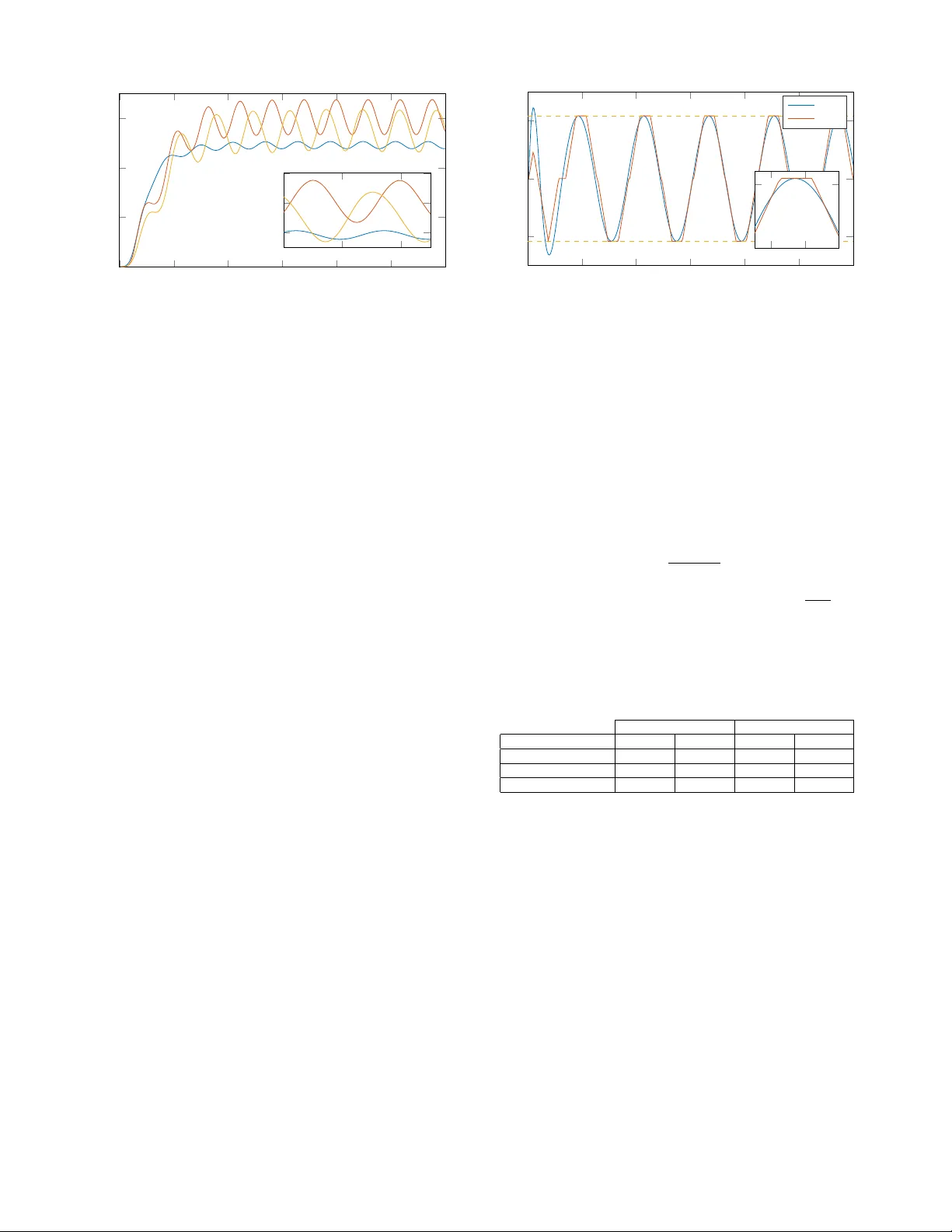
Economic model pr edictiv e contr ol f or snak e r obot locomotion Marko Nonhof f, Philipp N. Köhler , Anna M. Kohl, Kristin Y . Pettersen, and Frank Allgöwer c  2019 IEEE. Personal use of this material is permitted. Permission from IEEE must be obtained for all other uses, in any current or future media, including reprinting/republishing this material for advertising or promotional purposes, creating new collectiv e works, for resale or redistribution to servers or lists, or reuse of any copyrighted component of this w ork in other works. Abstract — In this work, the control of snak e robot loco- motion via economic model predicti ve control (MPC) is studied. Only very few examples of applications of MPC to snake robots exist and rigorous proofs f or recursiv e feasibility and conv er - gence are missing. W e propose an economic MPC algorithm that maximizes the robot’ s forward velocity and integrates the choice of the gait pattern into the closed loop. W e show recursi ve feasibility of the MPC optimization problem, where some of the developed techniques are also applicable for the analysis of a more general class of system. Besides, we provide performance results and illustrate the achieved performance by numerical simulations. W e thereby show that the economic MPC algorithm outperforms a standard lateral undulation controller and achieves constraint satisfaction. Surprisingly , a gait pattern different to lateral undulation results fr om the optimization. I . I N T RO D U C T I O N There has been acti ve research on the mechanisms and control of snake robot locomotion ov er the last decades. As opposed to robots which move in a more traditional way , for example wheeled or legged robots, snake robots carry the potential to not only move in cluttered and irre gular en vironments, but also make use of obstacles to aid in their locomotion. Since the snake robot is a robot manipulator arm that can also locomote, it has a wide range of applications, including firefighting as well as search and rescue tasks. Correspondingly , the scope of research activities ranges from mov ement in tight spaces on land to subsea operations. An ov ervie w over previous literature on modelling, analysis, control and application of snake robots is found in [1]–[3]. The complex dynamics of snake robot locomotion, possi- ble environment interactions, and the presence of constraints on both the input and the states make model predicti ve control (MPC) a promising approach to control the motion of snake robots. MPC is a control method that solves a finite- horizon optimal control problem at e very sampling time instance and applies the first part of the optimal input, see for example [4]. In many applications, setpoint stabilization may not be the primary control objecti ve, but rather optimization of some general performance criterion. For this reason, so called economic MPC was dev eloped, which allo ws to minimize a general performance criterion [5]. Economic MPC has been studied in detail and con vergence, stability , Marko Nonhoff is with the Institute of Automatic Control, Leibniz Univ ersity Hannover , 30167 Hannover , Germany , Philipp N. Köhler and Frank Allgöwer are with the Institute for Systems Theory and Automatic Control, Uni versity of Stuttgart, 70550 Stuttgart, German y . Anna K ohl and Kristin Y . Pettersen are with Centre for Autonomous Marine Operations and Systems (NTNU AMOS), Department of Engineering Cybernetics, Norwe- gian Univ ersity of Science and T echnology , 7491 Trondheim, Norway . and performance results are av ailable for the closed loop (see, e.g., [5]–[8]). It is a well-known property of economic MPC that it can lead to periodic behavior which commonly occurs in snake robot locomotion. Nev ertheless, only very few results exist for applications of MPC to the control of snake robot locomotion. In [9], MPC is emplo yed for path following of a snake robot in terms of optimizing the parameters of a predefined gait pattern. Ho wever , the gait pattern was chosen of fline and no rigorous proofs for recursiv e feasibility of the MPC optimization problem were giv en for the proposed controller . The work at hand de velops a theoretical basis and provides first results on utilizing Model Predictiv e Control techniques for the control of snake robot locomotion without a prede- fined gait pattern. Therefore, we consider a simplified model and assume the snake robot moves on a flat and unbounded surface. In particular , by directly computing the input signals for each joint of the snake robot, the choice of the gait pattern is integrated into the closed loop, as opposed to existing approaches which, e.g., employ feedback controllers to track a predefined gait pattern [1]–[3] or central pattern generators [10]. Thereby , we enable the snake robot to adapt its motion to, e.g., a changing en vironment, faults or changing performance criteria gi ven by an altered cost function. F or simplicity , we focus on maximizing the forward velocity of the snake robot throughout this work, since this yields a simple value function with an intuiti ve physical interpretation and is a reasonable objectiv e of locomotion. Nev ertheless, the central ideas are applicable to more complex stage costs as well. This paper is structured as follo ws: In Section 2, we introduce the mathematical model of the snake robot used in this work and revie w the lateral undulation gait pattern and a corresponding controller from the literature. Section 3 introduces the economic MPC scheme, which is in vestigated analytically regarding recursive feasibility and performance in Section 4. Subsequently , numerical simulations are shown in Section 5, and concluding remarks are giv en in Section 6. Notation: Let I [ a,b ] denote the set of all integers in the interval [ a, b ] ⊂ R , and let I >a denote the set of all integers larger than a ∈ R . d x e is the ceiling function, i.e., d x e = min { n ∈ I | n ≥ x } , and sgn ( x ) represents the signum function. W e consider a discrete-time nonlinear system x ( t + 1) = f ( x ( t ) , u ( t )) , x (0) = x 0 , (1) where f : X × U → R n , x ( t ) ∈ X ⊆ R n and u ( t ) ∈ U ⊆ R m are the system dynamics, the state and the control input at time t ∈ I ≥ 0 , and X and U denote the state and input θ φ i − 1 ( τ i , η i ) ( τ i +1 , η i +1 ) ( τ i − 1 , η i − 1 ) t x y n φ i Fig. 1. Schematic representation of the snake model and the used coordinate systems. constraint sets, respectiv ely . The solution of system (1) for a control sequence u = ( u (0) , . . . , u ( K − 1)) ∈ U K starting at the initial v alue x 0 ∈ X is denoted by x u ( t, x 0 ) , t = 0 , . . . , K , which is abbreviated as x u ( t ) whenev er x 0 is clear from the context. I I . P RO B L E M S E T U P In this section, we present a mathematical model of the snake robot which will be used for controller design, analysis and simulations in the remainder of this work. Modelling a snake robot in full detail yields a dynamical system too complicated for contoller design. For this reason, we will use a simplified model throughout this work, specifically dev eloped for controller design and analysis. A detailed deriv ation of this simplified model can be found in [2], [11]. The main idea is to describe the robot by a serial connection of translational instead of rev olute joints connecting the links of the snake robot, since analysis shows that it is the transversal motion of the links that is significant for forward motion. A schematic representation of the modelling approach is provided in Figure 1. W e consider a planar snak e robot consisting of N l links, all with the same mass m and length l , which are interconnected by N l − 1 translational joints. The center of mass of each link is located at its center point. The robot moves on a horizontal and flat surface and is driven by N l − 1 actuators, one at each joint. First, we define a set of matrices which will be used extensi vely in this work. A = " 1 1 . . . . . . 1 1 # ∈ R ( N l − 1) × N l , D = " 1 − 1 . . . . . . 1 − 1 # ∈ R ( N l − 1) × N l , e = [1 , . . . , 1] T ∈ R N l , e = [1 , . . . , 1] T ∈ R N l − 1 , D = D T  D D T  − 1 ∈ R N l × ( N l − 1) . The matrices A and D represent an addition and sub- traction, respectiv ely , of adjacent elements of a vector . W e assume that the snake robot is subject to an anisotropic viscous ground friction force. More specifically , the ground friction normal to the link is greater than the ground friction parallel to the link. Both for biological snakes and for snake robots, this is the essential feature enabling them to propel forward. W e denote the friction coefficient in normal direction by c n ∈ R > 0 and in tangential direction by c t ∈ R > 0 . Furthermore, we define a propulsion coef ficient c p as c p = c n − c t 2 l . W e are no w ready to state the complete simplified model. As opposed to [2], [11], we give a discretized version, since our MPC scheme will be formulated in discrete-time with sampling time T s . φ ( t + 1) = φ ( t ) + T s v φ ( t ) (2a) θ ( t + 1) = θ ( t ) + T s v θ ( t ) (2b) p x ( t + 1) = p x ( t ) + T s  v t ( t ) cos( θ ( t )) − v n ( t ) sin( θ ( t ))  (2c) p y ( t + 1) = p y ( t ) + T s  v t ( t ) sin( θ ( t )) + v n ( t ) cos( θ ( t ))  (2d) v φ ( t + 1) = v φ ( t ) + T s u ( t ) (2e) v θ ( t + 1) = v θ ( t ) + T s  − λ 1 v θ ( t ) + λ 2 N l − 1 v t ( t ) e T φ ( t )  (2f) v t ( t + 1) = v t ( t ) + T s  − c t m v t ( t ) + 2 c p N l m v n ( t ) e T φ ( t ) − c p N l m φ T ( t ) AD v φ ( t )  (2g) v n ( t + 1) = v n ( t ) + T s  − c n m v n ( t ) + 2 c p N l m v t ( t ) e T φ ( t )  , (2h) where φ ( t ) ∈ R N l − 1 and v φ ( t ) ∈ R N l − 1 denote the joint distances and velocities, ( p x ( t ) , p y ( t )) ∈ R 2 represents the position of the snake robot’ s center of mass in the global frame, v t ( t ) ∈ R and v n ( t ) ∈ R are the tangential and normal velocities of the center of mass in the t − n frame, θ ( t ) ∈ R denotes the orientation and v θ ( t ) ∈ R the snake robot’ s rotational velocity . The parameters λ 1 ∈ R and λ 2 ∈ R are empirical constants which describe the rotational dynamics. A reasonable choice of parameters for this model is presented in [2]. Remark 1: Note that we directly consider the input u ob- tained through an input transformation as sho wn in [2], [11], leading to the simple dynamics (2e). Due to mechanical restrictions of the snake robot and the model only being valid for joint distances φ ( t ) which are sufficiently small [2], state constraints on the joint distances φ ( t ) and the corresponding velocities v φ ( t ) and input constraints need to be respected. These constraints are giv en as box constraints, hence, X = { x ( t ) ∈ R 2 N l +4   φ i ( t ) ∈ [ − φ max , φ max ] , v φ,i ( t ) ∈ [ − v φ, max , v φ, max ] ∀ i ∈ I [1 ,N l − 1] } , (3) U = { u ( t ) ∈ R N l − 1 | u i ( t ) ∈ [ − u max , u max ] ∀ i ∈ I [1 ,N l − 1] } , (4) where x ( t ) = [ φ ( t ) , θ ( t ) , p x ( t ) , p y ( t ) , v φ ( t ) , v θ ( t ) , v t ( t ) , v n ( t )] T , (5) and φ max ∈ R > 0 , v φ, max ∈ R > 0 and u max ∈ R > 0 . W e assume that the remaining states are unconstrained. In [2], [11], a controller was presented which steers the joint distances φ ( t ) to a gi ven reference trajectory , defined by the gait pattern lateral undulation (LU). This gait pattern propagates a body wa ve from head to tail of the snake robot and is defined as φ LU ,i ( t ) = α sin ( ω t + ( i − 1) δ ) , (6) where i ∈ I [1 ,N l − 1] , and α, ω , δ ∈ R are constant parameters. This gait pattern was studied in detail, e.g., in [2], [12]. The corresponding lateral undulation controller is giv en by u ( t ) = u ref ( t ) + k d ( v φ, ref ( t ) − v φ ( t )) + k p ( φ ref ( t ) − φ ( t )) , (7) with φ ref ,i ( t ) = φ LU ,i ( t ) , v φ, ref ,i ( t ) = d d t φ ref ,i ( t ) , u ref ,i ( t ) = d 2 d t 2 φ ref ,i ( t ) . This controller was proven to exponentially stabilize the reference gait pattern for the snake robot model (2). Fur- thermore, in [2], [11] it was shown that the a verage forward velocity con ver ges exponentially fast to a velocity which depends on the parameters describing the gait pattern α, ω , δ and φ 0 , the friction coefficients c n , c t and c p , and the number of links N l . I I I . E C O N O M I C M P C S C H E M E F O R S N A K E RO B O T L O C O M OT I O N As mentioned in the introduction, we aim at maximizing the forward v elocity of the snake robot as a reasonable objectiv e, and in order to arri ve at a simple cost function with an intuiti ve physical interpretation. W e therefore employ − v t ( t ) as the cost to be minimized by the MPC optimization problem. Howe ver , other choices are possible. For instance, in order to limit the energy consumption of the snake robot, a term γ u T ( k | t ) u ( k | t ) with γ ∈ R > 0 could be added (cf. Section V). All our results on recursi ve feasibility provided in the next section are independent of the choice of the specific cost function. Howe ver , our results on the performance of the closed loop would need to be adjusted for a modified cost function. Next, we state our proposed economic MPC algorithm for snake robot locomotion. At each time step t , given an initial value x ( t ) ∈ X , the following MPC optimization problem is solved. Pr oblem 1: (Economic MPC optimization problem) min u ( t ) ∈ U N p J ( x ( t ) , u ( t )) = − N p X k =0 v t ( k | t ) s.t. x (0 | t ) = x ( t ) x ( k + 1 | t ) = f ( x ( k | t ) , u ( k | t )) u ( k | t ) ∈ U ⊆ R N l − 1 k = 0 , . . . , N p − 1 x ( k | t ) ∈ X ⊆ R 2 N l +4 k = 0 , . . . , N p . In Problem 1, the snake robot’ s dynamics f ( x ( k | t ) , u ( k | t )) and states x ( t ) are gi ven by (2) and (5), re- spectiv ely . W e denote the solution to this MPC optimization problem by u ∗ ( t ) = ( u ∗ (0 | t ) , . . . , u ∗ ( N p − 1 | t )) ∈ U N p and the corresponding predicted trajectory by x ∗ ( t ) = ( x ∗ (0 | t ) , . . . , x ∗ ( N p | t )) ∈ X N p +1 , where the asteriks signify optimality . At each timestep, the first element of the optimal input sequence u ∗ ( t ) is applied to the system, hence, the control input is given by u MPC ( t ) = u ∗ (0 | t ) . I V . A NA LY S I S O F T H E C L O S E D L O O P A. Recur sive feasibility Recursiv e feasibility is a fundamental property of MPC algorithms, which is required to apply the MPC scheme to a system. Recursive feasibility means that, if a feasible solution to the MPC optimization problem at time t = t 0 exists, then there is a feasible solution to the problem for ev ery t > t 0 . Hence, recursiv e feasibility establishes that the control law giv en by the above algorithm is defined at all times. In the follo wing, we present a sufficient condition for recursiv e feasibility of Problem 1, which can be achieved without additional terminal costs or constraints, facilitating implementation and, more importantly , not requiring any a priori kno wledge of, e.g., a desirable gait pattern. W e note that the results of this section can be applied to a wider range of problems of similar structure, i.e., systems with box constraints on states adhering to double integrator dynamics. This is discussed in more detail below . The main idea of the following deri vations is to provide a candidate solution to the MPC optimization Problem 1 based on a feasible solution from the previous time step in order to certify that the resulting control input is always defined. Giv en the current state x ( t ) (including v φ ( t ) ), let the input sequence u c ( t ) ∈ U N p and the i -th entry (referring to the i - th joint) of its k -th element u c i ( k | t ) , i ∈ I [1 ,N l − 1] , be defined by the feedback law u c i ( k | t ) = ( − sgn ( v φ,i ( k | t )) u max if | v φ,i ( k | t ) | > T s u max − v φ,i ( k | t ) T s else (8) and let b = d v φ, max T s u max e . (9) Hence, it is always possible to steer v φ ( t ) to zero in b time steps. Let φ ∗ ( t ) = ( φ ∗ (0 | t ) , . . . , φ ∗ ( N p | t )) , v ∗ φ ( t ) = ( v ∗ φ (0 | t ) , . . . , v ∗ φ ( N p | t )) denote the optimal trajectories of the joint distances and ve- locities at time t , respectiv ely . W e define the candidate input sequence ˜ u ( t ) by shifting the previously optimal solution for the first N p − b − 1 time steps and extending it by u c ( t ) , i.e., ˜ u ( t + 1) = ( u ∗ (1 | t ) , . . . , u ∗ ( N p − b − 1 | t ) , u c ( N p − b − 1 | t + 1) , . . . , u c ( N p − 1 | t + 1)) . (10) Remark 2: W e use the candidate input ˜ u ( t ) only for feasibil- ity analysis, and do not intend to actually apply it to the snake robot. When applied to a snake robot, the forward velocity achiev ed with this input would be undesirable, since it steers the joint velocities v φ ( t ) to zero. Therefore, no acceleration can be achieved by body shape changes and the robot is decelerated due to friction. The main idea behind defining this input is that it indeed steers the joint velocities to zero, as will be shown by the next lemma. W e thereby ensure that the states v φ ( t ) and φ ( t ) remain feasible thereafter and only the transient phase of the candidate input sequence u c ( t ) and the corresponding state trajectories remain to be analyzed. In order to prov e the main result of this section, we first examine the response of the joint velocities v u c ( t ) φ ( t ) when actuated by the candidate input sequence u c ( t ) . Namely , we show that the absolute value of v u c φ,i ( t ) is decreasing and its sign does not change if | v φ,i ( t ) | > T s u max . Loosely speaking, this means that the joint velocities are steered towards zero. Lemma 3: Let u c ( t ) be defined by (8). Then it holds that (i) | v φ,i ( k | t ) | ≥ | v u c i φ,i ( k + 1 | t ) | for all i ∈ I [1 ,N l − 1] and k ∈ I [0 ,N p − 1] . (ii) Moreov er , if | v φ,i ( k | t ) | > T s u max , then sgn ( v φ,i ( k | t )) = sgn  v u c i φ,i ( k + 1 | t )  for all i ∈ I [1 ,N l − 1] and k ∈ I [0 ,N p − 1] . Pr oof. (i) Analyzing the dynamics of v φ,i ( k | t ) for some i ∈ I [1 ,N p − 1] and k ∈ I [0 ,N p − 1] giv en by (2e) when applying u c i ( k | t ) yields | v u c i φ,i ( k + 1 | t ) | = | v φ,i ( k | t ) + T s u c i ( k | t ) | . First, assume that | v φ,i ( k | t ) | > T s u max , which gives | v u c i φ,i ( k + 1 | t ) || = | v φ,i ( k | t ) − T s sgn ( v φ,i ( k | t )) u max | < | v φ,i ( k | t ) | . Second, assume otherwise | v φ,i ( k | t ) | ≤ T s u max , which giv es | v u c i φ,i ( k + 1 | t ) || = | v φ,i ( k | t ) − T s v φ,i ( k | t ) T s | = 0 ≤ | v φ,i ( k | t ) | . Combining these two results yields the desired inequality | v φ,i ( k | t ) | ≥ | v u c i φ,i ( k + 1 | t ) | . (ii) Due to | v φ,i ( k | t ) | > T s u max and the def- inition of the input u c i ( k | t ) in (8) it holds that u c i ( k | t ) = − sgn ( v φ,i ( k | t )) u max . Therefore, sgn  v u c i φ,i ( k + 1 | t )  = sgn ( v φ,i ( k | t ) + T s u c i ( k | t )) = sgn ( sgn ( v φ,i ( k | t )) ( | v φ,i ( k | t ) | − T s u max )) = sgn ( v φ,i ( k | t )) . Note that Lemma 3(i) already implies recursiv e feasibility of v φ,i ( k | t ) , i.e., if | v φ,i ( k | t ) | ≤ v φ, max then | v u c i φ,i ( k + 1 | t ) | ≤ | v φ,i ( k | t ) | ≤ v φ, max . Next, we state the main result of this section. It provides a sufficient condition for recursive feasibility of Problem 1. The only required assumption is existence of an initially feasible input at time t = t 0 as is standard in MPC feasibility analysis. Lemma 4: Suppose that there e xists an initially feasible solution u ∗ ( t ) to Problem 1 at time t = t 0 . If N p > b , then there exists a feasible solution to Problem 1 for all t ∈ I >t 0 . Pr oof. W e assume that Problem 1 was feasible at time t . Then, it has to be shown that the input constraint (4) and both state constraints (3) can be satisfied at time t + 1 . As common in MPC, this is done by showing feasibility of a suboptimal candidate trajectory , which in our case results from application of the candidate input sequence (10). First, we examine the input constraint. For the first N p − b − 1 time steps the candidate input sequence ˜ u ( t + 1) is feasible since it is the same as the shifted optimal input u ∗ ( t ) which is feasible by assumption. For the remaining time steps, the candidate input sequence is feasible, since u c i ( k | t ) is either defined by | u c i ( k | t + 1) | = | − sgn ( v φ,i ( k | t + 1)) u max | ≤ u max or by | u c i ( k | t + 1) | = | − v φ,i ( k | t + 1) T s | ≤ | T s u max | T s = u max . It follo ws that the candidate input trajectory satisfies the input constraints for all k ∈ I [0 ,N p − 1] . Second, we in vestigate the response of the joint velocities v φ ( k | t + 1) to the candidate input sequence. For the first N p − b steps it holds that the constraint on v ˜ u φ ( k | t + 1) is satisfied, since the solution of Problem 1 at time t is feasible and, by the construction of the candidate input sequence (10), the resulting trajectories are the same. F or the remaining time steps, constraint satisfaction is provided by Lemma 3(i). Finally , we examine the response of the joint distances φ ( k | t + 1) to the candidate input. For notational conv enience, we define b = N p − b . Again, by the construction of the candidate input sequence (10), the trajectory is the same as the optimal trajectory for the first N p − b + 1 time steps. φ ˜ u ( k | t + 1) = φ ∗ ( k + 1 | t ) , k ∈ I [0 ,N p − b ] . For the remaining time steps, we obtain p ∈ I [1 ,b ] and φ ˜ u ( b + p | t + 1) = φ ˜ u ( b − 1 + p | t + 1) + T s v ˜ u φ ( b − 1 + p | t + 1) , and by recursi vely inserting the system dynamics, first (2a) and then (2e), = φ ∗ ( b + 1 | t ) + T s p X q =1 v ˜ u φ ( b − 1 + q | t + 1) (11) = φ ∗ ( b + 1 | t ) + T s p X q =1 v ∗ φ ( b | t ) + T s q X r =1 u c ( b − 2 + r | t + 1) ! . (12) Again, the first N p − b + 1 time steps are feasible because the candidate input sequence ˜ u ( t + 1) is the same as the previously feasible solution u ∗ ( t ) . The main idea of proving feasibility of the remaining time steps is to bound the candidate joint distances by the previously feasible trajectory . In the following, we need to consider three different cases, depending on the candidate input u c ( k | t ) . In the first two cases, we compare the candidate trajectory directly to the previously feasible trajectory of the joint distances. In the third case, we sho w feasibility by induction. First, assume v ˜ u φ,i ( b − 2 + p | t + 1) > T s u max for some p ∈ I [1 ,b ] which implies v ˜ u φ,i ( b − 2 + r | t + 1) > T s u max > 0 and u c i ( b − 2 + r | t + 1) = − u max ≤ u ∗ i ( b − 1 + r | t ) for all r ∈ I [1 ,p ] by Lemma 3 and also v ˜ u φ,i ( b − 1 + p | t + 1) > 0 due to Lemma 3(ii). Then, inserting (12) yields φ ˜ u i ( b + p | t + 1) = φ ∗ i ( b + 1 | t ) + T s p X q =1 v ∗ φ,i ( b | t ) + T s q X r =1 u c i ( b − 2 + r | t + 1) ! ≤ φ ∗ i ( b + 1 | t ) + T s p X q =1 v ∗ φ,i ( b | t ) + T s q X r =1 u ∗ i ( b − 1 + r | t ) ! = φ ∗ i ( b + 1 + p | t ) ≤ φ max and, by inserting (11), φ ˜ u i ( b + p | t + 1) = φ ∗ i ( b + 1 | t ) + T s p X q =1 v ˜ u φ,i ( b − 1 + q | t + 1) >φ ∗ i ( b + 1 | t ) ≥ − φ max . Second, if v ˜ u φ,i ( b − 2 + p | t + 1) < − T s u max , the arguments are the same as abov e and are therefore omitted. Third, if | v ˜ u φ,i ( b − 2 + p | t + 1) | ≤ T s u max holds, which implies u c i ( b − 2 + p | t + 1) = − 1 T s v ˜ u φ,i ( b − 2 + p | t + 1) , then the joint distance φ ˜ u i ( b + p | t + 1) remains constant and, hence, feasible by induction: φ ˜ u i ( b + p | t + 1) = φ ˜ u i ( b − 1 + p | t + 1) + T s v ˜ u φ,i ( b − 2 + p | t + 1) + T 2 s u c i ( b − 2 + p | t + 1) = φ ˜ u i ( b − 1 + p | t + 1) . Combining these three results yields feasiblity for all elements of the sequence φ ˜ u ( t + 1) except for the last one. Hence, it only remains to sho w that the last element φ ˜ u ( N p | t + 1) of the sequence is feasible. If v ˜ u φ ( N p − 1 | t +1) = 0 then φ ˜ u ( N p | t + 1) = φ ˜ u ( N p − 1 | t + 1) would be feasible as sho wn abov e. In the follo wing, we show that indeed v ˜ u φ ( N p − 1 | t + 1) = 0 holds, by a contradiction argument to feasibility of the previous solution u ∗ ( t ) . First, assume otherwise v ˜ u φ,i ( N p − 1 | t + 1) 6 = 0 for some i ∈ I [1 ,N l − 1] . If v ˜ u φ,i ( N p − 2 | t + 1) = 0 , then u c i ( N p − 2 | t + 1) = 0 holds and thus v ˜ u φ,i ( N p − 1 | t + 1) = 0 , which is a contradiction. Hence, v ˜ u φ,i ( N p − 2 | t + 1) 6 = 0 . If | v ˜ u φ,i ( N p − 2 | t + 1) | ≤ T s u max , then, by (8), u c i ( N p − 2 | t + 1) = − 1 T s v ˜ u φ,i ( N p − 2 | t + 1) which yields v ˜ u φ,i ( N p − 1 | t + 1) = 0 due to (2e). Again, this is a contradiction, so | v ˜ u φ,i ( N p − 2 | t + 1) | > T s u max . Moreov er , if v ˜ u φ,i ( N p − 2 | t + 1) > T s u max then this is also true for ev ery time step before where u c i ( k | t + 1) was applied, due to Lemma 3. Furthermore, this implies v ˜ u φ,i ( N p − 1 | t + 1) > 0 because of Lemma 3(ii). Repeatedly inserting the system dynamics (2e) into this equation yields 0 < v ˜ u φ,i ( N p − 1 | t + 1) = v ∗ φ,i ( N p − b − 1 | t ) + T s b X q =1 u c i ( N p − b − 2 + q | t + 1) = v ∗ φ,i ( N p − b − 1 | t ) − T s bu max ≤ v ∗ φ,i ( N p − b − 1 | t ) − v φ, max ⇒ v φ, max < v ∗ φ,i ( N p − b − 1 | t ) , which is a contradiction to feasibility of the optimal solution at time t . Lastly , if v ˜ u φ,i ( N p − 2 | t + 1) < T s u max the same contradiction to feasibility of the optimal solution is achiev ed by the same arguments. Hence, v ˜ u φ,i ( N p − 1 | t + 1) = 0 and φ u di,i ( N p | k + 1) = φ ˜ u ( N p − 1 | t + 1) which concludes the proof. Remark 5: Note that in this proof we only in vestigated the constrained states φ ( t ) , v φ ( t ) and the input u ( t ) , which adhere to double integrator dynamics. Neither the additional states nor the cost function enter our analysis. This result can therefore be applied to any system with constraints on a double integrator subsystem, possibly additional uncon- strained states and an arbitrary cost function, which is found in many different kinds of mobile robot applications. B. P erformance guarantees In this section, we briefly discuss performance guaran- tees for the proposed economic MPC scheme in terms of achieving a certain benchmark velocity . Howe ver , a thorough presentation of our results is out of the scope of this paper . The analysis in this section is tailored to an economic MPC scheme which aims to maximize the snake robot’ s forward velocity . In the following, the cost function in Problem 1 is therefore chosen as J ( x ( t ) , u ( t )) = − P N p k =0 v t ( k | t ) , as discussed in the previous sections. Hence, the results in this section w ould need to be adapted for a dif ferent cost function. In the literature, con vergence to an optimal periodic orbit for economic MPC schemes is usually shown by exploiting certain dissipativity properties of the system; see for instance [5], [7], [13]. Due to the complexity of the snake robot model, showing such a dissipativity seems not to be possible. Instead, we assume existence of an auxiliary controller, which can suf ficiently accelerate the snake robot, and yields a cost which is upper bounded. This is detailed belo w . Moreov er , to properly state our result below , we additionally need to make the reasonable assumption that the economic MPC scheme will keep a certain velocity lev el once it has reached it. More precisely , let v t ( t ) be the current velocity and let ˜ v t ∈ R be a benchmark forward velocity used for performance characterization. Then, we assume that the set { x ( t ) ∈ X | v t ( t ) ≥ ˜ v t } is forward in variant under the proposed economic MPC scheme. Assumption 6: Define V = { x ( t ) ∈ X | v t ( t ) ≥ ˜ v t } , where ˜ v t ∈ R > 0 . Then, the set V is in variant in the economic MPC closed loop. Moreov er , for a given sampling time T s ∈ R > 0 , denote by  ∈ R the solution of  := max x ( t ) ∈ X 1 T s ( v t ( t ) − v t ( t + 1)) . This constant  is a measure for ho w much the snake robot can slow down from one time step to the next, i.e., v t ( t + 1) ≥ v t ( t ) − T s  holds for all x ( t ) ∈ X . Note that it is independent of u ( t ) , since the input does not directly enter the dynamics of the forward velocity v t ( t + 1) , if we in vestigate only one time step. Assumption 7: Let ˜ v t ∈ R > 0 . There exists some 1 β ∈ KL , such that for ev ery x ( t ) ∈ X with v t ( t ) < ˜ v t there exists an input sequence ¯ u ( t ) ∈ U N p which satisfies ˜ v t − v ¯ u t ( t + k 1 ) ≤ β ( ˜ v t − v t ( t ) , k 1 ) , k 2 X i =1 v ¯ u t ( t + i ) ≥ mv t ( t ) − T s , 1 A continuous function β : R ≥ 0 × R ≥ 0 → R ≥ 0 is said to be of class KL if β ( · , t ) is strictly increasing, β (0 , t ) = 0 , and β ( r, · ) is decreasing with lim k →∞ β ( r , k ) = 0 , cf. [14]. for all k 1 ∈ I [0 ,N p ] and for all k 2 ∈ I [1 ,N p ] . Assumption 7 can be justified by in vestigating the closed- loop trajectory of the forw ard velocity when applying the standard lateral undulation controller gi ven by (7). Combining these two assumptions yields the desired per- formance result, i.e., con vergence of the closed loop to the set V . Hence, the application of the proposed economic MPC scheme leads to an acceleration sufficient to reach the velocity ˜ v t and, once it is achieved, remains greater than this benchmark velocity . Lemma 8: Let Assumptions 6 and 7 hold and assume that Problem 1 is initially feasible at time t = t 0 with N p > b . Then, Problem 1 is feasible for all t ∈ I ≥ t 0 and the closed loop con ver ges to the set V . The proof of Lemma 8 is omitted in this paper . All details can be found in [15]. Summarizing, we gi ve performance guarantees for the economic MPC closed-loop snake robot system which are based on assumptions that can be justified, e.g., by simulations of existing standard controllers. V . N U M E R I C A L S I M U L ATI O N S Having established recursiv e feasibility , we demonstrate the ef fectiv eness of the proposed economic MPC scheme and compare it to a standard lateral undulation controller through numerical simulations. Our proposed ecnomic MPC algorithm was implemented in CasADi [16]. For the sake of comparability we choose to use a similar set of parameters as in [2], [9], and [11]. The snake robot’ s N l = 9 links all hav e the same mass m = 1 kg, the same length l = 0 . 14 m and friction coefficients in normal and tangential direction c n = 3 and c t = 1 , respectiv ely . W e set t 0 = 0 s and initialize the snake robot with φ (0) = [0 , 0 . 01 , − 0 . 01 , 0 . 01 , 0 , 0 , 0 . 01 , − 0 . 01] T m, v φ (0) = 0 m/s, v t (0) = 0 m/s and v n (0) = 0 m/s. The sampling time is chosen as T s = 0 . 05 s and the prediction horizon is set to N p = 20 which is equiv alent to 1 s. Finally , the constraint sets are giv en as φ max = 0 . 052 m , v φ, max = 0 . 109 m/s , u max = 0 . 2276 m/s 2 . In order to confirm recursi ve feasibility we verify the conditions of Lemma 4 and obtain b = 10 < N p = 20 from (9). Hence, the ecnomic MPC scheme is feasible for all t ∈ I > 0 , since it is easy to see that it is initially feasible at t = 0 for u (0) = (0 , . . . , 0) . For comparison, we consider the standard lateral undulation controller (7) which is taken from [2], [11]. The lateral undulation gait pattern parameters and the tuning parameters of the controller are adjusted such that it fully utilizes the entire constraint sets once it periodically applies the lateral undulation gait pattern and reaches a high asymptotic av erage forward velocity . Therefore, the gait pattern parameters are chosen as α = 0 . 05 m, ω = 120 deg/s, δ = 40 deg and φ 0 = 0 m. The tuning 0 50 100 150 200 250 300 0 2 4 6 · 10 − 2 T ime Steps (1/20 s) Forward V elocity v t (m/s) 160 180 200 5 6 7 · 10 − 2 Fig. 2. Closed-loop trajectories of the forward velocity v t ( t ) for lateral undulation (blue) and the economic MPC scheme for values of γ = 0 (red) and γ = 0 . 025 (yellow). parameters of the controller are taken from [2], [11] and are set to k d = 5 1/s and k p = 20 1/s 2 . A. Economic MPC vs. Lateral Undulation In the following, we first compare the velocity achie ved by both controllers, i.e., the economic MPC scheme and the standard lateral undulation controller . Additionally , we highlight belo w the ability of our proposed economic MPC approach to incorporate arbitrary objectiv es in the optimiza- tion by accounting for energy consumption in the objective function, and again, compare it to the standard lateral undu- lation controller . In the following, we set the cost function in the eco- nomic MPC optimization Problem 1 to J ( x ( t ) , u ( t )) = P N p k =0 − v t ( k | t ) + γ u T ( k | t ) u ( k | t ) , where γ ∈ R ≥ 0 . Here, the term γ u T ( k | t ) u ( k | t ) accounts for consumed energy , which is inv estigated below . W e compare the proposed economic MPC algorithm for two dif ferent values of γ with the standard lateral undulation controller . In the first experiment, we choose γ = 0 , which yields the cost function analyzed in Section IV -B, and in the second experiment, we choose γ = 0 . 025 , which means that energy consumption is taken into account in the optimization. Figure 2 sho ws the resulting closed-loop forward velocity for the lateral undulation controller giv en by (7) and the economic MPC scheme. One can identify a transient phase until approximately 100 time steps and a periodic orbit afterwards. The asymptotic av erage velocity achie ved by economic MPC for both values of γ is clearly superior to lateral undulation. This is achieved by a more efficient gait pattern: In Figure 3, the trajectories of the joint v elocities of joint 3 are illustrated together with the corresponding constraint ± v φ, max for both controllers. Surprisingly , a gait pattern different to lateral undulation emerges from economic MPC. Instead of a sinusoid as in lateral undulation, the pro- posed controller leads to an approximately piece-wise linear trajectory which results in the observed performance gain. Moreov er , the economic MPC scheme achiev es constraint satisfaction while the lateral undulation controller violates 0 50 100 150 200 250 300 − 0 . 1 0 0 . 1 T ime Steps (1/20 s) Joint V elocity v φ, 3 (m/s) LU EMPC 160 170 180 0 0 . 1 Fig. 3. Closed-loop trajectories v φ,i ( t ) for i = 3 and constraints ± v φ, max for γ = 0 and lateral undulation. the constraints during the transient phase, which explains the qualitativ ely different closed-loop forward velocity during the first 50 time steps. The superior velocity comes at the price of an increased energy consumption, which is in vestigated next. In order to compare the asymptotic av erage energy consumption and for - ward velocity , we computed the average energy consumption and velocity over the last 200 time steps of our simulations. W e consider E = P 300 t =100 u T ( t ) u ( t ) 200 as a measure for the consumed energy by the controllers, while the asymptotic av erage velocity is computed by v av = P 300 t =100 v t ( t ) 200 . The results of this comparison are giv en in T able I. T ABLE I C O MPA R IS O N O F T H E A S Y MP T OT I C A V E R AG E E N E R GY CO N S U MP T I O N A N D F O RW A R D V E LO C I TY Energy E A vg. velocity v av Gait pattern absolute relativ e absolute relativ e LU 0 . 2072 100 . 0% 0 . 0494 100% EMPC, γ = 0 0 . 2624 126 . 6% 0 . 0609 123 . 3% EMPC, γ = 0 . 025 0 . 1979 95 . 5% 0 . 0554 112 . 1% The data demonstrates that the economic MPC algorithm reaches a higher asymptotic av erage forward velocity in both cases, while it simultaneously leads to a lower energy consumption if the value of γ is tuned to take energy consumption into account. Hence, the adv antage of the proposed economic MPC scheme is twofold: It achie ves a higher performance in terms of forward velocity as well as in terms of energy consumption by finding a superior gait pattern while ensuring constraint satisfaction. B. Actuator fault W e next in vestigate the case of a joint failure occuring during operation to specifically illustrate the advantage of integrating the choice of the gait pattern into the closed loop. W e simulate the scenario of joint 4 blocking after 10 s, and we therefore fix v φ, 4 ≡ 0 m/s afterwards. For this experiment, we set γ = 0 in the cost function and 0 100 200 300 400 500 0 2 4 6 · 10 − 2 T ime Steps (1/20 s) Forward V elocity v t (m/s) fault-aware fault-unaware Fig. 4. Closed-loop trajectories v t ( t ) for the economic MPC scheme with and without information about the actuator fault. compare an economic MPC algorithm which has access to information about the failure, i.e., where we set v φ, 4 ≡ 0 m/s and u 4 ≡ 0 m/s 2 in the dynamic constraints in Problem 1, with a fault-unaware economic MPC scheme. Figure 4 sho ws the resulting closed-loop velocity for both controllers. It can be observed, that the fault-aw are controller achiev es a slightly higher asymptotic average velocity after the failure has occured. Computing the a verage velocity as in the previous subsection by v av = P 500 t =300 v t ( t ) 200 yields 0 . 0435 m/s for the algorithm with access to information about the failure and 0 . 0418 m/s for the fault-unaw are algorithm. Moreov er , in Figure 5 the corresponding joint distances for joint i = 3 are illustrated. It becomes apparent that the economic MPC scheme adapts the gait pattern once the failure occurs in order to reach a higher forward velocity . V I . C O N C L U S I O N In this work, we proposed an economic MPC scheme for snake robot locomotion that integrates the choice of the gait pattern into the closed loop. W e prov ed recursiv e feasibility of the economic MPC scheme in the closed loop and briefly sketched performance guarantees. W e compared the proposed economic MPC algorithm to a standard lateral undulation controller from the literature and demonstrated that economic MPC is able to improve the snak e robot’ s performance in terms of velocity and energy consumption at the same time, while ensuring constraint satisfaction. The theoretical foundations and insights gained by this work serve as a first step towards applying MPC to the control of snake robot locomotion with different performance criteria, subject to additional constraints and in the presence of obstacles. W e belie ve that the ability to implicitly choose a gait pattern online through the economic MPC algorithm will be particularly beneficial for utilizing obstacles for locomotion, which is part of our ongoing work. R E F E R E N C E S [1] P . Liljebäck, K. Y . Pettersen, Ø. Stavdahl, and J. T . Gravdahl, “ A revie w on modelling, implementation, and control of snake robots, ” Robotics and Autonomous Systems , v ol. 60, no. 1, pp. 29–40, 2012. 0 100 200 300 400 500 − 5 0 5 · 10 − 2 T ime Steps (1/20 s) Joint Distance φ 3 (m) fault-aware fault-unaware Fig. 5. Closed-loop trajectories φ 3 ( t ) for the economic MPC scheme with and without information about the actuator fault. [2] P . Liljebäck, K. Y . Pettersen, Ø. Stavdahl, and J. T . Gravdahl, Snake Robots - Modelling, Mechatronics, and Contr ol . Berlin Heidelberg: Springer Science & Business Media, 2012. [3] K. Y . Pettersen, “Snake robots, ” Annual Reviews in Control , vol. 44, pp. 19 – 44, 2017. [4] J. B. Rawlings and D. Q. Mayne, Model Pr edictive Contr ol - Theory and Design . Nob Hill Pub ., 2009. [5] M. A. Müller and F . Allgöwer, “Economic and distributed model predictiv e control: Recent developments in optimization-based con- trol, ” SICE J ournal of Contr ol, Measurement, and System Inte gration , vol. 10, no. 2, pp. 39–52, 2017. [6] M. Ellis, H. Durand, and P . D. Christofides, “ A tutorial review of economic model predicti ve control methods, ” Journal of Pr ocess Contr ol , vol. 24, no. 8, pp. 1156–1178, 2014. [7] D. Angeli, R. Amrit, and J. B. Rawlings, “On average performance and stability of economic model predictive control, ” IEEE Tr ansactions on Automatic Contr ol , vol. 57, no. 7, pp. 1615–1626, 2012. [8] M. A. Müller and L. Grüne, “Economic model predictive control with- out terminal constraints for optimal periodic behavior , ” Automatica , vol. 70, pp. 128–139, 2016. [9] G. Marafioti, P . Liljebäck, and A. Transeth, “ A study of nonlinear model predictive control (NMPC) for snake robot path following, ” in Proc. of the IEEE International Confer ence on Robotics and Biomimetics , pp. 568–573, 2014. [10] A. J. Ijspeert, “Central pattern generators for locomotion control in animals and robots: A revie w , ” Neural Networks , vol. 21, no. 4, pp. 642 – 653, 2008. [11] P . Liljebäck, K. Y . Pettersen, Ø. Stavdahl, and J. T . Gravdahl, “Lateral undulation of snake robots: A simplified model and fundamental properties, ” Robotica , vol. 31, pp. 1005–1036, 2013. [12] M. Sato, M. Fukaya, and T . Iwasaki, “Serpentine locomotion with robotic snakes, ” IEEE Contr ol Systems Magazine , vol. 22, no. 1, pp. 64–81, 2002. [13] M. A. Müller, L. Grüne, and F . Allgöwer, “On the role of dissipativity in economic model predicti ve control, ” in Proc. of the 5th IF AC Confer ence on Nonlinear Model Pr edictive Contr ol , vol. 48, pp. 110– 116, 2015. [14] H. K. Khalil, Nonlinear Systems . New Y ork: Pearson Education, 2013. [15] M. Nonhoff, “Economic and distributed MPC for snake robot loco- motion, ” Master’ s thesis, Institute for Systems Theory and Automatic Control, Univ ersity of Stuttgart, 2018. [16] J. A. E. Andersson, J. Gillis, G. Horn, J. B. Rawlings, and M. Diehl, “CasADi: a software framew ork for nonlinear optimization and opti- mal control, ” Mathematical Pr ogramming Computation , 2018.