A Computationally Efficient Neural Network Invariant to the Action of Symmetry Subgroups

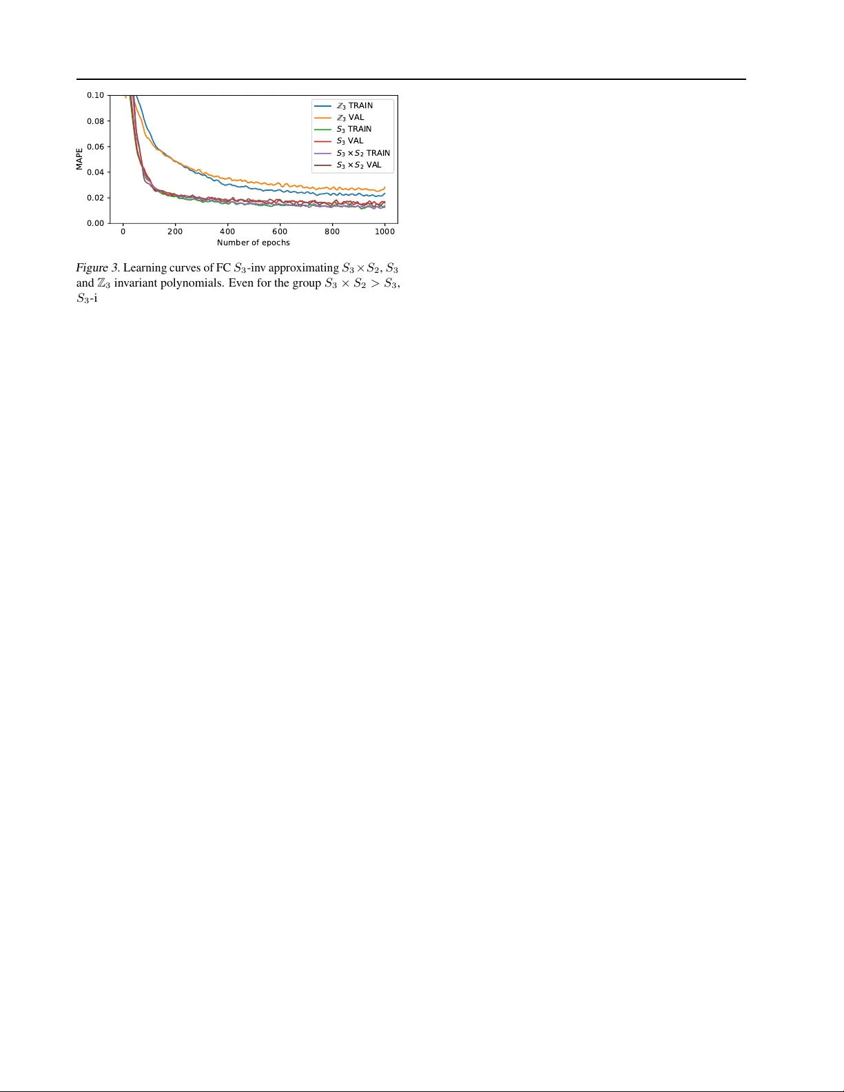
A Computationally Efficient Neural Network In variant to the Action of Symmetry Subgr oups Piotr Kicki † Mete Ozay Piotr Skrzypczyski † Abstract W e introduce a method to design a computation- ally ef ficient G -in v ariant neural netw ork that ap- proximates functions in v ariant to the action of a giv en permutation subgroup G ≤ S n of the symmetric group on input data. The ke y element of the proposed network architecture is a new G -in v ariant transformation module, which pro- duces a G -in v ariant latent representation of the input data. This latent representation is then pro- cessed with a multi-layer perceptron in the net- work. W e pro ve the uni versality of the proposed architecture, discuss its properties and highlight its computational and memory efficiency . Theo- retical considerations are supported by numerical experiments in volving different netw ork configu- rations, which demonstrate the ef fecti veness and strong generalization properties of the proposed method in comparison to other G -in v ariant neural networks. 1. Introduction The design of probabilistic models which reflect symmetries existing in data is considered an important task following the notable success of deep neural networks, such as con volu- tional neural networks (CNNs) ( Krizhe vsk y et al. , 2012 ) and PointNet ( Qi et al. , 2016 ). Using prior knowledge about the data and expected properties of the model, such as permu- tation in v ariance ( Qi et al. , 2016 ), one can propose models that achiev e superior performance. Similarly , translation equiv ariance can be exploited for CNNs ( Cohen & W elling , 2016a ) to reduce their number of weights. Nev ertheless, researchers hav e been working on de veloping a general approach which enables to design architectures that are in v ariant and equi v ariant to the action of particular groups G . In v ariance and equi v ariance of learning models to actions of v arious groups G are discussed in the literature ( Zaheer et al. , 2017 ; Cohen et al. , 2019 ; Ravanbakhsh et al. , † Institute of Robotics and Machine Intelligence, Poznan Uni- versity of T echnology , Poznan, Poland. Correspondence to: Piotr Kicki < piotr .z.kicki@doctorate.put.poznan.pl > . G-invariant neural network Γ  = ( 1 2 3 4 ) [     ]             Γ ( [     ] ) =  1 Γ ( [     ] ) =  2 Γ ( [     ] ) =  1 [     ] [     ] Figure 1. An illustration of employment of the proposed G - in v ariant neural network Γ for estimation of area of quadrangles. No matter which vertex of a quadrangle [ A B C D ] is gi v en first, if the consecuti v e vertices are pro vided in the same order (e.g. for the quadrangle [ C D B A ] ), then the network Γ computes the same area P 1 . Howe ver , the network Γ is not inv ariant to all permuta- tions. For example, the shape of [ A C B D ] is hourglass-like, and the order of its v ertices is dif ferent from that of the other quad- rangles. Therefore, the network Γ estimates a different area P 2 (please see the examples in the yello w boxes). 2017 ). Howe v er , in this paper, we only consider in variance to permutation groups G , which are the subgroups 1 of the symmetric group S n of all permutations on a finite set of n elements, as it cov ers many interesting applications. An example of the employment of the proposed G -in v ariant network for a set of quadrangles is illustrated in Figure 1 . The network Γ receiv es a matrix representation of the quad- rangles (i.e. a vector of 4 points on a plane) and outputs the areas cov ered by those quadrangles. One can spot that, no matter which point will be giv en first, if the consecuti v e verte xes are pro vided in the right order , t he area of the figure will remain the same. Such property can be described as G -in v ariance, where G = (1234) 2 . Recently , Maron et al. ( 2019b ) proposed a G -in v ariant neu- ral network architecture for some finite subgroups G ≤ S n and proved its univ ersality . Unfortunately , their proposed solution is intractable for larger inputs and groups, because of the rapidly growing size of tensors and the number of 1 A subset G ⊂ S n is a subgroup of S n if and only if it satis- fies group properties. Please see the appendix A for the formal definitions. 2 G = (1234) denotes a group G generated by the permutation (1234) , in which the first element is replaced by the second, second by the third and so on, till last element being replaced by first. A Computationally Efficient Neural Network In v ariant to the Action of Symmetry Subgroups operations needed for forward and backward passes in the network. The aim of this paper is to propose a method that enables us to design a nov el G -in v ariant architecture for a gi v en finite group G ≤ S n , which is uni v ersal, able to generalize well and tractable ev en for big groups. The paper is organized as follows: 1. Related work is gi v en in Section 2 . 2. In Section 3.1 , we introduce our G -in v ariant network architecture, which consists of (i) a G -in v ariant transfor - mation block composed of a G -equiv ariant network and a Sum-Product Layer (SPL) denoted by ΣΠ which em- ploys a superposition of product units ( Durbin & Rumel- hart , 1989 ), and (ii) a fully connected neural network. 3. In Section 3.2 , we elucidate the in v ariance of the pro- posed network to the actions of hierarchical subgroups. For this purpose, we describe the cases when the pro- posed G -in v ariant network can be also H -in v ariant for G < H ≤ S n . 4. In Section 3.3 , we prov e that any continuous G -in v ariant function f : V → R , where V is a compact subset of R n × n in , for some n, n in > 0 , can be approximated using the proposed G -in v ariant network architecture. 5. In Section 3.4 , we discuss in detail the computational effi- ciency of the proposed method and relate that to the state- of-the-art G -in v ariant architecture proposed by Maron et al. ( 2019b ). 6. In Section 4 , we pro vide experimental analyses and nu- merical ev aluation of the proposed method and state-of- the-art G -in v ariant neural networks on two benchmark tasks: (i) G -in v ariant polynomial approximation and (ii) conv ex quadrangle area estimation. Moreover , we examine e xperimentally scalability , robustness and com- putational efficienc y of the models learned using the proposed G -in v ariant networks. 7. In Section 5 , we summarize the paper and provide a detailed discussion. 2. Related W ork In order to make use of symmetry properties of data while learning deep feature representations, various G -in v ariant or G -equiv ariant neural networks hav e been proposed in the last decade. In various tasks, learned network models should rev eal the inv ariance or equiv ariance to the whole group S n of all permutations on a finite set of n -elements. Qi et al. ( 2016 ) applied a permutation in v ariant network for point cloud processing, whereas Zaheer et al. ( 2017 ) applied both in v ariant and equi v ariant networks on sets. A permuta- tion equiv ariant model was used by Hartford et al. ( 2018 ) to model interactions between two or more sets. For this pur - pose, they proposed a method to achiev e permutation equiv- ariance by parameter sharing. ( Lee et al. , 2019 ) proposed an approach to achie ve in variance to all permutations of input data utilizing an attention mechanism. Another popular use case of S n -in v ariance and equi v ariance properties are neu- ral networks working on graphs, which were discussed in Keri ven & Peyr ´ e ( 2019 ) and Maron et al. ( 2019a ). Although the aforementioned papers present interesting approaches to obtain in v ariance to all permutations, the approach proposed in our paper allo ws to induce more general in variance to any subgroup of the symmetric group S n . G -equiv ariant neural networks, where G is not a subgroup of S n , are considered by Cohen & W elling ( 2016b ) and Cohen et al. ( 2019 ). G -equiv ariant Con v olutional Neural Networks on homogeneous spaces were discussed by Cohen et al. ( 2019 ), whereas Cohen & W elling ( 2016b ) considered modeling in v ariants to actions of the groups on images, such as to image reflection and rotation. Recent works hav e studied in v ariants to some specific finite subgroups G of the symmetric group S n , which is also con- sidered in this paper . An approach exploiting the parameter sharing for achie ving the in variant and equi v ariant models to such group actions was introduced by Rav anbakhsh et al. ( 2017 ). Maron et al. ( 2019b ) used a linear layer model to compute a G -in v ariant and equi v ariant uni v ersal approxima- tion function. Howe ver , their proposed solution requires the use of high dimensional tensors, which can be intractable for larger inputs and groups. In turn, Y arotsk y ( 2018 ) con- sidered provably univ ersal architectures that are based on polynomial layers, but he assumed that the generating set of G -in v ariant polynomials is gi ven, which is rather imprac- tical. Moreover , there is also a simple approach to achie ve G -in v ariance of an y function, which e xploits a veraging of outputs of functions ov er a whole group G ( Derksen & Kem- per , 2002 ), but it linearly increases the overall number of computations with the size of the group. The approach proposed in this paper builds on the work of Y arotsky ( 2018 ) and provides a netw ork architecture to perform end-to-end tasks requiring G -in v ariance using a tractable number of parameters and operations, utilizing product units ( Durbin & Rumelhart , 1989 ) with Re ynolds operator ( Derksen & K emper , 2002 ). While our approach is not dedicated to image processing and computer vision tasks, it can be used to construct G -in v ariant netw orks for different types of structured data that do not necessarily hav e temporal or sequential ordering (e.g. geometric shapes and graphs). This makes the proposed architecture useful in geometric deep learning ( Bronstein et al. , 2017 ), and in a wide area of applications, from robotics to molecular biol- ogy and chemistry , where it can be used e.g. for estimating the potential energy surfaces of the molecule ( Braams & Bowman , 2009 ; Li et al. , 2013 ). A Computationally Efficient Neural Network In v ariant to the Action of Symmetry Subgroups 3. G -in variant Network In this section, we introduce a novel G -in v ariant neural network architecture, which exploits the theory of inv ari- ant polynomials and the uni v ersality of neural networks to achiev e a flexible scheme for G -in v ariant transformation of data for some known and finite group G ≤ S n , where S n is a symmetric group and | G | = m . Next, we discuss in v ariance of networks to actions of groups with a hierar- chical structure, such as in v ariance to actions of groups H , where G < H ≤ S n . Then, we prov e the uni versality of the proposed method and finally analyze its computational and memory complexity . 3.1. G -in variant Netw ork Ar chitecture W e assume that an input x ∈ R n × n in to the proposed network is a tensor 3 x = [ x 1 x 2 . . . x n ] T of n vectors x i ∈ R n in , i = 1 , 2 , . . . , n . The G -in v ariance property of a function f : R n × n in → R means that f satisfies ∀ x ∈ R n × n in ∀ g ∈ G f ( g ( x )) = f ( x ) , (1) where 4 the action of the group element g on x is defined by g ( x ) = { x σ g (1) , x σ g (2) , . . . , x σ g ( n ) } , (2) where x σ g ( i ) ∈ R n in and σ g ( i ) represents the action of the group element g on the specific index i . Similarly , a function f : R n × p → R n × q has a G -equiv ariance property , if the function f satisfies ∀ g ∈ G ∀ x ∈ R n × p g ( f ( x )) = f ( g ( x )) . (3) G-equivariant function    Sum-Product Layer Σ Π Multi Layer Perceptron      Input G-invariant transformation Γ (  ) Output G - in v a r ia n t f u n c tio n Γ (  ) ℝ  ×    ℝ  ×  ×     ℝ     ℝ     Figure 2. An illustration of the proposed G -in v ariant neural net- work. Input x is processed by the G -in v ariant transformation (blue), which produces G -in v ariant representation of the input. Then, the G -in v ariant representation is passed to the Multi Layer Perceptron which produces the output vector Γ( x ) . The proposed G -in v ariant neural network is illustrated in Figure 2 and defined as function Γ : R n × n in → R n out of the following form Γ( x ) = f out (ΣΠ( f in ( x ))) , (4) 3 W e use matrix notation to denote tensors in this paper . 4 ∀ y ∈ Y P ( Y ) means that “predicate P ( Y ) is true for all y ∈ Y ”. where f in is a G -equiv ariant input transformation function, ΣΠ is a function which, when combined with f in , comprises G -in v ariant transformation and f out is an output transfor- mation function. The general idea of the proposed architec- ture is to define a G -in v ariant transformation, which uses the sum of G -in v ariant polynomials ( ΣΠ ) of n variables, which are the outputs of f in . This transformation produces a G -in v ariant feature v ector , which is processed by another function f out that is approximated by the Multi-Layer Per - ceptron. First, let us define the G -equiv ariant input transformation function f in : R n × n in → R n × n × n mid , where n mid is the size of the feature vector . This function can be represented as a vector Φ = [ φ 1 φ 2 . . . φ n ] of neural networks, where each function φ i : R n in → R n mid is applied on all elements of the set of input vectors { x i } n i =1 , and transforms them to the n mid dimensional vector . As a result, the operation of the f in function can be formulated by f in ( x ) =      Φ( x 1 ) Φ( x 2 ) . . . Φ( x n )      =    φ 1 ( x 1 ) . . . φ n ( x 1 ) . . . . . . . . . φ 1 ( x n ) . . . φ n ( x n )    . (5) One can see that f in ( x ) is G -equiv ariant, since the action of the vector Φ of functions is the same for each element of the vector x , thus it transposes the ro ws of the matrix form ( 5 ) according to g ∈ G , which is equi v alent to transposing the rows after the calculation of f in ( x ) by f in ( g ( x )) =     Φ( x σ g (1) ) Φ( x σ g (2) ) . . . Φ( x σ g ( n ) )     = g         Φ( x 1 ) Φ( x 2 ) . . . Φ( x n )         = g ( f in ( x )) . (6) Second, we define the function ΣΠ : R n × n × n mid → R n mid , which constructs G -in v ariant polynomials of outputs ob- tained from f in , by ΣΠ( x ) = X g ∈ G n Y j =1 x σ g ( j ) ,j . (7) T o see the G -in v ariance of ΣΠ( f in ( x )) , we substitute x from ( 7 ) with ( 5 ) to obtain ΣΠ( f in ( x )) = X g ∈ G n Y j =1 φ j ( x σ g ( j ) ) . (8) Then, we can show that ( 8 ) is G -in v ariant by checking whether ( 1 ) holds for any input x and any group element g 0 ∈ G as follo ws: ΣΠ( g 0 ( f in ( x ))) = X g ∈ G n Y j =1 φ j ( x σ g 0 ( σ g ( j )) ) = X g ∈ G n Y j =1 φ j ( x σ g ( j ) ) = ΣΠ( f in ( x )) , (9) A Computationally Efficient Neural Network In v ariant to the Action of Symmetry Subgroups since any group element acting on the group leads to the group itself. Last, we define the output function f out : R n mid → R n out following the structure of a typical fully connected neural network by f out ( x ) = N X i =1 c i σ   n mid X j =1 w ij x j + h i   , (10) where N ∈ N + is a parameter , σ is a non-polynomial acti- vation function and c i , w ij , h i ∈ R are coef ficients. 3.2. In variance to Actions of Hierar chical Subgr oups Note that, it is possible to obtain a function of the form Γ that is not only G -in v ariant, b ut also H -in v ariant, for some G < H ≤ S n . Such a case is in general contradictory to the intention of the network user , because it imposes more constraints than imposed by the designer of the network. T o illustrate such a case, assume that φ i ( x ) = φ ( x ) for i ∈ { 1 , 2 , . . . , n } , (11) for an arbitrary function φ : R n in → R n mid . Then, the action of the function ΣΠ( f in ( x )) will be defined by ΣΠ( f in ( x )) = X g ∈ G n Y j =1 φ ( x σ g ( j ) ) = m n Y j =1 φ ( x j ) , (12) which is both G -in v ariant and S n -in v ariant. So, it is clear that there exists some identifications of the form ∀ E ⊂P ( { 0 , 1 ,...,n } ) ∀ e ∈ E φ e ( x ) = φ E ( x ) , (13) where P ( X ) denotes the power set of the set X , and φ E : R n in → R n mid is a function, which leads to the H -in v ariance for some G < H ≤ S n . Howe ver , we conjecture that, if the function f in is realized by a randomly initialized neural network, then such identi- fications are almost impossible to occur and the function Γ will be G -in v ariant only . But, if we consider a case when the data can rev eal H -in v ariant models, then the proposed solu- tion enables network models to learn identifications needed to achiev e also H -in v ariance. This property is desirable since it at the same time retains the G -in v ariance and allo ws for stronger in v ariants if learned from data. 3.3. The Universality of the Pr oposed G -In variant Network Proposition 1. The network function ( 4 ), can appr oximate any G -in variant function f : V → R , wher e V is a compact subset of R n × n in and G ≤ S n is a finite gr oup, as long as number of featur es n mid at the output of input tr ansforma- tion network f in is gr eater than or equal to the size N inv of the generating set F of polynomial G -invariants. Pr oof. In the proof, without the loss of generality , we con- sider the case when n out = 1 , as the approach can be generalized for arbitrary n out . Moreover , we assume that 0 / ∈ V (14) to av oid the change of sign when approximating polynomi- als of inputs, but it is not a limitation because an y compact set can be transformed to such a set by a bijectiv e function. T o prove the Proposition 1 , we need to employ two theo- rems: Theorem 1 ( Y arotsky , 2018 ) . Let σ : R → R be a con- tinuous activation function that is not a polynomial. Let V = R d be a real finite dimensional vector space. Then, any continuous map f : V → R can be approximated, in the sense of uniform con ver gence on compact sets, by ˆ f ( x 1 , x 2 , . . . , x d ) = N X i =1 c i σ   d X j =1 w ij x j + h i   (15) with a parameter N ∈ N + and coefficients c i , w ij , h i ∈ R . The abov e version of the theorem comes from the w ork of Y arotsky ( 2018 ), b ut it was pro ved by Pinkus ( 1999 ). Theorem 2 ( Y arotsky , 2018 ) . Let σ : R → R be a contin- uous activation function that is not a polynomial, G be a compact gr oup, W be a finite-dimensional G -module and f 1 , . . . , f N inv : W → R be a finite gener ating set of polyno- mial in variants on W (existing by Hilberts theor em). Then, any continuous in variant map f : W → R can be appr oxi- mated by an in variant map ˆ f : W → R of the form ˆ f ( x ) = N X i =1 c i σ   N inv X j =1 w ij f j ( x ) + h i   (16) with a parameter N ∈ N + and coefficients c i , w ij , h i ∈ R . The accuracy of the approximation ( 16 ) has been prov en to be 2  for some arbitrarily small positiv e constant  . Note that the function f out ( 10 ) , is of the same form as the function ˆ f ( 16 ) . Then, one can accurately imitate the behavior of ˆ f using f out , if the input to both functions are equiv alent. Lemma 1. F or every element f i : V → R of the finite generating set F = { f i } N inv i =1 of polynomial G -in variants on V , ther e exists an appr oximation of the form ( 8 ), linearly dependent on  , wher e G ≤ S n is an m element subgr oup of the n element permutation gr oup and  is an arbitrarily small positive constant. Pr oof. Any function f i ∈ F has the following form f i ( x ) = X g ∈ G ψ ( g ( x )) , (17) A Computationally Efficient Neural Network In v ariant to the Action of Symmetry Subgroups where ψ ( x ) = n Y i =1 x b i i , (18) and b i are fixed exponents. Combining ( 17 ) and ( 18 ), we obtain: f i ( x ) = X g ∈ G n Y i =1 x b i σ g ( i ) , (19) which has a similar form as ( 8 ) . This resemblance is not accidental, but in fact, ΣΠ( f in ( x )) can approximate n mid functions belonging to the set F . Using Theorem 1 and the fact that φ i is a neural network satisfying ( 15 ), we observ e that φ j ( x i ) can approximate any continuous function with  precision. Thus, it can approximate x b i i for some constant parameter b i . It is possible to provide an upper bound on the approximation error | f i ( x ) − ΣΠ i ( f in ( x )) | by | f i ( x ) − ΣΠ i ( f in ( x )) | ( 19 , 8 ) =       X g ∈ G n Y i =1 x b i σ g ( i ) − X g ∈ G n Y j =1 φ j ( x σ g ( j ) )       ≤ X g ∈ G       n Y i =1 x b i σ g ( i ) − n Y j =1 φ j ( x σ g ( j ) )       ≤ X g ∈ G       n Y i =1 x b i σ g ( i ) − n Y j =1 ( x b j σ g ( j ) −  )       ( 14 ) ≤ mn , (20) for some arbitrarily small positiv e constant  .  Assuming that the number of features n mid at the output of input transformation network f in is greater than or equal to the size of the generating set F , it is possible to estimate each of f i ( x ) functions using ( 8 ). The last step for completing the proof of the Proposition 1 , using Theorem 1 , Theorem 2 , and the proposed Lemma 1 , is to show that | f ( x ) − Γ( x ) | ≤ c, (21) where c ∈ R is a constant. Let us consider the error | f ( x ) − Γ( x ) | ( 4 ) =    f ( x ) − ˆ f ( x )    + +    ˆ f ( x ) − f out (ΣΠ( f in ( x )))    Thm. 2 = 2  +    ˆ f ( x ) − f out (ΣΠ( f in ( x )))    = f out ( F ( x )) − f out (ΣΠ( f in ( x ))) | ≤ 2  +    ˆ f ( x ) − f out ( F ( x ))    + | f out ( F ( x )) − f out (ΣΠ( f in ( x ))) | Thm. 1 , ( 10 ) ≤ 3  + | f out ( F ( x )) − f out (ΣΠ( f in ( x ))) | . (22) Sev eral transformations presented in ( 22 ) result in the for - mula which is a sum of 3  and the absolute difference of f out ( F ) and f out (ΣΠ( f in ( x ))) . From ( 20 ), we hav e that the difference of the arguments is bounded by mn . Con- sider then a ball B mn ( x ) with radius mn centered at x . Since f out is a MLP (multi-layer perceptron), which is at least locally Lipschitz continuous, we kno w that its output for x 0 ∈ B mn ( x ) can change at most by k mn , where k is a Lipschitz constant. From those facts, we can provide an upper bound on the error ( 22 ) by | f ( x ) − Γ( x ) | = 3  + | f out ( F ( x )) − f out (ΣΠ( f in ( x ))) | ≤ 3  + k mn =  (3 + k mn ) = c . (23)  3.4. Analysis of Computational and Memory Complexity Having pro v ed that the proposed approach is uni v ersal we elucidate its computational and memory complexity . The tensor with the largest size is obtained at the output of the f in function. The size of this tensor is equal to n 2 n mid , where we assume that n mid ≥ N inv and it is a design parameter of the network. So, the memory complexity is of the order n 2 n mid , which is polynomial. Howe v er , the complexity of the method proposed by Maron et al. ( 2019b ), is of the order n p , where n − 2 2 ≤ p ≤ n ( n − 1) 2 depending on the group G . In order to e v aluate the function ΣΠ , m ( n − 1) n mid multipli- cations are needed, where m = | G | and n mid is a parameter , but we should assure that n mid ≥ N inv to ensure univ ersal- ity of the proposed method (see Section 3.3). It is visible, that the growth of the number of computations is linear with m . For smaller subgroups of S n , such as Z n or D 2 n , where m ∝ n , the number of the multiplications is of order n 2 , which is a lot better than the number of multiplications performed by the G -in v ariant neural netw orks proposed in Maron et al. ( 2019b ), which is of order n p . Howe v er , for big groups, where m approaches n ! , the number of multi- plications increases. Although the proposed approach can work for all subgroups of S n ( m = n ! ), it suits the best for smaller , yet not less important, groups such as cyclic groups Z n , D 2 n , S k ( k < n ) or their direct products. Moreov er , the proposed ΣΠ can be implemented efficiently on GPUs using a parallel implementation of matrix multi- plication and reduction operations in practice. Thereby , we obtain almost similar running time for increasing n mid and m in the experimental analyses gi v en in the next section. A Computationally Efficient Neural Network In v ariant to the Action of Symmetry Subgroups 4. Experimental Analyses 4.1. Definitions of T asks W e ev aluate the accuracy of the proposed method and ana- lyze its in v ariance properties in the follo wing two tasks. 4 . 1 . 1 . G - I N V A R I A N T P O LY N O M I A L R E G R E S S I O N The goal of this task is to train a model to approximate a G - in v ariant polynomial. In the experiments, we consider vari- ous polynomials: P Z k , P S k , P D 2 k , P A k and P S k × S l , which are in v ariant to the c yclic group Z k , permutation group S k , dihedral group D 2 k , alternating group A k and direct product of two permutation groups S k × S l , r espectiv ely . The formal mathematical definitions of those polynomials are gi v en in the appendix ?? . T o examine generalization abilities of the proposed G -in v ariant network architecture, the learning w as conducted using only 16 dif ferent random points in [0; 1] 5 , whereas 480 and 4800 randomly generated points were used for validation and testing, respecti vely . 4 . 1 . 2 . E S T I M A T I O N O F A R E A O F C O N V E X Q UA D R A N G L E S In this task, models are trained to estimate areas of con- ve x quadrangles. An input is a vector of 4 points lying in R 4 × 2 , each described by its x and y coordinates. Note that shifting the sequence of points does not affect the area of the quadrangle (we assume that rev ersing the order does, but such examples do not occur in the dataset, so it can be neglected). The desired estimator is a simple example of the G -in v ariant function, where G = Z 4 = (1234) . In the experiments, both training and v alidation set contains 256 examples (randomly generated con v ex quadrangles with their areas), while the test dataset contains 1024 e xamples. Coordinates of points take values from [0; 2] , whereas areas take value from (0; 1] . More detailed information about the proposed datasets can be found in the appendix ?? and code 5 . 4.2. Compared Ar chitectur es and Models All of the e xperiments presented belo w consider netw orks of dif ferent architectures for which the number of weights was fix ed at a similar le vel for the giv en task, to obtain f air comparison, The considered architectures are the following: • FC G -avg: Fully connected neural network with Reynolds operator ( Derksen & K emper , 2002 ), • Con v1D G -avg: 1D con v olutional neural network with Reynolds operator , • FC G -in v: G -in v ariant neural netw ork ( 4 ) implement- 5 https://github.com/Kicajowyfreestyle/ G- invariant ing f in using a fully connected neural network, • Con v1D G -in v: G -in v ariant neural network ( 4 ) imple- menting f in using 1D Con v olutional Neural Network, • Maron: G -inv ariant network ( Maron et al. , 2019b ). All of those functions are used in both tasks and differ between the tasks only in the number of neurons in some layers. More detailed information about the aforementioned architectures is included in the appendix C and code 5 . Moreov er , for all experiments, both running times and error values are reported by calculating their mean and standard deviation o ver 10 independent models using the same archi- tecture, chosen by minimal validation error during training, to reduce impact of initialization of weights. 4.3. Results for Z 5 -in variant P olynomial Regr ession In the task of Z 5 -in v ariant polynomial regression, the train- ing lasts for 2500 epochs, after which only slight changes in the accuracy of the models were reported. W e measure accuracy of the models using mean absolute error (MAE) defined by Sammut & W ebb ( 2010 ). The accuracy of the examined models is gi v en in T able 12 . W e observe that our proposed Con v1D G -in v outperforms all of the other architectures on both datasets. Both Maron and FC G -in v obtain worse MAE, but they significantly outperform the Con v1D G -avg and FC G -avg. Moreover , those architectures obtain large standard deviations for the training dataset, because sometimes they con v erge to dif fer - ent error v alues. In contrast, the performance of the G -in v based models and the Maron model is relati vely stable under different weight initialization. While the results are similar for our proposed architecture and the approach introduced in Maron et al. ( 2019b ), the number of computations needed to train and ev aluate the Maron model is significantly larger compared to our G - in v ariant network. The inference time for both networks differs notably , and equals 2 . 3 ± 0 . 4 ms for Con v1D G -in v and 21 . 4 ± 1 . 5 ms for Maron, where the ev aluation of those times was performed on 300 inferences with batch size set to 16 using an Nvidia GeForce GTX1660T i. 4.4. Results for Estimation of Ar eas of Con vex Quadrangles In the task of estimating areas of con v ex quadrangles, each model was trained for 300 epochs and the accuracy of the models on training, v alidation and test sets are reported in T able 2 . The results show that the model utilizing the approach presented in this paper obtains the best perfor- mance on all three datasets. Furthermore, it generalizes much better to the validation and test dataset than any other tested approach. Howe v er , one has to admit that the dif- A Computationally Efficient Neural Network In v ariant to the Action of Symmetry Subgroups T able 1. Mean absolute errors (MAEs) [ 10 − 2 ] of sev eral G -in v ariant models for the task of G -in variant polynomial regression. N E T WO R K T R A I N V A L I DAT I ON T E S T # W E I G HT S [ 10 3 ] F C G - A V G 1 5 . 1 5 ± 5 . 4 9 1 6 . 4 8 ± 0 . 7 3 1 6 . 8 9 ± 0 . 7 6 2 4 . 0 G - I N V ( O U R S ) 2 . 6 5 ± 0 . 9 1 7 . 3 2 ± 0 . 5 5 7 . 4 6 ± 0 . 5 6 2 4 . 0 C O N V 1 D G - A V G 8 . 9 8 ± 6 . 3 9 1 1 . 4 3 ± 4 . 2 9 1 1 . 7 8 ± 4 . 7 9 2 4 . 0 C O N V 1 D G - I N V ( O U R S ) 0 . 8 7 ± 0 . 1 2 2 . 5 7 ± 0 . 3 7 2 . 6 ± 0 . 4 2 4 . 0 M A RO N 2 . 4 1 ± 0 . 8 2 5 . 7 4 ± 1 . 1 9 5 . 9 3 ± 1 . 1 8 2 4 . 2 T able 2. Mean absolute errors (MAEs) [ 10 − 3 unit 2 ] of sev eral G -in v ariant models for the task of con vex quadrangle area estimation. N E T WO R K T R A I N V A L I DA T I O N T E S T # W E I G H T S F C G - A V G 7 . 0 ± 0 . 6 9 . 6 ± 1 . 0 9 . 4 ± 0 . 9 1 7 6 5 G - I N V ( O U R S ) 7 . 4 ± 0 . 4 8 . 0 ± 0 . 3 8 . 3 ± 0 . 5 17 8 5 C O N V 1 D G - A V G 1 6 . 9 ± 7 . 7 1 6 . 8 ± 5 . 3 1 8 . 5 ± 6 . 8 1 6 6 7 C O N V 1 D G - I N V ( O U R S ) 6 . 0 ± 0 . 3 7 . 3 ± 0 . 3 7 . 5 ± 0 . 5 1 6 7 3 M A RO N 1 3 . 9 ± 0 . 9 2 2 . 3 ± 1 . 2 2 3 . 4 ± 1 . 3 1 8 0 2 ferences between G -in v models and fully connected neural network e xploiting Reynolds operator (FC G -avg) are rela- tiv ely small for all three datasets. W e observe that, besides the proposed G -in v ariant architecture, the only approach which was able to reach a low lev el of MAE in the poly- nomial approximation task (Maron) is unable to accurately estimate the area of the con ve x quadrangle, which is a bit more abstract task, possibly not easily translatable to some G -in v ariant polynomial re gression. 4.5. Analysis of the Effect of the Group Size on the Perf ormance The goal of this experiment is to asses ho w the performance of the FC G -in v model changes with increasing size of a giv en group. T o ev aluate that, an approximation of sev eral G -in v ariant polynomials was realized (in the same setup as for Z 5 -in v ariant polynomial regression, see Section 4.3 ). W e measure accuracy of models using mean absolute percentage error (MAPE) defined by Myttenaere et al. ( 2015 ). The results on the test dataset are reported in T able 3 . The results sho w that while the upper bound of approximation error grows with the size of the group m , the error in the experiment exposes more complicated behavior . W e observe that also the polynomial form affects the performance. For example, P A 4 seems to be relati vely easy to approximate using the proposed neural network. Howe v er , if we neglect P A 4 , the MAPE increases with the m , b ut slower than linear . The e v aluation times of the neural networks a re independent from the group size, due to the ease of parallelization of the most expensi v e operation ΣΠ , in which the number of multiplications grows linearly with m . T able 3. Mean absolute percentage errors (MAPEs) [%] and infer- ence times [ms] for the task of G -in v ariant polynomial approxima- tion using FC G -in v model, for a fe w groups of dif ferent sizes. | G | T R A I N T E S T T I M E P Z 5 5 3 . 2 ± 0 . 8 1 2 . 8 ± 4 . 6 2 . 3 ± 0 . 4 P D 8 8 3 . 9 ± 1 . 7 1 0 . 4 ± 2 . 8 2 . 2 ± 0 . 2 P A 4 1 2 2 . 5 ± 0 . 7 4 . 7 ± 1 . 1 2 . 3 ± 0 . 3 P S 4 2 4 5 . 6 ± 2 . 7 1 4 . 9 ± 5 . 9 2 . 4 ± 0 . 4 4.6. Analysis of the Effect of the Latent Space Size on the Perf ormance In this experiment, we ev aluate how the size of the G - in v ariant latent space n mid affects the MAE and inference time of both FC G -in v and Con v1D G -in v architectures. Those architectures were tested on the task of con ve x quad- rangle area estimation for n mid ∈ { 1 , 2 , 8 , 32 , 128 } , with- out changing the remaining parts of the networks. Results giv en in T able 4 show that even low-dimensional G -in v ariant latent representation enables the network to esti- mate the area in the considered tasks. While the accuracy of the Conv1D G -in v is almost the same regardless of the latent space size, the accuracy of FC G -in v impro ves significantly for n mid growing from 1 to 8. Another interesting observa- tion is that the inference time is independent of n mid , which is achiev ed by using parallel computations on GPUs. T able 4. Mean absolute errors (MAEs) [ 10 − 3 ] and inference time [ms] on the test dataset for the task of con ve x quadrangle area estimation for different v alues of n mid . C O N V 1 D G - I N V F C G - I N V n mid M A E T I M E M A E T IM E 1 7 . 6 ± 0 . 3 2 . 9 ± 0 . 1 3 2 . 5 ± 0 . 7 3 . 0 ± 0 . 3 2 7 . 5 ± 0 . 5 2 . 9 ± 0 . 1 1 0 . 1 ± 3 . 7 3 . 0 ± 0 . 2 8 7 . 5 ± 0 . 4 2 . 9 ± 0 . 2 8 . 5 ± 0 . 3 2 . 9 ± 0 . 2 3 2 7 . 3 ± 0 . 3 3 . 1 ± 0 . 7 8 . 1 ± 0 . 3 3 . 0 ± 0 . 1 1 2 8 7 . 4 ± 0 . 3 2 . 9 ± 0 . 1 8 . 2 ± 0 . 4 3 . 4 ± 0 . 5 A Computationally Efficient Neural Network In v ariant to the Action of Symmetry Subgroups 0 200 400 600 800 1000 Number of epochs 0.00 0.02 0.04 0.06 0.08 0.10 MAPE 3 T R A I N 3 V A L S 3 T R A I N S 3 V A L S 3 × S 2 T R A I N S 3 × S 2 V A L Figure 3. Learning curves of FC S 3 -in v approximating S 3 × S 2 , S 3 and Z 3 in v ariant polynomials. Even for the group S 3 × S 2 > S 3 , S 3 -in v ariant network is able to reach the same mean absolute percentage error (MAPE) as for S 3 , for which the network was designed. Howev er , it is unable to reach similar performance for Z 3 - inv ariant polynomial, because S 3 -in v ariant network cannot differentiate between some permutations, which are not in Z 3 . 4.7. Robustness to Inaccurate Netw ork Design W e analyze performance of the FC S 3 -in v network for G -in v ariant polynomial approximation, where G ∈ { Z 3 , S 3 , S 3 × S 2 } and Z 3 ≤ S 3 ≤ S 3 × S 2 ≤ S 5 . The goal of the e xperiment is to assess the robustness of the proposed architecture to inaccurate network design, and v alidate the claims proposed in Section 3.2 , namely that the proposed G -in v ariant network is able to adjust to become approxi- mately H -in v ariant, if the data e xpose the H -in v ariance, for G < H ≤ S n . Figure 3 sho ws training and v alidation mean absolute per - centage error (MAPE) computed during training of the same S 3 -in v ariant model for learning to approximate Z 3 , S 3 , S 3 × S 2 -in v ariant polynomials. The learning curves show that the proposed architecture is able to achieve the same lev el of accuracy when the approximated polynomial is S 3 or S 3 × S 2 -in v ariant. Howe v er , it is unable to reach that le vel for the Z 3 -in v ariant polynomial. The results con- firm our claim that models, which are in v ariant to actions of an over -group H , can be learned from data using the pro- posed G -in v ariant network. Moreover , one can see that the G -in v ariant network is unable to adjust to the E -in v ariant data, where E < G , because it is unable to differentiate between data permuted with the element g ∈ G ∧ g / ∈ E . 5. Discussion and Conclusion In this paper , we ha v e proposed a nov el G -in v ariant neural network architecture that uses two standard neural netw orks, connected with the proposed Sum-Product Layer denoted by ΣΠ . W e hav e sho wn that the proposed architecture is a univ ersal approximator as long as the number of features n mid at the output of input transformation network f in is greater than or equal to the size of the generating set F of polynomial G -in v ariants. Moreover , we analyzed the cases where the proposed network can obtain H -in v ariance prop- erties for hierarchical groups G < H ≤ S n . W e conjecture that it is challenging to obtain a H -in v ariant model using a randomly initialized G -in v ariant network unless the train- ing data rev eal H -in v ariance property . The ability of the G -in v ariant network to learn the H -in v ariance from data was experimentally v erified in Section 3.2 . W e have also analyzed the computational ef ficiency of the proposed G -in v ariant neural network and compared it wi th the state-of-the-art G -in v ariant neural network architecture, which was proven to be univ ersal. Analysis of the pro- posed network led us to the memory complexity of order n 2 n mid and computational complexity of order mnn mid . Those polynomial dependencies suggest that the proposed approach is efficient and tractable, but it needs to be empha- sized that the computational complexity can be cumbersome to handle for big groups such as S n or A n , where m ∝ n ! . T o support those considerations, inference times were re- ported for both tasks (see T able 3 and T able 4 ). Interestingly , those running times are independent of n mid and m due to the parallelization of the ΣΠ function. Finally , we hav e conducted se v eral experiments to explore various properties of the proposed G -in v ariant architecture in comparison with the other G -in v ariant architectures pro- posed in the literature. For this purpose, we used two tasks; (i) con v ex quadrangle area estimation and (ii) G -in v ariant polynomial regression. The results demonstrate that the proposed G -in v ariant neural network outperforms all other approaches in both tasks, no matter if it utilizes fully con- nected or con volutional layers. Howe v er , the Maron ( Maron et al. , 2019b ) outperformed the G -in v neural network en- dowed with fully connected layers for polynomial regres- sion. Note that, inference time of the Maron is an order of magnitude higher than that of the proposed method. It is also worth noting that employing con volutional layers for feature extraction in lo wer layers impro ves the accurac y of the whole architecture, probably by exploiting the intrinsic structure of the input data, such as neighborhood relations. Furthermore, we analyzed the change of accuracy of the learned models depending on the latent vector size n mid . The results pointed out that the proposed tasks can be solv ed using models with small G -in v ariant latent vectors, and that their inference time is nearly independent of the vector size, due to the easily parallelizable structure of the proposed G -in v ariant network. W e believ e that the proposed G -in v ariant neural networks can be employed by researchers to learn group inv ariant models efficiently in v arious applications in machine learn- ing, computer vision and robotics. In future work, we plan to apply the proposed networks for v arious tasks in robot learning, such as for path planning by vector map processing using the geometric structure of data. A Computationally Efficient Neural Network In v ariant to the Action of Symmetry Subgroups References Braams, B. J. and Bowman, J. M. Permutationally in v ariant potential energy surfaces in high dimensionality . Inter- national Revie ws in Physical Chemistry , 28(4):577–606, 2009. doi: 10.1080/01442350903234923. Bronstein, M. M., Bruna, J., LeCun, Y ., Szlam, A., and V an- derghe ynst, P . Geometric deep learning: going beyond Euclidean data. IEEE Signal Processing Magazine , 34 (4):18–42, 2017. Cohen, T . and W elling, M. Group equiv ariant con- volutional networks. In Balcan, M. F . and W ein- berger , K. Q. (eds.), Pr oceedings of The 33rd Interna- tional Conference on Machine Learning , volume 48 of Pr oceedings of Machine Learning Resear ch , pp. 2990–2999, New Y ork, Ne w Y ork, USA, 20–22 Jun 2016a. PMLR. URL http://proceedings.mlr. press/v48/cohenc16.html . Cohen, T . and W elling, M. Group equiv ariant con v olutional networks. In Balcan, M. F . and W einberger , K. Q. (eds.), Pr oceedings of The 33rd International Confer ence on Machine Learning , volume 48 of Pr oceedings of Machine Learning Resear ch , pp. 2990–2999, New Y ork, New Y ork, USA, 20–22 Jun 2016b. PMLR. Cohen, T . S., Geiger , M., and W eiler , M. A general theory of equiv ariant cnns on homogeneous spaces. In W al- lach, H., Larochelle, H., Beygelzimer , A., Alch ´ e-Buc, F ., Fox, E., and Garnett, R. (eds.), Advances in Neural Infor- mation Pr ocessing Systems 32 , pp. 9142–9153. Curran Associates, Inc., 2019. Derksen, H. and Kemper , G. Computational Invari- ant Theory . Encyclopaedia of Mathematical Sciences. Springer Berlin Heidelberg, 2002. ISBN 9783540434764. URL https://books.google.pl/books?id= 9X61tpia6soC . Durbin, R. and Rumelhart, D. E. Product units: A com- putationally powerful and biologically plausible exten- sion to backpropagation networks. Neural Computa- tion , 1(1):133–142, March 1989. ISSN 0899-7667. doi: 10.1162/neco.1989.1.1.133. Hartford, J., Graham, D., Leyton-Brown, K., and Ravan- bakhsh, S. Deep models of interactions across sets. In Pr oceedings of the 35th International Confer ence on Ma- chine Learning , volume 80 of PMLR , pp. 1909–1918. PMLR, Jul 2018. Keri ven, N. and Peyr ´ e, G. Univ ersal in variant and equiv ari- ant graph neural networks. In W allach, H., Larochelle, H., Beygelzimer , A., Alch ´ e-Buc, F ., Fox, E., and Garnett, R. (eds.), Advances in Neural Information Pr ocessing Sys- tems 32 , pp. 7090–7099. Curran Associates, Inc., 2019. Kraft, H. P . and Procesi, C. Classical inv ariant theory , a primer , 1996. Krizhevsk y , A., Sutske v er , I., and Hinton, G. E. Imagenet classification with deep con v olutional neural networks. In Advances in Neural Information Pr ocessing Systems 25 , pp. 1097–1105. Curran Associates, Inc., 2012. Lee, J., Lee, Y ., Kim, J., K osiorek, A., Choi, S., and T eh, Y . W . Set transformer: A framew ork for attention- based permutation-in v ariant neural netw orks. In Chaud- huri, K. and Salakhutdinov , R. (eds.), Pr oceedings of the 36th International Conference on Machine Learn- ing , volume 97 of Pr oceedings of Machine Learning Re- sear c h , pp. 3744–3753, Long Beach, California, USA, 09– 15 Jun 2019. PMLR. URL http://proceedings. mlr.press/v97/lee19d.html . Li, J., Jiang, B., and Guo, H. Permutation in variant poly- nomial neural network approach to fitting potential en- ergy surfaces. ii. four-atom systems permutation in v ari- ant polynomial neural network approach to fitting po- tential energy surf aces. ii. four -atom systems. The Jour - nal of chemical physics , 13910:204103, 11 2013. doi: 10.1063/1.4832697. Maron, H., Ben-Hamu, H., Serviansky , H., and Lipman, Y . Provably powerful graph networks. In Advances in Neural Information Pr ocessing Systems , pp. 2153–2164, 2019a. Maron, H., Fetaya, E., Segol, N., and Lipman, Y . On the univ ersality of in variant networks. CoRR , abs/1901.09342, 2019b. URL abs/1901.09342 . Myttenaere, A., Golden, B., Le Grand, B., and Rossi, F . Using the mean absolute percentage error for re- gression models. Neur ocomputing , 06 2015. doi: 10.1016/j.neucom.2015.12.114. Pinkus, A. Approximation theory of the MLP model in neural networks. Acta Numerica , 8:143195, 1999. doi: 10.1017/S0962492900002919. Qi, C. R., Su, H., Mo, K., and Guibas, L. J. Pointnet: Deep learning on point sets for 3d classification and segmenta- tion. arXiv pr eprint arXiv:1612.00593 , 2016. Rav anbakhsh, S., Schneider, J., and P ´ oczos, B. Equiv ari- ance through parameter-sharing. In Precup, D. and T eh, Y . W . (eds.), Pr oceedings of the 34th International Con- fer ence on Machine Learning , v olume 70 of Pr oceedings of Machine Learning Rese ar c h , pp. 2892–2901. PMLR, 06–11 Aug 2017. URL http://proceedings.mlr. press/v70/ravanbakhsh17a.html . A Computationally Efficient Neural Network In v ariant to the Action of Symmetry Subgroups Sammut, C. and W ebb, G. I. (eds.). Mean Abso- lute Err or , pp. 652–652. Springer US, Boston, MA, 2010. ISBN 978-0-387-30164-8. doi: 10.1007/ 978- 0- 387- 30164- 8 525. URL https://doi.org/ 10.1007/978- 0- 387- 30164- 8_525 . Y arotsky , D. Univ ersal approximations of in v ariant maps by neural networks. CoRR , abs/1804.10306, 2018. URL http://arxiv.org/abs/1804.10306 . Zaheer , M., K ottur , S., Ravanbakhsh, S., Poczos, B., Salakhutdinov , R. R., and Smola, A. J. Deep sets. In Guyon, I., Luxbur g, U. V ., Bengio, S., W allach, H., Fergus, R., V ishwanathan, S., and Garnett, R. (eds.), Advances in Neural Information Pr ocessing Systems 30 , pp. 3391–3401. Curran Associates, Inc., 2017. URL http://papers.nips.cc/paper/ 6931- deep- sets.pdf . A Computationally Efficient Neural Network In v ariant to the Action of Symmetry Subgroups A. Mathematical definitions A group is a non-empty set G with the binary operator ◦ : G × G → G called product, such that 1. a, b ∈ G = ⇒ a ◦ b ∈ G (closed under product), 2. a, b, c ∈ G = ⇒ ( a ◦ b ) ◦ c = a ◦ ( b ◦ c ) (associati ve), 3. ∃ e ∈ G ∀ a ∈ G a ◦ e = e ◦ a = a (existence of identity element), 4. ∀ a ∈ G ∃ a − 1 ∈ G a ◦ a − 1 = a − 1 ◦ a = e (existence of in verse element). A subgroup of the gr oup G is a non-empty subset S ⊂ G , which together with the product ◦ , associated with the group G , forms a group. A permutation group is a group whose elements are per- mutations. B. Parameters Used in the Experiments All experiments reported in the paper were performed using Nvidia GeForce GTX-1660 T i with a learning rate equal to 10 − 3 and regularization parameter of the ` 2 regularization was set to 10 − 5 . C. Architectur es Consider ed in the Experiments In this section, we describe all neural network based models that were used in the experiments for comparati v e analysis of architectures. It is worth noting that each of these neural networks uses the tanh activ ation function in its hidden layers, except the output layers and layers right before the G - in v ariant latent representation, which do not use acti v ation functions. FC G -avg is an abbreviation of a fully connected neural net- work aggregated by the group a v eraging or more specifically Reynolds operator defined by f R ( x ) = 1 | G | X g ∈ G f ( g ( x )) , (24) where G is a finite group and | G | denotes the size of the group (number of its elements). Hyperparameters of archi- tectures of the networks used in experiments described in Section 4.3 and 4.4 of the main paper are giv en in T able 5 . For both architectures, an output of a network is an av erage of forward passes for all g ∈ G acting on the input of the network, according to ( 24 ). Con v1D G -avg is an abbreviation of a composition of a 1D conv olutional neural network with a fully connected neural network and the group averaging defined in ( 24 ). T able 5. Hyperparameters (FC number of kernels) of the archi- tectures of the FC G -avg netw orks used in both the Z 5 -in v ariant polynomial approximation and the conv ex quadrangle area esti- mation experiments described in Section 4.3 and 4.4 of the main paper . P O L Y N OM I A L A P P ROX I M A T I O N A R E A E S T I MAT I ON F C 8 9 F L A TT E N F C 1 9 2 F C 6 4 F C 3 2 F C 1 8 F C 1 F C 1 It uses 1D con v olutions to preprocess the input e xploiting the kno wledge about the group G , namely , it performs the cyclic con volution on the graph imposed by the group G – each kernel acts on a triplet of the selected vertex and its two neighbors in terms of group operation. Architectures of the networks used in experiments described in Section 4.3 and 4.4 of the paper are giv en in T able 6 . Similar to the FC G -avg, the output of a network is an a verage of the forward passes for all g ∈ G acting on the input, according to ( 24 ) . For the sak e of implementation, the first and last elements of the input sequence are concatenated with the original input at the end and beginning respectiv ely , in order to use a typical implementation of con v olutional neural netw orks (as they normally do not perform c yclic con volution). For ex- ample, if the original input sequence looks like [ A B C D ] , then the network is supplied with sequence [ D A B C D A ] . FC G -in v is an abbre viation of the G -in v ariant neural net- work equipped with a fully connected neural netw ork imple- menting an f in function proposed in the main paper . The general scheme of the G -in v ariant fully connected network architecture is described in T able 7 . V alues of n , n in and n mid differ between e xperiments and are listed in T able 8 . Con v1D G -in v is an abbreviation of the G -in v ariant neural network equipped with a 1D con volutional neural network implementing an f in function proposed in our paper . The general scheme of the G -in v ariant network architecture with a con volutional feature extractor is described in T able 9 . V alues of n , n in and n mid differ between experiments and are the same as for the FC G -in v model (listed in T able 8 ), except the n mid used in the experiment giv en in Section 4.3 , where n mid = 118 . Maron is an abbre viation of the G -in v ariant neural netw ork architecture which is prov ed by Maron et al. ( 2019b ) to be a universal approximator . In this case, one has to provide N inv elements of the generating set of G -in v ariant polyno- mials, whose degree is at most | G | (by the Noether theorem ( Kraft & Procesi , 1996 )), which was obtained by applying the Reynolds operator (see ( 24 )) to all possible polynomials in R n × n i n with degree up to | G | to the fully connected neu- ral network. A Computationally Efficient Neural Network In v ariant to the Action of Symmetry Subgroups T able 6. Hyperparameters of architectures of the Con v1D G -avg networks used in both Z 5 -in v ariant polynomial approximation and con ve x quadrangle area estimation experiments described in Section 4.3 and 4.4 of the main paper . P O L Y N OM I A L A P P ROX I M A T I O N A R E A E S T I M A T I O N C O N V 1 D L AY E R : 3 2 K E R N E LS O F S I Z E 3 X 1 C O N V 1 D L A Y E R : 3 2 K E R N E LS O F S I Z E 3 X 1 C O N V 1 D L AY E R : 1 1 8 K E R N E L S O F S I Z E 1 X 1 C O N V 1 D L AY E R : 2 K E R N E L S O F S I Z E 1 X 1 F L A T TE N L A Y E R F L A T TE N L A Y E R F C L AYE R : 3 2 O U T P U T C H A N N E L S F C L AYE R : 3 2 O U T P U T C H A N N E L S F C L AYE R : 1 O U T P U T C H A N N E L F C L AYE R : 1 O U T P U T C H A N N E L T able 7. Hyperparameters of the FC G -in v architecture proposed in the main paper . L A Y E R O U T P U T S I Z E I N P U T n × n in F C n × 16 F C n × 64 F C n × nn mid R E S H A PE n × n × n mid ΣΠ n mid F C 32 F C 1 T able 8. V alues of n , n in and n mid used for different experiments. E X P E R IM E N T ( S E C T IO N ) n n in n mid 4 . 3 5 1 6 4 4 . 4 4 2 2 4 . 5 5 1 2 4 . 6 4 2 { 1 , 2 , 8 , 3 2 , 1 2 8 } 4 . 7 5 1 8 T able 9. Hyperparameters of the Con v1D G -in v architecture pro- posed in the main paper . L A Y E R O U T P U T S I Z E I N P U T ( n + 2) × n in C O N V 1 D 3 X 1 n × 32 C O N V 1 D 3 X 1 n × nn mid R E S H A PE n × n × n mid ΣΠ n mid F C 3 2 F C 3 2 F C 1 It is worth to note that according to Maron et al. ( 2019b ), a multiplication used to form the polynomials is approximated by a neural network, whose architecture is presented in T a- ble 10 . A multi-layer perceptron (MLP) whose architecture is presented in T able 11 , was applied on these polynomials. D. Datasets D.1. Con vex Quadrangle Area Estimation The dataset used in the task of con v ex quadrangle area estimation consists of a number of quadrangles with the associated area v alue. Each of these quadrangles is de- fined by 8 numbers, while the associated area is the label for supervised learning. Data generation procedure for the quadrangles consists of the following steps: 1. draw the v alue of the center of the quadrangle accord- ing to the uniform distribution, 2. generate n angles, in the range [0, 2 π n ], 3. add 2 kπ n to the k -th angle, for k ∈ { 0 , 1 , . . . , n − 1 } , 4. draw uniformly the radius r , 5. draw uniformly n disturbances and add these values to the radius, 6. generate the x, y coordinates of vertices using gener- ated angles and radii. 7. take an absolute v alue of those coordinates (we want to hav e the coordinates positi ve), 8. repeat steps 1–7 until obtained quadrangle is con vex, 9. calculate the area of the obtained quadrangle using the Monte Carlo method. Each of the training set and the v alidation set contains 256 examples, and 1024 e xamples were used in the test dataset. D.2. G -in variant Polynomial A ppr oximation The dataset used in the tasks of G -in v ariant polynomial approximation consists of the input which is randomly gen- erated and e xpected output, which is simply calculated using formulas listed in T able 12 . The generation procedure of the input draws samples from a uniform distribution between 0 and 1. For the experiments gi ven in Section 4.3 and 4.4 , A Computationally Efficient Neural Network In v ariant to the Action of Symmetry Subgroups T able 10. Hyperparameters of the multiplication network used in the Maron architecture proposed by Maron et al. ( 2019b ). P O L Y N OM I A L A P P ROX I M A T I O N A R E A E S T I M A T I O N F C L AYE R : 6 4 O U T P U T C H A N N E L S F C L A Y E R : 3 2 O U T P U T C H A N N E L S F C L AYE R : 3 2 O U T P U T C H A N N E L S F C L AYE R : 1 O U T P U T C H A N N E L F C L AYE R : 1 O U T P U T C H A N N E L T able 11. Hyperparameters of the MLP network used in the Maron architecture proposed by Maron et al. ( 2019b ). P O L Y N OM I A L A P P ROX I M A T I O N A R E A E S T I M A T I O N F C L AYE R : 4 8 O U T P U T C H A N N E L S F C L A Y E R : 4 0 O U T P U T C H A N N E LS F C L AYE R : 1 9 2 O U T P U T C H A N N E L S F C L A Y E R : 1 O U T P U T C H A N N E L F C L AYE R : 3 2 O U T P U T C H A N N E L S F C L AYE R : 1 O U T P U T C H A N N E L T able 12. Exact formulas of the polynomials used in experiments gi ven in Section 4.3 , 4.5 and 4.7 in the main paper . I N V A R I A N C E P O L Y NO M I A L Z 5 P Z 5 ( x ) = x 1 x 2 2 + x 2 x 2 3 + x 3 x 2 4 + x 4 x 2 5 + x 5 x 2 1 Z 3 P Z 3 ( x ) = x 1 x 2 2 + x 2 x 2 3 + x 3 x 2 1 + 2 x 4 + x 5 S 3 P S 3 ( x ) = x 1 x 2 x 3 + 2 x 4 + x 5 S 3 × S 2 P S 3 × S 2 ( x ) = x 1 x 2 x 3 + x 4 + x 5 D 8 P D 8 = x 1 x 2 2 + x 2 x 2 3 + x 3 x 2 4 + x 4 x 2 1 + x 2 x 2 1 + x 3 x 2 2 + x 4 x 2 3 + x 1 x 2 4 + x 5 A 4 P A 4 = x 1 x 2 + x 3 x 4 + x 1 x 3 + x 2 x 4 + x 1 x 4 + x 2 x 3 + x 1 x 2 x 3 + x 1 x 2 x 4 + x 1 x 3 x 4 + x 2 x 3 x 4 + x 5 S 4 P S 4 = x 1 x 2 x 3 x 4 + x 5 the number of samples used for training, validation and test set is 16, 480 and 4800 respectively . Only in the exper - iment given in Section 4.7 , the number of samples in the training dataset was increased to 160, as the aim of the exper - iment was not analyzing the generalization properties, b ut analyzing the ability to adjust the weights to capture other in v ariances. T o train and test models using datasets with similar statistical properties, the seed for the data generation was set to 444.