Stochastic-Sign SGD for Federated Learning with Theoretical Guarantees

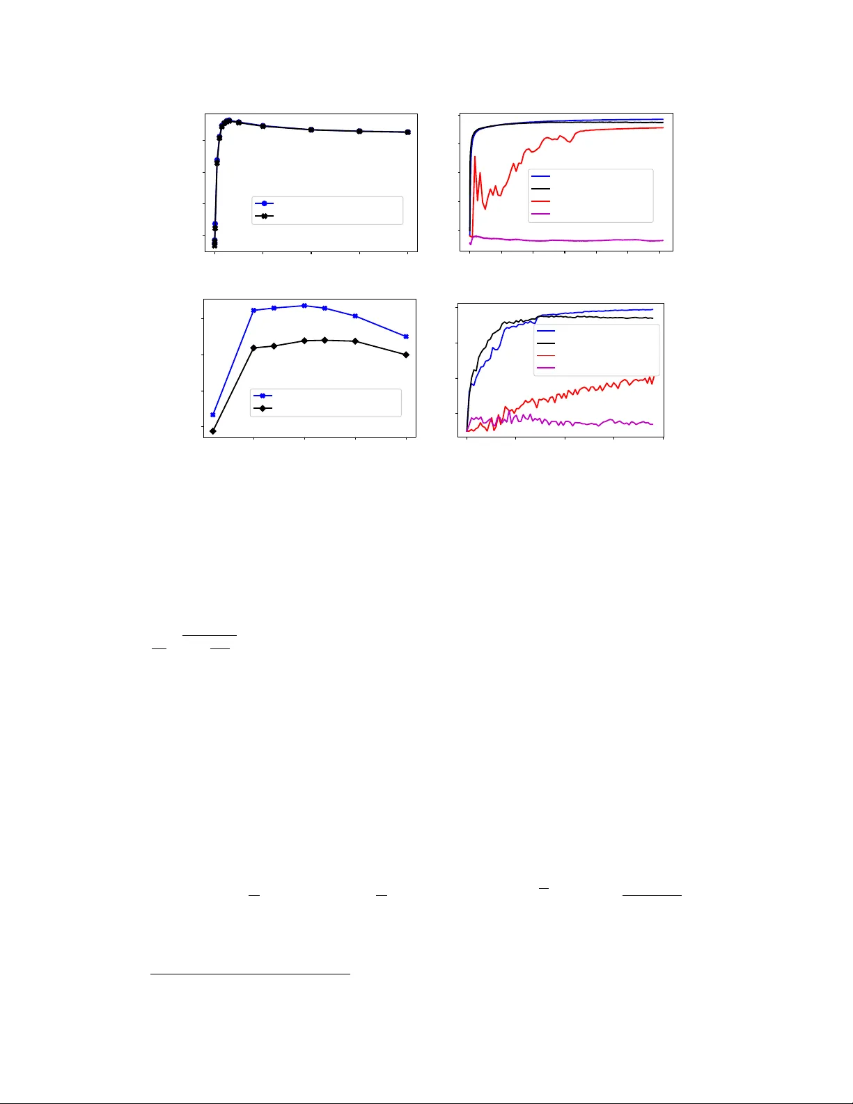
Stochastic-Sign SGD f or F ederated Lear ning with Theor etical Guarantees Richeng Jin ∗ , Y ufan Huang † , Xiaofan He ‡ , Huaiyu Dai § , Tianfu W u ¶ Abstract Federated learning (FL) has emerged as a prominent distributed learning paradigm. FL entails some pressing needs for dev eloping nov el parameter estimation ap- proaches with theoretical guarantees of con ver gence, which are also communication efﬁcient, dif ferentially priv ate and Byzantine resilient in the heterogeneous data distribution settings. Quantization-based SGD solvers hav e been widely adopted in FL and the recently proposed SIGN SGD with majority v ote shows a promising di- rection. Ho we ver , no existing methods enjoy all the aforementioned properties. In this paper , we propose an intuitiv ely-simple yet theoretically-sound method based on SIGN SGD to bridge the gap. W e present Stochastic-Sign SGD which utilizes nov el stochastic-sign based gradient compressors enabling the aforementioned properties in a uniﬁed framework. W e also present an error-feedback v ariant of the proposed Stochastic-Sign SGD which further improv es the learning performance in FL. W e test the proposed method with extensiv e experiments using deep neural networks on the MNIST dataset and the CIF AR-10 dataset. The experimental results corroborate the effecti veness of the proposed method. 1 Introduction Recently , Federated Learning (FL) has become a prominent distributed learning paradigm since it allows training on a large amount of decentralized data residing on de vices like mobile phones [1]. Howe ver , FL imposes se veral critical challenges. First of all, the communication capability of the mobile de vices can be a signiﬁcant bottleneck. Furthermore, the training data on a gi ven work er is typically based on its usage of the mobile de vices, which results in heterogeneous data distribution. In addition, the local data usually contains some sensitive information of a particular mobile de vice user . Therefore, there is an pressing need to develop a priv acy-preserving distrib uted learning algorithm. Finally , similar to many distributed learning methods, FL may suffer from malicious participants. As is sho wn in [2], ev en a single Byzantine worker , which may transmit arbitrary information, can sev erely disrupt the con ver gence of distributed gradient descent algorithms. Howe ver , to the best of our kno wledge, no existing methods can cope with all the aforementioned challenges. T o alleviate the communication burden of the w orkers, there hav e been various gradient quantization methods [3 – 7] in the literature, among which the recently proposed SIGN SGD with majority vote [8] is of particular interest due to its robustness and communication efﬁcienc y . 1 In SIGN SGD, during each communication round, only the signs of the gradients and aggregation results are exchanged between the workers and the server , which leads to around 32 × less communication than full-precision ∗ North Carolina State Univ ersity , Email: rjin2@ncsu.edu. † North Carolina State Univ ersity , Email: yhuang20@ncsu.edu. ‡ W uhan Univ ersity , Email: xiaofanhe@whu.edu.cn. § Corresponding author; North Carolina State Univ ersity , Email: hdai@ncsu.edu. ¶ North Carolina State Univ ersity , Email: tianfu wu@ncsu.edu. 1 Note that all the algorithms considered in this work use the idea of majority vote. Therefore, we ignore the term “with majority vote” in the follo wing discussions for the ease of presentation. Preprint. Under revie w . distributed SGD. Nonetheless, it has been shown in [9] that SIGN SGD fails to con ver ge when the data on different w orkers are heterogeneous (i.e., drawn from dif ferent distributions), which is one of the most important features in FL. In this work, inspired by the idea of adding carefully designed noise before taking the sign operation in [9], we present Stochastic-Sign SGD, which is a class of stochastic-sign based SGD algorithms. In particular , we ﬁrst propose a stochastic compressor sto - sig n , which extends SIGN SGD to its stochastic version Sto-SIGN SGD. In this scheme, instead of directly transmitting the signs of gradients, the work ers adopt a two-le vel stochastic quantization and transmit the signs of the quantized results. W e note that different from the existing 1-bit stochastic quantization schemes (e.g., QSGD [3], cpSGD [7]), the proposed algorithm also uses the majority vote rule in gradient aggregation, which allo ws the server - to-worker communication to be 1-bit compressed and ensures robustness as well. Then, to further resolve the priv acy concerns, a dif ferentially pri vate stochastic compressor dp - sig n is proposed, which can accommodate the requirement of ( , δ ) -local differential pri v acy [10]. The corresponding algorithm is termed as DP-SIGN SGD. W e then prove that both of the proposed algorithms conv erge to the neighborhood of the (local) optimum under heterogeneous data distribution. In addition, assuming that there are M normal (benign) workers, it is sho wn that the Byzantine resilience of the proposed algorithms is upper bounded by | P M m =1 ( g ( t ) m ) i | /b i , ∀ i , where ( g ( t ) m ) i is the i -th entry of worker m ’ s gradient at iteration t and b i ≥ max m ( g ( t ) m ) i is some design parameter . Particularly , b i depends on the data heterogeneity (through max m ( g ( t ) m ) i ). As a special case, the proposed algorithms can tolerate M − 1 Byzantine workers when the normal workers can access the same dataset (i.e., ( g ( t ) m ) i = ( g ( t ) j ) i , ∀ 1 ≤ j, m ≤ M ), which recov ers the result of SIGN SGD. W e also introduce weighted vote and T op- k sparsiﬁcation based schemes to improve resilience against attackers and differential pri v acy , respectively . Finally , we extend the proposed algorithm to its error-feedback v ariant, termed as Error -Feedback Stochastic-Sign SGD. In this scheme, the server keeps track of the error induced by the majority vote operation and compensates for the error in the next communication round. Both the con ver gence and the Byzantine resilience are established. Extensi ve simulations are performed to demonstrate the effecti veness of all the proposed algorithms. 2 Related W orks Gradient Quantization: T o accommodate the need of communication efﬁcienc y in distrib uted learning, various gradient compression methods hav e been proposed. Most of the existing works focus on unbiased methods [11, 12]. QSGD [3], T ernGrad [4] and A TOMO [13] propose to use stochastic quantization schemes, based on which a dif ferentially priv ate variant is proposed in [7]. Due to the unbiased nature of such quantization methods, the conv ergence of the corresponding algorithms can be established. The idea of sharing the signs of gradients in SGD can be traced back to 1-bit SGD [14]. Despite that sign-based quantization is biased in nature, [15] and [5, 8] show theoretical and empirical evidence that sign-based gradient schemes can con ver ge well in the homogeneous data distribution scenario. [16] shows that the con vergence of SIGN SGD can be guaranteed if the probability of wrong aggregation is less than 1 / 2 . In the heterogeneous data distribution case, [9] shows that the conv ergence of SIGN SGD is not guaranteed and proposes to add carefully designed noise to ensure a con ver gence rate of O ( d 3 4 /T 1 4 ) . Howe ver , their analysis assumes second order dif ferentiability of the noise probability density function and cannot be applied to some commonly used noise distributions (e.g., uniform and Laplace distributions). In addition, their analysis requires that the variance of the noise goes to inﬁnity as the number of iterations grows, which may be unrealistic in practice. [16] proposes Stochastic Sign Descent with Momentum (SSDM) to accommodate the data heterogeneity , and annother independent work proposes FedCOMGA TE [17]. Compared to SSDM and FedCOMGA TE, the proposed Stochastic-Sign SGD is stateless and therefore more suitable for cross-de vice FL [18]. Moreov er , the Byzantine resilience of Stochastic-Sign SGD is further quantiﬁed. Error -Compensated SGD: Instead of directly using the biased approximation of the gradients, [14] corrects the quantization error by adding error feedback in subsequent updates and observes almost no accuracy loss empirically . [6] proposes the error-compensated quantized SGD in quadratic optimization and proves its con ver gence for unbiased stochastic quantization. [19] proves the 2 con ver gence of the proposed error compensated algorithm for strongly-con vex loss functions and [20] prov es the con ver gence of sparsiﬁed gradient methods with error compensation for both conv ex and non-con ve x loss functions. In addition, [21] proposes EF-SIGN SGD, which combines the error compensation methods and SIGN SGD; ho wever , only the single worker scenario is considered. [22] further extends it to the multi-worker scenario and the conv ergence is established. Howe ver , it is required in these two works that the compressing error cannot be lar ger than the magnitude of the original vector , which is not the case for some biased compressors like SIGN SGD. [23] considers more general compressors and prov es the con vergence under the assumption that the compressors have bounded magnitude of error . Howe ver , to the best our kno wledge, none of the e xisting works consider the Byzantine resilience of the error-compensated methods. Byzantine T olerant SGD in Heterogenous En vironment: There hav e been signiﬁcant research interests in de veloping SGD based Byzantine tolerant algorithms, most of which consider homoge- neous data distribution, e.g., Krum [24], ByzantineSGD [25], and the median based algorithms [26]. [8] shows that SIGN SGD can tolerate up to half “blind” Byzantine workers who determine how to manipulate their gradients before observing the gradients. T o accommodate the need for robust FL, some Byzantine tolerant algorithms that can deal with heterogeneous data distributions ha ve been dev eloped. [27] proposes to incorporate a regularized term with the objectiv e function. Howe ver , it requires strong con ve xity and can only conv erge to the neighborhood of the optimal solution. [28] uses trimmed mean to aggre gate the shared parameters. [29] adopts the RA GE algorithm in [30] for robust aggre gation. Despite that these methods provide certain Byzantine resilience, none of them take the communication ef ﬁciency into consideration. Our Contributions. This paper makes three main contributions to the ﬁeld of FL as follo ws. 1. W e deriv e a sufﬁcient condition for the con ver gence of sign-based gradient descent meth- ods in the presence of data heterogeneity , based on which we propose the framework of Stochastic-Sign SGD, which utilizes the stochastic-sign based gradient compressors to ov ercome the con vergence issue of SIGN SGD gi ven heterogeneous data distribution. In particular , two nov el stochastic compressors, sto - sig n and dp - sig n , are proposed, which extend SIGN SGD to Sto-SIGN SGD and DP-SIGN SGD, respecti vely . DP-SIGN SGD is shown to improv e the priv acy and the accurac y simultaneously , without sacriﬁcing any communica- tion ef ﬁciency . W e further improve the learning performance of the proposed algorithm by incorporating the error-feedback method. 2. W e prov e that Sto-SIGN SGD conv erges to the neighborhood of the (local) optimum in the heterogeneous data distribution scenario. As the number of workers increases, the gap between the con ver ged solution and the (local) optimum decreases. 3. W e theoretically quantify the Byzantine resilience of the proposed algorithm, which depends on the heterogeneity of the local datasets of the workers. T o further improve the Byzantine resilience of Sto-SIGN SGD, a reputation based weighted vote mechanism is proposed and its effecti veness is v alidated by simulations. 3 Problem F ormulation In this paper , we consider a typical federated optimization problem with M normal workers as in [1]. Formally , the goal is to minimize the ﬁnite-sum objectiv e of the form min w ∈ R d F ( w ) where F ( w ) def = 1 M M X m =1 f m ( w ) . (1) For a machine learning problem, we have a sample space I = X × Y , where X is a space of feature vectors and Y is a label space. Giv en the hypothesis space W ⊆ R d , we deﬁne a loss function l : W × I → R which measures the loss of prediction on the data point ( x, y ) ∈ I made with the hypothesis vector w ∈ W . In such a case, f m ( w ) is a local function deﬁned by the local dataset of worker m and the hypothesis w . More speciﬁcally , f m ( w ) = 1 | D m | X ( x n ,y n ) ∈ D m l ( w ; ( x n , y n )) , (2) where | D m | is the size of work er m ’ s local dataset D m . If the training data are distrib uted over the workers uniformly at random, then we would hav e E [ f m ( w )] = F ( w ) , where the expectation is over 3 the training data distribution. This is the homogeneous data distribution assumption typically made in distributed optimization [1]. In many FL applications, ho wev er , the local datasets of the workers are heterogeneously distributed. W e consider a parameter server paradigm. At each communication round t , each worker m forms a batch of training samples, based on which it computes and transmits the stochastic gradient g ( t ) m as an estimate to the true gradient ∇ f m ( w ( t ) m ) . When the worker m ev aluates the gradient o ver its whole local dataset, we hav e g ( t ) m = ∇ f m ( w ( t ) m ) . After receiving the gradients from the work ers, the server performs aggregation and sends the aggre gated gradient back to the workers. Finally , the workers update their local model weights using the aggre gated gradient. In this sense, the classic stochastic gradient descent (SGD) algorithm [31] performs iterations of the form w ( t +1) m = w ( t ) m − η M M X m =1 g ( t ) m . (3) In this case, since all the workers adopt the same update rule using the aggregated gradient, w ( t ) m ’ s are the same for all the w orkers. Therefore, in the following discussions, we omit the worker index m for the ease of presentation. T o accommodate the requirement of communication ef ﬁciency in FL, we adopt the popular idea of gradient quantization and assume that each worker m quantizes the gradient with a stochastic 1-bit compressor q ( · ) and sends q ( g ( t ) m ) instead of its actual local gradient g ( t ) m . Combining with the idea of majority vote in [5], the corresponding algorithm is presented in Algorithm 1. Algorithm 1 Stochastic-Sign SGD with majority vote Input : learning rate η , current hypothesis vector w ( t ) , M workers each with an independent gradient g ( t ) m , the 1-bit compressor q ( · ) . on server: pull q ( g ( t ) m ) from work er m . push ˜ g ( t ) = sig n  1 M P M m =1 q ( g ( t ) m )  to all the workers. on each worker: update w ( t +1) = w ( t ) − η ˜ g ( t ) . Intuiti vely , the performance of Algorithm 1 is limited by the probability of wrong aggregation, which is giv en by sig n  1 M M X m =1 q ( g ( t ) m )  6 = sig n  1 M M X m =1 ∇ f m ( w ( t ) )  . (4) In SIGN SGD, q ( g ( t ) m ) = sig n ( g ( t ) m ) and (4) holds when ∇ f m ( w ( t ) ) 6 = ∇ f j ( w ( t ) ) , ∀ m 6 = j with a high probability , which prev ents its con v ergence. In this w ork, we propose two compressors sto - sig n and dp - sig n , which guarantee that (4) holds with a probability that is strictly smaller than 0.5 and therefore the con ver gence of Algorithm 1 follo ws. Moreover , dp - sig n is dif ferentially priv ate, i.e., giv en the quantized gradient q ( g ( t ) m ) , the adversary cannot distinguish the local dataset of w orker m from its neighboring datasets that differ in only one data point with a high probability . The detailed deﬁnition of differential pri v acy can be found in Section 1 of the supplementary document. In addition to the M normal workers, it is assumed that there exist B Byzantine attackers, and its set is denoted as B . Instead of using sto - sig n and dp - sig n , the Byzantine attackers can use an arbitrary compressor denoted by by z antine - sig n . In this work, we consider the scenario that the Byzantine attackers ha ve access to the average gradients of all the M normal workers (i.e., g ( t ) j = 1 M P M m =1 g ( t ) m , ∀ j ∈ B ) and follow the same procedure as the normal workers. Therefore, we assume that the Byzantine attacker j shares the opposite signs of the true gradients, i.e., by z antine - sig n ( g ( t ) j ) = − sig n ( g ( t ) j ) . In order to facilitate the con vergence analysis, the following commonly adopted assumptions are made. 4 Assumption 1. (Lower bound). F or all w and some constant F ∗ , we have objective value F ( w ) ≥ F ∗ . Assumption 2. (Smoothness). ∀ w 1 , w 2 , we r equir e for some non-ne gative constant L F ( w 1 ) ≤ F ( w 2 )+ < ∇ F ( w 2 ) , w 1 − w 2 > + L 2 || w 1 − w 2 || 2 2 , (5) wher e < · , · > is the standard inner pr oduct. Assumption 3. (V ariance bound). F or any worker m , the stochastic gradient oracle gives an independent unbiased estimate g m that has coor dinate bounded variance: E [ g m ] = ∇ f m ( w ) , E [(( g m ) i − ∇ f m ( w ) i ) 2 ] ≤ σ 2 i , (6) for a vector of non-ne gative constants ¯ σ = [ σ 1 , · · · , σ d ] ; ( g m ) i and ∇ f m ( w ) i ar e the i -th coor dinate of the stochastic and the true gr adient, respectively . Assumption 4. The total number of workers is odd. W e note that Assumptions 1, 2 and 3 are standard for non-con vex optimization and Assumption 4 is just to ensure that there is always a winner in the majority v ote [9], which can be easily relaxed. Experimental Settings. T o facilitate empirical discussions on our proposed algorithms in the remaining sections, we ﬁrst introduce our e xperimental settings here. W e implement our proposed method with a two-layer fully connected neural network on the standard MNIST dataset and VGG-9 [32] on the CIF AR-10 dataset. For MNIST , we use a ﬁxed learning rate, which is tuned from the set { 1 , 0 . 1 , 0 . 01 , 0 . 005 , 0 . 003 , 0 . 001 , 0 . 0001 } . For CIF AR-10, we tune the initial learning rate from the set { 1 , 0 . 1 , 0 . 01 , 0 . 001 , 0 . 0001 } , which is reduced by a factor of 2, 5, 10 and 20 at iteration 1,500, 3,000, 5,000 and 7,000, respecti vely . W e consider a scenario of M = 31 normal w orkers. T o simulate the heterogeneous data distrib ution scenario, each worker only stores e xclusiv e data for one out of the ten categories, unless otherwise noted. Besides, for MNIST , the w orkers ev aluate their gradients ov er the whole local datasets during each communication round, while for CIF AR-10, the w orkers train their local models with a mini-batch size of 32. More details about the implementation can be found in the supplementary document. 4 Algorithms and Con ver gence Analysis In this section, we ﬁrst derive a sufﬁcient condition for the con v ergence of sign-based gradient descent method in the presence of data heterogeneity . For the ease of presentation, we ﬁrst consider a scalar case, which can be readily generalized to the vector case by applying the results independently on each coordinate. Theorem 1. Let u 1 , u 2 , · · · , u M be M known and ﬁxed r eal numbers and consider binary r andom variables ˆ u m , 1 ≤ m ≤ M . Suppose that ¯ p = 1 M P M m =1 Pr  sig n  1 M P M m =1 u m  6 = ˆ u m  < 1 2 , we have P  sig n  1 M M X m =1 ˆ u m  6 = sig n  1 M M X m =1 u m  ≤  4 ¯ p (1 − ¯ p )  M 2 , (7) Remark 1. Let u m = ∇ f m ( w ( t ) ) i be the i -th coordinate of worker m ’ s true local gradient and ˆ u m = sig n ( g ( t ) m ) i the i -th coor dinate of the 1-bit estimator ,  4 ¯ p (1 − ¯ p )  M 2 < 1 / 2 is a suﬁcient condition that the pr obability of wr ong aggr e gation on the i -th coor dinate is less than 1 / 2 , where ¯ p = 1 M P M m =1 Pr( sig n ( 1 M P M m =1 ∇ f m ( w ( t ) ) i ) 6 = sig n ( g ( t ) m ) i ) char acterizes the impact of data heter ogeneity . Essentially , as long as ¯ p < 1 / 2 , there exists some M such that the pr obability of wr ong aggr e gation is less than 1 / 2 , and the con ver gence of the sign-based gradient descent method can be established. W e note that our work is differ ent fr om [16] in thr ee aspects: (1) we do not assume the same pr obability of wr ong signs Pr( sig n ( ∇ f m ( w ( t ) ) i ) 6 = sig n ( g ( t ) m ) i ) acr oss the workers; (2) instead of Pr( sig n ( ∇ f m ( w ( t ) ) i ) 6 = sig n ( g ( t ) m ) i ) < 1 / 2 , ∀ m , we only r equir e the averag e pr obability of wr ong signs ¯ p < 1 / 2 . (3) we propose a stoc hastic-sign based compr essor to over come the non-conver g ence issue of SIGN SGD when ¯ p ≥ 1 / 2 . W e emphasize that such a result is crucial in the heter og eneous data distribution scenario since the pr obability of wr ong signs can be very dif fer ent in this case. 5 In the above discussion, we sho w that SIGN SGD works for a sufﬁciently large M giv en that the av erage probability of wrong signs ¯ p < 1 / 2 . In the scenarios with more severe data heterogeneity where ¯ p ≥ 1 / 2 , howe ver , its conv ergence is not guaranteed. In the following, we propose two compressors sto - sig n and dp - sig n for the Stochastic-Sign SGD frame work, which can deal with the heterogeneous data distribution scenario. The basic ideas of the two compressors are giv en as follows. • sto - sig n : instead of directly sharing the signs of the gradients, sto - sig n ﬁrst performs a two-le vel stochastic quantization and then transmits the signs of the quantized results. • dp - sig n : it is a differentially priv ate v ersion of sto - sig n . The probability of each coordinate of the gradients mapping to {− 1 , 1 } is designed to accommodate the local differential priv acy requirements. 4.1 The Stochastic Compressor sto - sign Formally , the compressor sto - sig n is deﬁned as follows. Deﬁnition 1. F or any given gradient g ( t ) m , the compr essor sto - sig n outputs sto - sig n ( g ( t ) m , b ) , wher e b is a vector of design parameters. The i -th entry of sto - sig n ( g ( t ) m , b ) is given by sto - sig n ( g ( t ) m , b ) i =    1 , with pr obability b i +( g ( t ) m ) i 2 b i , − 1 , with pr obability b i − ( g ( t ) m ) i 2 b i , (8) wher e ( g ( t ) m ) i and b i ≥ max m | ( g ( t ) m ) i | ar e the i -th entry of g ( t ) m and b , r espectively . When q ( g ( t ) m ) = sig n ( g ( t ) m ) , the magnitude information of g ( t ) m is not utilized. As a result, ¯ p < 1 / 2 is not guaranteed. In the proposed compressor sto - sig n , the magnitude information is encoded in the mapping probabilities in (8). By introducing the stochasticity , sto - sig n essentially makes use of the magnitude information (without incurring additional communication ov erhead) such that the probability of wrong aggregation can be theoretically bounded for an arbitrary realization of g ( t ) m ’ s. Corollary 1. Let u 1 , u 2 , · · · , u M be M known and ﬁxed real numbers and consider bi- nary random variables ˆ u m = sto - sign ( u m , b ) , 1 ≤ m ≤ M . W e have ¯ p sto = 1 M P M m =1 Pr  sig n  1 M P M m =1 u m  6 = ˆ u m  = bM −| P M m =1 u m | 2 bM , and P  sig n  1 M M X m =1 ˆ u m  6 = sig n  1 M M X m =1 u m  ≤  1 − x 2  M 2 , (9) wher e x = | P M m =1 u m | bM . Remark 2. ( selection of b ) Accor ding to Cor ollary 1, the average probability of wr ong signs ¯ p sto < 1 2 is guaranteed when | P M m u m | > 0 , which ther efor e addr esses the non-con ver gence issue of SIGN SGD. Some discussions on the choice of the vector b in (8) ar e in or der . W e take the i -th entry of b as an example . In the FL application, the i -th entry of the gradient g ( t ) m corr esponds to u m in Cor ollary 1. Accor ding to the deﬁnition of sto - sig n , b i ≥ max m | ( g ( t ) m ) i | and 0 ≤ x = | P M m =1 ( g ( t ) m ) i | / ( b i M ) ≤ 1 . On the other hand,  1 − x 2  in (9) is a decr easing function of x (and therefor e an increasing function of b i ) when 0 ≤ x ≤ 1 . In this sense, once the requir ement b i ≥ max m | ( g ( t ) m ) i | is satisﬁed, the pr obability of wr ong aggr e gation can be bounded by (9), which becomes the tightest when the equality holds. Ther efor e, to minimize the pr obability of wr ong aggr e gation, the best strate gy is to select b i = max m | ( g ( t ) m ) i | . In practice, since max m | ( g ( t ) m ) i | is unknown, the selection of an appr opriate b is an inter esting pr oblem deserving further in vestigation. In our experiments, we examine the performance of sto - sig n with a ﬁxed vector b . Since the true gradients c hange during the tr aining pr ocess, it is possible that b i < max m | ( g ( t ) m ) i | for some i . In such cases, the pr obabilities deﬁned in (8) may fall out of the range [0 , 1] . W e r ound them to 1 if they ar e positive and 0 otherwise. 6 For the con vergence analysis, we ﬁrst consider the scenario in which all the workers are benign. The Byzantine resilience of sto - sig n and dp - sig n will be discussed in Section 5. In addition, we assume that each worker ev aluates the gradients over its whole local dataset for simplicity (i.e., g ( t ) m = ∇ f m ( w ( t ) ) , ∀ 1 ≤ m ≤ M ). Particularly , in federated learning, the workers usually compute ∇ f m ( w ( t ) ) due to the small size of the local dataset. The discussion about stochastic gradients is presented in Section 8. The proofs of the theoretical results are provided in Section 2 of the supplementary document. Theorem 2. Suppose Assumptions 1, 2 and 4 ar e satisﬁed, and the learning rate is set as η = 1 √ T d . Then by running Algorithm 1 with q ( g ( t ) m ) = sto - sig n ( ∇ f m ( w ( t ) ) , b ) (termed as Sto-SIGN SGD) for T iterations, we have 1 T T X t =1 ||∇ F ( w ( t ) ) || 1 ≤ 1 c  E [ F ( w (0) ) − F ( w ( T +1) )] √ d √ T + L √ d 2 √ T + 2 T T X t =1 d X i =1 |∇ F ( w ( t ) ) i | 1 p ( t ) i > 1 − c 2  ≤ 1 c  ( F ( w (0) ) − F ∗ ) √ d √ T + L √ d 2 √ T + 2 d X i =1 b i ∆( M )  , (10) wher e 0 < c < 1 is some positive constant, p ( t ) i is the pr obability that the ag gre gation on the i -coor dinate of the gradient is wr ong during the t -th communication r ound, and ∆( M ) is the solution to  1 − x 2  M 2 = 1 − c 2 . The second inequality is due to the fact that p ( t ) i > 1 − c 2 only if |∇ F ( w ( t ) ) i | b i ≤ ∆( M ) . Giv en the results in Theorem 1, the proof of Theorem 2 follo ws the well known strate gy of relating the norm of the gradient to the expected improv ement of the global objective in a single iteration. Then accumulating the improv ement over the iterations yields the con v ergence rate of the algorithm. Remark 3. Similar to SIGN SGD, the con verg ence rate of Sto-SIGN SGD depends on the L 1 -norm of the gradient. A detailed discussion on this featur e can be found in [5]. Note that compar ed to the con verg ence rate of SIGN SGD, there are two differ ences: the positive coef ﬁcient c < 1 and the gap term 2 P d i =1 b i ∆( M ) . It can be veriﬁed that ∆( M ) is a decr easing function of M and lim M →∞ ∆( M ) = 0 for any c < 1 , which suggests that the conver gence rate of Sto-SIGN SGD in the heter ogeneous data distribution scenario appr oaches that of SIGN SGD with homogeneous data distribution as the number of work ers incr eases. W e note that the last term in (10) captures the gap induced by the scenarios where the probability of wrong aggregation is lar ger than 1 − c i 2 , which vanishes as M grows to inﬁnity . One possible concern is that, gi ven a ﬁnite M , this term may be unbounded for lar ge b i ’ s. In the following, we introduce two scenarios where this term can be eliminated gi ven ﬁnite M . 4.1.1 Scenario 1: Large enough b i ’ s Essentially , the follo wing theorem can be prov ed in this case. Theorem 3. Given Assumption 4 and the same { u m } M m =1 and { ˆ u m } M m =1 as those in Theor em 1, we have P  sig n  1 M M X m =1 ˆ u m  6 = sig n  1 M M X m =1 u m  = 1 2 −  M − 1 M − 1 2  2 M b     M X m =1 u m     + O  1 b 2  . (11) According to Theorem 3, the probability of wrong aggregation is strictly smaller than 1 2 when | P M m =1 u m | > 0 and b is sufﬁciently lar ge such that the second term in (11) dominates. That being said, there always exists a positi ve constant c such that the probability of wrong aggregation is no larger than 1 − c 2 , and therefore the last term in (10) can be eliminated. In particular, if we select b i = T 1 / 4 d 1 / 4 , the following theorem can be pro ved. Theorem 4. Suppose Assumptions 1, 2 and 4 ar e satisﬁed, |∇ F ( w ( t ) ) i | ≤ Q, ∀ 1 ≤ i ≤ d, 1 ≤ t ≤ T , and the learning rate is set as η = 1 √ T d . Then by running Algorithm 1 with q ( g ( t ) m ) = 7 sto - sig n ( ∇ f m ( w ( t ) ) , b ) and b i = T 1 / 4 d 1 / 4 , ∀ i for T iterations, we have 1 T T X t =1 d X i =1 |∇ F ( w ( t ) ) i | 2 ≤ 2 M 2 M  M − 1 M − 1 2   ( F ( w (0) ) − F ∗ ) d 3 / 4 T 1 / 4 + Ld 3 / 4 2 T 1 / 4 + 2 T T X t =1 d X i =1 |∇ F ( w ( t ) ) i | O  1 T 1 / 4 d 1 / 4  ≤ √ 2 π ( M − 1) 3 2 2( M 2 − 3 M )  ( F ( w (0) ) − F ∗ ) d 3 / 4 T 1 / 4 + Ld 3 / 4 2 T 1 / 4 + 2 T T X t =1 d X i =1 |∇ F ( w ( t ) ) i | O  1 T 1 / 4 d 1 / 4  , (12) which further captur es the impact of M (i.e., √ 2 π ( M − 1) 3 2 2( M 2 − 3 M ) ≤ O ( 1 √ M ) ) compar ed to [9]. 4.1.2 Scenario 2: Bounded gradient dissimilarity W e note that Theorem 2 does not require any assumptions on the data heterogeneity across the clients. As a result, it is possible that |∇ F ( w ( t ) ) i | b i ≤ |∇ F ( w ( t ) ) i | max m |∇ f m ( w ( t ) ) | ≤ ∆( M ) as |∇ F ( w ( t ) ) i | decreases in the training process, which may lead to p ( t ) i > 1 − c 2 giv en the bound in (7). With such consideration, we can lo wer bound |∇ F ( w ( t ) ) i | max m |∇ f m ( w ( t ) ) | with the following coordinate-wise bounded gradient dissimilarity assumption. Assumption 5. (Bounded Gradient Dissimilarity) |∇ f m ( w ) i | ≤ B |∇ F ( w ) i | , ∀ w ∈ R d , 1 ≤ i ≤ d, m ∈ [1 , M ] . (13) Let b i = max m |∇ f m ( w ) i | , we hav e P  sig n  1 M M X m =1 sto - sig n ( g ( t ) m , b )  i 6 = sig n  1 M M X m =1 g ( t ) m  i  ≤  1 − 1 B 2  M 2 . (14) In this case, for any large enough M such that  1 − 1 B 2  M 2 < 1 2 , we can ﬁnd the corresponding c such that  1 − 1 B 2  M 2 = 1 − c 2 and the last term in (10) is eliminated. Remark 4. W e note that Assumption 5 can be understood as a strong er coor dinate-wise ver- sion of the local dissimilarity assumption in [33] which assumes that 1 M P M m =1 ||∇ f m ( w ) || 2 ≤ B 2 ||∇ F ( w ) || 2 , ∀ w . Experimental r esults. W e perform e xperiments to e xamine the learning performance of Sto-SIGN SGD for different selection of b . Throughout our experiments, in the ﬁxed b scenarios, we set b = b · 1 for some positive constant b . For “Optimal b ”, we set b i = max m | ( g ( t ) m ) i | , ∀ i . The results are shown in Figure 1. It can be observed that for ﬁxed b , b ﬁrst should be large enough to optimize the performance. Then, as b keeps increasing, both the training accuracy and the testing accuracy decrease, which corroborates our analysis above. Furthermore, for a gi ven total communication ov erhead, Sto-SIGN SGD with a ﬁxed b achiev es a higher testing accuracy than FedA vg (especially when the allowed communication overhead is small) and SIGN SGD and approaches that with the optimal b , which demonstrates its effecti veness. 4.2 The Differentially Pri vate Compressor dp - sign In this subsection, we present the dif ferentially priv ate version of sto - sig n . Formally , the compressor dp - sig n is deﬁned as follows. Deﬁnition 2. F or any given gr adient g ( t ) m , the compr essor dp - sig n outputs dp - sig n ( g ( t ) m , , δ ) . The i -th entry of dp - sig n ( g ( t ) m , , δ ) is given by dp - sig n ( g ( t ) m , , δ ) i =    1 , with pr obability Φ  ( g ( t ) m ) i σ  − 1 , with pr obability 1 − Φ  ( g ( t ) m ) i σ  (15) 8 0 . 0 0 . 1 0 . 2 0 . 3 0 . 4 b 0 . 2 0 . 4 0 . 6 0 . 8 Accuracy Sto-SIGNSGD-T raining Accuracy Sto-SIGNSGD-T esting Accuracy 0 5 10 15 20 25 30 Communication Overhead (MB) 0 . 2 0 . 4 0 . 6 0 . 8 1 . 0 T esting Accuracy Sto-SIGNSGD-Optimal b Sto-SIGNSGD- b = 0 . 03 FedAvg 5-Lo cal Iterations SIGNSGD 0 . 005 0 . 010 0 . 015 0 . 020 b 0 . 5 0 . 6 0 . 7 0 . 8 Accuracy Sto-SIGNSGD-T raining Accuracy Sto-SIGNSGD-T esting Accuracy 0 1000 2000 3000 4000 Communication Overhead (MB) 0 . 2 0 . 4 0 . 6 0 . 8 T esting Accuracy Sto-SIGNSGD-Optimal b Sto-SIGNSGD- b = 0 . 01 FedAvg-10 Lo cal Iterations SIGNSGD Figure 1: The two ﬁgures in the ﬁrst and the second ro ws sho w the performance of Sto-SIGN SGD on MNIST and CIF AR-10, respectively . All the presented results are averaged o ver 5 repeats. The ﬁrst column shows the training and the testing accuracy of Sto-SIGN SGD for different b = b · 1 . W e run 200 and 8,000 communication rounds for MNIST and CIF AR-10, respectiv ely . The second column compares the testing accuracy of Sto-SIGN SGD with SIGN SGD and FedA vg [1] with respect to the total communication ov erhead. FedA vg uses a learning rate decay of 0.99 and 0.996 per communication round for MNIST and CIF AR-10, respectiv ely . W e tune the number of local iterations from the set { 1, 5, 10, 20 } and present the results with the best ﬁnal testing accuracy . wher e Φ( · ) is the cumulative distribution function of the normalized Gaussian distribution; σ = ∆ 2  q 2 ln( 1 . 25 δ ) , where  and δ ar e the differ ential privacy parameter s and ∆ 2 is the sensitivity measur e. 2 Theorem 5. The pr oposed compr essor dp - sig n ( · , , δ ) is ( , δ ) -differ entially private for any , δ ∈ (0 , 1) . Remark 5. Note that thr oughout this paper , we assume δ > 0 . F or the δ = 0 scenario, the Laplace mechanism [10] can be used by r eplacing the cumulative distribution function of the normalized Gaussian distribution in (15) with that of the Laplace distrib ution. The corr esponding discussion is pr ovided in the supplementary document. W e term Algorithm 1 with q ( g ( t ) m ) = dp - sig n ( g ( t ) m , , δ ) as DP-SIGN SGD. Similar to sto - sig n , we consider the scalar case and obtain the following result for dp - sig n ( · , , δ ) . Theorem 6. Let u 1 , u 2 , · · · , u M be M known and ﬁxed real numbers. Further deﬁne r andom variables ˆ u i = dp - sig n ( u i , , δ ) , ∀ 1 ≤ i ≤ M . Then ther e always e xist a constant σ 0 such that when σ ≥ σ 0 , P ( sig n ( 1 M P M m =1 ˆ u i ) 6 = sig n ( 1 M P M m =1 u i )) <  1 − x 2  M 2 , wher e x = | P M m =1 u m | 2 σ M . Giv en Theorem 6, the conv ergence of DP-SIGN SGD can be obtained by following a similar analysis to that of Theorem 2. 2 Please refer to Section 1 of the supplementary document for detailed information about the differential priv acy parameters (  , δ ) and the sensitivity measure ∆ 2 . 9 5 Byzantine Resilience In this section, the Byzantine resilience of the sign-based gradient descent method is in vestigated. W e note that the conv ergence of Algorithm 1 is limited by the probability of wrong aggregation (i.e., more than half of the workers share the wrong signs). In the following analysis, we as- sume that the Byzantine attackers ev aluate their gradients ov er the whole training dataset, i.e., by z antine - sig n ( g ( t ) j ) = − sig n ( ∇ F ( w ( t ) )) , ∀ j ∈ B , which is considered the worst case sce- nario . The study can be easily e xtended to other scenarios when the Byzantine attackers are more constrained in their capabilities. Let Z i denote the number of normal workers that share (quan- tized) gradients with different signs from the true gradient ∇ F ( w ( t ) ) on the i -th coordinate (i.e., q ( g ( t ) m ) i 6 = sig n ( ∇ F ( w ( t ) ) i ) ). Then, Z i is a Poisson binomial variable. In order to tolerate k i Byzantine workers that alw ays share the wrong signs on the i -th coordinate of the gradient, we need to hav e P ( Z i ≥ M − k i 2 ) ≤ 1 − c 2 for some positiv e constant c , where M is the number of benign workers. Therefore, we can prove the follo wing theorem. Theorem 7. During t -th communication r ound, let 1 M P M m =1 Pr  sig n  ∇ F ( w ( t ) )  i 6 = q ( g ( t ) m ) i  = ¯ p ( t ) i , then Algorithm 1 can at least tolerate k i Byzantine attacker s on the i -th coor dinate of the gr adient and k i satisﬁes 1. ¯ p ( t ) i ≤ M − k i 2 M . 2. Ther e exists some positive constant c such that " ( M − k i )(1 − ¯ p ( t ) i ) ( M + k i ) ¯ p ( t ) i # k 2 r M − k i M + k i + r M + k i M − k i ! M × h ¯ p ( t ) i (1 − ¯ p ( t ) i ) i M 2 ≤ 1 − c 2 . (16) Overall, the number of Byzantine worker s that the algorithms can tolerate is given by min 1 ≤ i ≤ d k i . Remark 6. When q ( g ( t ) m ) = sto - sig n ( ∇ f m ( w ( t ) ) , b ) , we have ¯ p ( t ) i = b i M −| P M m =1 ∇ f m ( w ( t ) ) i | 2 b i M and the ﬁrst condition in Theor em 7 is reduced to k i ≤ | P M m =1 ∇ f m ( w ( t ) ) i | b i . In this sense , if we set b i = max m |∇ f m ( w ( t ) ) i | as in Section 4, the ﬁrst condition in Theorem 7 gives k i < | P M m =1 ∇ f m ( w ( t ) ) i | max m |∇ f m ( w ( t ) ) i | , which means that the Byzantine resilience depends on the heter ogene- ity of the local datasets. In an ideal scenario wher e the workers have the same local datasets, 3 i.e., ∇ f m ( w ( t ) ) i = ∇ f n ( w ( t ) ) i , ∀ m, n , Theor em 7 gives ¯ p ( t ) i = 0 and k i < M . Ther efor e, it can tolerate M − 1 Byzantine worker s. Remark 7. Our analysis of the con ver gence and the Byzantine r esilience is based on each individual coor dinate of the gr adients, which corr esponds to the dimensional Byzantine resilience [34]. Further- mor e, for a ﬁxed b , the gradients (and ther efor e the Byzantine resilience) tend to decr ease during the training pr ocess. W ith such consideration, we pr opose a r eputation based weighted vote mechanism to impr ove the Byzantine resilience , which can be found in Section 6. Mor e speciﬁcally , the server can identify the normal worker s in the be ginning of the training pr ocess with higher pr obabilities and assign higher weights to them in majority vote. Experimental r esults. Fig. 2 shows the performance of Sto-SIGN SGD for different selection of b = b · 1 and different number of Byzantine workers B . It can be seen that as the number of Byzantine workers increases, both the training and the testing accuracy of Sto-SIGN SGD with a larger b drop much faster than that with a smaller b , which conforms to our analysis above that a lager b results in worse Byzantine resilience. It is also observed that SIGN SGD essentially fails in this extremely heterogeneous data distribution setting (where each worker holds exclusiv e data), ev en without attackers. Furthermore, to examine the impact of data heterogeneity , we vary the number of labels of each worker’ s local training dataset in T able 1. It can be observed that the testing accuracy of SIGN SGD im- prov es when the training data become more homogeneously distributed across workers. Furthermore, 3 W e note that this can be relaxed for weaker attackers that do not ha ve access to the whole training dataset. 10 0 1 2 3 Number of Byzantine work ers B 0 . 0 0 . 2 0 . 4 0 . 6 0 . 8 T esting Accuracy Optimal b b = 0 . 03 b = 0 . 1 b = 0 . 2 SIGNSGD 0 1 2 3 Number of Byzantine wo rkers B 0 . 2 0 . 4 0 . 6 0 . 8 T esting Accuracy Optimal b b = 0 . 015 b = 0 . 01 b = 0 . 005 SIGN SGD Figure 2: The left and right ﬁgures show the testing accuracy of Sto-SIGN SGD for different number of Byzantine workers and dif ferent b on MNIST and CIF AR-10, respectiv ely . For MNIST , the Byzantine workers ev aluate their gradients ov er the whole training dataset. For CIF AR-10, each Byzantine worker has 2,000 training examples that are sampled from the training dataset uniformly at random. The mini-batch sizes of all the workers and the Byzantine attack ers are set to 32. T able 1: T esting Accuracy of Sto-SIGN SGD on MNIST B S I G N S G D 2 L A B E L S O P T I M A L b 2 L A B E L S S I G N S G D 4 L A B E L S O P T I M A L b 4 L A B E L S 0 7 0 . 0 3 % 9 2 . 3 4 % 9 0 . 5 3 % 9 3 . 1 2 % 1 6 6 . 3 1 % 9 3 . 1 4 % 8 8 . 2 1 % 9 3 . 3 8 % 2 6 0 . 1 9 % 9 2 . 7 1 % 8 7 . 3 4 % 9 3 . 3 9 % 3 5 6 . 2 3 % 9 1 . 1 3 % 8 2 . 4 9 % 9 2 . 1 9 % 4 4 7 . 4 4 % 8 4 . 4 9 % 8 1 . 5 1 % 9 2 . 3 1 % both SIGN SGD and Sto-SIGN SGD obtain better Byzantine resilience as the number of labels increases. Finally , Sto-SIGN SGD with optimal b still outperforms SIGN SGD, which indicates that introducing the stochasticity is still beneﬁcial in the more homogeneous data distribution scenarios. 6 Impro ved Resilience with W eighted V ote According to Theorem 7, it is shown that the number of Byzantine attackers that Sto-SIGN SGD can tolerate decreases as the gradient | P M m =1 ∇ f m ( w ( t ) ) | decreases. As a result, Sto-SIGN SGD is more robust against Byzantine attack ers in the beginning of the training process. W ith such consideration, a reputation based weighted vote mechanism is proposed and the corresponding algorithm is presented in Algorithm 2. In the proposed mechanism, the server stores a credit r ( t ) m for each worker . During each iteration, gi ven the shared signs of the gradients from the workers, the server ﬁrst performs a weighted vote gi ven by (17). Then, the aggregated result ˜ g ( t ) is used as the “ground truth”, based on which a credit is assigned to each worker . More speciﬁcally , in (18), P d i =1 1 ˜ g ( t ) i = q ( g ( t ) m ) i /d and P d i =1 1 ˜ g ( t ) i 6 = q ( g ( t ) m ) i /d measures the number of coordinates that w orker m shares the same and different signs compared to the aggregated result, respectiv ely . Considering that in the beginning of the training process, the probability of correct aggregation is high, and the attackers that deliberately share wrong signs are expected to receiv e lower credits and therefore play a smaller role in the future iterations. As a result, the impact of the attackers is reduced. Experimental results. Fig. 3 sho ws the performance of Sto-SIGN SGD with weighted v ote. It can be observed that for MNIST , Sto-SIGN SGD with weighted vote obtains a comparable testing accuracy in the presence of up to 3 Byzantine workers compared to Sto-SIGN SGD without Byzantine workers. For CIF AR-10, it can be observed that Sto-SIGN SGD div erges in the presence of 5 Byzantine attackers. In the meantime, Sto-SIGN SGD with weighted vote achieves almost the same testing accuracy against 5 Byzantine workers as Sto-SIGN SGD without Byzantine workers. Furthermore, Sto-SIGN SGD with weighted vote achieves a higher testing accuracy against 10 Byzantine workers compared to Sto- SIGN SGD against 1 Byzantine worker , which v alidates its ef fectiv eness. 11 Algorithm 2 Stochastic-Sign SGD with weighted vote Input : learning rate η , current hypothesis vector w ( t ) , M workers each with an independent gradient g ( t ) m , the 1-bit compressor q ( · ) , initialized credit r (0) m = 1 , ∀ m . on server: pull q ( g ( t ) m ) from work er m and compute the weighted vote giv en by ˜ g ( t ) = sig n  1 M M X m =1 max { r ( t ) m , 0 } q ( g ( t ) m )  (17) push ˜ g ( t ) to all the workers and update the credits r ( t +1) m = r ( t ) m + P d i =1 [ 1 ˜ g ( t ) i = q ( g ( t ) m ) i − 1 ˜ g ( t ) i 6 = q ( g ( t ) m ) i ] d , (18) where ˜ g ( t ) i and q ( g ( t ) m ) i are the i -th entry of the aggregated result ˜ g ( t ) and the v ector q ( g ( t ) m ) shared by worker m , respecti vely . on each worker: update w ( t +1) = w ( t ) − η ˜ g ( t ) . 0 1 2 3 Number of Byzantine wo rkers B 0 . 0 0 . 2 0 . 4 0 . 6 0 . 8 T esting Accuracy Algorithm 2, b = 0 . 03 Algorithm 1, Optimal b Algorithm 1, b = 0 . 03 SIGNSGD 0 2000 400 0 6000 800 0 Communication Rounds 0 . 2 0 . 4 0 . 6 T esting Accuracy 0 attacker w/o weighted vote 1 attacker w/o weighted vote 5 attacker w/o weighted vote 5 attackers with weighted vote 10 attackers with weighted vote SIGNSGD-0 attacker Figure 3: The left ﬁgure shows the testing accurac y of Sto-SIGN SGD with weighted v ote on MNIST with b = 0 . 03 · 1 and dif ferent number of Byzantine workers that ev aluate their gradients ov er the whole training dataset. The right ﬁgure shows the testing accuracy of Sto-SIGN SGD with weighted vote on CIF AR-10, with b = 0 . 012 · 1 . Each Byzantine worker has 2,000 training examples that are sampled from the training dataset uniformly at random. The mini-batch sizes of all the workers and the Byzantine attackers are set to 32. 7 Impro ved Differential Pri vacy with Sparsiﬁcation Intuitiv ely , according to Theorem 6, as the absolute value of the true gradient |∇ F ( w ( t ) ) i | decreases, the corresponding probability of wrong aggregation increases. In this sense, discarding the coordinates with higher probabilities of wrong aggregation may help improve the learning performance. Therefore, we propose to improve the performance of DP-SIGN SGD by incorporating the T op-K sparsiﬁcation scheme [35, 36]. The corresponding algorithm is termed as DP-T opSIGN SGD and presented in Algorithm 3. Experimental results. W e compare our proposed dif ferentially priv ate scheme with DP-Fed SGD [37], a direct extension of DP- SGD [38] to the distrib uted setting, where differential priv acy is provided through additi ve Gaussian noise. Moreover , we further incorporate the T op-K sparsiﬁcation scheme [35, 36] into DP-SIGN SGD. In this case, each client only sends 10% of the coordinates of the gradients with the largest magnitudes through the dp - sig n compressor , and the corresponding algorithm is termed as DP-T opSIGN SGD. The corresponding results are presented in Fig. 4, where we run the algorithms for 200 communication rounds and utilize the notion of Gaussian differential priv acy for priv acy composition [39]. W e set σ ∈ { 10 , 20 , 30 , 50 , 80 } , which provide µ -Gaussian differential priv acy guarantees of µ ∈ { 5 . 66 , 2 . 83 , 1 . 89 , 1 . 13 , 0 . 71 } ; in terms of common notion 12 Algorithm 3 DP-SIGN SGD with sparsiﬁcation Input : learning rate η , current hypothesis vector w ( t ) , M workers each with an independent gradient g ( t ) m , the 1-bit compressor q ( · ) , the T op- k sparsiﬁer top k ( · ) . on server: pull dp - sig n ( top k ( g ( t ) m )) from work er m . push ˜ g ( t ) = sig n  1 M P M m =1 dp - sig n ( top k ( g ( t ) m ))  to all the workers. on each worker: update w ( t +1) = w ( t ) − η ˜ g ( t ) . 20 40 60 80 σ 0 . 6 0 . 7 0 . 8 T esting Accuracy MNIST DP-Fed SGD DP-SIGN SGD DP-T opSIGN SGD Figure 4: Performance of DP-T opSIGN SGD, DP-SIGN SGD and DP-Fed SGD on MNIST . W e follow the idea of gradient clipping in [38] to bound the sensiti vity ∆ 2 . After computing the gradient for each individual training sample in the local dataset, each worker clips it in its L 2 norm for a clipping threshold C to ensure that ∆ 2 ≤ C . W e set C = 4 in the experiments. of differential priv acy , this corresponds to  ∈ { 4 . 05 , 1 . 48 , 0 . 83 , 0 . 38 , 0 . 18 } for the commonly considered δ = 10 − 5 . 4 It can be seen that DP-SIGN SGD performs similarly with DP-Fed SGD for the same le vel of priv acy protection, while enjoying an improv ement of 32 × in communication efﬁcienc y . DP-T opSIGN SGD outperforms DP-Fed SGD and the improvement increases as σ increases (which indicates more stringent requirement for pri vac y), while further reduces the communication ov erhead (compared to DP-SIGN SGD). 8 Extending to SGD Up until this point in the paper, the discussions are based on the assumption that each worker can e valuate its local true gradient ∇ f m ( w ( t ) ) for the ease of presentation. In the SGD scenario, we hav e to further account for the sampling noise. Particularly , the following theorem for Sto-SIGN SGD can be prov ed. The corresponding result for DP-SIGN SGD can be obtained following a similar strategy . Theorem 8. Suppose Assumptions 1-4 are satisﬁed, and set the learning rate η = 1 √ T d . Then, when b = b · 1 and b is sufﬁciently lar ge, Sto-SIGN SGD conver g es to the (local) optimum if either of the following two conditions is satisﬁed. • P  sig n ( 1 M P M m =1 ( g t m ) i ) 6 = sig n ( ∇ F ( w t ) i  < 0 . 5 , ∀ 1 ≤ i ≤ d . • The mini-batch size of stochastic gr adient at each iteration is at least T . Remark 8. Note that the ﬁrst condition is not hard to satisfy . One sufﬁcient condition is that the sampling noise of each worker is symmetric with zer o mean. This assumption is also used in [8], which shows that the sampling noise is appr oximately not only symmetric, b ut also unimodal. Remark 9. W e note that the above discussion assumes that b is sufﬁciently lar ge , which guarantees that the probability of wr ong aggr e gation is less than 0.5. F or an arbitrary b that satisﬁes the condition in the deﬁnition of sto - sig n , we believe that it is possible to pr ove that the algorithm con ver ges to the neighborhood of the (local) optimum. In particular , similar to the pr oof of Theor em 4 Essentially , a mechanism is µ -Gaussian differential pri v acy if and only if it is ( , δ (  )) -differential pri vac y with δ (  ) = Φ( −  µ + µ 2 ) − e  Φ( −  µ − µ 2 ) . 13 2, ther e will be an additional term P d i =1 |∇ F ( w t ) i | 1 | 1 M P M m =1 ( g t m ) i |≤ b ∆( M ) . It is possible to upper bound this additional term given the fact that E [ 1 M P M m =1 ( g t m ) i ] = ∇ F ( w t ) i , despite that more efforts ar e r equir ed to make the analysis rigor ous. 9 Extending to Error -feedback V ariant T o further improved the performance of Algorithm 1, we incorporate the error -feedback technique and propose its error-feedback v ariant (i.e., Algorithm 4), where the server utilizes an α -approximate compressor C ( · ) (i.e., ||C ( x ) − x || 2 2 ≤ (1 − α ) || x || 2 2 , ∀ x [21]) and keeps track of the corresponding compression error . Algorithm 4 Error-Feedback Stochastic-Sign SGD with majority v ote Input : learning rate η , current hypothesis vector w ( t ) , current residual error vector ˜ e ( t ) , M workers each with an independent gradient g ( t ) m = ∇ f m ( w ( t ) ) , the 1-bit compressor q ( · ) . on server: pull q ( g ( t ) m ) from work er m . push ˜ g ( t ) = C  1 M P M m =1 q ( g ( t ) m ) + ˜ e ( t )  to all the workers, update residual err or: ˜ e ( t +1) = 1 M M X m =1 q ( g ( t ) m ) + ˜ e ( t ) − ˜ g ( t ) . (19) on each worker: update w ( t +1) = w ( t ) − η ˜ g ( t ) . Remark 10. Note that in Algorithm 4, only the server adopts the err or-feedback method. When dp - sig n is used, implementing err or-feedbac k on the worker’ s side may incr ease the privacy leakage. Accounting for the additional privacy leakage caused by err or -feedback is left as futur e work. Both sto - sig n and dp - sig n can be used in Algorithm 4 and the corresponding algorithms are termed as EF-Sto-SIGN SGD and EF-DP-SIGN SGD, respecti vely . In the follo wing, we show the conv ergence and Byzantine resilience of Algorithm 4 when sto - sig n is used. The results can be easily adapted for dp - sig n . Particularly , the following theorems can be prov ed. Theorem 9. When Assumptions 1, 2 and 4 ar e satisﬁed, by running Algorithm 4 with η = 1 √ T d , q ( g ( t ) m ) = sto - sig n ( ∇ f m ( w ( t ) ) , b ) and b = b · 1 , we have 1 T T − 1 X t =0 ||∇ F ( w ( t ) ) || 2 2 b ≤ ( F ( w 0 ) − F ∗ ) √ d √ T + (1 + L + L 2 β ) √ d √ T , (20) wher e β is some positive constant. Remark 11. Theor em 9 shows that if b i ’ s ar e upper bounded (i.e ., when |∇ f m ( w ( t ) ) i | ≤ Q, ∀ m, t, i as in [9]), EF-Sto-SIGN SGD can con ver ge to the (local) optimum while Sto-SIGN SGD only con ver ges to the neighborhood of optimum (c.f. Theorem 2). In our experiments, the server adopts the compr essor C ( x ) = 1 M sig n ( x ) . In this case, the communi- cation overhead of EF-Sto-SIGN SGD is essentially the same as Sto-SIGN SGD. Utilizing the fact that the output of the compr essor q ( · ) ∈ {− 1 , 1 } , it can be r eadily shown that || 1 M sig n ( x ) − x || 2 2 < || x || 2 2 with x = 1 M P M m =1 q ( g ( t ) m ) + ˜ e ( t ) , which suggests that ther e exists some α such that C ( · ) is α - appr oximate compr essor . More details can be found in Section 4 of the supplementary document. Besides the fact that error-feedback is only used on the server’ s side, another difference between Algorithm 4 and those in [21, 22] is that it does not require the workers to share the magnitude information about the gradients. On the one hand, it sav es communication ov erhead. On the other hand, it keeps the resilience against the re-scaling attacks. By following a similar strategy to the proofs of Theorem 9 and considering the impact of Byzantine attackers, we obtain the Byzantine resilience of Algorithm 4 as follows. 14 0.0 0.2 0.4 0.6 0.8 ε 0.2 0.4 0.6 0.8 T esting Accuracy DP-SIGNSGD-T esting Accuracy EF-DP-SIGNSGD-T esting Accuracy 0 50 100 15 0 200 Communication Rounds 0 . 2 0 . 4 0 . 6 0 . 8 T esting Accuracy Sto-SIGNSGD-No Attacker Sto-SIGNSGD-1 Attacker EF-Sto-SIGNSGD-No Attacker EF-Sto-SIGNSGD-1 Attacker 0 2000 4000 6000 8000 Communication Rounds 0 . 2 0 . 4 0 . 6 0 . 8 T esting Accuracy Sto-SIGNSGD-No Attacker Sto-SIGNSGD-3 Attackers EF-Sto-SIGNSGD-No Attacker EF-Sto-SIGNSGD-3 Attackers Figure 5: The ﬁrst ﬁgure shows the performance of DP-SIGN SGD and EF-DP-SIGN SGD on MNIST for different  when δ = 10 − 5 , without Byzantine attackers. The  ’ s measure the per epoch priv acy guarantee of the algorithms. The second ﬁgure compares Sto-SIGN SGD with EF-Sto-SIGN SGD on MNIST with b = 0 . 02 · 1 . The last ﬁgure compares Sto-SIGN SGD with EF-Sto-SIGN SGD on CIF AR-10 with optimal b . Theorem 10. At each iteration t , Algorithm 4 can at least tolerate k i = | P M m =1 ∇ f m ( w ( t ) ) i | /b Byzantine attack ers on the i -th coor dinate of the gradient. Overall, the number of Byzantine workers that Algorithm 4 can tolerate is given by min 1 ≤ i ≤ d k i . Experimental results. For DP-SIGN SGD and EF-DP-SIGN SGD, we follo w the idea of gradient clipping in [38] to bound the sensitivity ∆ 2 . After computing the gradient for each individual training sample in the local dataset, each worker clips it in its L 2 norm for a clipping threshold C to ensure that ∆ 2 ≤ C . W e set C = 4 in the experiments and the results are shown in the ﬁrst ﬁgure of Fig. 5. It can be observed that when there is no Byzantine attackers, EF-DP-SIGN SGD outperforms DP-SIGN SGD for all the examined  ’ s, which demonstrates its effecti veness. Another observ ation is that the error -feedback v ariants do not necessarily perform better . For instance, in the last ﬁgure of Fig. 5, when there are 3 Byzantine attackers, the testing accurac y of EF-Sto-SIGN SGD is worse than that of Sto-SIGN SGD. In the beginning of the training process, k i ’ s in Theorem 10 are large enough such that the algorithm can tolerate the Byzantine attacker . As the gradients decrease, the probability of wrong aggregation increases. In this case, the error-feedback mechanism may carry the wrong aggregations to the future iterations and ha ve a ne gativ e impact on the learning process. 10 Conclusion W e propose a Stochastic-Sign SGD frame work which utilizes two no vel gradient compressors and can deal with heterogeneous data distribution. The proposed algorithms are proved to con ver ge in the heterogeneous data distribution scenario with the same rate as SIGN SGD in the homogeneous data distribution case. In particular , the proposed differentially pri vate compressor dp - sig n improv es the priv acy and the accurac y simultaneously without sacriﬁcing any communication ef ﬁciency . Then, we further impro ve the learning performance of the proposed method by incorporating the error-feedback scheme. In addition, the Byzantine resilience of the proposed algorithms is sho wn analytically . It is expected that the proposed algorithms can ﬁnd wide applications in the design of communication efﬁcient, dif ferentially pri vate and Byzantine resilient FL algorithms. 15 Supplementary Material The supplementary material is organized as follo ws. In Section 1, we formally provide the deﬁnition of local differential priv acy [10]. In Section 2, we provide the proofs of the theoretical results presented in the main document. Discussions about the extended dif ferentially pri vate compressor dp - sig n when δ = 0 are provided in Section 3. Discussions about the server’ s compressor C ( · ) in Algorithm 4 are provided in Section 4. The details about the implementation of our experiments and some additional experimental results are presented in Section 5. 1 Deﬁnition of Local Differential Pri vacy In this work, we study the pri vacy guarantee of the proposed algorithms from the lens of local differential priv acy [10], which provides a strong notion of individual pri vac y in data analysis. The deﬁnition of local differential pri v acy is formally gi ven as follo ws. Deﬁnition 3. Given a set of local datasets D pr ovided with a notion of neighboring local datasets N D ⊂ D × D that differ in only one data point. F or a query function f : D → X , a mechanism M : X → O to r elease the answer of the query is deﬁned to be ( , δ ) -locally differ entially private if for any measurable subset S ⊆ O and two neighboring local datasets ( D 1 , D 2 ) ∈ N D , P ( M ( f ( D 1 )) ∈ S ) ≤ e  P ( M ( f ( D 2 )) ∈ S ) + δ. (21) A key quantity in characterizing local dif ferential pri vac y for many mechanisms is the sensitivity of the query f in a given norm l r , which is deﬁned as ∆ r = max ( D 1 ,D 2 ) ∈N D || f ( D 1 ) − f ( D 2 ) || r . (22) For more details about the concept of dif ferential priv acy , the reader is referred to [10] for a survey . 2 Proofs 2.1 Proof of Theor em 1 Theorem 1. Let u 1 , u 2 , · · · , u M be M known and ﬁxed r eal numbers and consider binary r andom variables ˆ u m , 1 ≤ m ≤ M . Suppose that ¯ p = 1 M P M m =1 Pr  sig n  1 M P M m =1 u m  6 = ˆ u m  < 1 2 , we have P  sig n  1 M M X m =1 ˆ u m  6 = sig n  1 M M X m =1 u m  ≤  4 ¯ p (1 − ¯ p )  M 2 , (23) Pr oof. Deﬁne a series of random variables { X m } M m =1 giv en by X m =        1 , if ˆ u m 6 = sig n  1 M P M m =1 u m  , − 1 , if ˆ u m = sig n  1 M P M m =1 u m  . (24) In particular , X m can be considered as the outcome of one Bernoulli trial with successful probability P ( X m = 1) , and we hav e P  sig n  1 M M X m =1 ˆ u m  6 = sig n  1 M M X m =1 u m  = P M X m =1 X m ≥ 0 ! . (25) For an y variable a > 0 , we have P M X m =1 X m ≥ 0 ! = P  e a P M m =1 X m ≥ e 0  ≤ E [ e a P M m =1 X m ] e 0 = E [ e a P M m =1 X m ] , (26) 16 which is due to Markov’ s inequality , gi ven the fact that e a P M m =1 X m is non-negati ve. For the ease of presentation, let P ( X m = 1) = p m , we hav e, E [ e a P M m =1 X m ] = e ln( E [ e a P M m =1 X m ]) = e ln( Q M m =1 E [ e aX m ]) = e P M m =1 ln( E [ e aX m ]) = e P M m =1 ln( e a p m + e − a (1 − p m )) = e M ( 1 M P M m =1 ln( e a p m + e − a (1 − p m )) ) ≤ e M ln( e a ¯ p + e − a (1 − ¯ p )) , (27) where ¯ p = 1 M P M m =1 p m and the inequality is due to Jensen’ s inequality . Optimizing a yields a = ln  q 1 − ¯ p ¯ p  > 0 and e M ln( e a ¯ p + e − a (1 − ¯ p )) = [4 ¯ p (1 − ¯ p )] M 2 , (28) which completes the proof. 2.2 Proof of Cor ollary 1 Corollary 1. Let u 1 , u 2 , · · · , u M be M known and ﬁxed real numbers and consider bi- nary random variables ˆ u m = sto - sig n ( u m , b ) , 1 ≤ m ≤ M . W e have ¯ p = 1 M P M m =1 Pr  sig n  1 M P M m =1 u m  6 = ˆ u m  = bM −| P M m =1 u m | 2 bM , and P  sig n  1 M M X m =1 ˆ u m  6 = sig n  1 M M X m =1 u m  ≤  1 − x 2  M 2 , (29) wher e x = | P M m =1 u m | bM . Pr oof. It can be easily shown that ¯ p = 1 M P M m =1 Pr  sig n  1 M P M m =1 u m  6 = ˆ u m  = bM −| P M m =1 u m | 2 bM when ˆ u m = sto - sig n ( u m , b ) . Plugging it into (23) completes the proof. 2.3 Proof of Theor em 2 Theorem 2. Suppose Assumptions 1, 2 and 4 are satisﬁed, and the learning r ate is set as η = 1 √ T d . Then by running Sto-SIGN SGD for T iterations, we have 1 T T X t =1 ||∇ F ( w ( t ) ) || 1 ≤ 1 c  E [ F ( w (0) ) − F ( w ( T +1) )] √ d √ T + L √ d 2 √ T + 2 η T T X t =1 d X i =1 |∇ F ( w ( t ) ) i | 1 p ( t ) i > 1 − c 2  ≤ 1 c  ( F ( w (0) ) − F ∗ ) √ d √ T + L √ d 2 √ T + 2 d X i =1 b i ∆( M )  , (30) wher e 0 < c < 1 is some positive constant, p ( t ) i is the pr obability that the ag gre gation on the i -coor dinate of the gradient is wr ong during the t -th communication r ound, and ∆( M ) is the solution to  1 − x 2  M 2 = 1 − c 2 . The second inequality is due to the fact that p ( t ) i > 1 − c 2 only if |∇ F ( w ( t ) ) i | b i ≤ ∆( M ) . The proof of Theorem 2 follows the well known strategy of relating the norm of the gradient to the expected improvement of the global objective in a single iteration. Then accumulating the improv ement over the iterations yields the con v ergence rate of the algorithm. 17 Pr oof. According to Assumption 2, we have F ( w ( t +1) ) − F ( w ( t ) ) ≤ < ∇ F ( w ( t ) ) , w ( t +1) − w ( t ) > + L 2 || w ( t +1) − w ( t ) || 2 = − η < ∇ F ( w ( t ) ) , sig n  1 M M X m =1 sto - sig n ( g ( t ) m )  > + L 2         η sig n  1 M M X m =1 sto - sig n ( g ( t ) m )          2 = − η < ∇ F ( w ( t ) ) , sig n  1 M M X m =1 sto - sig n ( g ( t ) m )  > + Lη 2 d 2 = − η ||∇ F ( w ( t ) ) || 1 + Lη 2 d 2 + 2 η d X i =1 |∇ F ( w ( t ) ) i | 1 sig n ( 1 M P M m =1 sto - sig n ( g ( t ) m ) i ) 6 = sig n ( ∇ F ( w ( t ) ) i ) , (31) where ∇ F ( w ( t ) ) i is the i -th entry of the vector ∇ F ( w ( t ) ) and η is the learning rate. T aking expectation on both sides yeilds E [ F ( w ( t +1) ) − F ( w ( t ) )] ≤ − η ||∇ F ( w ( t ) ) || 1 + Lη 2 d 2 + 2 η d X i =1 |∇ F ( w ( t ) ) i | P  sig n  1 M M X m =1 sto - sig n ( g ( t ) m ) i  6 = sig n ( ∇ F ( w ( t ) ) i )  (32) Let ∆( M ) denote the solution to  1 − x  e x  M 2 = 1 − c 2 . Since  1 − x  e x is a decreasing function of x for 0 < x < 1 , it can be veriﬁed that  1 − x  e x  M 2 < 1 − c 2 when x > ∆( M ) and  1 − x  e x  M 2 ≥ 1 − c 2 otherwise. According to Theorem 1, we hav e two possible scenarios as follows. P  sig n  1 M M X m =1 sto - sig n ( g ( t ) m ) i  6 = sig n ( ∇ F ( w ( t ) ) i )     ≤ 1 − c 2 , if |∇ F ( w ( t ) ) i | b i > ∆( M ) , ≤ 1 , if |∇ F ( w ( t ) ) i | b i ≤ ∆( M ) . (33) Plugging (33) into (32), we can obtain E [ F ( w ( t +1) ) − F ( w ( t ) )] ≤ − η ||∇ F ( w ( t ) ) || 1 + Lη 2 d 2 + η  (1 − c ) d X i =1 |∇ F ( w ( t ) ) i | 1 p ( t ) i ≤ 1 − c 2 + (1 − c ) d X i =1 |∇ F ( w ( t ) ) i | 1 p ( t ) i > 1 − c 2  + 2 η d X i =1 |∇ F ( w ( t ) ) i | 1 p ( t ) i > 1 − c 2 ≤ − η ||∇ F ( w ( t ) ) || 1 + Lη 2 d 2 + η (1 − c ) ||∇ F ( w ( t ) ) || 1 + 2 η d X i =1 |∇ F ( w ( t ) ) i | 1 p ( t ) i > 1 − c 2 = − η c ||∇ F ( w ( t ) ) || 1 + Lη 2 d 2 + 2 η d X i =1 |∇ F ( w ( t ) ) i | 1 p ( t ) i > 1 − c 2 , (34) where p ( t ) i = P  sig n  1 M P M m =1 sto - sig n ( g ( t ) m ) i  6 = sig n ( ∇ F ( w ( t ) ) i )  is the probability of wrong aggregation. Adjusting the above inequality and averaging both sides o ver t = 1 , 2 , · · · , T , we can 18 obtain 1 T T X t =1 η c ||∇ F ( w ( t ) ) || 1 ≤ E [ F ( w (0) ) − F ( w ( T +1) )] T + Lη 2 d 2 + 2 η T T X t =1 d X i =1 |∇ F ( w ( t ) ) i | 1 p ( t ) i > 1 − c 2 ≤ E [ F ( w (0) ) − F ( w ( T +1) )] T + Lη 2 d 2 + 2 η d X i =1 b i ∆( M ) , (35) where the last inequality is due to the fact that p ( t ) i > 1 − c 2 only when |∇ F ( w ( t ) ) i | b i ≤ ∆( M ) . Letting η = 1 √ dT and dividing both sides by cη gives 1 T T X t =1 ||∇ F ( w ( t ) ) || 1 ≤ 1 c  E [ F ( w (0) ) − F ( w ( T +1) )] √ d √ T + L √ d 2 √ T + 2 η T T X t =1 d X i =1 |∇ F ( w ( t ) ) i | 1 p ( t ) i > 1 − c 2  ≤ 1 c  ( F ( w (0) ) − F ∗ ) √ d √ T + L √ d 2 √ T + 2 d X i =1 b i ∆( M )  , (36) which completes the proof. 2.4 Proof of Theor em 3 Theorem 3. Given Assumption 3 and the same { u m } M m =1 and { ˆ u m } M m =1 as those in Theor em 1, we have P  sig n  1 M M X m =1 ˆ u m  6 = sig n  1 M M X m =1 u m  = 1 2 −  M − 1 M − 1 2  2 M b     M X m =1 u m     + O  1 b 2  (37) Pr oof. W ithout loss of generality , assume u 1 ≤ u 2 ≤ · · · ≤ u K < 0 ≤ u K +1 ≤ · · · ≤ u M . According to the deﬁnition of sto - sig n , we hav e ˆ u m = sto - sig n ( u m , b ) = ( 1 , with probability b + u m 2 b , − 1 , with probability b − u m 2 b , (38) Further deﬁne a series of random variables { ˆ X m } M m =1 giv en by ˆ X m = ( 1 , if ˆ u m = 1 , 0 , if ˆ u m = − 1 . (39) In particular , ˆ X m can be considered as the outcome of one Bernoulli trial with successful probability P ( ˆ X m = 1) . Let ˆ Z = P M m =1 ˆ X m , then P  sig n  1 M M X m =1 ˆ u m  = 1  = P  ˆ Z ≥ M 2  = M X H = M +1 2 P ( ˆ Z = H ) . (40) In addition, P ( ˆ Z = H ) = P A ∈ F H Q i ∈ A ( b + u i ) Q j ∈ A c ( b − u j ) (2 b ) M = a M ,H b M + a M − 1 ,H b M − 1 + · · · + a 0 ,H b 0 (2 b ) M , (41) in which F H is the set of all subsets of H integers that can be selected from { 1 , 2 , 3 , ..., M } ; a m,H , ∀ 0 ≤ m ≤ M is some constant. It can be easily veriﬁed that a M ,H =  M H  . 19 When b is suf ﬁciently large, P ( ˆ Z = H ) is dominated by the ﬁrst two terms in (41). As a result, we hav e P ( ˆ Z = H ) = a M ,H b M + a M − 1 ,H b M − 1 (2 b ) M + O  1 b 2  . (42) In particular , ∀ m , we hav e X A ∈ F H Y i ∈ A ( b + u i ) Y j ∈ A c ( b − u j ) = ( b + u m ) X A ∈ F H ,m ∈ A Y i ∈ A/ { m } ( b + u i ) Y j ∈ A c ( b − u j ) + ( b − u m ) X A ∈ F H ,m / ∈ A Y i ∈ A ( b + u i ) Y j ∈ A c / { m } ( b − u j ) . (43) As a result, when M +1 2 ≤ H ≤ M − 1 , the u m related term in a M − 1 ,H is giv en by  M − 1 H − 1  −  M − 1 H  u m . (44) When H = M , the u m related term in a M − 1 ,H is giv en by  M − 1 H − 1  u m . (45) By summing ov er m , we have a M − 1 ,H =  M − 1 H − 1  −  M − 1 H  M X m =1 u m , if M + 1 2 ≤ H ≤ M − 1 , (46) and a M − 1 ,H =  M − 1 H − 1  M X m =1 u m , if H = M . (47) By summing ov er H , we have M X H = M +1 2 a M ,H = M X H = M +1 2  M H  = 2 M − 1 , (48) M X H = M +1 2 a M − 1 ,H =  M − 1 M − 1 2  M X m =1 u m . (49) As a result, P  sig n  1 M M X m =1 ˆ u m  = 1  = P  ˆ Z ≥ M 2  = M X H = M +1 2 P ( ˆ Z = H ) = 2 M − 1 b M +  M − 1 M − 1 2  P M m =1 u m b M − 1 (2 b ) M + O  1 b 2  = 1 2 +  M − 1 M − 1 2  2 M b M X m =1 u m + O  1 b 2  . (50) Therefore, P  sig n  1 M M X m =1 ˆ u m  6 = sig n  1 M M X m =1 u m  = 1 2 −  M − 1 M − 1 2  2 M b     M X m =1 u m     + O  1 b 2  . (51) 20 2.5 Proof of Theor em 4 Theorem 4. Suppose Assumptions 1, 2 and 4 ar e satisﬁed, |∇ F ( w ( t ) ) i | ≤ Q, ∀ 1 ≤ i ≤ d, 1 ≤ t ≤ T , and the learning rate is set as η = 1 √ T d . Then by running Algorithm 1 with q ( g ( t ) m ) = sto - sig n ( ∇ f m ( w ( t ) ) , b ) and b i = T 1 / 4 d 1 / 4 , ∀ i for T iterations, we have 1 T T X t =1 d X i =1 |∇ F ( w ( t ) ) i | 2 ≤ 2 M 2 M  M − 1 M − 1 2   ( F ( w (0) ) − F ∗ ) d 3 / 4 T 1 / 4 + Ld 3 / 4 2 T 1 / 4 + 2 T T X t =1 d X i =1 |∇ F ( w ( t ) ) i | O  1 T 1 / 4 d 1 / 4  ≤ √ 2 π ( M − 1) 3 2 2( M 2 − 3 M )  ( F ( w (0) ) − F ∗ ) d 3 / 4 T 1 / 4 + Ld 3 / 4 2 T 1 / 4 + 2 T T X t =1 d X i =1 |∇ F ( w ( t ) ) i | O  1 T 1 / 4 d 1 / 4  , (52) which further captur es the impact of M (i.e., √ 2 π ( M − 1) 3 2 2( M 2 − 3 M ) ≤ O ( 1 √ M ) ) compar ed to [9]. Pr oof. According to (32), we have E [ F ( w ( t +1) ) − F ( w ( t ) )] ≤ − η ||∇ F ( w ( t ) ) || 1 + Lη 2 d 2 + 2 η d X i =1 |∇ F ( w ( t ) ) i | P  sig n  1 M M X m =1 sto - sig n ( g ( t ) m ) i  6 = sig n ( ∇ F ( w ( t ) ) i )  (53) According to Lemma 3 P  sig n  1 M M X m =1 sto - sig n ( g ( t ) m ) i  6 = sig n ( ∇ F ( w ( t ) ) i )  = 1 2 − M  M − 1 M − 1 2  2 M b i   ∇ F ( w ( t ) ) i   + O  1 b 2 i  (54) Plugging (33) into (53), we can obtain E [ F ( w ( t +1) ) − F ( w ( t ) )] ≤ − η ||∇ F ( w ( t ) ) || 1 + Lη 2 d 2 + 2 η d X i =1 |∇ F ( w ( t ) ) i |  1 2 − M  M − 1 M − 1 2  2 M b i   ∇ F ( w ( t ) ) i   + O  1 b 2 i  = Lη 2 d 2 − η 2 M  M − 1 M − 1 2  2 M d X i =1 |∇ F ( w ( t ) ) i | 2 b i + 2 η d X i =1 |∇ F ( w ( t ) ) i | O  1 b 2 i  (55) Rearranging (55) giv es η 2 M  M − 1 M − 1 2  2 M d X i =1 |∇ F ( w ( t ) ) i | 2 b i ≤ E [ F ( w ( t ) ) − F ( w ( t +1) )] + Lη 2 d 2 + 2 η d X i =1 |∇ F ( w ( t ) ) i | O  1 b 2 i  (56) Adjusting the abov e inequality and averaging both sides o ver t = 1 , 2 , · · · , T yields 1 T T X t =1 d X i =1 |∇ F ( w ( t ) ) i | 2 b i ≤ 2 M 2 M  M − 1 M − 1 2   ( F ( w (0) ) − F ∗ ) η + Ldη 2 + 2 T T X t =1 d X i =1 |∇ F ( w ( t ) ) i | O  1 b 2 i  . (57) 21 Setting η = 1 √ T d and b i = T 1 / 4 d 1 / 4 giv es 1 T T X t =1 d X i =1 |∇ F ( w ( t ) ) i | 2 ≤ 2 M 2 M  M − 1 M − 1 2   ( F ( w (0) ) − F ∗ ) d 3 / 4 T 1 / 4 + Ld 3 / 4 2 T 1 / 4 + 2 T T X t =1 d X i =1 |∇ F ( w ( t ) ) i | O  1 T 1 / 4 d 1 / 4  (58) It is known that n n +1 e − n √ 2 π √ n ≤ n ! < n n +1 e − n √ 2 π √ n − 1 [40]. W ith some algebra, we can show that 2 M 2 M ( M − 1 M − 1 2 ) < √ 2 π ( M − 1) 3 2 2( M 2 − 3 M ) ≤ O ( 1 √ M ) . Therefore, we hav e 1 T T X t =1 d X i =1 |∇ F ( w ( t ) ) i | 2 ≤ √ 2 π ( M − 1) 3 2 2( M 2 − 3 M )  ( F ( w (0) ) − F ∗ ) d 3 / 4 T 1 / 4 + Ld 3 / 4 2 T 1 / 4 + 2 T T X t =1 d X i =1 |∇ F ( w ( t ) ) i | O  1 T 1 / 4 d 1 / 4  (59) which completes the proof. 2.6 Proof of Theor em 5 Theorem 5. The pr oposed compr essor dp - sig n ( · , , δ ) is ( , δ ) -differ entially private for any , δ ∈ (0 , 1) . Pr oof. W e start from the one-dimension scenario and consider any a, b that satisfy || a − b || 2 ≤ ∆ 2 . W ithout loss of generality , assume that dp - sign ( a, , δ ) = dp - sig n ( b, , δ ) = 1 . Then we ha ve P ( dp - sig n ( a, , δ ) = 1) = Φ  a σ  = Z a −∞ 1 √ 2 π σ e − x 2 2 σ 2 dx, P ( dp - sig n ( b, , δ ) = 1) = Φ  b σ  = Z b −∞ 1 √ 2 π σ e − x 2 2 σ 2 dx. (60) Furthermore, P ( dp - sig n ( a, , δ ) = 1) P ( dp - sig n ( b, , δ ) = 1) = R a −∞ e − x 2 2 σ 2 dx R b −∞ e − x 2 2 σ 2 dx = R ∞ 0 e − ( x − a ) 2 2 σ 2 dx R ∞ 0 e − ( x − b ) 2 2 σ 2 dx . (61) According to Theorem A.1 in [10], given the parameters , δ and σ , it can be veriﬁed that e −  ≤   P ( dp - sign ( a,,δ )=1) P ( dp - sign ( b,,δ )=1)   ≤ e  with probability at least 1 − δ . For the multi-dimension scenario, consider any vector a and b such that || a − b || 2 ≤ ∆ 2 and v ∈ {− 1 , 1 } d , we hav e P ( dp - sig n ( a , , δ ) = v ) P ( dp - sig n ( b , , δ ) = v ) = R D e − || x − a || 2 2 2 σ 2 d x R D e − || x − b || 2 2 2 σ 2 d x , (62) where D is some integral area depending on v . Similarly , it can be shown that e −  ≤   P ( dp - sign ( a ,,δ )= v ) P ( dp - sign ( b ,,δ )= v )   ≤ e  with probability at least 1 − δ . 2.7 Proof of Theor em 6 Theorem 6. Let u 1 , u 2 , · · · , u M be M known and ﬁxed real numbers. Further deﬁne r andom variables ˆ u i = dp - sig n ( u i , , δ ) , ∀ 1 ≤ i ≤ M . Then ther e always e xist a constant σ 0 such that when σ ≥ σ 0 , P ( sig n ( 1 M P M m =1 ˆ u i ) 6 = sig n ( 1 M P M m =1 u i )) <  1 − x 2  M 2 , wher e x = | P M m =1 u m | 2 σ M . 22 The proof of Theorem 6 follo ws a similar strate gy to that of Theorem 1. The difﬁculty we need to ov ercome is that unlike sto - sig n , the expectation of the number of workers that share the wrong signs is not a function of 1 M P M m =1 u i due to the nonlinearity introduced by Φ( · ) . Howe ver , when σ is large enough, we sho w that it can be upper bounded as a function of 1 M P M m =1 u i . Pr oof. W ithout loss of generality , assume u 1 ≤ u 2 ≤ · · · ≤ u K < 0 ≤ u K +1 ≤ · · · ≤ u M and 1 M P M i =1 u i < 0 . Note that similar analysis can be done when 1 M P M i =1 u i > 0 . W e are interested in obtaining ¯ p dp = 1 M P M m =1 Pr  sig n  1 M P M m =1 u m  6 = ˆ u m  . In particular , Pr sig n 1 M M X m =1 u m ! 6 = ˆ u m ! = Φ  u m σ  , (63) ¯ p dp = 1 M M X m =1 Pr sig n 1 M M X m =1 u m ! 6 = ˆ u m ! = 1 M M X m =1 Φ  u m σ  . (64) Let n denote a zero-mean Gaussian noise with v ariance σ , according to the assumption that u 1 ≤ u 2 ≤ · · · ≤ u K < 0 ≤ u K +1 ≤ · · · ≤ u M , we hav e Φ  u m σ  = 1 2 − P ( u m < n < 0) , ∀ 1 ≤ m ≤ K , Φ  u m σ  = 1 2 + P (0 < n < u m ) , ∀ K + 1 ≤ m ≤ M . (65) Therefore, ¯ p dp = 1 M M X m =1 Φ  u m σ  = 1 2 − 1 M  K X m =1 P ( u m < n < 0) − M X m = K +1 P (0 < n < u m )  . (66) Note that for any Gaussian noise, P ( a 1 < n < 0) + P ( a 2 < n < 0) ≥ P ( a 1 + a 2 < n < 0) for any a 1 < 0 , a 2 < 0 . Therefore, we consider the worst case scenario such that P K m =1 P ( u m < n < 0) − P M m = K +1 P (0 < n     M X m =1 u m      1 √ 2 π σ e − u 2 1 2 σ 2  + P  − M X m =2 u m < n < 0  − M X m =2 P (0 < n     M X m =1 u m      1 √ 2 π σ e − u 2 1 2 σ 2  −     M X m =2 u m     1 √ 2 π σ  1 − e − ( P M m =2 u m ) 2 2 σ 2  = 1 √ 2 π σ      M X m =1 u m     e − u 2 1 2 σ 2 +     M X m =2 u m      e − ( P M m =2 u m ) 2 2 σ 2 − 1  , (67) where the ﬁrst inequality is due to f ( a ) > f ( u 1 ) for a ∈ ( u 1 , P M m =1 u m ] and the second inequality is due to f ( a ) < 1 √ 2 π σ for any a > 0 , where f ( · ) is the probability density function of the normal distribution. 23 In particular, as σ → ∞ , | P M m =1 u m | e − u 2 1 2 σ 2 increases and con verges to | P M m =1 u m | while | P M m =2 u m |  e − ( P M m =2 u m ) 2 2 σ 2 − 1  increases and con ver ges to 0. Therefore, we have 1 √ 2 π σ      M X m =1 u m     e − u 2 1 2 σ 2 +     M X m =2 u m      e − ( P M m =2 u m ) 2 2 σ 2 − 1  σ →∞ − − − − → − P M m =1 u m √ 2 π σ . (68) As a result, there exists a σ 0 such that when σ ≥ σ 0 , we hav e ¯ p dp = 1 M M X m =1 Φ  u m σ  ≤ 1 2 + P M m =1 u m 4 M σ . (69) Follo wing the same analysis as that in the proof of Corollary 1, we can show that P  sig n  1 M M X m =1 ˆ u i  6 = sig n  1 M M X m =1 u i  <  1 − x 2  M 2 , (70) where x = | P M m =1 u m | 2 σ M . 2.8 Proof of Theor em 7 Theorem 7. During t -th communication r ound, let 1 M P M m =1 Pr  sig n  ∇ F ( w ( t ) )  i 6 = q ( g ( t ) m ) i  = ¯ p ( t ) i , then Algorithm 1 can at least tolerate k i Byzantine attacker s on the i -th coor dinate of the gr adient and k i satisﬁes 1. ¯ p ( t ) i ≤ M − k i 2 M . 2. Ther e exists some positive constant c such that " ( M − k i )(1 − ¯ p ( t ) i ) ( M + k i ) ¯ p ( t ) i # k 2 r M − k i M + k i + r M + k i M − k i ! M h ¯ p ( t ) i (1 − ¯ p ( t ) i ) i M 2 ≤ 1 − c 2 . (71) Overall, the number of Byzantine worker s that the algorithms can tolerate is given by min 1 ≤ i ≤ d k i . W e ﬁrst provide some intuition about the proof. It has been shown in the proof of Theorem 2 that the con ver gence of Algorithm 1 is guaranteed if there e xists some positiv e constant c such that the probability of more than half of the w orkers sharing wrong signs is no lar ger than 1 − c 2 . On the i -th coordinate of the gradient, if there are k i Byzantine workers that alw ays share the wrong signs, then at most M − k i 2 normal workers can share wrong signs such that the aggre gated result is still correct. Pr oof. W e ﬁrst consider the same setting as in Theorem 1 and deﬁne a series of random variables { X m } M m =1 giv en by X m =        1 , if ˆ u m 6 = sig n  1 M P M m =1 u m  , − 1 , if ˆ u m = sig n  1 M P M m =1 u m  . (72) In addition, let { ˆ u j } M + k i j = M +1 denote the binary variables shared by the Byzantine attackers. Then, X m can be considered as the outcome of one Bernoulli trial with successful probability P ( X m = 1) , and we hav e P   sig n   1 M + k i   M X m =1 ˆ u m + k i X j = M +1 ˆ u j     6 = sig n 1 M M X m =1 u m !   = P M X m =1 X m + k i ≥ 0 ! . (73) 24 For an y variable a > 0 , we have P M X m =1 X m + k i ≥ 0 ! = P  e a ( P M m =1 X m + k i ) ≥ e 0  ≤ E [ e a ( P M m =1 X m + k i ) ] e 0 = E [ e a ( P M m =1 X m + k i ) ] , (74) which is due to Markov’ s inequality , given the fact that e a ( P M m =1 X m + k i ) is non-negati ve. For the ease of presentation, let P ( X m = 1) = p m , we hav e, E [ e a ( P M m =1 X m + k i ) ] = e ln( E [ e a ( P M m =1 X m + k i ) ]) = e ln( Q M m =1 E [ e aX m ])+ ak i = e P M m =1 ln( E [ e aX m ])+ ak i = e ak i + P M m =1 ln( e a p m + e − a (1 − p m )) = e ak i + M ( 1 M P M m =1 ln( e a p m + e − a (1 − p m )) ) ≤ e ak i + M ln( e a ¯ p + e − a (1 − ¯ p )) , (75) where ¯ p = 1 M P M m =1 p m and the inequality is due to Jensen’ s inequality . Optimizing a yields a = ln  q ( M − k i )(1 − ¯ p ) ( M + k i ) ¯ p  > 0 and e ak i + M ln( e a ¯ p + e − a (1 − ¯ p )) =  ( M − k i )(1 − ¯ p ) ( M + k i ) ¯ p  k 2 r M − k i M + k i + r M + k i M − k i ! M [ ¯ p (1 − ¯ p )] M 2 . (76) In addition, a = ln  q ( M − k i )(1 − ¯ p ) ( M + k i ) ¯ p  > 0 indicates ¯ p < M − k i 2 M . Setting sig n ( ∇ F ( w ( t ) )) i = sig n ( 1 M P M m =1 u M ) and ˆ u m = q ( g ( t ) m ) i completes the proof. 2.9 Proof of Theor em 8 Theorem 8. Suppose Assumptions 1-4 are satisﬁed, and set the learning rate η = 1 √ T d . Then, when b = b · 1 and b is sufﬁciently lar ge, Sto-SIGN SGD conver g es to the (local) optimum if either of the following two conditions is satisﬁed. • P  sig n ( 1 M P M m =1 ( g t m ) i ) 6 = sig n ( ∇ F ( w t ) i  < 0 . 5 , ∀ 1 ≤ i ≤ d . • The mini-batch size of stochastic gr adient at each iteration is at least T . Pr oof. Note that in the proof of Theorem 2 and Lemma 3, we obtain E [ F ( w ( t +1) ) − F ( w ( t ) )] ≤ − η ||∇ F ( w ( t ) ) || 1 + Lη 2 d 2 + 2 η d X i =1 |∇ F ( w ( t ) ) i | P  sig n  1 M M X m =1 q ( g ( t ) m ) i  6 = sig n  1 M M X m =1 ∇ f m ( w ( t ) ) i  , (77) and P  sig n  1 M M X m =1 q ( g ( t ) m ) i  6 = sig n  1 M M X m =1 ( g ( t ) m ) i  < 1 2 − M  M − 1 M − 1 2  2 M b i   1 M M X m =1 ( g ( t ) m ) i   + O  1 b 2 i  , (78) where q ( g ( t ) m ) = sto - sig n ( g ( t ) m ) in Sto-SIGN SGD. 25 W e ﬁrst prove the con v ergence under the ﬁrst condition. For the ease of notation, let p i, 1 = P  sig n  1 M M X m =1 q ( g ( t ) m ) i  6 = sig n  1 M M X m =1 ( g ( t ) m ) i  = 1 2 − M  M − 1 M − 1 2  2 M b i   1 M M X m =1 ( g ( t ) m ) i   + O  1 b 2 i  , p i, 2 = P  sig n  1 M M X m =1 ∇ f m ( w ( t ) ) i  6 = sig n  1 M M X m =1 ( g ( t ) m ) i  < 1 2 , p i = P  sig n  1 M M X m =1 q ( g ( t ) m ) i  6 = sig n  1 M M X m =1 ∇ f m ( w ( t ) ) i  . (79) Then p i = p i, 1 (1 − p i, 2 ) + p i, 2 (1 − p i, 1 ) = p i, 1 + p i, 2 − 2 p i, 1 p i, 2 = p i, 2 + (1 − 2 p i, 2 ) p i, 1 = p i, 2 + (1 − 2 p i, 2 )   1 2 − M  M − 1 M − 1 2  2 M b i   1 M M X m =1 ( g ( t ) m ) i   + O  1 b 2 i    = 1 2 − (1 − 2 p i, 2 )   M  M − 1 M − 1 2  2 M b i   1 M M X m =1 ( g ( t ) m ) i   − O  1 b 2 i    (80) Follo wing the same strategy as that in the proof of Theorem 4, the con vergence can be established as follows. 1 T T X t =1 d X i =1 |∇ F ( w ( t ) ) i | 2 ≤ √ 2 π ( M − 1) 3 2 2( M 2 − 3 M )  ( F ( w (0) ) − F ∗ ) d 3 / 4 T 1 / 4 (1 − 2 p i, 2 ) + Ld 3 / 4 2 T 1 / 4 (1 − 2 p i, 2 ) + 2 T T X t =1 d X i =1 |∇ F ( w ( t ) ) i | O  1 T 1 / 4 d 1 / 4  (81) Then, we prove the con vergence under the second condition. According to (80), it is obvious that p i ≤ p i, 1 + p i, 2 . Therefore, we hav e d X i =1 |∇ F ( w ( t ) ) i | p i ≤ d X i =1 |∇ F ( w ( t ) ) i | p i, 1 + d X i =1 |∇ F ( w ( t ) ) i | p i, 2 . (82) In particular , p i, 2 = P  sig n  1 M M X m =1 ∇ f m ( w ( t ) ) i  6 = sig n  1 M M X m =1 ( g ( t ) m ) i  ≤ P      1 M M X m =1 ∇ f m ( w ( t ) ) i − 1 M M X m =1 ( g ( t ) m ) i     ≥     1 M M X m =1 ∇ f m ( w ( t ) ) i      ≤ E [ | 1 M P M m =1 ∇ f m ( w ( t ) ) i − 1 M P M m =1 ( g ( t ) m ) i | ] | 1 M P M m =1 ∇ f m ( w ( t ) ) i | ≤ q E [( 1 M P M m =1 ∇ f m ( w ( t ) ) i − 1 M P M m =1 ( g ( t ) m ) i ) 2 ] | 1 M P M m =1 ∇ f m ( w ( t ) ) i | ≤ σ i √ M T |∇ F ( w ( t ) ) i | . (83) 26 Plugging (83) into (77) yields E [ F ( w ( t +1) ) − F ( w ( t ) )] ≤ − η ||∇ F ( w ( t ) ) || 1 + Lη 2 d 2 + 2 η d X i =1 |∇ F ( w ( t ) ) i | P  sig n  1 M M X m =1 q ( g ( t ) m ) i  6 = sig n  1 M M X m =1 ( g ( t ) m ) i  + 2 η d X i =1 σ i √ M T , (84) Follo wing the same strategy as that in the proof of Theorem 4, the con vergence can be established as follows. 1 T T X t =1 d X i =1 |∇ F ( w ( t ) ) i | 2 ≤ √ 2 π ( M − 1) 3 2 2( M 2 − 3 M )  ( F ( w (0) ) − F ∗ ) d 3 / 4 T 1 / 4 + Ld 3 / 4 2 T 1 / 4 + 2 T T X t =1 d X i =1 |∇ F ( w ( t ) ) i | O  1 T 1 / 4 d 1 / 4  + 2 || σ || 1 d 1 / 4 M 1 / 2 T 1 / 4  (85) 2.10 Proof of Theor em 9 Theorem 9. When Assumptions 1, 2 and 4 ar e satisﬁed, by running Algorithm 4 with η = 1 √ T d , q ( g ( t ) m ) = sto - sig n ( ∇ f m ( w ( t ) ) , b ) and b = b · 1 , we have 1 T T − 1 X t =0 ||∇ F ( w ( t ) ) || 2 2 b ≤ ( F ( w 0 ) − F ∗ ) √ d √ T + (1 + L + L 2 β ) √ d √ T , (86) wher e β is some positive constant. The proof of Theorem 9 follo ws the strategy of taking y ( t ) = w ( t ) − η ˜ e ( t ) such that y ( t ) is updated in the same way as w ( t ) in the non error -feedback scenario. Therefore, before proving Theorem 9, we ﬁrst prov e the following lemmas. Lemma 1. Let y ( t ) = w ( t ) − η ˜ e ( t ) , we have y ( t +1) = y ( t ) − η 1 M M X m =1 sto - sig n ( g ( t ) m , b ) . (87) Pr oof. y ( t +1) = w ( t +1) − η ˜ e ( t +1) = w ( t ) − η ˜ g ( t ) − η ˜ e ( t +1) = w ( t ) − η  1 M M X m =1 sto - sig n ( g ( t ) m , b ) + ˜ e ( t ) − ˜ e ( t +1)  − η ˜ e ( t +1) = w ( t ) − η 1 M M X m =1 sto - sig n ( g ( t ) m , b ) − η ˜ e ( t ) = y ( t ) − η 1 M M X m =1 sto - sig n ( g ( t ) m , b ) . (88) Lemma 2. Ther e exists a positive constant β > 0 such that E [ || ˜ e ( t ) || 2 2 ] ≤ β d, ∀ t . 27 Pr oof. Since C ( · ) is an α -approximate compressor , it can be sho wn that E || ˜ e ( t +1) || 2 2 ≤ (1 − α )         1 M M X m =1 q ( g ( t ) m ) + ˜ e ( t )         2 2 ≤ (1 − α )(1 + ρ ) E || ˜ e ( t ) || 2 2 + (1 − α )  1 + 1 ρ  E         1 M M X m =1 q ( g ( t ) m )         2 2 ≤ t X j =0 [(1 − α )(1 + ρ )] t − j (1 − α )  1 + 1 ρ  E         1 M M X m =1 q ( g ( t ) m )         2 2 ≤ (1 − α )  1 + 1 ρ  d 1 − (1 − α )(1 + ρ ) , (89) where we in voke Y oung’ s inequality recurrently and ρ can be any positi ve constant. Therefore, there exists some constant β > 0 such that E [ || ˜ e ( t ) || 2 2 ] ≤ β d, ∀ t . Now , we are ready to prov e Theorem 9. Pr oof. Let y ( t ) = w ( t ) − η ˜ e ( t ) , according to Lemma 1, we hav e E [ F ( y ( t +1) ) − F ( y ( t ) )] ≤ − η E  < ∇ F ( y ( t ) ) , 1 M M X m =1 sto - sig n ( g ( t ) m , b ) >  + L 2 E          η 1 M M X m =1 sto - sig n ( g ( t ) m , b )         2 2  = η E  < ∇ F ( w ( t ) ) − ∇ F ( y ( t ) ) , 1 M M X m =1 sto - sig n ( g ( t ) m , b ) >  + Lη 2 2 E          1 M M X m =1 sto - sig n ( g ( t ) m , b )         2 2  − η E  < ∇ F ( w ( t ) ) , 1 M M X m =1 sto - sig n ( g ( t ) m , b ) >  . (90) W e ﬁrst bound the ﬁrst term, in particular , we have < ∇ F ( w ( t ) ) − ∇ F ( y ( t ) ) , 1 M M X m =1 sto - sig n ( g ( t ) m , b ) > ≤ η 2 || 1 M M X m =1 sto - sig n ( g ( t ) m , b ) || 2 2 + 1 2 η ||∇ F ( w ( t ) ) − ∇ F ( y ( t ) ) || 2 2 ≤ η 2 || 1 M M X m =1 sto - sig n ( g ( t ) m , b ) || 2 2 + L 2 2 η || y ( t ) − w ( t ) || 2 2 = η 2 || 1 M M X m =1 sto - sig n ( g ( t ) m , b ) || 2 2 + L 2 η 2 || ˜ e ( t ) || 2 2 ≤ η 2 || 1 M M X m =1 sto - sig n ( g ( t ) m , b ) || 2 2 + L 2 η β d 2 , (91) where the second inequality is due to the L -smoothness of F . 28 Then, we can bound the last term as follows. − E  < ∇ F ( w ( t ) ) , 1 M M X m =1 sto - sig n ( g ( t ) m , b ) >  = − E  d X i =1 ∇ F ( w ( t ) ) i 1 M M X m =1 sto - sig n ( g ( t ) m , b ) i  = − d X i =1 ∇ F ( w ( t ) ) i 1 M M X m =1 ∇ f m ( w ( t ) ) i b = − ||∇ F ( w ( t ) ) || 2 2 b , (92) Plugging (91) and (92) into (90) yields E [ F ( y ( t +1) ) − F ( y ( t ) )] ≤ η 2 + Lη 2 2 E          1 M M X m =1 sto - sig n ( g ( t ) m , b )         2 2  + L 2 η 2 β d 2 − η ||∇ F ( w ( t ) ) || 2 2 b ≤ ( η 2 + Lη 2 + L 2 η 2 β ) d 2 − η ||∇ F ( w ( t ) ) || 2 2 b . (93) Rewriting (93) and taking a verage o ver t = 0 , 1 , 2 , · · · , T − 1 on both sides yields 1 T T − 1 X t =0 ||∇ F ( w ( t ) ) || 2 2 b ≤ T − 1 X t =0 E [ F ( y ( t ) ) − F ( y ( t +1) )] η T + ( η + Lη + L 2 η β ) d 2 . (94) T aking η = 1 √ T d and w (0) = y (0) yields 1 T T − 1 X t =0 ||∇ F ( w ( t ) ) || 2 2 b ≤ ( F ( w (0) ) − F ∗ ) √ d √ T + (1 + L + L 2 β ) √ d √ T . (95) 2.11 Proof of Theor em 10 Theorem 10. At each iteration t , Algorithm 4 can at least tolerate k i = | P M m =1 ∇ f m ( w ( t ) ) i | /b Byzantine attack ers on the i -th coor dinate of the gradient. Overall, the number of Byzantine workers that Algorithm 2 can tolerate is given by min 1 ≤ i ≤ d k i . By following a similar strategy to the proof of Theorem 9 and taking the impact of Byzantine attack ers into consideration, the conv ergence of Algorithm 2 in the presence of Byzantine attackers can be established. 29 Pr oof. W ithout loss of generality , assume that the ﬁrst M workers are normal and the last B are Byzantine. Follo wing a similar procedure to the proof of Theorem 9, we can show that E [ F ( y ( t +1) ) − F ( y ( t ) )] ≤ − η E  < ∇ F ( y ( t ) ) , 1 M + B  M X m =1 sto - sig n ( g ( t ) m , b ) + B X j =1 by z antine - sig n ( g ( t ) j )  >  + L 2 E          η 1 M + B  M X m =1 sto - sig n ( g ( t ) m , b ) + B X j =1 by z antine - sig n ( g ( t ) j )          2 2  = η E  < ∇ F ( w ( t ) ) − ∇ F ( y ( t ) ) , 1 M + B  M X m =1 sto - sig n ( g ( t ) m , b ) + B X j =1 by z antine - sig n ( g ( t ) j )  >  + Lη 2 2 E          1 M + B  M X m =1 sto - sig n ( g ( t ) m , b ) + B X j =1 by z antine - sig n ( g ( t ) j )          2 2  − η E  < ∇ F ( w ( t ) ) , 1 M + B  M X m =1 sto - sig n ( g ( t ) m , b ) + B X j =1 by z antine - sig n ( g ( t ) j )  >  . (96) For the ﬁrst term, we ha ve < ∇ F ( w ( t ) ) − ∇ F ( y ( t ) ) , 1 M + B  M X m =1 sto - sig n ( g ( t ) m , b ) + B X j =1 by z antine - sig n ( g ( t ) j )  > ≤ η 2         1 M + B  M X m =1 sto - sig n ( g ( t ) m , b ) + B X j =1 by z antine - sig n ( g ( t ) j )          2 2 + 1 2 η ||∇ F ( w ( t ) ) − ∇ F ( y ( t ) ) || 2 ≤ η d 2 + L 2 2 η || y ( t ) − w ( t ) || 2 = η d 2 + L 2 η 2 || ˜ e ( t ) || 2 ≤ η d 2 + L 2 η β d 2 . (97) For the third term, if B < | P M m =1 ( g ( t ) m ) i | b , we hav e − E  < ∇ F ( w ( t ) ) , 1 M + B  M X m =1 sto - sig n ( g ( t ) m , b ) + B X j =1 by z antine - sig n ( g ( t ) j )  >  = − E  d X i =1 ∇ F ( w ( t ) ) i 1 M + B  M X m =1 sto - sig n ( g ( t ) m , b ) + B X j =1 by z antine - sig n (( g ( t ) j ) i )  ≤ − d X i =1 |∇ F ( w ( t ) ) i | 1 M + B  | P M m =1 ( g ( t ) m ) i | b − B  ≤ − c ||∇ F ( w ( t ) ) || 1 , (98) where c is some positiv e constant. Follo wing the same analysis as that in the proof of Theorem 9, the con ver gence of Algorithm 2 can be established. 30 3 Discussions about dp - sig n with δ = 0 In this section, we present the differentially pri v ate compressor dp - sig n with δ = 0 . Deﬁnition 4. F or any given gradient g t m , the compr essor dp - sig n outputs dp - sig n ( g t m , , 0) . In particular , the i -th entry of dp - sig n ( g t m , , 0) is given by dp - sig n ( g t m , , 0) i =    1 , with pr obability 1 2 + 1 2 sig n (( g t m ) i )  1 − e − | ( g t m ) i | λ  , − 1 , with pr obability 1 2 − 1 2 sig n (( g t m ) i )  1 − e − | ( g t m ) i | λ  , (99) wher e λ = ∆ 1  and ∆ 1 is the sensitivity measur es deﬁned in (22). Theorem 11. The proposed compr essor dp - sign ( · , , 0) is ( , 0) -differ entially private. Pr oof. Consider any vector a and b such that || a − b || 1 ≤ ∆ 1 and v ∈ {− 1 , 1 } d , we hav e P ( dp - sig n ( a , , 0) = v ) P ( dp - sig n ( b , , 0) = v ) = R D e − || x − a || λ d x R D e − || x − b || λ d x , (100) where D is some integral area depending on v . It can be veriﬁed that e −  ≤ | e − || x − a || λ e − || x − b || λ | ≤ e  always holds, which indicates that e −  ≤ | P ( dp - sign ( a ,, 0)= v ) P ( dp - sign ( b ,, 0)= v ) | ≤ e  . Theorem 12. Let u 1 , u 2 , · · · , u M be M known and ﬁxed r eal numbers. Further deﬁne random variables ˆ u i = dp - sig n ( u i , , δ ) , ∀ 1 ≤ i ≤ M . Then ther e always e xist a constant σ 0 such that when σ ≥ σ 0 , P ( sig n ( 1 M P M m =1 ˆ u i ) 6 = sig n ( 1 M P M m =1 u i )) <  1 − x 2  M 2 , where x = | P M m =1 u m | γ λM and γ is some positive constant. Pr oof. W ithout loss of generality , assume u 1 ≤ u 2 ≤ · · · ≤ u K < 0 ≤ u K +1 ≤ · · · ≤ u M and 1 M P M i =1 u i < 0 . Note that similar analysis can be done when 1 M P M i =1 u i > 0 . W e are interested in obtaining ¯ p dp = 1 M P M m =1 Pr  sig n  1 M P M m =1 u m  6 = ˆ u m  , which is gi ven by ¯ p dp = 1 2 − 1 M  K X m =1 P ( u m < n < 0) − M X m = K +1 P (0 < n 0 , we can show that K X m =1 P ( u m < n < 0) − M X m = K +1 P (0 < n     M X m =1 u m      1 2 λ e − | u 1 | λ  + P  − M X m =2 u m < n < 0  − M X m =2 P (0 < n     M X m =1 u m      1 2 λ e − | u 1 | λ  −     M X m =2 u m     1 2 λ  1 − e − | P M m =2 u m | λ  = 1 2 λ      M X m =1 u m     e − | u 1 | λ +     M X m =2 u m      e − | P M m =2 u m | λ − 1  . (102) As a result, there exists a λ 0 such that when λ ≥ λ 0 , we hav e ¯ p dp = 1 M M X m =1 P ( X m = 1) ≤ 1 2 + P M m =1 u m 2 M λγ , (103) 31 where γ is some constant larger than 1. Follo wing the same analysis as that in the proof of Corollary 1, we can show that P  sig n  1 M M X m =1 ˆ u i  6 = sig n  1 M M X m =1 u i  <  1 − x 2  M 2 , (104) where x = | P M m =1 u m | γ λM and γ is some positiv e constant. 4 Discussions about the server’ s compressor C ( · ) in Algorithm 2 In the following, we sho w that for the 1-bit compressor q ( g ( t ) m ) ,         1 M M X m =1 q ( g ( t ) m ) + ˜ e ( t ) − 1 M sig n  1 M M X m =1 q ( g ( t ) m ) + ˜ e ( t )          2 2 <         1 M M X m =1 q ( g ( t ) m ) + ˜ e ( t )         2 2 , (105) For the ease of presentation, we let r ( t ) i < ∞ denote the i -th entry of 1 M P M m =1 q ( g ( t ) m ) + ˜ e ( t ) . Then, we can rewrite the left-hand side of (105) as follo ws,         1 M M X m =1 q ( g ( t ) m ) + ˜ e ( t ) − 1 M sig n  1 M M X m =1 q ( g ( t ) m ) + ˜ e ( t )          2 2 = d X i =1  r ( t ) i − 1 M sig n ( r ( t ) i )  2 . (106) In particular , we hav e  r ( t ) i − 1 M sig n ( r ( t ) i )  2 =  ( r ( t ) i ) 2 + 1 M 2 − 2 | r ( t ) i | M  =  1 − 1 M ( r ( t ) i ) 2  2 | r ( t ) i | − 1 M  ( r ( t ) i ) 2 . (107) If 2 | r ( t ) i | − 1 M > 0 , ∀ i , then d X i =1  r ( t ) i − 1 M sig n ( r ( t ) i )  2 < d X i =1 ( r ( t ) i ) 2 =         1 M M X m =1 q ( g ( t ) m ) + ˜ e ( t )         2 2 . (108) In order to prov e that 2 | r ( t ) i | − 1 M > 0 , ∀ i , we ﬁrst sho w that M ( ˜ e ( t ) ) i is an e ven number for any t by induction. In particular, according to Assumption 3 and ( ˜ e (0) ) i = 0 , M r (0) i = P M m =1 q ( g (0) m ) i is an odd number . Therefore, M ( ˜ e (1) ) i = P M m =1 q ( g (0) m ) i − sig n ( P M m =1 q ( g ( t ) m ) i ) is an ev en number . In addition, M ( ˜ e ( t +1) ) i = M X m =1 q ( g ( t ) m ) i + M ( ˜ e ( t ) ) i − sig n  M X m =1 q ( g ( t ) m ) i + M ( ˜ e ( t ) ) i  . (109) Giv en that M ( ˜ e ( t ) ) i is even, we can show that M ( ˜ e ( t +1) ) i is even as well. Therefore, M r ( t ) i = P M m =1 q ( g ( t ) m ) i + M ( ˜ e ( t ) ) i is odd and 2 | r ( t ) i | ≥ 2 M > 1 M , ∀ t, i . 5 Details of the Implementation Our experiments are mainly implemented using Python 3.7.4 with packages T ensorFlow 2.4.1 and numpy 1.19.2. One Intel i7-9700 CPU with 32 GB of memory and one NVIDIA GeForce R TX 2070 SUPER GPU are used in the experiments. 5.1 Dataset and Pre-pr ocessing W e perform experiments on the standard MNIST dataset and the CIF AR-10 dataset. MNIST is for handwritten digit recognition consisting of 60,000 training samples and 10,000 testing samples. Each sample is a 28 × 28 size gray-le vel image. W e normalize the data by dividing it with the max RGB value (i.e., 255.0). The CIF AR-10 dataset contains 50,000 training samples and 10,000 testing samples. Each sample is a 32 × 32 color image. The data are normalized with zeor-centered mean. 32 5.2 Dataset Assignment In our experiments, we consider 31 normal w orkers and measure the data heterogeneity by the number of labels of data that each worker stores. W e ﬁrst partition the training dataset according to the labels. For each work er , we randomly generate a set of size n which indicates the labels of training data that should be assigned to this worker . Then, a subset of training data from the corresponding labels is randomly sampled and assigned to the worker without replacement. The size of the subset depends on n and the size of the training data for each label. More speciﬁcally , we set the size of the subset as b 60000 / (31 n ) c for MNIST ( b 50000 / (31 n ) c for CIF AR-10) in the beginning. When there are not enough training data for a label, we reduce the size of the subset accordingly . W e consider the scenarios that all the workers have the same number of distinct labels (i.e., the same n for all the workers). For the results in T able 1, we set n = 2 , 4 for “2 LABELS”, “4 LABELS”, respectively . For the rest of the results, we set n = 1 . 5.3 Neural Network Setting For MNIST , we implement a two-layer fully connected neural network with softmax of classes with cross-entropy loss. The hidden layer has 128 hidden ReLU units. For CIF AR-10, we implement VGG9 with 7 con volution layers. It has two contiguous blocks of two conv olution layers with 64 and 128 channels, respecti vely , followed by a max-pooling, then it has one blocks of three con volution layers with 256 channels followed by max-pooling, and at last, we have one dense layer with 512 hidden units. 5.4 Learning Rate T uning For Sto-SIGN SGD and SIGN SGD, we use a constant learning rate η for MNIST and tune the parameters from the set { 1 , 0 . 1 , 0 . 01 , 0 . 005 , 0 . 003 , 0 . 001 , 0 . 0001 } . For CIF AR-10, we tune the initial learning rate from the set { 1 , 0 . 1 , 0 . 01 , 0 . 001 , 0 . 0001 } , which is reduced by a factor of 2, 5, 10 and 20 at iteration 1,500, 3,000, 5,000 and 7,000, respectiv ely . For FedA vg, the initial learning rates are tuned from the set { 0 . 001 , 0 . 01 , 0 . 1 , 0 . 2 , 0 . 3 , 0 . 4 , 0 . 5 , 0 . 6 , 0 . 7 , 0 . 8 , 0 . 9 , 1 , 1 . 1 , 1 . 2 , 1 . 3 , 1 . 4 , 1 . 5 } and the set { 0 . 001 , 0 . 01 , 0 . 1 , 0 . 2 , 0 . 3 , 0 . 4 , 0 . 5 , 0 . 6 , 0 . 7 , 0 . 8 , 0 . 9 , 1 } for MNIST and CIF AR-10, respecti vely . For MNIST , a learning rate decay of 0.99 per communication round is used, while for CIF AR-10, the learning rate decay is 0.996 per communication round. References [1] B. McMahan, E. Moore, D. Ramage, S. Hampson, and B. A. y Arcas, “Communication-efﬁcient learning of deep networks from decentralized data, ” in Artiﬁcial Intelligence and Statistics , 2017, pp. 1273–1282. [2] Y . Chen, L. Su, and J. Xu, “Distributed statistical machine learning in adversarial settings: Byzantine gradient descent, ” Pr oceedings of the A CM on Measur ement and Analysis of Comput- ing Systems , vol. 1, no. 2, pp. 1–25, 2017. [3] D. Alistarh, D. Grubic, J. Li, R. T omioka, and M. V ojnovic, “QSGD: Communication-efﬁcient SGD via gradient quantization and encoding, ” in Advances in Neur al Information Pr ocessing Systems , 2017, pp. 1709–1720. [4] W . W en, C. Xu, F . Y an, C. W u, Y . W ang, Y . Chen, and H. Li, “T erngrad: T ernary gradients to reduce communication in distributed deep learning, ” in Advances in Neural Information Pr ocessing Systems , 2017, pp. 1509–1519. [5] J. Bernstein, Y .-X. W ang, K. Azizzadenesheli, and A. Anandkumar , “signSGD: Compressed optimisation for non-con vex problems, ” in International Confer ence on Machine Learning , 2018, pp. 560–569. [6] J. W u, W . Huang, J. Huang, and T . Zhang, “Error compensated quantized SGD and its applica- tions to large-scale distributed optimization, ” in International Conference on Machine Learning , 2018, pp. 5325–5333. [7] N. Agarwal, A. T . Suresh, F . X. X. Y u, S. Kumar , and B. McMahan, “cpSGD: Communication- efﬁcient and differentially-pri vate distrib uted SGD, ” in Advances in Neural Information Pr o- cessing Systems , 2018, pp. 7564–7575. 33 [8] J. Bernstein, J. Zhao, K. Azizzadenesheli, and A. Anandkumar , “signSGD with majority vote is communication ef ﬁcient and byzantine fault tolerant, ” in In Se venth International Confer ence on Learning Repr esentations (ICLR) , 2019. [9] X. Chen, T . Chen, H. Sun, Z. S. W u, and M. Hong, “Distributed training with heterogeneous data: Bridging median and mean based algorithms, ” arXiv pr eprint arXiv:1906.01736 , 2019. [10] C. Dwork, A. Roth et al. , “The algorithmic foundations of differential pri v acy , ” F oundations and T r ends® in Theor etical Computer Science , vol. 9, no. 3–4, pp. 211–407, 2014. [11] H. T ang, S. Gan, C. Zhang, T . Zhang, and J. Liu, “Communication compression for decentralized training, ” in Advances in Neural Information Pr ocessing Systems , 2018, pp. 7652–7662. [12] P . Jiang and G. Agrawal, “ A linear speedup analysis of distributed deep learning with sparse and quantized communication, ” in Advances in Neural Information Pr ocessing Systems , 2018, pp. 2525–2536. [13] H. W ang, S. Siev ert, S. Liu, Z. Charles, D. Papailiopoulos, and S. Wright, “ Atomo: Communication-ef ﬁcient learning via atomic sparsiﬁcation, ” in Advances in Neural Information Pr ocessing Systems , 2018, pp. 9850–9861. [14] F . Seide, H. Fu, J. Droppo, G. Li, and D. Y u, “1-bit stochastic gradient descent and its application to data-parallel distributed training of speech DNNs, ” in F ifteenth Annual Conference of the International Speech Communication Association , 2014. [15] D. Carlson, Y . P . Hsieh, E. Collins, L. Carin, and V . Ce vher , “Stochastic spectral descent for discrete graphical models, ” IEEE Journal of Selected T opics in Signal Pr ocessing , vol. 10, no. 2, pp. 296–311, 2015. [16] M. Safaryan and P . Richt ´ arik, “Stochastic sign descent methods: New algorithms and better theory , ” in International Confer ence on Machine Learning . PMLR, 2021, pp. 9224–9234. [17] F . Haddadpour , M. M. Kamani, A. Mokhtari, and M. Mahdavi, “Federated learning with compression: Uniﬁed analysis and sharp guarantees, ” in International Confer ence on Artiﬁcial Intelligence and Statistics . PMLR, 2021, pp. 2350–2358. [18] P . Kairouz, H. B. McMahan, B. A vent, A. Bellet, M. Bennis, A. N. Bhagoji, K. Bonawitz, Z. Charles, G. Cormode, R. Cummings et al. , “ Adv ances and open problems in federated learning, ” arXiv preprint , 2019. [19] S. U. Stich, J. B. Cordonnier, and M. Jaggi, “Sparsiﬁed SGD with memory , ” in Advances in Neural Information Pr ocessing Systems , 2018, pp. 4447–4458. [20] D. Alistarh, T . Hoeﬂer, M. Johansson, N. Konstantino v , S. Khirirat, and C. Renggli, “The con ver gence of sparsiﬁed gradient methods, ” in Advances in Neural Information Processing Systems , 2018, pp. 5973–5983. [21] S. P . Karimireddy , Q. Rebjock, S. Stich, and M. Jaggi, “Error feedback ﬁxes signSGD and other gradient compression schemes, ” in International Confer ence on Machine Learning , 2019, pp. 3252–3261. [22] S. Zheng, Z. Huang, and J. Kwok, “Communication-efﬁcient distributed blockwise momentum SGD with error-feedback, ” in Advances in Neur al Information Pr ocessing Systems , 2019, pp. 11 446–11 456. [23] H. T ang, C. Y u, X. Lian, T . Zhang, and J. Liu, “Doublesqueeze: Parallel stochastic gradient descent with double-pass error-compensated compression, ” in International Conference on Machine Learning . PMLR, 2019, pp. 6155–6165. [24] P . Blanchard, R. Guerraoui, J. Stainer et al. , “Machine learning with adversaries: Byzantine tolerant gradient descent, ” in Advances in Neural Information Pr ocessing Systems , 2017, pp. 119–129. [25] D. Alistarh, Z. Allen-Zhu, and J. Li, “Byzantine stochastic gradient descent, ” in Advances in Neural Information Pr ocessing Systems , 2018, pp. 4613–4623. [26] D. Y in, Y . Chen, R. Kannan, and P . Bartlett, “Byzantine-rob ust distributed learning: T o wards optimal statistical rates, ” in International Confer ence on Machine Learning , 2018, pp. 5650– 5659. 34 [27] L. Li, W . Xu, T . Chen, G. B. Giannakis, and Q. Ling, “Rsa: Byzantine-robust stochastic aggregation methods for distributed learning from heterogeneous datasets, ” in Pr oceedings of the AAAI Confer ence on Artiﬁcial Intelligence , vol. 33, 2019, pp. 1544–1551. [28] C. Xie, S. K oyejo, and I. Gupta, “SLSGD: Secure and ef ﬁcient distributed on-de vice machine learning, ” in Joint Eur opean Confer ence on Machine Learning and Knowledge Disco very in Databases , 2019. [29] D. Data and S. Diggavi, “Byzantine-resilient high-dimensional sgd with local iterations on heterogeneous data, ” in International Conference on Machine Learning . PMLR, 2021, pp. 2478–2488. [30] J. Steinhardt, M. Charikar , and G. V aliant, “Resilience: A criterion for learning in the presence of arbitrary outliers, ” in 9th Innovations in Theor etical Computer Science Conference (ITCS 2018) . Schloss Dagstuhl-Leibniz-Zentrum fuer Informatik, 2018. [31] H. Robbins and S. Monro, “ A stochastic approximation method, ” The annals of mathematical statistics , pp. 400–407, 1951. [32] C. Lee, S. S. Sarwar , P . Panda, G. Sriniv asan, and K. Roy , “Enabling spike-based backprop- agation for training deep neural network architectures, ” F r ontiers in neur oscience , vol. 14, 2020. [33] T . Li, A. K. Sahu, M. Zaheer , M. Sanjabi, A. T al walkar , and V . Smith, “Federated optimization in heterogeneous networks, ” arXiv preprint arXiv:1812.06127 , 2018. [34] C. Xie, O. K oyejo, and I. Gupta, “Generalized byzantine-tolerant SGD, ” arXiv preprint arXiv:1802.10116 , 2018. [35] Y . Lin, S. Han, H. Mao, Y . W ang, and B. Dally , “Deep gradient compression: Reducing the communication bandwidth for distributed training, ” in International Confer ence on Learning Repr esentations , 2018. [36] A. F . Aji and K. Heaﬁeld, “Sparse communication for distributed gradient descent, ” in Pr oceed- ings of the 2017 Confer ence on Empirical Methods in Natural Language Pr ocessing , 2017, pp. 440–445. [37] H. B. McMahan, D. Ramage, K. T alw ar , and L. Zhang, “Learning differentially priv ate recurrent language models, ” in International Conference on Learning Repr esentations , 2018. [38] M. Abadi, A. Chu, I. Goodfellow , H. B. McMahan, I. Mironov , K. T alwar , and L. Zhang, “Deep learning with differential pri vac y , ” in Proceedings of the 2016 ACM SIGSA C Conference on Computer and Communications Security , 2016, pp. 308–318. [39] J. Dong, A. Roth, and W . J. Su, “Gaussian differential pri vac y , ” arXiv preprint , 2019. [40] N. Batir , “Sharp inequalities for factorial n, ” Pr oyecciones (Antofagasta) , vol. 27, no. 1, pp. 97–102, 2008. 35

Stochastic-Sign SGD for Federated Learning with Theoretical Guarantees

Original Paper

Comments & Academic Discussion

Leave a Comment

Original Paper

Related Papers

Comments & Academic Discussion

Leave a Comment