Safety Verification and Control for Collision Avoidance at Road Intersections

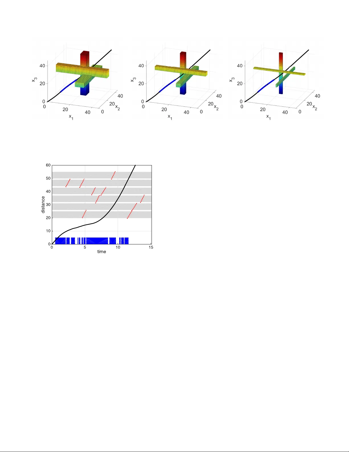
1 Safety V erificat ion and Control for Collision A v oidance a t Road Intersecti ons Heejin Ahn and Domitilla Del V ecchio Abstract —This paper presents the design of a supervisory algorithm that mo nitors safety at ro ad intersections and o v errides driver s with a safe input when necessary . The design of the supervisor consists of tw o parts: safety verification and contr ol design. Safety verification is the problem to determine if vehicles will be able to cr oss the intersection without colliding with curre nt driver s’ in puts. W e translate t his safety verification problem into a jobshop scheduling p roblem, which minimizes the maximum lateness and evaluates if the optimal cost is zero. Th e zero optimal cost corres ponds to the case in whi ch all vehicles can cross each conflict area without collisions. Computin g the optimal cost requires solving a Mixed Integer Nonli near Program ming (MINLP) problem due to the n onlinear second-order dynamics of the vehicles. W e theref ore estimate this optimal cost by formu- lating two related Mi xed In teger Linear Programm ing ( MILP) problems that assume simpler vehicle dynamics. W e prov e that these two MILP pr oblems yield lo wer and upper bounds of the optimal cost. W e also quantify the worst case approximation errors of these MILP problems. W e design the supervisor to ov erride the vehicles with a safe control i nput if the M ILP problem that computes the upper bou nd yields a positive optimal cost. W e theoretically demonstrate th at t he supervisor keeps the intersection sa fe and is non- blocking. Computer simulations further va lidate that the algorithms can run in rea l time f or problems of realistic size. Index T erms —safety verification; approximation; hybrid sys- tems; least r estrictiv e control; super visory contro l; collision a voidance; intersections; sch eduling; I . I N T RO D U C T I O N T HE first fatality cau sed b y a self-dr iving technolog y h as raised con cerns ab out the safety of auto nomo us vehicles [1]. As an appro ach to ensurin g safety particu larly at a r oad intersection, this pap er proposes the design of a safeguar d, called a sup ervisory algorith m or super visor . The superv isor monitors vehicles’ curr ent states and inputs through veh icle-to- vehicle and vehic le-to-infr astructure comm unications [2], an d determines if th eir in puts will cause collisions. If this is the case, the supervisor intervenes to prev ent collisions. Inform ally , we state safety verification a s a pr oblem tha t determines if the state trajec tory can be kept outside an unsafe set given an initial condition, where the un safe set is defined as the set o f states c orrespon ding to a collision configur ation. Reachability analysis has been used to solve this problem b y ca lculating the reachable r egion of a system to find a set of initial states that can be con trolled to av oid the unsafe set [ 3]–[5]. Ho wever , reachability an alysis of dyn amical This work was in part supported by NSF A ward #1239182. Heejin Ahn a nd Domitil la Del V ecchio are wi th the De partment of Me chani- cal Engineering, Massachusetts Institute of T echnology , 77 Massachusett s A v- enue, Cambridge, USA. Email: hja hn@mit.edu and ddv@mi t.edu Fig. 1. General inte rsectio n. The safety verificat ion problem in this scenario can be approximately solved within quantified bounds. This intersect ion is obtaine d from [15] to encompass 20 top crash locations in Massachusett s, USA. systems with la rge state spaces is u sually challengin g d ue to the co mplexity of co mputing rea chable sets. This motivates the development of se veral appr oximation appro aches. One approx imation appro ach is to consider a simpler dyn amical model to com pute reachable sets instead of using the origin al complex dynam ical model, as studied in [6]– [8]. Anoth er ap- proxim ation app roach is to appro ximate the orig inal r eachable set b y employing various geo metric rep resentations, which include poly hedra [9], ellipso ids [10], or p arallelotopes [11]. It has be en shown in [ 12] that mo noton icity of system dy namics, for which state trajector ies preserve a pa rtial or dering on states and in puts, makes the re achability analysis relatively simple. This is because f or such systems, the bou ndary of a reachable set can be c omputed by conside ring only m aximum and minimum states and inputs [ 13]. Indeed , an exact method for the reach ability analysis is presen ted in [14] for piecewise continuo us and monoto ne systems. Our app roach relies o n the m onoton icity of the system and on the a pprox imation of vehicle dynam ics. In this p aper, we consider complex intersection scenarios in which vehic les follow predefined paths as shown in Figure 1. T he long itudinal 2 dynamics of vehicles are piecewise continuou s and mo notone [14], which enables us to translate th e safety verification problem to a scheduling problem. Th is scheduling p roblem minimizes the max imum lateness and determine s if the optimal cost is zero . T he zero optim al co st implies that every job (vehicle) can be processed on each machine (conflict area) in time, and equ iv alently , vehicles can cross the inte rsection without collision . Howe ver , b ecause of the nonline ar seco nd- order dyn amics of vehicles, the scheduling prob lem is a Mixed Integer Nonlinear Pro grammin g (M INLP) pr oblem, which is computatio nally difficult to solve. W e th erefore estimate the op timal cost of the sch eduling prob lem by formu lating two Mixed In teger Linear Progr amming (MILP) pro blems that assume first-o rder d ynamics and no nlinear second-o rder dynamics o n a restricted inp ut set, respec ti vely . W e prove that th ese MIL P pro blems yield lower an d up per bo unds of the optimal cost. These lower and upper bou nd problem s are equiv alent to computing over- an d u nder-approx imation of th e reachable sets of the orig inal pro blem. Th ese appr oximation bound s are quantified in this paper . The scheduling p roblem has been emp loyed to solve the safety verificatio n prob lem for collision a voidance at an in ter- section [ 16]–[21]. In [1 6]–[20], the safety verification pr oblem is so lved exactly with an assumption th at the path s of vehicles intersect only at a single con flict point. Multiple conflict points are considered in [21] and the safety verification pr oblem is so lved exactly when vehicle dyn amics are r estricted to first-order linear dynam ics. By contrast, the main contribution of this paper is to solve the safety verification problem on multip le co nflict points fo r general lon gitudinal vehicle dynamics, which are nonlinear and second-o rder . A similar problem of robo ts f ollowing p redefined paths is consider ed in [22], [23], but their appro ach is not designed for safety verification and th us restricted to zer o initial speed with the double integrato r dynamics. Ou r schedu ling app roach can d eal with gener al vehicle d ynamics and verify safety at any given state. Recently , intersection man agement has been receiving con- siderable research attention. Mo st of the r ecent works co n- centrate on autonom ous intersection manag ement, wh ere a controller takes con trol o f vehic les at all times until they cr oss the intersection [24]–[30]. Our ap proach , instead, is to design a least restrictiv e sup ervisor in the sense th at it overrides drivers only when they cann ot avoid a collision. Collision avoidance for m ultiple vehicles has been an activ e area of research mostly in air traffic manag ement. V arious approx imation approac hes are employed to so lve collision av oid ance pr oblems, such as appr oximation of dy namics [31]– [36] or relaxation o f the original pr oblems [37], [38]. Th e controller s presented in these work s are no t least restrictive, as op posed to the con troller co nsidered in this pap er . While least restrictive con trollers are p resented in [ 3], [4], they ar e applicable o nly to a small num ber of vehicles due to the computatio nal complexity of safety verification. As a scalable approa ch with the number o f vehicles, dec entralized contr ol is also employed in [39]–[41]. However , d ecentralized con trol usually term inates with sub optimal solution s or deadlo ck. In this paper , we present the design of a centralized controller and 3 1 2 1 2 3 Fig. 2. An intersec tion is m odeled as a set of conflict areas near which two longitu dinal predefined paths intersec t. prove that it is non-b locking . W e validate thro ugh comp uter simulations that th is con troller can ru n in rea l time fo r realistic size scenarios such as that illustrated in Figu re 1. The rest of this p aper is organize d as follows. In Section II, we de fine an inter section mod el an d a veh icle dynam ic mo del. The saf ety verification problem is stated in Section III an d translated into a schedulin g pro blem in Sectio n IV. T o solve this pro blem, we form ulate th e lower an d upp er boun d pro b- lems an d q uantify the ir appr oximation bou nds in Section V. Based on the u pper bo und pro blem, a supe rvisory algorithm is in troduce d and proved to be n on-b locking in Sectio n VI. W e present simulation results in Section VII and conclu de the paper in Section VI II. I I . S Y S T E M D E FI N I T I O N A. Intersection Mod el At a road intersection , vehicles te nd to fo llow pred efined paths, which inter sect at sev eral c onflict poin ts. W e defin e an area aro und ea ch conflict po int accou nting fo r the len gth of vehicles and call it a conflict area. I n this p aper, we model an intersection as a collection of all conflict ar eas. For examp le, in Figure 2, the intersection is modeled as a set of conflict areas 1 -3. The main focus of this paper is to prevent co llisions among vehicles whose pa ths intersect at co nflict areas. T hus, we assume that the re is on ly one vehicle per lane an d neglect rear- end collision s. Th ese can be in cluded using a similar app roach as used in [17]. B. V ehicle Dyna mical Model W ith a vehicle state ( x j , ˙ x j ) where x j ∈ X j ⊆ R is the position o f vehicle j on its lon gitudinal path an d ˙ x j ∈ ˙ X j := [ ˙ x j,min , ˙ x j,max ] ⊂ R is the speed, th e longitudin al dynam ics of vehicle j ar e de scribed as fo llows: ¨ x j = f j ( x j , ˙ x j , u j ) . (1) The inp ut u j is th e throttle o r brake in put in the spac e U j := [ u j,min , u j,max ] ⊂ R . Let us conside r n vehicles app roachin g an in tersection. The whole system d ynamics can be o btained by com bining the individual dynamics (1) and written as follows: ¨ x = f ( x , ˙ x , u ) , (2) 3 where x = ( x 1 , . . . , x n ) ∈ X ⊆ R n and similarly , ˙ x ∈ ˙ X = [ ˙ x min , ˙ x max ] ⊂ R n , u ∈ U = [ u min , u max ] ⊂ R n . W e define an inp ut signal u j ( · ) : t ∈ R 7→ u j ( t ) ∈ U j in the input sign al space U j . Let x j ( t, u j ( · ) , x j (0) , ˙ x j (0)) denote th e position reach ed at time t starting fro m ( x j (0) , ˙ x j (0)) using an inpu t signal u j ( · ) ∈ U j . W e also use th e aggregate position x ( t, u ( · ) , x (0) , ˙ x (0)) with the aggregate inp ut signal u ( · ) ∈ U . Similarly , we use ˙ x ( t, u ( · ) , x (0) , ˙ x (0)) to den ote th e speed at time t ev o lving with u ( · ) . Regarding th ese, we make th e following assumption . Assumption 1 . F or all j ∈ { 1 , . . . , n } , the p osition x j ( t, u j ( · ) , x j (0) , ˙ x j (0)) depend s con tinuously on u j ( · ) ∈ U j , and the input signal space U j is p ath-con nected. W e say u j ( · ) ≤ u ′ j ( · ) ∈ U j if u j ( t ) ≤ u ′ j ( t ) ∈ U j for all t ≥ 0 . W e consider ˙ x j,min > 0 to exclude a trivial scenario in which vehicles come to a fu ll stop before an inter section and do not cross it. Most im portantly , we assum e that th e individual dy namics (1) are mono tone, th at is, they satisfy th e following prop erty . Assumption 2 . For all j ∈ { 1 , . . . , n } , if u j ( · ) ≤ u ′ j ( · ) , x j (0) ≤ x ′ j (0) , ˙ x j (0) ≤ ˙ x ′ j (0) , and t ≤ t ′ , x j ( t, u j ( · ) , x j (0) , ˙ x j (0)) ≤ x j ( t ′ , u ′ j ( · ) , x ′ j (0) , ˙ x ′ j (0)) for all t ≥ 0 . I I I . P RO B L E M S TA T E M E N T Let us consider n vehicles approach ing an in tersection th at is mod eled as a co llection of m co nflict areas. W e deno te the location of conflict area i on the long itudinal p ath o f vehicle j as an open interval ( α ij , β ij ) ⊂ R . W e say a collision oc curs at an intersection if two vehicles stay inside the sam e conflict area simu ltaneously . This configur ation is r eferred to as a bad set , which is denoted by B an d defined as fo llows: B := { x ∈ X : x j ∈ ( α ij , β ij ) a nd x j ′ ∈ ( α ij ′ , β ij ′ ) for some i ∈ { 1 , . . . , m } and j 6 = j ′ ∈ { 1 , . . . , n }} (3) The main intere st o f th is pape r is safety verification, th at is, verifying wheth er th e system can avoid entering the ba d set at all fu ture time. W e appro ach th is b y stating a math ematical problem , called the safety verification prob lem, as fo llows. Problem 1 ( safety verification) . Gi ven an initial cond ition ( x (0) , ˙ x (0)) , determ ine if th ere exists u ( · ) ∈ U such that x ( t, u ( · ) , x (0) , ˙ x (0)) / ∈ B f or all t ≥ 0 . T o a nswer th is problem , we need to ev aluate all p ossible input signals, wh ich are f unctions of time, until findin g o ne satisfying the conditio n. T o av oid this exha ustiv e and infinite set of computa tions, we translate this prob lem to a schedu ling problem , which is to find feasible sched ules, n on-negative r eal number s, fo r vehicles to cross the conflict ar eas. The ratio nale behind this translation is that real numbers are computationally less comp licated to m anipulate than fun ctions. While this scheduling pr oblem is still no t easy to solve, we can provid e its appr oximate solution s efficiently . 1,1 2,2 3,3 3,1 1,2 2,3 (a) 2,2 3,1 1,2 2,3 (b) Fig. 3. (a) All operations of the scenario in Figure 2. (b) Operatio ns when β 11 ≤ x 1 (0) < β 31 , x 2 (0) < β 22 , and β 33 ≤ x 3 (0) < β 23 . See Example 1 for m ore details. I V . S C H E D U L I N G : E Q U I V A L E N T P RO B L E M T O P RO B L E M 1 In th is sectio n, we formu late a scheduling pr oblem and present the theorem stating that this p roblem is equiv alent to the safe ty verification p roblem (Pro blem 1). A schedulin g problem can b e describ ed by a graph rep re- sentation [42]. For a no de, let ( i, j ) be an oper ation of vehicle j processing on co nflict area i . Th e collection of all o perations is d enoted by ¯ N . ¯ N := { ( i, j ) ∈ { 1 , . . . , m } × { 1 , . . . , n } : conflict area i is on the rou te of vehicle j } . W e also d efine a set N ⊆ ¯ N that contains op erations to be processed g iv en an initial p osition x (0) . N := { ( i, j ) ∈ ¯ N : x j (0) < β ij } . Recall that ( α ij , β ij ) ⊂ R denotes the location of conflict area i on the lo ngitudin al path of vehicle j . No tice that N is the set of all the oper ations o f interest giv en x (0) because β ij ≤ x j (0) indicates that vehicle j has exited c onflict area i . A first operatio n set F ⊆ N and a last o peration set L ⊆ N are d efined as follows: F := { ( i, j ) ∈ N : ( i, j ) is the first operation o f vehicle j } , L := { ( i, j ) ∈ N : ( i, j ) is the last operation of vehicle j } . Now , let us define arcs in the graph . W e d efine sets o f conjunc ti ve a rcs C and disjunctive ar cs D , which connect two operation s in N as f ollows: C := { ( i, j ) → ( i ′ , j ) : vehicle j crosses conflict area i and then conflict area i ′ for some i, j, j ′ } , D := { ( i, j ) ↔ ( i, j ′ ) : vehicles j an d j ′ share the sam e conflict area i for some i, j, j ′ } . That is, an elemen t in C represen ts th e sequence of operatio ns on the path of a vehicle, an d an elemen t in D rep resents the undeterm ined sequence of op erations o n the same conflict area. Example 1. In the scenario in Fig ure 2, sup pose β 11 ≤ x 1 (0) < β 31 , x 2 (0) < β 22 , and β 33 ≤ x 3 (0) < β 23 . The operation s are illu strated in Figure 3, where the operatio n sets ¯ N an d N b ecome as f ollows: ¯ N = { (1 , 1 ) , (3 , 1) , (2 , 2) , (1 , 2) , (3 , 3 ) , (2 , 3) } , N = { (3 , 1 ) , (2 , 2) , (1 , 2) , (2 , 3) } . 4 Here, the first and last operation sets are F = { (3 , 1) , (2 , 2) , (2 , 3 ) } , L = { (3 , 1) , (1 , 2) , (2 , 3 ) } . The sets of conjunc ti ve and disjunctiv e arcs are C = { (2 , 2 ) → (1 , 2 ) } and D = { (2 , 2 ) ↔ (2 , 3 ) } . W e now intro duce sche duling parameter s, release times, deadlines, and pr ocess times, to f ormulate a jobsho p schedul- ing problem [42]. Giv en an initial con dition ( x j (0) , ˙ x j (0)) , let T ij be the time that vehicle j will enter conflict area i , th at is, x j ( T ij , u j ( · ) , x j (0) , ˙ x j (0)) = α ij for some u j ( · ) ∈ U j . Let T b e the set of T ij for all ( i, j ) ∈ N . A job shop scheduling problem is to find this set, c alled a sched ule, such that vehicles never m eet inside a conflict area. Giv en T , the release time R ij ( T ) is the soonest time at which vehicle j can en ter conflict ar ea i un der the constrain t that it enters the previous co nflict area i ′ at T i ′ j . Th e dead line D ij ( T ) is the latest such time. The pro cess time P ij ( T ) is the min imum time th at vehicle j takes to exit conflict are a i und er the con straint th at it en ters the same conflict area at time T ij and the next co nflict ar ea i ′′ at time T i ′′ j . W e omit the argumen t T if it is clear f rom co ntext. Formally , the release time and deadline are de fined as follows. Gi ven an in itial cond ition ( x (0) , ˙ x (0)) and T , for all ( i, j ) ∈ N \ F , there is a preceding op eration ( i ′ , j ) such that ( i ′ , j ) → ( i, j ) ∈ C . R ij ( T ) := min u j ( · ) ∈U j { t : x j ( t, u j ( · ) , x j (0) , ˙ x j (0)) = α ij with constrain t x j ( T i ′ j , u j ( · ) , x j (0) , ˙ x j (0)) = α i ′ j } , D ij ( T ) := max u j ( · ) ∈U j { t : x j ( t, u j ( · ) , x j (0) , ˙ x j (0)) = α ij with constrain t x j ( T i ′ j , u j ( · ) , x j (0) , ˙ x j (0)) = α i ′ j } . (4) If the co nstraint is n ot satisfied, set R ij = ∞ and D ij = − ∞ . For all ( i, j ) ∈ F , such a preced ing operatio n ( i ′ , j ) d oes no t exists. If x j (0) < α ij , R ij := min u j ( · ) ∈U j { t : x j ( t, u j ( · ) , x j (0) , ˙ x j (0)) = α ij } , D ij := max u j ( · ) ∈U j { t : x j ( t, u j ( · ) , x j (0) , ˙ x j (0)) = α ij } . (5) If α ij ≤ x j (0) , set R ij = D ij = 0 . Notice that f or ( i, j ) ∈ F , the release time and dead line are indep endent of T . The process time is d efined as f ollows. Gi ven an initial condition ( x (0) , ˙ x (0)) and T , for all ( i, j ) ∈ N \ L , there is a succeeding o peration ( i ′′ , j ) such that ( i, j ) → ( i ′′ , j ) ∈ C . If x j (0) < α ij , P ij ( T ) := min u j ( · ) ∈U j { t : x j ( t, u j ( · ) , x j (0) , ˙ x j (0)) = β ij with constrain ts x j ( T ij , u j ( · ) , x j (0) , ˙ x j (0)) = α ij and x j ( T i ′′ j , u j ( · ) , x j (0) , ˙ x j (0)) = α i ′′ j } . (6) Set P ij ( T ) := min u j ( · ) ∈U j { t : x j ( t, u j ( · ) , x j (0) , ˙ x j (0)) = β ij with con straint x j ( T i ′′ j , u j ( · ) , x j (0) , ˙ x j (0)) = α i ′′ j } if α ij ≤ x j (0) < β ij . For all ( i, j ) ∈ L , such a succeed ing operation ( i ′′ , j ) does not exist. If x j (0) < α ij , P ij ( T ) := min u j ( · ) ∈U j { t : x j ( t, u j ( · ) , x j (0) , ˙ x j (0)) = β ij with constrain t x j ( T ij , u j ( · ) , x j (0) , ˙ x j (0)) = α ij } . (7) If α ij ≤ x j (0) < β ij , set P ij := min u j ( · ) ∈U j { t : x j ( t, u j ( · ) , x j (0) , ˙ x j (0)) = β ij } . If β ij ≤ x j (0) , operation ( i, j ) is not of in terest since vehicle j h as already crossed conflict area i . If the constra ints are no t satisfied, set P ij = ∞ . Using the definition s above, a jobshop scheduling prob lem is f ormulated as follows. Problem 2 (jobsho p scheduling pr oblem) . Given an initial condition ( x (0) , ˙ x (0)) , d etermine if s ∗ = 0 : s ∗ := minimize T , k max ( i,j ) ∈N ( T ij − D ij ( T ) , 0) subject to for all ( i, j ) ∈ N , R ij ( T ) ≤ T ij , (P2.1) for all ( i, j ) ↔ ( i, j ′ ) ∈ D ,      P ij ( T ) ≤ T ij ′ + M (1 − k ij j ′ ) , P ij ′ ( T ) ≤ T ij + M (1 − k ij ′ j ) , k ij j ′ + k ij ′ j = 1 . (P2.2) where T = { T ij : ( i, j ) ∈ N } , k = { k ij j ′ ∈ { 0 , 1 } : for all ( i, j ) ↔ ( i, j ′ ) ∈ D } , and M > 0 is a large numb er . In th e sched uling literature, max( T ij − D ij ( T ) , 0) is called the m aximum laten ess. This cost indicates the existence of a schedule that vio lates the d eadline, and thus its minimization is o ne of the most studied schedu ling pro blems [42]. If s ∗ = 0 , we ha ve T ij that satisfies T ij ≤ D ij ( T ) for all ( i, j ) ∈ N . The fact that T ij is bound ed by R ij ( T ) and D ij ( T ) encodes the bounds of the inp ut. Constraint (P2.2) says that for two vehicles j a nd j ′ that share the same co nflict area i , either vehicle j ′ enters it after vehicle j exits (when k ij j ′ = 1 ) or the other way ar ound ( when k ij ′ j = 1 ). By this co nstraint, each conflict area is exclusiv ely used by on e vehicle at a time. Thus, the existence of such T and k that yield s ∗ = 0 is equivalent to the existence of u ( · ) ∈ U to avoid the bad set. This is th e essence o f the pr oof of the following theorem. Theorem 1 ( [21]) . Pr oblem 1 is eq uivalent to Pr oblem 2. In [21], Problem 2 was in troduced as a feasibility pro blem and the above theorem was pr oved. Theorem 1 implies th e following: g iv en an initial conditio n ( x (0) , ˙ x (0)) , s ∗ = 0 = ⇒ a safe in put signal exists to av oid B , s ∗ > 0 = ⇒ no safe in put signal exists to avoid B . That is, s ∗ is the indicator of the vehicles’ safety . While this theor em hold s fo r g eneral d ynamics (1), Prob- lem 2 can be difficult to solve dep ending on which vehicle dy - namics are considered . In [21], vehicle dynamics are a ssumed to b e first-o rder and lin ear in wh ich case Prob lem 2 be comes a Mixed In teger Linear Pr ogramm ing (MI LP) prob lem, which can be easily solved by a co mmercially av ailab le solver , such as CPLEX [4 3]. In this paper, due to the n onlinear and higher order vehicle dynam ics, the constraints are nonline ar in T ij and therefo re, Prob lem 2 is a Mixed Integer Non- Linear Program ming (MI NLP) problem, wh ich is notoriou s for its com putational intractab ility . T o approx imately solve 5 Problem 2, we f ormulate two M ILP prob lems th at yield lower and upper bo unds o f s ∗ , respectiv ely . The M ILP problem that computes the lower boun d is a ref ormulation of the MILP problem given in [21], and the MIL P problem tha t comp utes the u pper boun d is based o n n onlinear second-o rder d ynamics with a limited input space. V . A P P RO X I M AT E S O L U T I O N S T O P RO B L E M 2 In this sectio n, we p rovide two M ILP pro blems that yield lower and upper bounds o f the o ptimal co st o f Problem 2. Using th ese bo unds, we can qu antify the appro ximation error between the appr oximate solution and th e exact solution to Problem 2 . A. Lower b ound pr oble m Let us conside r first-ord er vehicle dynam ics, that is, ˙ χ = v , where χ ∈ X is the vector r epresenting the position of vehicles on their lon gitudinal paths, and v is the in put. Th e input v lies in the space ˙ X = [ ˙ x min , ˙ x max ] with ˙ x min > 0 . W e also define an inp ut signal v j ( · ) : R + → ˙ X j in th e spac e V j for vehicle j . W e define r elease times an d d eadlines fo r th e lower boun d problem . Process times are con sidered as d ecision variables. Definition 1. Given an initial con dition ( x (0) , ˙ x (0)) and χ (0) = x (0) , re lease times r ij and deadlines d ij are defined as follows. For all ( i, j ) ∈ F , if x j (0) < α ij , r ij := min u j ( · ) ∈U j { t : x j ( t, u j ( · ) , x j (0) , ˙ x j (0)) = α ij } , d ij := max u j ( · ) ∈U j { t : x j ( t, u j ( · ) , x j (0) , ˙ x j (0)) = α ij } . If α ij ≤ x j (0) , then r ij = d ij = 0 . For ( i , j ) ∈ N \ F , the re exists a preceding operation ( i ′ , j ) such that ( i ′ , j ) → ( i, j ) ∈ C . Given p i ′ j ≥ 0 such that χ j ( p i ′ j , v j ( · ) , χ j (0)) = β i ′ j for som e v j ( · ) ∈ V j , r ij := p i ′ j + α ij − β i ′ j ˙ x j,max , d ij := p i ′ j + α ij − β i ′ j ˙ x j,min . (8) Notice that for the first operation s, ( i, j ) ∈ F , release times and de adlines con sider gen eral dy namics (1) and thus r ij = R ij and d ij = D ij by (5). This is a d ifferent defin ition from that in [2 1] and resu lts in a tig hter con straint than r ij = ( α ij − χ j (0)) / ˙ x j,max and d ij = ( α ij − χ j (0)) / ˙ x j,min . Using Definition 1, the lower bound proble m is formu lated as a d ecision problem in whic h the maximu m lateness is minimized. Problem 3 (lower bo und prob lem) . Giv en an in itial c ondition ( x (0) , ˙ x (0)) , determ ine if s ∗ L = 0 : s ∗ L := m inimize t , p , k max ( i,j ) ∈N ( t ij − d ij , 0) subject to for all ( i, j ) ∈ N , r ij ≤ t ij , (P3.1) for all ( i, j ) ∈ N , β ij − α ij ˙ x j,max ≤ p ij − t ij ≤ β ij − α ij ˙ x j,min , (P3.2) for all ( i, j ) ↔ ( i, j ′ ) ∈ D ,      p ij ≤ t ij ′ + M (1 − k ij j ′ ) , p ij ′ ≤ t ij + M (1 − k ij ′ j ) , k ij j ′ + k ij ′ j = 1 . (P3.3) where t = { t ij : ( i, j ) ∈ N } , p = { p ij : ( i, j ) ∈ N } , k := { k ij j ′ ∈ { 0 , 1 } : for all ( i, j ) ↔ ( i, j ′ ) ∈ D } and M is a large numb er in R + . From (8), we know th at the objec ti ve function and con- straint (P3.1) are linear with the decision variables. Thu s, this pr oblem is a M ixed Integer Linear Pr ogramm ing (MILP) problem . Theorem 2. s ∗ L ≤ s ∗ Pr oof: Suppose Problem 2 find s T ∗ and k ∗ with the correspo nding cost s ∗ , wheth er or not s ∗ = 0 . W e will show that ˜ t = T ∗ and ˜ k = k ∗ become a feasible solution for Problem 3 with som e ˜ p . Giv en T ∗ , we have P ij ( T ∗ ) for all ( i, j ) ∈ N . Consider ˜ p ij = P ij ( T ∗ ) . From (6) and (7), P ij ( T ∗ ) − T ∗ ij = ˜ p ij − ˜ t ij is th e time to reach β ij from α ij and thus satisfies (P3.2). Constraint (P3.3) is the s ame as constraint (P2.2) in Problem 2 . W e will show that r ij ≤ R ij ( T ∗ ) and D ij ( T ∗ ) ≤ d ij . As mentioned e arlier , for ( i, j ) ∈ F , r ij = R ij and d ij = D ij . For ( i , j ) ∈ N \ F , we h av e a p receding operatio n ( i ′ , j ) such that ( i ′ , j ) → ( i, j ) ∈ C . By (4), R ij is eq ual to T ∗ i ′ j plus the m inimum time to r each α ij from α i ′ j . Con sidering th is definition wi th (6), R ij is again eq ual t o P i ′ j plus the minimum time to reach α ij from β i ′ j , thereby R ij ≥ P i ′ j + ( α ij − β i ′ j ) / ˙ x j,max . Also, sinc e P i ′ j = ˜ p i ′ j , we have P i ′ j + ( α ij − β i ′ j ) / ˙ x j,max = r ij . Thus r ij ≤ R ij . Similarly , D ij ≤ d ij . By these inequ alities, R ij ≤ T ∗ ij implies r ij ≤ T ∗ ij = ˜ t ij , which is co nstraint (P3.1). Therefo re, ˜ t , ˜ p , and ˜ k is a feasible solution of Pro blem 3. Since D ij ≤ d ij , s ∗ L ≤ max( ˜ t ij − d ij , 0) ≤ max( T ∗ ij − D ij , 0) = s ∗ . B. Upper b ound pr ob lem In this section, we relax Proble m 2 to a MILP pro blem by considerin g gener al dynam ics (1) on a restricted inpu t space. This p roblem is to find a set of times a t which vehicles en ter their first confl ict ar ea , assuming that to reach th e following conflict areas all vehicles app ly m aximum in put. Th e ra tionale here is tha t once a vehicle enter s an intersection, the dri ver tries to exit as soon as p ossible. W e define α j,min to d enote the first con flict area as fo llows: α j,min := min ( i,j ) ∈ ¯ N α ij . Recall that ¯ N is a set of all operation s ind epende nt o f an initial condition . 6 (a) x j (0) < α j,min = α i ′ j (b) α i ′ j ≤ x j (0) < β i ′ j Fig. 4. Illustration of Definitions 2 and 3. Suppose ( i ′ , j ) ∈ F and ( i ′ , j ) → ( i, j ) ∈ C . W e can compute ¯ P i ′ j , ¯ T ij , ¯ P ij by considering the maximum input inside the intersect ion. In the uppe r bou nd pro blem, th e time to reach the first conflict area is a decision variable, as opp osed to Problem s 2 and 3 who se decision variables are the e ntering tim es f or all conflict areas. This decision variable, called a sched ule, is denoted by T F = { T F ij : f or all ( i, j ) ∈ F } and defined as x j ( T F ij , u j ( · ) , x j (0) , ˙ x j (0)) = α ij for some u j ( · ) ∈ U j if x j (0) < α ij and otherwise T F ij = 0 . The r elease times and dead lines are defined only fo r the first operation as follows. Definition 2. Given a n initial con dition ( x (0) , ˙ x (0)) , release times ¯ R = { ¯ R ij : fo r a ll ( i, j ) ∈ F } and deadlin es ¯ D = { ¯ D ij : fo r all ( i, j ) ∈ F } a re d efined as follows. For all ( i, j ) ∈ F , if x j (0) < α j,min , ¯ R ij := min u j ( · ) ∈U j { t : x j ( t, u j ( · ) , x j (0) , ˙ x j (0)) = α j,min } , ¯ D ij := max u j ( · ) ∈U j { t : x j ( t, u j ( · ) , x j (0) , ˙ x j (0)) = α j,min } . (9) If α j,min ≤ x j (0) < α ij , ¯ R ij := min u j ( · ) ∈U j { t : x j ( t, u j ( · ) , x j (0) , ˙ x j (0)) = α ij } , ¯ D ij = ¯ R ij . (10) If α ij ≤ x j (0) , set ¯ R ij = ¯ D ij = 0 . Notice that ¯ R ij = R ij and ¯ D ij = D ij if x j (0) < α j,min , and ¯ D ij = ¯ R ij = R ij if x j (0) ≥ α j,min . Th e release time ¯ R ij and the dead line ¯ D ij depend on ly on an in itial con dition ( x j (0) , ˙ x j (0)) , not on the decision variable T F ij . Giv en a sch edule T F , we define ¯ T = { ¯ T ij : fo r all ( i , j ) ∈ N } and ¯ P = { ¯ P ij : fo r all ( i, j ) ∈ N } as illustrated in Figure 4. Suppose vehicle j ha s the first operation ( i ′ , j ) . When vehicle j is outside the intersectio n ( x j (0) < α j,min ) , ¯ T ij and ¯ P ij represent th e min imum times at which vehicle j can en ter an d exit co nflict are a i , respectively , no matter wha t speed it ha s at T F i ′ j . When vehicle j is inside the intersection ( α j,min ≤ x j (0)) , ¯ T ij and ¯ P ij are the m inimum times at which it enter s and exits c onflict a rea i , r espectively . The se are f ormally defined as follows. Definition 3. Given an initial condition ( x (0) , ˙ x (0)) and a schedule T F , we defin e ¯ T = { ¯ T ij : for all ( i, j ) ∈ N } and ¯ P = { ¯ P ij : fo r all ( i, j ) ∈ N } a s f ollows. If x j (0) < α j,min , for ( i, j ) ∈ F , ¯ T ij = T F ij , (11) ¯ P ij = T F ij + min u j ( · ) ∈U j { t : x j ( t, u j ( · ) , α ij , ˙ x j,min ) = β ij } , and for ( i, j ) ∈ N \ F , there exists the first operation ( i ′ , j ) such that ( i ′ , j ) ∈ F an d α i ′ j = α j,min . ¯ T ij = T F i ′ j + min u j ( · ) ∈U j { t : x j ( t, u j ( · ) , α j,min , ˙ x j,max ) = α ij } , ¯ P ij = T F i ′ j + min u j ( · ) ∈U j { t : x j ( t, u j ( · ) , α j,min , ˙ x j,min ) = β ij } . (12) If α j,min ≤ x j (0) , for ( i, j ) ∈ F , ¯ T ij = T F ij , ¯ P ij = T F ij − ¯ R ij + min u j ( · ) ∈U j { t : x j ( t, u j ( · ) , x j (0) , ˙ x j (0)) = β ij } . (13) and for ( i, j ) ∈ N \ F , there exists the first operation ( i ′ , j ) such that ( i ′ , j ) ∈ F . ¯ T ij = T F i ′ j − ¯ R i ′ j + min u j ( · ) ∈U j { t : x j ( t, u j ( · ) , x j (0) , ˙ x j (0)) = α ij } , ¯ P ij = T F i ′ j − ¯ R i ′ j + min u j ( · ) ∈U j { t : x j ( t, u j ( · ) , x j (0) , ˙ x j (0)) = β ij } . (14) In (13) an d (14), we have ¯ R ij = ¯ D ij by (10) a nd thus f or ( i ′ , j ) ∈ F , T F i ′ j − ¯ R i ′ j = 0 if T F i ′ j ∈ [ ¯ R i ′ j , ¯ D i ′ j ] . Using these definition s, we formulate the upper boun d problem . Problem 4 ( upper bound prob lem) . Giv en an in itial c ondition ( x (0) , ˙ x (0)) , determ ine if s ∗ U = 0 : s ∗ U := m inimize T F , k max ( i,j ) ∈F ( T F ij − ¯ D ij , 0) subject to for all ( i, j ) ∈ F , ¯ R ij ≤ T F ij , (P4.1) for all ( i, j ) ↔ ( i, j ′ ) ∈ D ,      ¯ P ij ≤ ¯ T ij ′ + M (1 − k ij j ′ ) , ¯ P ij ′ ≤ ¯ T ij + M (1 − k ij ′ j ) , k ij j ′ + k ij ′ j = 1 . (P4.2) where T F = { T F ij : for all ( i, j ) ∈ F } , k = { k ij j ′ ∈ { 0 , 1 } : for all ( i, j ) ↔ ( i, j ′ ) ∈ D } , and M is a la rge num ber in R + . The con straints in the p roblem are written in linear form s with the decision variable T F as noticed in (1 1)-(14). Thus, the p roblem is a MILP prob lem. W e will show that s ∗ U in Problem 4 can b e co nsidered as an upper bound o f s ∗ in Pro blem 2 in the sense that s ∗ ≤ M s ∗ U for a large n umber M > 0 . This ine quality is not trivial if s ∗ U = 0 . In th e following thereom, there fore, we will show that s ∗ U = 0 implies s ∗ = 0 fo r any initial con dition ( x (0) , ˙ x (0)) . Theorem 3. s ∗ U = 0 ⇒ s ∗ = 0 . 7 Pr oof: Sup pose Pr oblem 4 finds an optimal solution T F ∗ = { T F ∗ ij : ( i, j ) ∈ F } and k ∗ = { k ∗ ij j ′ : ( i, j ) ↔ ( i, j ′ ) ∈ D } that yields s ∗ U = 0 . W e define ˜ T an d ˜ P as follows. For ( i, j ) ∈ F , if x j (0) < α ij , ˜ T ij = T F ∗ ij , ˜ P ij = T F ∗ ij + min u j ( · ) ∈U j { t : x j ( t, u j ( · ) , α ij , ˙ x 0 j ) = β ij } , (15) where ˙ x 0 j = ˙ x j ( T F ∗ ij , u j ( · ) , x j (0) , ˙ x j (0)) with α ij = x j ( T F ∗ ij , u j ( · ) , x j (0) , ˙ x j (0)) . If x j (0) ≥ α ij , let ˜ T ij = T F ∗ ij = 0 and ˜ P ij = min { t : x j ( t, u j ( · ) , x j (0) , ˙ x j (0)) = β ij } . For ( i , j ) ∈ N \ F , there exists the first o peration ( i ′ , j ) ∈ F , and ˜ T ij = T F ∗ i ′ j + min u j ( · ) ∈U j { t : x j ( t, u j ( · ) , α i ′ j , ˙ x 0 j ) = α ij } , ˜ P ij = T F ∗ i ′ j + min u j ( · ) ∈U j { t : x j ( t, u j ( · ) , α i ′ j , ˙ x 0 j ) = β ij } , (16) where ˙ x 0 j = ˙ x j ( T F ∗ i ′ j , u j ( · ) , x j (0) , ˙ x j (0)) with α i ′ j = x j ( T F ∗ i ′ j , u j ( · ) , x j (0) , ˙ x j (0)) . Notice that ˜ P ij is P ij ( ˜ T ) by (6) and (7). W e will show that ˜ T an d ˜ k = k ∗ is a feasible solution to Prob lem 2. First, we will show th at ˜ T satisfies constraint (P2.1) in Problem 2. For all ( i, j ) ∈ F , ¯ R ij = R ij and ¯ D ij ≤ D ij . Since T F ∗ ij satisfies constraint (P4.1), we have R ij ≤ ˜ T ij . For ( i, j ) ∈ N \ F , we d efine ˜ T ij as th e min imum time to reach conflict area i , thereb y ˜ T ij = R ij ( ˜ T ) by ( 4). Th is establishes that R ij ≤ ˜ T ij for all ( i, j ) ∈ N . For constraint (P2.2) in Problem 2, let us focu s on (15), (16), and Definition 3 giv en T F ∗ . If x j (0) < α j,min , we have ¯ T ij ≤ ˜ T ij and ˜ P ij ≤ ¯ P ij because ¯ T ij and ¯ P ij are comp uted with the m aximum and m inimum speed, respectively . If x j (0) ≥ α j,min , for ( i ′ , j ) ∈ F we h av e T F ∗ i ′ j = ¯ R i ′ j since s ∗ U = 0 and ¯ R i ′ j = ¯ D i ′ j . Th is imp lies that ¯ T ij = ˜ T ij and ¯ P ij = ˜ T ij . Thus, constraint (P4.2) beco mes ˜ P ij ≤ ¯ P ij ≤ ¯ T ij ′ + M (1 − k ∗ ij j ′ ) ≤ ˜ T ij ′ + M (1 − k ∗ ij j ′ ) , ˜ P ij ′ ≤ ¯ P ij ′ ≤ ¯ T ij + M (1 − k ∗ ij ′ j ) ≤ ˜ T ij + M (1 − k ∗ ij ′ j ) . That is, ˜ T and ˜ k = k ∗ satisfy constrain t ( P2.2) in Problem 2. Now we have a feasible solution ˜ T an d ˜ k . For ( i, j ) ∈ N \ F , we have ˜ T ij = R ij ≤ D ij , and thus, max ( i,j ) ∈N \F ( ˜ T ij − D ij , 0) = 0 . For ( i, j ) ∈ F , we hav e ¯ D ij ≤ D ij and the following inequa lities comp lete the pro of. s ∗ ≤ max ( i,j ) ∈N ( ˜ T ij − D ij , 0) = max ( i,j ) ∈F ( ˜ T ij − D ij , 0) ≤ ma x ( i,j ) ∈F ( ˜ T ij − ¯ D ij , 0) = s ∗ U . Therefo re, if s ∗ U = 0 , we h ave s ∗ = 0 . By Theore ms 2 and 3, we have s ∗ L > 0 ⇒ s ∗ > 0 and s ∗ U = 0 ⇒ s ∗ = 0 . That is, fro m Proble ms 3 an d 4 , wh ich can be solved with a commercia l solver such as CPLEX, we can find th e solution for Problem 2 as shown in T able I. Howe ver, when s ∗ L = 0 and s ∗ U > 0 , repre sented b y Case II in the table, s ∗ is not ex- actly determ ined. In this case, we will provide approx imation bound s. T ABLE I S U M M A RY O F T H E O R E M S 2 A N D 3 s ∗ L s ∗ U s ∗ Case I · 0 0 Case II 0 + ? Case III + · + C. Ap pr oxima tion bo unds W e exactly solve Prob lem 2 in cases I and III as noted in T ab le I, but h av e to approximate the solution in case II . In this section, we will focu s o n the latter case when s ∗ L = 0 and s ∗ U > 0 and qu antify th e ap proxim ation bounds. Notice that s ∗ L > 0 and s ∗ U = 0 can not occur . W e will prove the f ollowing statemen t: if s ∗ L = 0 and s ∗ U > 0 , an inp ut exists that makes the system av o id a shrun k bad set but not an inflated bad set . These bad sets a re defined indepen dent of time and thus we con sider N = ¯ N . A shrunk conflict ar ea and an in flated co nflict area are defined in the fo llowing definitions. See Figure 5. Definition 4 . A shru nk conflict area ( ˆ α ij , ˆ β ij ) for all ( i, j ) ∈ N is defined as fo llows. For all ( i, j ) ∈ F , ˆ α ij = α ij , ˆ β ij = min u j ( · ) ∈U j x j  β ij − α ij ˙ x j,max , u j ( · ) , α ij , ˙ x j,min  . (17) For all ( i, j ) ∈ N \ F , th ere exists the first operation ( i ′ , j ) for i 6 = i ′ such that ( i ′ , j ) ∈ F . ˆ α ij = max u j ( · ) ∈U j x j  α ij − α i ′ j ˙ x j,min , u j ( · ) , α i ′ j , ˙ x j,max  , ˆ β ij = min u j ( · ) ∈U j x j  β ij − α i ′ j ˙ x j,max , u j ( · ) , α i ′ j , ˙ x j,min  . (18) If ˆ α ij ≥ ˆ β ij , set ( ˆ α ij , ˆ β ij ) a s an empty set. Definition 5. An inflated conflict area ( ˇ α ij , ˇ β ij ) fo r all ( i, j ) ∈ N is defined as fo llows. For all ( i, j ) ∈ F , ˇ α ij = α ij , ˇ β ij = max u j ( · ) ∈U j x j ( t ∗ , u j ( · ) , α ij , ˙ x j,max ) , (19) where t ∗ = min u j ( · ) ∈U j { t : x j ( t, u j ( · ) , α ij , ˙ x j,min ) = β ij } and α ij = α j,min . For all ( i, j ) ∈ N \ F , ˇ α ij = min u j ( · ) ∈U j x j ( t ∗∗ , u j ( · ) , α j,min , ˙ x j,min ) , ˇ β ij = max u j ( · ) ∈U j x j ( t ∗∗∗ , u j ( · ) , α j,min , ˙ x j,max ) , (20) where t ∗∗ = min u j ∈U j { t : x j ( t, u j ( · ) , α j,min , ˙ x j,max ) = α ij } and t ∗∗∗ = min u j ∈U j { t : x j ( t, u j ( · ) , α j,min , ˙ x j,min ) = β ij } . Notice th at t ∗ , t ∗∗ , and t ∗∗∗ are th e same as the add ed times in (1 1) and (12). A shrunk b ad set ˆ B an d an inflated bad set ˇ B ar e defined as follows: ˆ B := { x ∈ X : f or some ( i, j ) ↔ ( i , j ′ ) ∈ D x j ∈ ( ˆ α ij , ˆ β ij ) and x j ′ ∈ ( ˆ α ij ′ , ˆ β ij ′ ) } . (21) 8 (a) (b) t * (c) t ** t *** (d) Fig. 5. Shrunk and Inflated conflict areas for ( i ′ , j ) ∈ F and ( i ′ , j ) → ( i, j ) ∈ C . Figures (a)-(d) illustrate (17)-(20), respecti vely . By definition, ( ˆ α i ′ j , ˆ β i ′ j ) ⊆ ( α i ′ j , β i ′ j ) ⊆ ( ˇ α i ′ j , ˇ β i ′ j ) and ( ˆ α ij , ˆ β ij ) ⊆ ( α ij , β ij ) ⊆ ( ˇ α ij , ˇ β ij ) . ˇ B := { x ∈ X : for some ( i, j ) ↔ ( i , j ′ ) ∈ D x j ∈ ( ˇ α ij , ˇ β ij ) and x j ′ ∈ ( ˇ α ij ′ , ˇ β ij ′ ) } . (22) It can be checked that ˆ B ⊆ B ⊆ ˇ B by showing that ( ˆ α ij , ˆ β ij ) ⊆ ( α ij , β ij ) ⊆ ( ˇ α ij , ˇ β ij ) f or all ( i, j ) ∈ N . In th e fo llowing theore ms, we prove th at the shrunk and inflated b ad sets can r epresent the approxim ation erro rs of the solutions of Pro blems 3 a nd 4, respectively . More precisely , we prove th at 1) if the solution of Problem 3 is yes , that is, s ∗ L = 0 , then there exists an inpu t that makes the sy stem avoid the shr unk b ad set, and 2) if the solu tion of Prob lem 4 is no , that is, s ∗ U > 0 , then th ere is no inpu t that m akes the system av oid the inflated b ad set. Theorem 4. Given a n initial condition ( x (0) , ˙ x (0)) , if s L ∗ = 0 , then there exists an in put signal u ( · ) ∈ U suc h that x ( t, u ( · ) , x (0) , ˙ x (0)) / ∈ ˆ B for all t ≥ 0 . Pr oof: If s ∗ L = 0 , ther e exists an optimal solutio n t ∗ , p ∗ and k ∗ that satisfies t ∗ ij ≤ d ij for all ( i, j ) ∈ N a nd constraints (P3.1)-(P3.3) in Prob lem 3. For ( i , j ) ∈ F , r ij ≤ t ∗ ij ≤ d ij implies that th ere exists u ∗ j ( · ) : [0 , t ∗ ij ) → U j such that x j ( t ∗ ij , u ∗ j ( · ) , x j (0) , ˙ x j (0)) = α ij = ˆ α ij (23) since the flow o f x j is a continu ous f unction of u ∗ j ( · ) and the input space is path conn ected by Assum ption 1. Le t ˙ x j ( t ∗ ij ) denote ˙ x j ( t ∗ ij , u ∗ j ( · ) , x j (0) , ˙ x j (0)) . Constraint ( P3.2), ( β ij − α ij ) / ˙ x j,max ≤ p ∗ ij − t ∗ ij ≤ ( β ij − α ij ) / ˙ x j,min , implies that for any in put u ∗ j ( · ) : [ t ∗ ij , p ∗ ij ) → U j , x j ( p ∗ ij − t ∗ ij , u ∗ j ( · ) , α ij , ˙ x j ( t ∗ ij )) ≥ ˆ β ij , (24) because ˆ β ij defined in (17) is th e min imum distance fr om α ij trav eled for time ( β ij − α ij ) / ˙ x j,max . For ( i , j ) ∈ N \ F , there exists the first o peration ( i ′ , j ) ∈ F . By th e d efinition of r ij and d ij in (8), we have t ∗ i ′ j + α ij − α i ′ j ˙ x j,max ≤ r ij ≤ t ∗ ij ≤ d ij ≤ t ∗ i ′ j + α ij − α i ′ j ˙ x j,min . Since ˆ α ij is th e max imum d istance from α i ′ j trav eled for time ( α ij − α i ′ j ) / ˙ x j,min , for any input u ∗ j ( · ) : [ t ∗ i ′ j , t ∗ ij ) → U j , x j ( t ∗ ij − t ∗ i ′ j , u ∗ j ( · ) , α i ′ j , ˙ x j ( t ∗ i ′ j )) ≤ ˆ α ij . (25) Similarly for any inpu t u ∗ j ( · ) : [ t ∗ i ′ j , p ∗ ij ) → U j , x j ( p ∗ ij − t ∗ i ′ j , u ∗ j ( · ) , α i ′ j , ˙ x j ( t ∗ i ′ j )) ≥ ˆ β ij . (26) Thus, ther e exists an inp ut u ∗ j ( · ) ∈ U j that satisfies ( 23)-(26). Now we will show that x ( t, u ∗ ( · ) , x (0) , ˙ x (0)) / ∈ ˆ B f or all t ≥ 0 . By (P3.3), we ha ve for ( i, j ) ↔ ( i, j ′ ) ∈ D either p ∗ ij ≤ t ∗ ij ′ or p ∗ ij ′ ≤ t ∗ ij . W ith out loss of generality , we consider p ∗ ij ≤ t ∗ ij ′ . Then, at time t ∗ ij ′ , vehicle j ′ has n ot y et entered shrunk conflict are a i as shown in (23) an d (25). At the sam e time, vehicle j has already exited the shr unk conflict area as shown in ( 24) and (2 6). Thus, two vehicles n ev er meet inside the same shrunk co nflict area, a nd thu s the system avoids th e shrunk bad set with the input signal u ∗ ( · ) . Theorem 5. Given a n initial cond ition ( x (0) , ˙ x (0)) , if s ∗ U > 0 , then fo r all in put signal u ( · ) ∈ U , x ( t, u ( · ) , x (0) , ˙ x (0)) ∈ ˇ B for some t ≥ 0 . Pr oof: W e prove the contra-po sition: if there exists an input sign al u ∗ ( · ) ∈ U such tha t x ( t, u ∗ ( · ) , x (0) , ˙ x (0)) / ∈ ˇ B for all t ≥ 0 , then s ∗ U = 0 . For all ( i, j ) ∈ N , let us d efine T ∗ ij := { t : x j ( t, u ∗ j ( · ) , x j (0) , ˙ x j (0)) = ˇ α ij } , if x j (0) < ˇ α ij . Otherwise, set T ∗ ij = 0 . Also, if x j (0) < ˇ β ij , P ∗ ij := { t : x j ( t, u ∗ j ( · ) , x j (0) , ˙ x j (0)) = ˇ β ij } . Otherwise, set P ∗ ij = 0 . Since x ( t, u ∗ ( · ) , x (0) , ˙ x (0)) / ∈ ˇ B for all t ≥ 0 , we have for all ( i, j ) ↔ ( i, j ′ ) ∈ D , ( T ∗ ij , P ∗ ij ) ∩ ( T ∗ ij ′ , P ∗ ij ′ ) = ∅ , (27) which indicates that each inflated co nflict area is occupied by only o ne vehicle at a time . Let u s define a sched ule ˜ T F = { ˜ T F ij : for all ( i, j ) ∈ F } as follows: if x j (0) < α j,min , ˜ T F ij := { t : x j ( t, u ∗ j ( · ) , x j (0) , ˙ x j (0)) = α j,min } . If α j,min ≤ x j (0) , set ˜ T F ij = ¯ R ij . By Definition 2, ˜ T F ij ∈ [ ¯ R ij , ¯ D ij ] . Th us, ˜ T F satisfies con straint (P4.1) and ˜ T F ij − ¯ D ij ≤ 0 f or all ( i, j ) ∈ F . If ˜ T F satisfies constraint (P4.2), ˜ T F is a feasible solutio n to Problem 4 with a corresp onding binary variable ˜ k = { ˜ k ij j ′ : fo r all ( i, j ) ↔ ( i, j ′ ) ∈ D } and thus s ∗ U = 0 . 9 Giv en ˜ T F , ¯ T = { ¯ T ij : for all ( i, j ) ∈ N } and ¯ P = { ¯ P ij : for all ( i, j ) ∈ N } ar e defined accordin g to Definition 3. First, consider x j (0) < α j,min . For ( i, j ) ∈ F , we have by (11), ¯ T ij = ˜ T F ij and ¯ P ij = ˜ T F ij + t ∗ where t ∗ is intro duced in ( 19). Since ˇ α ij ≤ α j,min by defin ition, T ∗ ij ≤ ¯ T ij . Also, since ˇ β ij represents the maxim um distance from α j,min that vehicle j can travel during t ∗ , traveling from α j,min to ˇ β ij takes no less time than t ∗ . Thu s, ¯ P ij ≤ P ∗ ij . For ( i, j ) ∈ N \ F , there exists ( i ′ , j ) ∈ F . By (12), ¯ T ij = ˜ T F i ′ j + t ∗∗ and ¯ P ij = ˜ T F i ′ j + t ∗∗∗ , where t ∗∗ and t ∗∗∗ are in troduce d in (2 0). Since ˇ α ij and ˇ β ij are the minimu m an d max imum distance trav eled fr om α j,min for time t ∗∗ and t ∗∗∗ , re spectiv ely , we have T ∗ ij ≤ ¯ T ij and ¯ P ij ≤ P ∗ ij . Next, consider α j,min ≤ x j (0) . In this case, ¯ R ij = ¯ D ij for all vehicle j ’ s oper ations b y (10) and thus for ( i ′ , j ) ∈ F , we have ˜ T F i ′ j = ¯ R i ′ j . By (13), ¯ T i ′ j = ˜ T F i ′ j and ¯ P i ′ j is th e minimum time to r each β ij since ˜ T F i ′ j − ¯ R i ′ j = 0 . T he fact that ˇ α ij ≤ α ij and β ij ≤ ˇ β ij implies T ∗ ij ≤ ¯ T ij and ¯ P ij ≤ P ∗ ij , respectively . For ( i, j ) ∈ N \ F , ¯ T ij and ¯ P ij are the min imum time to rea ch α ij and β ij , respectively , starting from x j (0) . Since ¯ T ij ≥ ( α ij − x j (0)) / ˙ x j,max and ˇ α ij is the m inimum distance traveled in ( α ij − x j (0)) / ˙ x j,max , T ∗ ij ≤ ¯ T ij . Also, β ij ≤ ˇ β ij implies ¯ P ij ≤ P ∗ ij . Therefo re, ( ¯ T ij , ¯ P ij ) ⊆ ( T ∗ ij , P ∗ ij ) for all ( i, j ) ∈ N . By (27), we d erive ( ¯ T ij , ¯ P ij ) ∩ ( ¯ T ij ′ , ¯ P ij ′ ) = ∅ for all ( i, j ) ↔ ( i, j ′ ) ∈ D . T his is equiv alent to con straint ( P4.2), and thus there exists ˜ k ij j ′ and ˜ k ij ′ j satisfying the constraint. Therefo re, ˜ T F and ˜ k is a feasible solution with s ∗ U = 0 . By Theor em 4, if Problem 3 r eturns yes , there is an input to m ake the system av oid the shrunk b ad set. Otherwise, n o input exists to m ake the system av oid th e ba d set. Similarly for Proble m 4, if it return s yes , there is an input to make the system a void the bad set. O therwise, n o in put exists to av oid the inflated bad set by Theorem 5. Thu s, the shrunk an d inflated bad sets represent the over-approximation and un der- approx imation of the r eachable set f rom an initial con dition ( x (0) , ˙ x (0)) , respectively . D. Oth er upper bou nd solutions In Section V -B, we formulate a n MILP problem that yields an upp er bo und by consider ing th e m aximum inpu t in side an intersection. Different M ILP formulatio ns are po ssible, for example, by considering th e minimum input inside an i ntersec- tion. T o obtain a tighter upp er b ound, various com binations o f the maxim um and m inimum inputs can b e considered inside an inter section with a binary variable associated with each combinatio n. At the expense of com putational com plexity , this approa ch is less conservati ve since more ch oices o f inputs are allowed. V I . C O N T RO L D E S I G N Based on the r esults of Section V, we c an design a sup ervi- sor th at is activ ated when a f uture co llision is detected inside the inflated conflict areas. Let A P P RO X V E R I FI C AT I O N ( x (0) , ˙ x (0)) be an algo rithm solving Problem 4 giv en an initial cond ition ( x (0) , ˙ x (0)) . Let A P P RO X V E R I FI C A T I O N retur n ( s ∗ U , T F ∗ ) where T F ∗ is th e optimal solution. The super visory alg orithm run s in discrete time with a time step τ . At time k τ , it r eceiv es the m easurements of the state ( x ( k τ ) , ˙ x ( k τ )) and the desired inpu t u k d ∈ U , which is a vector of inpu ts that the dr iv ers are app lying at the time . Th ese measuremen ts are u sed to predict the desired state at the next time step, which is deno ted by ( x k d , ˙ x k d ) . W e solve Problem 4 to see if th e desired state has a safe input signal within the approx imation bound . If A P P ROX V E R I FI C AT I O N ( x k d , ˙ x k d ) retur ns T F ∗ that makes s ∗ U = 0 , we can find a safe inpu t signal by defining an input generato r function σ : X × ˙ X × R n → U as follows: σ ( x k d , ˙ x k d , T F ∗ ) ∈ { u ( · ) ∈ U : f or all ( i, j ) ∈ F , x j ( T F ∗ ij , u j ( · ) , x k j,d , ˙ x k j,d ) = α ij and u j ( t ) = u j,max ∀ t ≥ T F ∗ ij } , where x k j,d and ˙ x k j,d denote the j -th en tries of x k d and ˙ x k d , respectively . The sup ervisor stores this safe input restricted to time (0 , τ ) for a possible use at the next time step . Since ther e is an in put signal that m akes the system av o id en tering the b ad set f rom ( x k d , ˙ x k d ) , the superv isor allows the desired in put. If A P P RO X V E R I FI C A T I O N ( x k d , ˙ x k d ) retur ns s ∗ U > 0 , the supervisor overrides the drivers with the safe inp ut stored at the previous step. Th is safe inpu t is used to p redict the safe state, denoted by ( x k saf e , ˙ x k saf e ) , and this safe state is used to generate a safe in put fo r the next time step. W e will p rove in the next theorem that A P P RO X V E R I FI C A T I O N ( x k saf e , ˙ x k saf e ) always return s s ∗ U = 0 an d thus a safe input signal is defined. This superv isor is provided in Algorithm 1. An input signal with superscr ipt k , such a s u k ( · ) , den otes an input fun ction from [0 , τ ) to U . W e defin e the desired inpu t signal as u k d ( · ) : t 7→ u k d giv en u k d ∈ U . Also, an inp ut sign al with su perscript k , ∞ indicates that the dom ain of the in put signal is [0 , ∞ ) . Algorithm 1 Sup ervisory control algorithm at t = k τ 1: procedure S U P E RV I S O R ( x ( k τ ) , ˙ x ( k τ ) , u k d ) 2: x k d ← x ( τ , u k d ( · ) , x ( kτ ) , ˙ x ( k τ )) 3: ˙ x k d ← ˙ x ( τ , u k d ( · ) , x ( kτ ) , ˙ x ( k τ )) 4: ( s ∗ U , T F ∗ 1 ) = A P P R OX V E R I FI C AT I O N ( x k d , ˙ x k d ) 5: if s ∗ U = 0 then 6: u k +1 , ∞ saf e ( · ) ← σ ( x k d , ˙ x k d , T F ∗ 1 ) 7: u k +1 saf e ( · ) ← u k +1 , ∞ saf e ( t ) f or t ∈ [0 , τ ) 8: return u k d ( · ) 9: else 10: x k saf e ← x ( τ , u k saf e ( · ) , x ( kτ ) , ˙ x ( k τ )) 11: ˙ x k saf e ← ˙ x ( τ , u k saf e ( · ) , x ( kτ ) , ˙ x ( k τ )) 12: ( · , T F ∗ 2 ) = A P P R OX V E R I FI C AT I O N ( x k saf e , ˙ x k saf e ) 13: u k +1 , ∞ saf e ( · ) ← σ ( x k saf e , ˙ x k saf e , T F ∗ 2 ) 14: u k +1 saf e ( · ) ← u k +1 , ∞ saf e ( t ) f or t ∈ [0 , τ ) 15: return u k saf e ( · ) By Th eorem 5, s ∗ U > 0 ind icates that no inp ut signal exists to avoid the inflated bad set, that is, there may exist an input to avoid the b ad set. Thu s, we say this sup ervisor overrides vehicles when a futu re collision is detected within the ap prox imation boun d. 10 Theorem 6. Algorithm 1 is non-blocking, tha t is, if S U P E RV I S O R ( x (0) , ˙ x (0) , u 0 d ) 6 = ∅ , then for any u k d ∈ U , S U P E RV I S O R ( x ( k τ ) , ˙ x ( k τ ) , u k d ) 6 = ∅ . Pr oof: W e pr ove this by induction o n k . For the base case, assume S U P E RV I S O R ( x (0) , ˙ x (0) , u 0 d ) 6 = ∅ an d u 1 , ∞ saf e ( · ) is well-defined, tha t is, u 1 , ∞ saf e ( · ) ∈ U . Suppose at time ( k − 1) τ , S U P E RV I S O R ( x (( k − 1) τ ) , ˙ x (( k − 1) τ ) , u k − 1 d ) is non- empty an d u k, ∞ saf e is well- defined. At time k τ , fo r any u k d ∈ U , S U P E RV I S O R ( x ( k τ ) , ˙ x ( k τ ) , u k d ) is n ot empty since it r eturns either u k d ( · ) : t 7→ u k d or u k saf e ( · ) : t 7→ u k, ∞ saf e ( t ) . W e need to show that u k +1 , ∞ saf e ( · ) is well-defined in lines 6 or 13. In lin e 6, since T F ∗ 1 = { T F ∗ ij, 1 : ( i, j ) ∈ F } yields s ∗ U = 0 , we hav e ¯ R ij ≤ T F ∗ ij, 1 ≤ ¯ D ij for all ( i, j ) ∈ F an d thu s there exists u j ( · ) ∈ U j that satisfies x j ( T F ∗ ij, 1 , u j ( · ) , x k j,d , ˙ x k j,d ) = α ij . Th us, σ ( x k d , ˙ x k d , T F ∗ 1 ) is well-define d. In line 13, we will sh ow th at T F ∗ 2 satisfies s ∗ U = 0 and th us a safe inp ut signal is well- defined. W e h av e th at ( x ( k τ ) , ˙ x ( k τ )) is either ( x k − 1 d , ˙ x k − 1 d ) or ( x k − 1 saf e , ˙ x k − 1 saf e ) de- pending o n th e ou tput of the superviso r at th e p revious time step. Thus, at time ( k − 1 ) τ , A P P ROX V E R I FI C A - T I O N ( x ( k τ ) , ˙ x ( k τ )) yielde d s ∗ U = 0 with an optim al solution T F ,k − 1 = { T F ,k − 1 ij : ( i, j ) ∈ F } . L et ¯ R k − 1 ij , ¯ D k − 1 ij , ¯ T k − 1 ij , and ¯ P k − 1 ij be th e parameter s used in the problem . Now , co n- sider A P P RO X V E R I FI C AT I O N ( x k saf e , ˙ x k saf e ) with p arameters ¯ R k ij , ¯ D k ij , ¯ T k ij , a nd ¯ P k ij . If we define ˜ T F ij = T F ,k − 1 ij − τ fo r all ( i, j ) ∈ F , we have ˜ T F ij ∈ [ ¯ R k ij , ¯ D k ij ] since T F ,k − 1 ij ∈ [ ¯ R k − 1 ij , ¯ D k − 1 ij ] an d u k saf e ( · ) is in U . Also, since ( ¯ T k ij , ¯ P k ij ) ⊆ ( ¯ T k − 1 ij , ¯ P k − 1 ij ) − τ and ( ¯ T k − 1 ij , ¯ P k − 1 ij ) ∩ ( ¯ T k − 1 ij ′ , ¯ P k − 1 ij ′ ) = ∅ for all ( i, j ) ↔ ( i, j ′ ) ∈ D , we have ( ¯ T k ij , ¯ P k ij ) ∩ ( ¯ T k ij ′ , ¯ P k ij ′ ) = ∅ . Therefo re, ˜ T F = { ˜ T F ij : fo r all ( i, j ) ∈ F } is a feasible solu- tion that yields s ∗ U = 0 , an d th us th ere exists the optimal solu- tion T F ∗ 2 satisfying s ∗ U = 0 . T herefor e, σ ( x saf e , ˙ x saf e , T F ∗ 2 ) is we ll-defined. V I I . S I M U L AT I O N R E S U LT S W e implemented Algo rithm 1 on the cases illustra ted in Figures 1 an d 2 to validate its co llision av oidance p erform ance and its non-b locking pr operty . W e imp lemented th e algorithm on MA TLAB and perform ed simulations on a persona l com- puter consisting of an Intel Core i7 processor at 3.10 GHz and 8 GB RAM. In the simu lations, we consider the vehicle dyn amics with a quadr atic drag term [44] as follows: for all j ∈ { 1 , . . . , n } ¨ x j = au j + b ˙ x 2 j . Also, the fo llowing param eters are used: τ = 0 . 1 , a = 1 , b = 0 . 0 05 . For all j ∈ { 1 , . . . , n } , u j,max = 2 , u j,min = − 2 , α j,min = 20 . For all ( i, j ) ∈ N , β ij − α ij = 5 and for all ( i, j ) → ( i ′ , j ) ∈ C , α i ′ j − α ij = 6 . Let us co nsider the scenar io illustrated in Figure 2 with the following initial condition and parameter s: x (0) = (0 , 0 , 0) , ˙ x (0) = (10 , 8 , 8 ) , an d ˙ x j,min = 8 , ˙ x j,max = 1 0 for all j ∈ { 1 . . . , n } . W ith out imp lementing the super visor (Algorithm 1), we let the vehicles travel with the desired inp ut u k d = ( − 2 , − 2 , 2) for all k and plot the optimal v alues of Fig. 6. Simulati on results without the supervisor (Algorithm 1) for the scenari o in Figure 2. Cases I, II, and III denote the same cases in T able I. Problems 3 and 4. These are shown in Figure 6. As p roved in Theor ems 2 and 3, s ∗ U = 0 imp lies s ∗ L = 0 . Th e trajectory of the system with impleme nting the sup ervisor is shown in Figure 7(a)-(c). The trajectory (b lack lin e) is contro lled b y th e supervisor wh en s ∗ U > 0 (th e line is thicker in blue ) so that it av o ids the b ad set (solid in (b )). Notice that the trajectory penetrates the inflated bad set (solid in (a)) but n ot th e shru nk bad set (solid in (c)) as proved in Th eorems 4 and 5. Now , let us consider the scenario illu strated in Figu re 1 with th e following in itial condition an d p arameters: x (0) = (0 , − 2 , 5 , − 5 , 0 , 5 , 0 , 1 , 5 , 4 , 0 , − 2 , 5 , 5 , 0 , 5 , − 2 , 0 , − 2 , 0) and for all j ∈ { 1 , . . . , n } , ˙ x j (0) = 5 , ˙ x j,min = 1 , ˙ x j,max = 10 . W ith th e d esired input u k d = u max for all k , th e resu lt is shown in Fig ure 8. The trajecto ry of vehicle 1 (black line) a nd the trajectories of oth er vehicles that share th e same co nflict area (red d otted lines) never stay inside the conflict area simultaneo usly . This implies that the sup ervisor overrides vehicles when necessary (when blue b oxes ap pear) to make them cross the intersection without collisions. Because unnecessary to prove o ptimality , solving feasibility pro blems requires less computation al effort th an solving optimization problem s [4 3]. That is, solvin g the following proble m takes less comp utation time th an solving Problem 4: given an initial condition , determine if there exists a feasible solution ( T F , k ) that satisfies (P4.1), ( P4.2), and T F ij ≤ ¯ D ij for all ( i, j ) ∈ F . Notice th at th is pro blem is equiv alen t to Problem 4. Based on the solution of this feasibility p roblem , Algorith m 1 takes no mor e than 0. 05 s p er iteration, e ven in this realistic size scenario in volving 20 vehicles, 48 conflict areas, and 120 oper- ations on a represen tativ e g eometry of danger ous intersections. Giv en tha t the a llocated time step for in telligent transporta tion systems is 0 .1 s [ 2], this alg orithm can b e implemen ted in real time. V I I I . C O N C L U S I O N S In this pap er , we pre sented the d esign of a sup ervisory algo- rithm that d etermines th e existence of a future collision amo ng vehicles at an in tersection (safety verification) an d overrides the d rivers with a safe inp ut if a f uture collision is dete cted 11 (a) Inflated bad set ˇ B (b) Bad set B (c) Shrunk bad set ˆ B Fig. 7. Simulation results w ith the supervisor for the scenario in Figure 2. The black line represents the system trajectory and is the same on each figure. The line turns to blue when the supervisor intervene s to pre vent a predicted collision . The solid in each fi gure is (a) the inflated bad set, (b) the bad set, and (c) the shrunk bad set. The supervisor manages the system to avoid entering the bad set. Fig. 8. Traje ctory of vehicle 1 in the scenario of Figure 1 crossing six conflict areas. The blue boxes represe nt the times at which the supervi sor overri des the vehicle s. The red dotted line s are the trajector ies of the other vehicle s that share the same confli ct area. This graph sho ws that each confli ct area is used by only one vehi cle at a time. (contro l design ). W e translated the safety verification pr oblem into a schedu ling problem by explo iting mon otonicity o f the system. This sche duling problem minimize s the maximum lateness and determines if the optimal cost is zero where the zero op timal co st corr esponds to the case in which all vehicles can cro ss th e intersection witho ut collisions. Because of th e nonlinear second -order dyn amics o f vehicle s, the sched uling problem is a Mixed I nteger No nlinear Pr ogramm ing (MI NLP) problem , which is co mputation ally d ifficult to solve. W e thus approx imately solved this scheduling prob lem b y solving two Mixed In teger Linear Program ming (MILP) pr oblems that yield lower and upper boun ds of the optimal cost of the scheduling p roblem. W e qu antified th e appr oximation erro r between the exact and ap proxim ate solutions to th e schedulin g problem . W e p resented th e design of the supervisor based on the MI LP prob lem th at com putes th e up per boun d a nd proved that it is non -blockin g. Computer simulatio ns validated that the superv isor can be implemen ted in real time a pplications. While we assum ed in this paper that there is only one vehicle per lane, our appro ach can be easily modified to deal with the case in which multiple vehicles a re p resent o n eac h lane. One possible m odification can be solvin g the scheduling problem only for the first vehicles on lanes while letting the following vehicles m aintain a safe d istance from their f ront vehicles. I nstead of this naive app roach, we are currently in ves- tigating a less conser vati ve appr oach. Also, Problem 4 can be extended to include th e p resence of uncertain ty sources, such as measuremen t n oises, proc ess errors, and not commu nicating vehicles, as don e in our previous works [18 ], [19] for the single conflict a rea intersection model. Also, in future work, the assumption that the routes of vehicles are known in advance will be r elaxed. R E F E R E N C E S [1] E. Acker man, “Fata l T esla self-dri ving car crash reminds us that robots aren’t perfect, ” Jul. 2016. [Online]. A v ailab le: http:/ /spectru m.ieee.org /cars- that- think/transportation/self- driving/fatal- tesla- autopilot- c r a s h - r e m i n d s - u s - t h a t - r o b o t s - a r e n t - p e r f e c t [2] U.S. Department of Transporta tion, “ITS Strategic research plan 2015- 2019, ” http://www .its.dot.go v/strat egicplan.pdf , 2014. [3] C. T omlin, G. J. Pappas, and S. Sastry , “Conflict resolution for air traf fic management : a study in multiage nt hybrid systems, ” IEEE T ransactio ns on Automatic Contr ol , vol. 43, no. 4, pp. 509–521, Apr . 1998. [4] C. T omlin, J. L ygeros, and S. Sastry , “ A game theoretic approach to control ler design for hybrid systems, ” Pr oceedi ngs of the IEEE , vo l. 88, no. 7, pp. 949–970, J ul. 2000. [5] J. L ygeros, C. T omlin, and S. Sastry , “Cont rollers for reachabil ity specifica tions for hybrid systems, ” Automati ca , vol. 35, no. 3, pp. 349– 370, Mar . 1999. [6] T . A. Henzi nger , P .-H. Ho, and H. W ong-T oi, “ Algorithmic analysis of nonline ar hybrid s ystems, ” IEEE Tr ansactions on Automati c Contr ol , vol. 43, no. 4, pp. 540–554, Apr . 1998. [7] R. Alur , T . Dang, and F . Iv ani, “Predicate abstract ion for reachabilit y analysi s of hybrid systems, ” ACM Tr ansactions on Embedded Computi ng Systems , vol. 5, no. 1, pp. 152–199, Feb . 2006. [8] A. Girard, A. A. Julius, and G. J. Pappas, “ Approximate simulation relati ons for hybrid s ystems, ” Discrete Event Dynamic Systems , vol. 18, no. 2, pp. 163–179, Oct. 2007. [9] E. Asarin, O. Bournez , T . Dang, and O. Male r , “ Approximate reachabil- ity anal ysis of piece wise-linea r dynamical systems, ” in Hybrid Syste ms: Computati on and Contr ol . Springer , Mar . 2000, no. 1790, pp. 20–31. [10] P . Gagarinov and A. A. Kur zhanskiy , “Ellipsoida l T oolbox, ” 2014. [On- line]. A vaila ble: http://systema nalysisdpt - c mc- ms u.github .io/ellipsoids/ [11] T . Dreossi, T . D ang, and C. Piazz a, “Paralle lotope bundle s for poly- nomial reachabi lity , ” in P r oc. 19th International Confer ence on Hybrid Systems: Computation and Contr ol (HSCC) . A CM, 2016, pp. 297–306. 12 [12] T . Moor and J. Raisch, “ Abstracti on based supervisory controller synthe- sis for hi gh order monoton e continuous systems, ” in Model ling , A nalysis, and Design of Hybrid Systems . Springer , 2002, no. 279, pp. 247–265. [13] D . Del V ecchio, M. Malisof f, and R. V erma, “ A separation principle for a class of hybrid automata on a partial order , ” in Pr oc. American Contr ol Confer ence (ACC) , 2009, pp. 3638–3643. [14] M. R. Hafner and D. Del V ec chio, “Computat ional tools for the safety control of a class of piece wise continu ous systems with imperfec t infor - mation on a partial order , ” SIAM Jou rnal on Contr ol and Optimization , vol. 49, pp. 2463–2493, 2011. [15] Massachusetts Department of Transportat ion, “2012 T op Crash Location s Report, ” 2014. [Online]. A va ilabl e: https:/ /www .massdot.state.ma.us/Portal s/8/docs/traf fic/CrashData/12T opCrashLocationsRpt.pdf [16] A . Colombo and D. Del V ecchi o, “Effic ient algorithms for collisi on av oidanc e at intersec tions, ” in Pr oc. 15th internation al confer ence on Hybrid Systems: Computation and Contr ol (HSCC) . A CM, 2012, pp. 145–154. [17] ——, “Least restricti ve supervisors for intersecti on collision avoi dance: A schedul ing approach, ” IEE E T ra nsactions on Au tomatic Contr ol , 2014. [18] L . Bruni, A. Colombo, and D. Del V ecchi o, “Rob ust multi-age nt colli sion avo idance through schedul ing, ” in P r oc. IEEE Confer ence on Decision and Contr ol (CDC) , Dec. 2013, pp. 3944–3950. [19] H . Ahn, A. Colombo, and D. Del V ec chio, “Supervisory control for in- tersect ion collisi on av oidance in the presence of uncontrolled vehicl es, ” in Proc . American Contr ol Confere nce (ACC ) , Jun. 2014, pp. 867–873. [20] H . Ahn, A. Rizzi, A. Colombo, and D. Del V ecc hio, “Experimental test - ing of a semi-auton omous multi-v ehicl e collisi on avo idance algorithm at an intersecti on testbed, ” in Pr oc. IEEE/RSJ Internat ional Confere nce on Intellige nt Robots and Systems (IR OS) , Sep. 2015, pp. 4834–4839. [21] H . Ahn and D. Del V ecchi o, “Semi-aut onomous intersection colli sion av oidanc e through job-shop scheduling, ” in Pro c. 19th International Confer ence on Hybrid Systems: Computation and Contr ol (HSCC) . A CM, A pr . 2016, pp. 185–194. [22] J . Peng and S. Akella, “Coordinatin g Multiple Double Integrat or Robots on a Roadmap: Con vex ity and Global Optimality , ” in Proc. IEE E Internati onal Confe re nce on Robotic s and Automation (ICRA) , Apr . 2005, pp. 2751–2758. [23] ——, “Coordinati ng multipl e robots with kinodynamic constraints along specified path s, ” The Interna tional Jo urnal of Robotic s Researc h , vol. 24, no. 4, pp. 295–310, Apr . 2005. [24] K .-D. Kim and P . Kumar , “ An MPC-based approach to prov able system- wide safety and liv eness of auton omous ground traf fi c, ” IEEE T ransac- tions on Aut omatic Contr ol , vol. 59, no. 12, pp. 3341–3356, Dec. 2014. [25] M. Kamal, J. Imura, T . Hayakaw a, A. Ohata, and K. Aihara, “ A V ehic le- Intersec tion Coordina tion Scheme for Smooth Flo ws of Traf fic W ithout Using Traf fic L ights, ” IEEE T ransactions on Intell ige nt T ransportat ion Systems , 2014. [26] F . Z hu and S. V . Ukkusuri, “ A linear programming formulation for autonomous intersection control within a dynamic traf fic assignment and connect ed vehic le en vironment, ” T ransport ation Researc h P art C: Emergi ng T echnol ogie s , vol . 55, pp. 363–378, Jun. 2015. [27] N . Murgo vski, G. R. de Campos, and J . Sj ¨ oberg , “Con ve x modeling of conflict resolu tion at traf fic intersecti ons, ” in Pr oc. IEEE Confer ence on Decision and Contr ol (CDC) , Dec. 2015, pp. 4708–4713. [28] L . Chen and C. Englund, “Cooperati ve intersectio n management : A sur- ve y , ” IEEE T ransact ions on Intelli gent T ransportatio n Systems , vol. 17, no. 2, pp. 570–586, F eb 2016. [29] R. T achet, P . Santi, S. Sobole vsky , L . I. Reye s-Castro, E. Frazzoli, D. Helbing , and C. Ratti, “Re visiting street intersecti ons using slot-based systems, ” P LoS ONE , vol. 11, no. 3, p. e0149607, Mar . 2016. [30] F . Altch´ e, X . Qian, and A. de La Fortel le, “T ime-opti mal coordination of mobile robots along specifie d paths, ” 2016. [Online]. A v ailable: http:/ /arxi v . org/a bs/1603.04610 [31] A . Richards, T . Schouwenaa rs, J. P . How , and E. Feron, “Spacecra ft Tra jector y Planning with A voidance Constraint s Using Mixed -Inte ger Linear Programming, ” Journal of Guidance , Contr ol, and Dynamics , vol. 25, no. 4, pp. 755–764, 2002. [32] L . Pallotti no, E. Feron, and A. Bicchi , “Conflict resolut ion problems for air traffic management systems solved with mixed inte ger program- ming, ” IEE E T ransact ions on Intellig ent T ransportatio n Systems , vol . 3, no. 1, pp. 3–11, Mar . 2002. [33] A . E. V ela, S. Solak, J. P . B. Cla rke, W . E. Singhose, E. R. Barnes, and E. L. Johnson, “Near real-time fuel-opti mal en route conflict resolution, ” IEEE T ransactions on Intellige nt T ransportat ion Syste ms , v ol. 11, no. 4, pp. 826–837, Dec. 2010. [34] A . Alonso-A yuso, L. Escudero, and F . Martn-Campo, “Collisio n A void- ance in Air Traf fic Management: A Mixed-Int eger Linear Optimization Approach, ” IEEE T ransactions on Intellig ent T ransportat ion Systems , vol. 12, no. 1, pp. 47–57, Mar . 2011. [35] A . Alonso-A yuso, L. F . Escudero, and F . J. Martn-Ca mpo, “On modeling the air traffic control coordinatio n in the coll ision a void ance problem by mixed integer linear optimiz ation, ” Annals of Operations Resear ch , vol. 222, no. 1, pp. 89–105, Mar . 2013. [36] J . Om er , “ A space-discre tized mixed-i nteg er linea r model for air -conflict resoluti on w ith speed and hea ding maneuvers, ” Compute rs & Operatio ns Resear ch , vol. 58, pp. 75–86, Jun. 2015. [37] M. Soler , M. Kamgarpour , J . Lloret, and J. L ygeros, “ A hybrid optimal control approa ch to fuel-ef ficient aircraft conflict av oidance , ” IEEE T ransaction s on Intellig ent Tr ansportation Systems , vol. 17, no. 7, pp. 1826–1838, Jul. 2016. [38] W . Chen, J. Chen, Z. Shao, and L. T . Bie gler , “Three-dimensi onal aircra ft conflict resoluti on based on smoothing methods, ” Journal of Guidance , Contr ol, and Dynamics , vol. 39, no. 7, pp. 1481–1490, 2016. [39] L . Pall ottino, V . Scordio, A. Bicchi , and E. Frazzoli, “Decentra lize d Cooperat i ve Policy for Conflict Resolut ion in Multi vehi cle Systems, ” IEEE T ransac tions on Robotics , vol . 23, no. 6, pp. 1170–1183, Dec. 2007. [40] T . Ke viczky , F . Borrelli, K. Fregene, D. G odbole, and G. J. Balas, “Decen traliz ed receding horizon control and coor dinati on of auton omous vehi cle formations, ” IEEE T ransactions on Contr ol Syst ems T echno logy , vol. 16, no. 1, pp. 19–33, 2008. [41] W . Zhang, M. Kamgarpou r , D. Sun, and C. J. T omlin, “ A hierarchic al flight plannin g frame work for air traffic manageme nt, ” Pr oceedi ngs of the IEEE , vol. 100, no. 1, pp. 179–194, Jan. 2012. [42] M. Pinedo, Schedu ling , 4th ed. Springer , 2012. [43] IBM Corporation, “CPLEX User’ s Manual , ” 2015. [Online]. A v ailab le: http:/ /www .ibm.com/support/kno wledgecenter/SSSA5P 12.6.3/ilog.odms.studi o.help/pd f / u s r c p l e x . p d f [44] M. Hafner , D. Cunning ham, L. Caminit i, and D. Del V ecchio, “Cooper- ati ve colli sion av oidance at intersections: algorit hms and experi ments, ” IEEE T ransactions on Intellige nt T ransportation Systems , vol. 14, no. 3, pp. 1162–1175, 2013.