Bayesian Learning-Based Adaptive Control for Safety Critical Systems

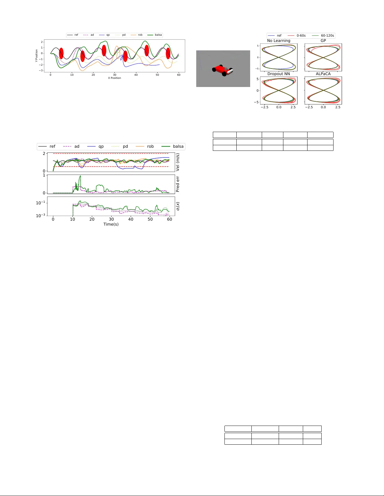
Bayesian Learning-Based Adaptiv e Control f or Safety Critical Systems David D. Fan 1 , 3 , Jennifer Nguyen 2 , Rohan Thakker 3 , Nikhilesh Alatur 3 , Ali-akbar Agha-mohammadi 3 , and Ev angelos A. Theodorou 1 Abstract — Deep learning has enjoyed much recent success, and applying state-of-the-art model learning methods to con- trols is an exciting prospect. However , there is a strong reluctance to use these methods on safety-critical systems, which hav e constraints on safety , stability , and r eal-time performance. W e propose a framework which satisfies these constraints while allowing the use of deep neural networks for learning model uncertainties. Central to our method is the use of Bayesian model lear ning, which pro vides an avenue f or maintaining ap- propriate degrees of caution in the face of the unknown. In the proposed approach, we develop an adaptive control framework leveraging the theory of stochastic CLFs (Control L yapunov Functions) and stochastic CBFs (Control Barrier Functions) along with tractable Bayesian model learning via Gaussian Processes or Bayesian neural networks. Under reasonable assumptions, we guarantee stability and safety while adapting to unknown dynamics with probability 1. W e demonstrate this architecture for high-speed terrestrial mobility targeting potential applications in safety-critical high-speed Mars rover missions. Index T erms — Robust/Adaptive Control of Robotic Systems, Robot Safety , Probability and Statistical Methods, Bayesian Adaptive Control, Deep Learning, Mars Rover I . I N T R O D U C T I O N The rapid growth of Artificial Intelligence (AI) and Machine Learning (ML) disciplines has created a tremen- dous impact in engineering disciplines, including finance, medicine, and general cyber -physical systems. The ability of ML algorithms to learn high dimensional dependencies has expanded the capabilities of traditional disciplines and opened up new opportunities towards the development of decision making systems which operate in complex scenarios. Despite these recent successes [ 1 ], there is low acceptance of AI and ML algorithms to safety-critical domains, including human-centered robotics, and particularly in the flight and space industries. F or e xample, both recent and near-future planned Mars rov er missions largely rely on daily human decision making and piloting, due to a very lo w acceptable risk for trusting black-box autonomy algorithms. Therefore there is a need to develop computational tools and algorithms that bridge two worlds: the canonical structure of control theory , which is important for providing guarantees in safety-critical applications, and the data dri ven abstraction and representational power of machine learning, which is 1 Institute for Robotics and Intelligent Machines, Georgia Institute of T echnology , Atlanta, GA, USA 2 Department of Mechanical and Aerospace Engineering, W est V irginia Univ ersity , Morganto wn, WV , USA 3 N ASA Jet Propulsion Laboratory , California Institute of T echnology , Pasadena, CA, USA Fig. 1: The left image depicts a 1/5th scale RC car platform driving at the Mars Y ard at JPL; and the right is a platform from the Mars Explore Rover (MER) mission. necessary for adapting the system to achieve resilienc y against unmodeled disturbances. T owards this end, we propose a novel, lightweight frame- work for Bayesian adapti ve control for safety critical systems, which we call B ALSA (BA yesian Learning-based Safety and Adaptation). This frame work leverages ML algorithms for learning uncertainty representations of dynamics which in turn are used to generate suf ficient conditions for stability using stochastic CLFs and safety using stochastic CBFs. T reating the problem within a stochastic framew ork allows for a cleaner and more optimal approach to handling modeling uncertainty , in contrast to deterministic, discrete-time, or robust control formulations. W e apply our framework to the problem of high-speed agile autonomous vehicles, a domain where learning is especially important for dynamics which are complex and difficult to model (e.g., fast autonomous driving over rough terrain). Potential Mars Sample Return (MSR) missions are one example in this domain. Current Mars rov ers (i.e., Opportunity and Curiosity) ha ve dri ven on av erage ∼ 3km/year [ 2 ], [ 3 ]. In contrast, if MSR launches in 2028, then the rov er has only 99 sols ( ∼ 102 days) to complete potentially 10km [ 4 ], [ 5 ]. After factoring in the intermittent and heavily delayed communications to earth, the need for adaptive , high-speed autonomous mobility could be crucial to mission success. Along with the requirements for safety and adaptation, computational efficienc y is of paramount importance for real systems. Hardware platforms often have severe power and weight requirements, which significantly reduce their computational po wer . Probabilistic learning and control over deep Bayesian models is a computationally intensiv e problem. In contrast, we shorten the planning horizon and rely on a high-lev el, lo wer fidelity planner to plan desired trajectories. Our method then guarantees safe trajectory tracking beha vior , ev en if the given trajectory is not safe. This frees up the computational budget for other tasks, such as online model training and inference. Related w ork - Machine-learning based planning and control is a quickly growing field. From Model Predictiv e Control (MPC) based learning [ 6 ], [ 7 ], safety in reinforcement learning [ 8 ], belief-space learning and planning [ 9 ], to imita- tion learning [ 10 ], these approaches all demand considerations of safety under learning [ 11 ], [ 12 ], [ 13 ], [ 14 ]. Closely related to our work is Gaussian Process-based Bayesian Model Reference Adaptive Control (GP-MRA C) [ 15 ], where modeling error is approximated with a Gaussian Process (GP). Howe ver , computational speed of GPs scales poorly with the amount of data ( O ( N 3 ) ), and sparse approximations lack representational power . Another closely related work is that of [ 16 ], who sho wed ho w to formulate a rob ust CLF which is tolerant to bounded model error . Extensions to robust CBFs were gi ven in [ 17 ]. A stated drawback of this approach is the conservati ve nature of the bounds on the model error . In contrast, we incorporate model learning into our formulation, which allows for more optimal behavior , and lev erage stochastic CLF and CBF theory to guarantee safety and stability with probability 1. Other related works include [ 18 ], which uses GPs in CBFs to learn the drift term in the dynamics f ( x ) , but uses a discrete-time, deterministic formulation. [ 19 ] combined L1 adaptive control and CLFs. Learning in CLFs and CBFs using adapti ve control methods (including neuro-adaptive control) has been considered in sev eral works, e.g. [20], [21], [22], [23]. Contributions - Here we take a unique approach to address the aforementioned issues, with the requirements of 1) adaptation to changes in the en vironment and the system, 2) adaptation which can take into account high- dimensional data, 3) guaranteed safety during adaptation, 4) guaranteed stability during adaptation and conv ergence of tracking errors, 5) low computational cost and high control rates. Our contributions are fourfold: First, we introduce a Bayesian adaptive control framew ork which explicitly uses the model uncertainty to guarantee stability , and is agnostic to the type of Bayesian model learning used. Second, we extend recent stochastic safety theory to systems with switched dynamics to guarantee safety with probability 1. In contrast to adapti ve control, switching dynamics are used to account for model updates which may only occur intermittently . Third, we combine these approaches in a nov el online-learning framew ork (B ALSA). Fourth, we compare the performance of our framew ork using different Bayesian model learning and uncertainty quantification methods. Finally , we apply this frame work to a high-speed driving task on rough terrain using an Ackermann-steering vehicle and validate our method on both simulation and hardware experiments. I I . S A F E T Y A N D S T A B I L I T Y U N D E R M O D E L L E A R N I N G V I A S T O C H A S T I C C L F / C B F S Consider a stochastic system with SDE (stochastic differ - ential equation) dynamics: d x 1 = x 2 d t, d x 2 = ( f ( x ) + g ( x ) u ) d t + Σ( x ) d ξ ( t ) (1) where x 1 , x 2 ∈ R n , x = [ x 1 , x 2 ] | , the controls are u ∈ R n , the diffusion is Σ( x ) ∈ R n × n , and ξ ( t ) ∈ R n is a zero-mean W iener process. For simplicity we restrict our analysis to systems of this form, but emphasize that our results are extensible to systems of higher relativ e degree [ 24 ], as well as hybrid systems with periodic orbits [ 25 ]. A wide range of nonlinear control-affine systems in robotics can be transformed into this form. In general, on a real system, f , g , and Σ may not be fully known. W e assume g ( x ) is kno wn and in vertible, which makes the analysis more tractable. It will be interesting in future work to extend our approach to unknown, non-in vertible control gains, or non-control affine systems (e.g. ˙ x = f ( x, u ) ). Let ˆ f ( x ) be a given approximate model of f ( x ) . W e formulate a pre-control law with pseudo- control µ ∈ R n : u = g ( x ) − 1 ( µ − ˆ f ( x )) (2) which leads to the system dynamics being d x 1 = x 2 d t, d x 2 = ( µ + ∆( x )) d t + Σ( x ) d ξ ( t ) (3) where ∆( x ) = f ( x ) − ˆ f ( x ) is the modeling error, with ∆( x ) ∈ R n . Suppose we are giv en a reference model and reference control from, for example, a path planner: d x 1 rm = x 2 rm d t, d x 2 rm = f rm ( x rm , u rm ) d t The utility of the methods outlined in this work is for adaptiv e tracking of this given trajectory with guaranteed safety and stability . W e assume that f rm is continuously differentiable in x rm , u rm . Further, u rm is bounded and piecewise continuous, and that x rm is bounded for a bounded u rm . Define the error e = x − x rm . W e split the pseudo-control input into four separate terms: µ = µ rm + µ pd + µ q p − µ ad (4) where we assign µ rm = ˙ x 2 rm and µ pd to a PD controller: µ pd = [ − K P − K D ] e (5) Additionally , we assign µ q p as a pseudo-control which we optimize for and µ ad as an adaptive element which will cancel out the model error . Then we can write the dynamics of the model error e as: d e =  d e 1 d e 2  =  0 I − K P − K D  e d t (6) +  0 I   ( µ q p − µ ad + ∆( x )) d t + Σ( x ) d ξ ( t )  = ( Ae + G ( µ q p − µ ad + ∆( x ))) d t + G Σ( x ) d ξ ( t ) (7) where the matrices A and G are used for ease of notation. The gains K D , K P should be chosen such that A is Hurwitz. When µ ad = ∆( x ) , the drift modeling error term is canceled out from the error dynamics. Next, we require a method for learning or approximating the drift and diffusion terms ∆( x ) and Σ( x ) . Such methods include Bayesian SDE approximation methods [ 26 ], Neural- SDEs [ 27 ], or differential GP flows [ 28 ], to name a few . This model should know what it doesn’t know [ 29 ], and should capture both the epistemic uncertainty of the model, i.e., the uncertainty from lack of data, as well as the aleatoric uncertainty , i.e., the uncertainty inherent in the system [ 30 ]. W e expect that these methods will continue to be improv ed by the community . W e can use the second equation in (3) to generate data points to use for learning these terms in the SDE. In discrete time, the learning problem is formulated as finding a mapping from input data ¯ X t = x ( t ) to output data ¯ Y t = ( x 2 ( t + dt ) − x 2 ( t )) /dt − ( ˆ f ( x ( t )) + g ( x ( t )) u ( t )) . Giv en the i th dataset D i = { ¯ X t , ¯ Y t } t =0 ,dt,...,t i with i ∈ N , we can construct the i th model { m i ( x ) , σ i ( x ) } , where m i ( x ) approximates the drift term ∆( x ) and σ i ( x ) approximates the diffusion term Σ( x ) . Note that we do not require updating the model at each timestep, which significantly reduces computational load requirements and allows for training more expressi ve models (e.g., neural networks). In practical terms, in this work we opt for an approximate method for learning { m i ( x ) , σ i ( x ) } , in which we vie w each data point in D i as an independently and identically distributed sample, and set up a single timestep Bayesian regression problem, in which we model ∆( x ) as a multi variate Gaussian random variable, i.e. ¯ ∆ i ( x ) ∼ N ( m i ( x ) , σ i ( x )) . This approximation ignores the SDE nature of (3) and will not be a faithful approximation (See [ 31 ] for insightful comments on this problem). Howe ver , until Bayesian SDE approximation methods improv e, we believe this approach to be reasonable in practice. Methods for producing reliable confidence bounds include a large class of Bayesian neural networks ([ 32 ], [ 33 ], [ 34 ]), Gaussian Processes or its many approximate variants ([ 35 ], [ 36 ]), and many others. W e compare sev eral methods in our experimental results. W e leave a more principled learning approach using Bayesian SDE learning methods for future work. After obtaining the joint model { m i ( x ) , σ i ( x ) } , Equation (7) can be written as the follo wing switching SDE: d e = ( Ae + G ( µ q p + ε m i ( t )) d t + Gσ i ( x ) d ξ ( t ) (8) with e (0) = x (0) − x rm (0) and where ε m i ( t ) = m i ( x ) − ∆( x ) . i ∈ N is a switching index which updates each time the model is updated. The main problem which we address is how to find a pseudo-control µ q p which prov ably dri ves the tracking error to 0 while simultaneously guaranteeing safety . Since ∆( x ) is not known a priori, one approach is to assume that k ε m i ( t ) k is bounded by some known term. The size of this bound will depend on the type of model used to represent the uncertainty , its training method, and the distribution of the data D i . See [ 15 ] for such an analysis for sparse online Gaussian Processes. For neural networks in general there has been some work on analyzing these bounds [ 37 ], [ 38 ]. For simplicity , let us assume the modeling error  m i ( t ) = 0 , and instead rely on σ i ( x ) to fully capture any remaining modeling error in the drift. Then we have the following dynamics: d e = ( Ae + Gµ q p ) d t + Gσ i ( x ) d ξ ( t ) (9) with e (0) = x (0) − x rm (0) . This is v alid as long as σ i ( x ) captures both the epistemic and aleatoric uncertainty accurately . Note also that if the bounds on k ε m i ( t ) k are known, then our results are easily extensible to this case via (8). A. Stoc hastic Contr ol L yapunov Functions for Switched Systems W e establish sufficient conditions on µ q p to guarantee con ver gence of the error process e ( t ) to 0. The result is a linear constraint similar to deterministic CLFs (e.g., [ 17 ]). The dif ference here is the construction a stochastic CLF condition for switched systems. The switching is needed to account for online updates to the model as more data is accumulated. In general, consider a switched SDE of It ˆ o type [ 39 ] defined by: d X ( t ) = a ( t, X ( t )) d t + σ i ( t, X ( t )) d ξ ( t ) (10) where X ∈ R n 1 , ξ ( t ) ∈ R n 2 is a W iener process, a ( t, X ) is a R n 1 -vector function, σ i ( t, X ) a n 1 × n 2 matrix, and i ∈ N is a switching index. The switching index may change a finite number of times in any finite time interv al. For each switching index, a and σ must satisfy the Lipschitz condition k a ( t, x ) − a ( t, y ) k + k σ i ( t, x ) − σ i ( t, y ) k ≤ L k x − y k , ∀ x, y ∈ D with D compact. Then the solution of (10) is a continuous Markov process. Definition II.1. X ( t ) is said to be exponentially mean square ultimately bounded uniformly in i if there exists positive constants K, c 0 , τ such that for all t, X 0 , i , we have that E X 0 k X ( t ) k 2 ≤ K + c 0 k X 0 k 2 e − τ t . W e first restate the follo wing theorem from [15]: Theorem II.1. Let X ( t ) be the process defined by the solution to (10), and let V ( t, X ) be a function of class C 2 with r espect to X , and class C 1 with respect to t . Denote the It ˆ o differ ential gener ator by L . If 1) − α 1 + c 1 k X k 2 ≤ V ( t, X ) ≤ c 3 k X k 2 + α 2 for r eal α 1 , α 2 , c 1 > 0 ; and 2) L V ( t, X ) ≤ β i − c 2 V ( t, X ) for real β i , c 2 > 0 , and all i; then the process X ( t ) is exponentially mean square ultimately bounded uniformly in i . Mor eover , K = α 2 c 1 +max i ( | β i | c 1 c 2 + α 1 c 1 ) , c 0 = c 3 c 1 , and τ = c 2 . Pr oof. See [15] Theorem 1. W e use Theorem II.1 to deriv e a stochastic CLF sufficient condition on µ q p for the tracking error e ( t ) . Consider the stochastic L yapuno v candidate function V ( e ) = 1 2 e | P e where P is the solution to the L yapunov equation A | P + P A = − Q , where Q is an y symmetric positi ve-definite matrix. Theorem II.2. Let e ( t ) be the switched stochastic pr ocess defined by (9), and let  > 0 be a positive constant. Suppose for all t , µ q p and the r elaxation variable d 1 i ∈ R satisfy the inequality: Ψ 0 i + Ψ 1 µ q p ≤ d 1 i (11) Ψ 0 i = − 1 2 e | Qe + 1  V ( e ) + 1 2 tr ( Gσ i σ | i G | P ) Ψ 1 = e | P G. Then e ( t ) is exponentially mean-square ultimately bounded uniformly in i . Moreover if (11) is satisfied with d 1 i < 0 for all i , then e ( t ) → 0 exponentially in the mean-squar ed sense. Pr oof. The L yapunov candidate function V ( e ) is bounded abov e and belo w by 1 2 λ min ( P ) k e k 2 ≤ V ( e ( t )) ≤ 1 2 λ max ( P ) k e k 2 . W e hav e the following It ˆ o differential of the L yapunov candidate: L V ( e ) = X j ∂ V ( e ) ∂ e j Ae j + 1 2 X j,k [ Gσ i σ | i G | ] j k ∂ 2 V ( e ) ∂ e k ∂ e j = − 1 2 e | Qe + e | P Gµ q p + 1 2 tr ( Gσ i σ | i G | P ) . (12) Rearranging, (11) becomes L V ( e ) ≤ − 1  V ( e ) . Setting α 1 = α 2 = 0 , β i = d 1 i , c 1 = 1 2 λ min ( P ) , c 2 = 1  , c 3 = 1 2 λ max ( P ) , we see that the conditions for Theorem II.1 are satisfied and e ( t ) is exponentially mean square ultimately bounded uniformly in i . Moreov er , E e 0 k e ( t ) k 2 ≤ κ ( P ) k e 0 k 2 e − t  + max i ( | d 1 i | 4 λ min ( P ) λ max ( P ) ) (13) where κ ( P ) is the condition number of the matrix P . Therefore if d 1 i < 0 for all i , e ( t ) con ver ges to 0 exponentially in the mean square sense. The relaxation variable d 1 i allows us to find solutions for µ q p which may not always strictly satisfy a L yapunov stability criterion L V ≤ 0 . This allo ws us to incorporate additional constraints on µ q p at the cost of losing conv ergence of the error e to 0. Fortunately , the error will remain bounded by the lar gest d 1 i . In practice we re-optimize for a ne w d 1 i at each timestep. This does not affect the result of Theorem II.2 as long as we re-optimize a finite number of times for any giv en finite interval. One highly rele vant set of constraints we want to satisfy are control constraints H u ≤ b , where H ∈ R n c × R n is a matrix and b ∈ R n c is a vector . Let µ d = µ rm + µ pd − µ ad . Recall the pre-control law (2). Then the control constraint is: H g − 1 ( x ) µ q p ≤ H ˆ g − 1 ( x )( µ d − ˆ f ( x )) + b. (14) Next we formulate additional constraints to guarantee safety . B. Stochastic Contr ol Barrier Functions for Switched Systems W e lev erage recent results on stochastic control barrier functions [ 40 ] to derive constraints linear in µ q p which guarantee the process x ( t ) satisfies a safety constraint, i.e., x ( t ) ∈ C for all t . The set C is defined by a locally Lipschitz function h : R n → R as C = { x : h ( x ) ≥ 0 } and ∂ C = { x : h ( x ) = 0 } . W e first extend the results of [ 40 ] to switched stochastic systems. Definition II.2. Let X ( t ) be a switched stochastic pr ocess defined by (10). Let the function B : R n → R be locally Lipschitz and twice-differ entiable on int ( C ) . If ther e exists class-K functions γ 1 and γ 2 such that for all X , 1 /γ 1 ( h ( X )) ≤ B ( X ) ≤ 1 /γ 2 ( h ( X )) , then B ( x ) is called a candidate control barrier function . Definition II.3. Let B ( x ) be a candidate contr ol barrier function. If there e xists a class-K function γ 3 such that L B ( X ) ≤ γ 3 ( h ( X )) , then B ( x ) is called a control barrier function (CBF) . Theorem II.3. Suppose ther e exists a CBF for the switched stochastic pr ocess X ( t ) defined by (10). If X 0 ∈ C , then for all t , P r ( X ( t ) ∈ C ) = 1 . Pr oof. [ 40 ] Theorem 1 provides a proof of the result for non- switched stochastic processes. Let t i denote the switching times of X ( t ) , i.e., when t ∈ [0 , t 0 ) , the process X ( t ) has diffusion matrix σ 0 ( X ) , and when t ∈ [ t i − 1 , t i ) for i > 0 , the process X ( t ) has diffusion matrix σ i ( X ) . If X 0 ∈ C , then X t ∈ C for all t ∈ [0 , t 0 ) with probability 1 since the process X ( t ) does not switch in the time interv al t ∈ [0 , t 0 ) . By similar ar gument for any i > 0 if X t i − 1 ∈ C then X t ∈ C for all t ∈ [ t i − 1 , t i ) with probability 1. This also implies that X t i ∈ C , since X ( t ) is a continuous Markov process. Then X t ∈ C for all t ∈ [ t i , t i +1 ) with probability 1. Then by induction, for all t , P r ( X ( t ) ∈ C ) = 1 . Next, we establish a linear constraint condition sufficient for µ q p to guarantee safety for (9). Rewrite (9) in terms of x ( t ) as: d x = ( A 0 x + G ( µ d + µ q p )) d t + Gσ i ( x ) d ξ ( t ) (15) A 0 =  0 I 0 0  , µ d = µ rm + µ pd − µ ad . Theorem II.4. Let x ( t ) be a switched stochastic pr ocess defined by (16). Let B ( x ) be a candidate contr ol barrier function. Let γ 3 be a class-K function. Suppose for all t , µ q p satisfies the inequality: Φ 0 i + Φ 1 µ q p ≤ 0 (16) Φ 0 i = ∂ B ∂ x | ( A 0 x + Gµ d ) − γ 3 ( h ( x )) + 1 2 tr ( Gσ i σ | i G | ∂ 2 B ∂ x 2 ) Φ 1 = ∂ B ∂ x | G Then B ( x ) is a CBF and (17) is a suf ficient condition for safety , i.e., if x 0 ∈ C , then x ( t ) ∈ C for all t with pr obability 1. Pr oof. W e have the following It ˆ o differential of the CBF candidate B ( x ) : L B ( x ) = ∂ B ∂ x | ( A 0 x + G ( µ d + µ q p )) + 1 2 tr ( Gσ i σ | i G | ∂ 2 B ∂ x 2 ) . (17) Rearranging (17) it is clear that L B ( x ) ≤ γ 3 ( h ( x )) . Then B ( x ) is a CBF and the result follows from Theorem II.3. C. Safety and Stability under Model Adaptation W e can now construct a CLF-CBF Quadratic Program (QP) in terms of µ q p incorporating both the adaptiv e stochastic CLF and CBF conditions, along with control limits (Equation (18)): arg min µ qp ,d 1 ,d 2 µ | q p µ q p + p 1 d 2 1 + p 2 d 2 2 (18) s.t. Ψ 0 i + Ψ 1 µ q p ≤ d 1 ( Adaptive CLF ) Φ 0 i + Φ 1 µ q p ≤ d 2 ( Adaptive CBF ) H g − 1 ( x ) µ q p ≤ H g − 1 ( x )( µ d − ˆ f ( x )) + b In practice, sev eral modifications to this QP are often made ([ 24 ],[ 41 ]). In addition to a relaxation term for the CLF in Theorem II.2, we also include a relaxation term d 2 for the CBF . This helps to ensure the QP is feasible and allo ws for slo wing down as much as possible when the safety constraint cannot be av oided due to control constraints, creating, e.g., lower impact collisions. Safety is still guaranteed as long as the relaxation term is less than 0. For an example of guaranteed safety in the presence of this relaxation term see [ 17 ], also see [ 21 ] for an approach to handling safety with control constraints. The emphasis of this work is on guaranteeing safety in the presence of adaptation so we lea ve these considerations for future work. Our entire framework is outlined in Algorithm 1. Algorithm 1: B A yesian Learning-based Safety and Adaptation (BALSA) 1 Require: Prior model ˆ f ( x ) , known g ( x ) , reference trajectory x rm , choice of modeling algorithm ¯ ∆ i ( x ) ∼ N ( m i ( x ) , σ i ( x )) , dt , A , H u ≤ b . 2 Initialize: i = 0 , Dataset D 0 = ∅ , t = 0 , solve P 3 while true do 4 Obtain µ rm = ˙ x 2 rm ( t ) and compute µ pd 5 Compute model error and uncertainty µ ad = m i ( x ( t )) , and σ i ( x ( t )) 6 µ q p ← Solve QP (18) 7 Set u ( t ) = g ( x ) − 1 ( µ rm + µ pd + µ q p − µ ad − ˆ f ( x )) 8 Apply control u ( t ) to system. 9 Step forward in time t ← t + dt . 10 Append new data point to database: 11 ¯ X t = [ x ( t )] , ¯ Y t = ( x 2 ( t + dt ) − x 2 ( t )) /dt − ( ˆ f ( x ( t )) + g ( x ( t ) u ( t )) . 12 D i ← D i ∪ { ¯ X t , ¯ Y t } 13 if updateModel then 14 Update model ¯ ∆ i ( x, µ ) with database D i 15 D i +1 ← D i , i ← i + 1 I I I . A P P L I C A T I O N T O F A S T A U T O N O M O U S D R I V I N G In this section we validate B ALSA on a kinematic bicycle model for car-lik e vehicles. W e model the state x = [ p x , p y , θ , v ] | as position in x and y , head- ing, and velocity respectiv ely , with dynamics ˙ x = [ v cos( θ ) , v sin( θ ) , v tan( ψ ) /L, a ] | . where a is the input acceleration, L is the vehicle length, and ψ is the steering angle. W e employ a simple transformation to obtain dynamics in the form of (1). Let z = [ z 1 , z 2 , z 3 , z 4 ] | where z 1 = p x , z 2 = p y , z 3 = ˙ z 1 , z 4 = ˙ z 2 , and c = tan( ψ ) /L . Let the controls u = [ c, a ] | . Then ˙ z fits the canonical form of (1). T o ascertain the importance of learning and adaptation, we add the following disturbance to [ ˙ z 3 , ˙ z 4 ] | to use as a “true” model: δ ( z ) =  cos( θ ) − sin( θ ) sin( θ ) cos( θ )   − tanh( v 2 ) − (0 . 1 + v )  (19) This constitutes a non-linearity in the forward velocity and a tendency to drift to the right. W e use the following barrier function for pointcloud-based obstacles. Similar to [ 17 ], we design this barrier function with an extra component to account for position-based constraints which ha ve a relativ e degree greater than 1. This is done by including the time-deri vati ve of the position-based constraint as an additional term in the barrier function, which penalizes velocities (or higher order deriv ativ es) leading to a decrease of the lev el set function h . Let our safety set C = { x ∈ R n | h ( x, x 0 ) ≥ 0 } , where x 0 is the position of an obstacle. Let h ( x, x 0 ) = k ( x − x 0 ) k 2 − r where r > 0 is the radius of a circle around the obstacle. Then construct a barrier function B ( x ; x 0 ) = 1 / ( γ p h ( x, x 0 ) + d dt h ( x, x 0 )) . As shown by [ 24 ], B ( x ) is a CBF , where γ p helps to control the rate of con ver gence. W e chose γ 1 ( x ) , γ 2 ( x ) = x and γ 3 ( x ) = γ /x . A. V alidation of B ALSA in Simulation One iteration of the algorithm for this problem takes less than 4 ms on a 3.7GHz Intel Core i7-8700K CPU, in Python code which has not been optimized for speed. W e make our code publicly av ailable 1 . Because training the model occurs on a separate thread and can be performed anytime online, we do not include the model training time in this benchmark. W e use OSQP [42] as our QP solver . In Figure 2, we compare BALSA with se veral different baseline algorithms. W e use a Neural Network trained with dropout and a negativ e-log-likelihood loss function for cap- turing the uncertainty [ 34 ]. W e place se veral obstacles in the direct path of the reference trajectory . W e also place velocity barriers for driving too fast or too slo w . W e observe that the behavior of the vehicle using our algorithm maintains good tracking errors while av oiding barriers and maintaining safety , while the other approaches suffer from v arious drawbacks. The adaptive controller (ad) and PD controller (pd) violate safety constraints. The (qp) controller with an inaccurate model also violates constraints and exhibits highly suboptimal behavior (Figure 3). A rob ust (rob) formulation which uses a fix ed robust bound which is meant to bound any model uncertainty [ 17 ], while not violating safety constraints, is too conservati ve and non-adapti ve, has trouble tracking the reference trajectory . In contrast, BALSA adapts to model error with guaranteed safety . W e also plot the model uncertainty and error in (Figure 3). 1 https://github .com/ddfan/balsa.git 0 10 20 30 40 50 60 X Position −3 −2 −1 0 1 2 Y Position ref ad qp pd rob balsa Fig. 2: Comparison of the performance of four algorithms in tracking and a voiding barrier re gions (red ov als). ref is the reference trajectory . ad is an adaptive controller ( µ rm + µ pd − µ ad ) . qp is a non-adaptive safety controller ( µ rm + µ pd + µ qp ). pd is a proportional deriv ativ e controller ( µ rm + µ pd ). rob is a rob ust controller which uses a fixed σ i ( x ) to compensate for modeling errors. balsa is the full adaptive CLF-CBF-QP approach outlined in this paper and in Algorithm 1, i.e. ( µ rm + µ pd − µ ad + µ qp ). 0 2 Vel (m/s) ref ad qp pd rob balsa 0 1 Pred err 0 10 20 30 40 50 60 Time(s) 1 0 − 3 1 0 − 1 σ i ( x ) Fig. 3: T op: V elocities of each algorithm. Red dotted line indicates safety barrier . Middle: Output prediction error of model, decreasing with time. Solid and dashed lines indicate both output dimensions. Bottom: Uncertainty σ i ( x ) , also decreasing with time. Predictions are made after 10 seconds to accumulate enough data to train the network. During this time we choose an upper bound for σ 0 = 1 . 0 . B. Comparing Differ ent Modeling Methods in Simulation Next we compared the performance of BALSA on three different Bayesian modeling algorithms: Gaussian Processes, a Neural Network with dropout, and ALPaCA [33], a meta- learning approach which uses a hybrid neural network with Bayesian regression on the last layer . For all methods we retrained the model intermittently , ev ery 40 new datapoints. In addition to the current state, we also included as input to the model the previous control, angular velocity in yaw , and the current roll and pitch of the vehicle. For the GP we re- optimized hyperparameters with each training. F or the dropout NN, we used 4 fully-connected layers with 256 hidden units each, and trained for 50 epochs with a batch size of 64. Lastly , for ALPaCA we used 2 hidden layers, each with 128 units, and 128 basis functions. W e used a batch size of 150, 20 context data points, and 20 test data points. The model was trained using 100 gradient steps and online adaption (during prediction) was performed using 20 of the most recent context data points with the current observation (see [ 33 ] for details of the meta-learning capabilities of ALPaCA). At each training iteration we retrain both the neural network and the last Bayesian linear regression layer . Figure (4) and T able (I) show a comparison of tracking error for these methods. W e −5 0 5 No Learning ref 0-60s 60-120s GP −2.5 0.0 2.5 −5 0 5 Dropout NN −2.5 0.0 2.5 ALPaCA Fig. 4: Comparison of adaptation performance in a Gazebo simula- tion using three different probabilistic model learning methods. No learn GP Dropout ALPaCA 0-60s 0.580 0.3992 0.408 0.390 60-120s 0.522 0.097 0.105 0.110 T ABLE I: A verage tracking error in position for different modeling methods in sim, split into the first minute and second minute. found GPs to be computationally intractable with more than 500 data points, although they exhibited good performance. Neural networks with dropout con ver ged quickly and were efficient to train and run. ALPaCA exhibited slightly slower con ver gence b ut good tracking as well. C. Har dwar e Experiments on Martian T errain T o validate that B ALSA meets real-time computational requirements, we conducted hardware experiments on the platform depicted in Figure (5). W e used an off-the shelf RC car (T raxxas Xmaxx) in 1/5-th scale (wheelbase 0.48 m), equipped with sensors such as a 3D LiD AR (V elodyne VLP- 16) for obstacle avoidance and a stereo camera (RealSense T265) for on-board for state estimation. The power train consists of a single brushless DC motor , which driv es the front and rear differential, operating in current control mode for controlling acceleration. Steering commands were fed to a servo position controller . The on-board computer (Intel NUC i7) ran Ubuntu 18.04 and ROS [43]. Experiments were conducted in a Martian simulation en vironment, which contains sandy soil, grav el, rocks, and rough terrain. W e ga ve figure-eight reference trajectories at 2m/s and ev aluated the vehicle’ s tracking performance (Figure 5). Due to large achieving good tracking performance at higher speeds is dif ficult. W e observed that B ALSA is able to adapt to bumps and changes in friction, wheel slip, etc., exhibiting improv ed tracking performance ov er a non-adaptive baseline (T able II). W e also ev aluated the safety of B ALSA under adaptation. W e used LiD AR pointclouds to create barriers at each LiD AR return location. Although this creates a large number of Mean Err Std Dev Max No Learn 1.417 0.568 6.003 Learning 0.799 0.387 2.310 T ABLE II: Mean, standard deviation, and max tracking error on our rov er platform for a figure-8 task. −2 0 2 4 6 8 10 12 14 −3 −2 −1 0 1 2 3 No adaptation Adaptation Reference Fig. 5: Left: A high-speed rover vehicle. Right: Figure-8 tracking on our rov er platform on rough and sandy terrain, comparing adaptation vs. no adaptation. −4 −2 0 2 4 6 8 10 −4 −2 0 2 Fig. 6: V ehicle av oids collision despite localization drift and unmodeled dynamics. Blue line is the reference trajectory , colored pluses are the vehicle pose, colored points are obstacles. Colors indicate time, from blue (earlier) to red (later). Note that localization drift results in the obstacles appearing to shift position. Green circle indicates location of the obstacle at the last timestep. Despite this drift the vehicle does not collide with the obstacle. constraints, the QP solver is able to handle these in real-time. Figure 6 shows what happens when an obstacle is placed in the path of the reference trajectory . The vehicle successfully slows down and comes to a stop if needed, avoiding the obstacle altogether . I V . C O N CL U S I O N In this work, we hav e described a framew ork for safe, fast, and computationally efficient probabilistic learning-based control. The proposed approach satisfies se veral important real-world requirements and take steps to wards enabling safe deployment of high-dimensional data-driven controls and planning algorithms. Further development other types of robots including drones, legged robots, and manipulators is straightforward. Incorporating better uncertainty-representing modeling methods and training on higher-dimensional data (vision, LiD AR, etc) will also be a fruitful direction of research. A C K N O W L E D G E M E N T The authors would like to thank Joel Burdick’ s group for their hardware support. This research was partially carried out at the Jet Propulsion Laboratory (JPL), California Institute of T echnology , and was sponsored by the JPL Y ear Round Internship Program and the National Aeronautics and Space Administration (NASA). Jennifer Nguyen was supported in part by N ASA EPSCoR Research Cooperativ e Agreement WV -80NSSC17M0053 and N ASA W est V ir ginia Space Grant Consortium, T raining Grant #NX15AI01H. Evangelos A. Theodorou was supported by the C-ST AR Faculty Fellowship at Georgia Institute of T echnology . Copyright © 2019. All rights reserved. R E F E R E N C E S [1] D. Silver, J. Schrittwieser , K. Simonyan, I. Antonoglou, A. Huang, A. Guez, T . Hubert, L. Baker, M. Lai, A. Bolton et al. , “Mastering the game of go without human knowledge, ” Natur e , vol. 550, no. 7676, p. 354, 2017. [2] N ASA, “Where is Curiosity? - NASA Mars Curiosity Rover, ” 2018. [Online]. A vailable: https://mars.nasa.gov/msl/mission/ whereistheroverno w/ [3] N ASA, “Opportunity Updates, ” 2018. [Online]. A vailable: https: //mars.nasa.gov/mer/mission/rov er- status/opportunity/recent/all/ [4] E. Klein, E. Nilsen, A. Nicholas, C. Whetsel, J. Parrish, R. Mattingly, and L. May, “The mobile mav concept for mars sample return, ” in 2014 IEEE Aer ospace Conference , March 2014, pp. 1–9. [5] A. Nelessen, C. Sackier, I. Clark, P . Brugarolas, G. V illar, A. Chen, A. Stehura, R. Otero, E. Stilley , D. W ay, K. Edquist, S. Mohan, C. Giovingo, and M. Lefland, “Mars 2020 entry , descent, and landing system overvie w , ” in 2019 IEEE Aerospace Confer ence , March 2019, pp. 1–20. [6] N. W agener , C. Cheng, J. Sacks, and B. Boots, “ An online learning approach to model predictiv e control, ” CoRR , vol. abs/1902.08967, 2019. [Online]. A v ailable: http://arxiv .or g/abs/1902.08967 [7] G. W illiams, P . Drews, B. Goldfain, J. M. Rehg, and E. A. Theodorou, “Information-theoretic model predicti ve control: Theory and applications to autonomous driving, ” IEEE T ransactions on Robotics , vol. 34, no. 6, pp. 1603–1622, 2018. [8] F . Berkenkamp, M. T urchetta, A. Schoellig, and A. Krause, “Safe model- based reinforcement learning with stability guarantees, ” in Advances in neural information pr ocessing systems , 2017, pp. 908–918. [9] S.-K. Kim, R. Thakker, and A.-A. Agha-Mohammadi, “Bi-directional value learning for risk-aw are planning under uncertainty , ” IEEE Robotics and Automation Letters , vol. 4, no. 3, pp. 2493–2500, 2019. [10] S. Ross, G. Gordon, and D. Bagnell, “ A reduction of imitation learning and structured prediction to no-regret online learning, ” in Pr oceedings of the fourteenth international conference on artificial intelligence and statistics , 2011, pp. 627–635. [11] C. J. Ostafew , A. P . Schoellig, and T . D. Barfoot, “Robust Constrained Learning-based NMPC enabling reliable mobile robot path tracking, ” The International J ournal of Robotics Researc h , vol. 35, no. 13, pp. 1547–1563, nov 2016. [Online]. A vailable: http://journals.sagepub .com/doi/10.1177/0278364916645661 [12] K. Pereida and A. P . Schoellig, “Adaptiv e Model Predictiv e Control for High-Accuracy Trajectory T racking in Changing Conditions, ” in 2018 IEEE/RSJ International Confer ence on Intelligent Robots and Systems (IROS) . IEEE, oct 2018, pp. 7831–7837. [Online]. A v ailable: https://ieeexplore.ieee.or g/document/8594267/ [13] L. Hewing, J. Kabzan, and M. N. Zeilinger , “Cautious Model Predictiv e Control using Gaussian Process Regression, ” arXiv , may 2017. [Online]. A v ailable: http://arxiv .or g/abs/1705.10702 [14] G. Shi, X. Shi, M. O’Connell, R. Y u, K. Azizzadenesheli, A. Anandkumar, Y . Y ue, and S.-J. Chung, “Neural Lander: Stable Drone Landing Control using Learned Dynamics, ” arXiv , nov 2018. [Online]. A v ailable: http://arxiv .org/abs/1811.08027 [15] G. Cho wdhary , H. A. Kingravi, J. P . How , and P . A. V ela, “Bayesian Nonparametric Adapti ve Control Using Gaussian Processes, ” IEEE T ransactions on Neural Networks and Learning Systems , vol. 26, no. 3, pp. 537–550, mar 2015. [Online]. A v ailable: http://ieeexplore.ieee.or g/document/6823109/ [16] Q. Nguyen and K. Sreenath, “Optimal Robust Control for Bipedal Robots through Control L yapunov Function based Quadratic Programs.” Robotics: Science and Systems , 2015. [17] Q. Nguyen and K. Sreenath, “Optimal robust control for constrained nonlinear hybrid systems with application to bipedal locomotion, ” in 2016 American Control Confer ence (ACC) . IEEE, 2016, pp. 4807– 4813. [18] R. Cheng, G. Orosz, R. M. Murray , and J. W . Burdick, “End-to- End Safe Reinforcement Learning through Barrier Functions for Safety-Critical Continuous Control T asks, ” arXiv , mar 2019. [Online]. A v ailable: http://arxiv .or g/abs/1903.08792 [19] Q. Nguyen and K. Sreenath, “L1 adaptive control for bipedal robots with control L yapunov function based quadratic programs, ” in 2015 American Control Confer ence (ACC) . IEEE, jul 2015, pp. 862–867. [Online]. A v ailable: http://ieeexplore.ieee.org/document/7170842/ [20] A. J. T aylor , V . D. Dorobantu, M. Krishnamoorthy , H. M. Le, Y . Y ue, and A. D. Ames, “A Control Lyapuno v Perspective on Episodic Learning via Projection to State Stability, ” arXiv , mar 2019. [Online]. A v ailable: http://arxiv .or g/abs/1903.07214 [21] T . Gurriet, A. Singletary , J. Reher , L. Ciarletta, E. Feron, and A. Ames, “T owards a framework for realizable safety critical control through activ e set in variance, ” in Pr oceedings of the 9th A CM/IEEE International Confer ence on Cyber-Physical Systems . IEEE Press, 2018, pp. 98–106. [22] V . Azimi and P . A. V ela, “Robust adaptive quadratic programming and safety performance of nonlinear systems with unstructured uncer- tainties, ” in 2018 IEEE Confer ence on Decision and Contr ol (CDC) . IEEE, 2018, pp. 5536–5543. [23] V . Azimi and P . A. V ela, “Performance reference adaptiv e control: A joint quadratic programming and adaptive control framework, ” in 2018 Annual American Control Confer ence (ACC) . IEEE, 2018, pp. 1827–1834. [24] Q. Nguyen and K. Sreenath, “Exponential Control Barrier Functions for enforcing high relative-de gree safety-critical constraints, ” in 2016 American Control Confer ence (ACC) . IEEE, jul 2016, pp. 322–328. [Online]. A v ailable: http://ieeexplore.ieee.org/document/7524935/ [25] A. D. Ames, K. Galloway , K. Sreenath, and J. W . Grizzle, “Rapidly exponentially stabilizing control lyapunov functions and hybrid zero dynamics, ” IEEE T ransactions on Automatic Contr ol , vol. 59, no. 4, pp. 876–891, 2014. [26] A. Look and M. Kandemir, “Differential bayesian neural nets, ” arXiv pr eprint arXiv:1912.00796 , 2019. [27] X. Liu, S. Si, Q. Cao, S. Kumar , and C.-J. Hsieh, “Neural sde: Stabilizing neural ode networks with stochastic noise, ” arXiv preprint arXiv:1906.02355 , 2019. [28] P . Hegde, M. Heinonen, H. L ¨ ahdesm ¨ aki, S. Kaski et al. , “Deep learning with differential gaussian process flows, ” in International Conference on Artificial Intelligence and Statistics . PMLR, 2019. [29] L. Li, M. L. Littman, T . J. W alsh, and A. L. Strehl, “Knows what it knows: a framew ork for self-aware learning, ” Machine learning , vol. 82, no. 3, pp. 399–443, 2011. [30] C. J. Roy and W . L. Oberkampf, “A comprehensive framework for verification, v alidation, and uncertainty quantification in scientific computing, ” Computer Methods in Applied Mechanics and Engineering , vol. 200, no. 25-28, pp. 2131–2144, jun 2011. [31] T . Lew , A. Sharma, J. Harrison, and M. Pav one, “On the Problem of Reformulating Systems with Uncertain Dynamics as a Stochastic Differential Equation. http://asl.stanford.edu/wp-content/papercite- data/pdf/dynsSDE.pdf, ” T echnical Report , 2020. [Online]. A vailable: http://asl.stanford.edu/wp- content/papercite- data/pdf/dynsSDE.pdf [32] D. Hafner, D. T ran, T . Lillicrap, A. Irpan, and J. Davidson, “Reliable Uncertainty Estimates in Deep Neural Networks using Noise Contrastive Priors, ” arXiv , jul 2018. [Online]. A v ailable: http://arxiv .org/abs/1807.09289 [33] J. Harrison, A. Sharma, and M. Pav one, “Meta-Learning Priors for Efficient Online Bayesian Regression, ” arXiv , jul 2018. [Online]. A v ailable: http://arxiv .or g/abs/1807.08912 [34] Y . Gal and Z. Ghahramani, “Dropout as a bayesian approximation: Representing model uncertainty in deep learning, ” in international confer ence on machine learning , 2016, pp. 1050–1059. [35] B. Shahriari, K. Swersky , Z. W ang, R. P . Adams, and N. De Freitas, “T aking the human out of the loop: A revie w of bayesian optimization, ” Pr oceedings of the IEEE , vol. 104, no. 1, pp. 148–175, 2015. [36] Y . Pan, X. Y an, E. A. Theodorou, and B. Boots, “Prediction under uncertainty in sparse spectrum gaussian processes with applications to filtering and control, ” in Pr oceedings of the 34th International Confer ence on Machine Learning-V olume 70 . JMLR. org, 2017, pp. 2760–2768. [37] D. Y arotsky , “Error bounds for approximations with deep relu networks, ” Neural Networks , vol. 94, pp. 103–114, 2017. [38] G. Shi, X. Shi, M. O’Connell, R. Y u, K. Azizzadenesheli, A. Anand- kumar , Y . Y ue, and S.-J. Chung, “Neural lander: Stable drone landing control using learned dynamics, ” in 2019 International Conference on Robotics and Automation (ICRA) . IEEE, 2019, pp. 9784–9790. [39] R. Khasminskii, Stochastic stability of dif ferential equations . Springer Science & Business Media, 2011, vol. 66. [40] A. Clark, “Control barrier functions for complete and incomplete information stochastic systems, ” in 2019 American Contr ol Confer ence (ACC) , July 2019, pp. 2928–2935. [41] A. D. Ames, X. Xu, J. W . Grizzle, and P . T abuada, “Control barrier function based quadratic programs for safety critical systems, ” IEEE T ransactions on Automatic Control , vol. 62, no. 8, pp. 3861–3876, 2016. [42] B. Stellato, G. Banjac, P . Goulart, A. Bemporad, and S. Boyd, “OSQP: An operator splitting solver for quadratic programs, ” ArXiv e-prints , Nov . 2017. [43] M. Quigley , K. Conley , B. Gerkey , J. Faust, T . Foote, J. Leibs, R. Wheeler, and A. Y . Ng, “Ros: an open-source robot operating system, ” in ICRA workshop on open sour ce software , vol. 3, no. 3.2. K obe, Japan, 2009, p. 5.