Safety-Critical Adaptive Control with Nonlinear Reference Model Systems

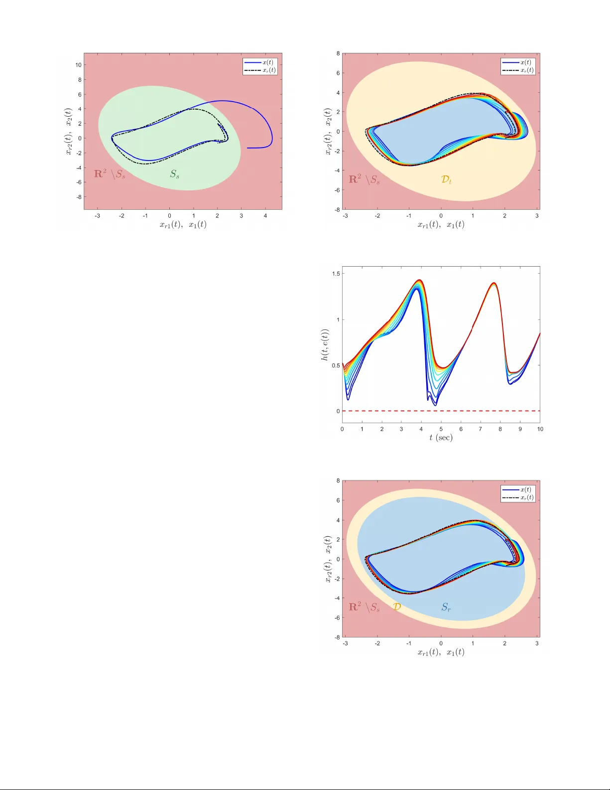
Safety-Critical Adaptiv e Contr ol with Nonlinear Refer ence Model Systems Ehsan Arabi Kunal Gar g Dimitra Panagou Abstract — In this paper , a model refer ence adaptive con- trol architecture is proposed for uncertain nonlinear systems to achieve pr escribed performance guarantees. Specifically , a general nonlinear reference model system is considered that captures an ideal and safe system beha vior . An adaptive control architectur e is then proposed to suppr ess the effects of system uncertainties without any prior knowledge of their magnitude and rate upper bounds. More importantly , the proposed control architectur e enforces the system state trajectories to evolve within a user-specified prescribed distance from the refer ence system trajectories, satisfying the safety constraints. This elim- inates the ad-hoc tuning pr ocess for the adaptation rate that is con ventionally required in model reference adaptive control to ensure safety . The efficacy of the proposed control architecture is also demonstrated through an illustrative numerical example. I . I N T RO D U C T I O N Adaptiv e control systems are control algorithms that miti- gate the effects of system uncertainties and exogenous distur - bances. Ho wev er , one of the limiting factors of these control systems is their lack of verifiable system performance. Model reference adaptiv e control generally consists of a reference model system and a control architecture along with an update law . In the design of the update law , the choice of the adaptation rate plays a crucial role in the overall system performance and in how much the system trajectories deviate from the reference model trajectories (i.e., from the ideal system behavior). As a result, the ad-hoc tuning process of the adaptation rate that is essential for safety-critical applications for keeping the system trajectories within the safe set, usually relies heavily on excessiv e vehicle testing and hence is time-consuming and costly . T o address this challenge, model reference adaptiv e con- trol algorithms are proposed to achieve strict performance guarantees in [ 1 – 6 ]. Similar to most of model reference adaptiv e control literature, the reference model systems in these studies follow linear dynamics. Ho wev er , nonlinear reference systems are preferable for several practical applica- tions, especially for those in volving guidance and control of highly-maneuverable aircraft, guided projectiles, and space Ehsan Arabi is a Postdoctoral Research Fellow of the Department of Aerospace Engineering at the University of Michigan, Ann Arbor , MI 48109, USA (email: earabi@umich.edu ). Kunal Garg is a Ph.D. Candidate of the Department of Aerospace Engineering at the Univ ersity of Michigan, Ann Arbor, MI 48109, USA (email: kgarg@umich.edu ). Dimitra P anagou is an Assistant Professor of the Department of Aerospace Engineering and the Director of the Distributed Aerospace Systems and Control Laboratory at University of Michigan, Ann Arbor, MI 48109, USA (email: dpanagou@umich.edu ). The authors would like to acknowledge the support of the Air Force Office of Scientific Research under aw ard number F A9550-17-1-0284. launch vehicles. Notable contributions to the adapti ve control literature using nonlinear reference systems are documented by the authors of [ 7 – 13 ]. In particular , [ 7 ] proposes an adaptiv e control algorithm for scalar nonlinear systems based on a nonlinear reference system, while [ 8 ] extends this result for a general class of uncertain nonlinear systems. In [ 9 ], the L 1 adaptiv e control method is used with nonlinear reference models. A sliding mode control design is proposed in [ 10 ] using the state-dependent Riccati equation. Furthermore, ap- plications of adapti ve control with nonlinear reference model systems in acti ve steering systems, tail-controlled missiles, and satellite attitude control are studied respectiv ely in [ 11 ], [ 12 ] and [ 13 ]. Y et, the aforementioned approaches do not establish any strict performance guarantees on the system trajectories, and they may violate the safety requirements specially during the transient time. Therefore, in safety- critical applications, a control designer either requires a- priori and almost complete knowledge of upper and lower bounds on the system uncertainties, or need to perform an ad-hoc tuning process for rendering the closed-loop system trajectories within the safe set (see [ 3 ] and references therein for more details). Our contrib ution is to present and analyze a ne w model reference adapti ve control architecture based on nonlinear reference models, with strict performance guarantees. Specif- ically , the proposed control architecture suppresses effects of system uncertainties independently of their magnitude and rate upper bounds, and enforces the system state trajectories to ev olve within a user-specified prescribed distance from the reference system states, satisfying the system safety constraints. For the case when the reference trajectories are av ailable prior to implementation, a time-varying perfor- mance bound is imposed on the system error vector . When the av ailable information is limited to a set of reference sys- tem trajectories, a constant performance bound is imposed, which is characterized based on the minimum distance of the reference set and the boundary of the safe set. This result can be viewed as a generalization of the results in [ 3 , 4 ] where a set-theoretic model reference adaptive control is proposed for linear dynamical systems with linear reference models. In fact, the presented results in this paper reduce to the control algorithms in [ 3 , 4 ] for a special case (see Remark 4 ). An illustrative numerical example is also provided to demonstrate the efficac y of the proposed architectures. I I . M A T H E M A T I C A L P R E L I M I N A R I E S W e be gin with the notation used in this paper . R , R n , and R n × m respectiv ely denote the set of real numbers, the set of n × 1 real column vectors, and the set of n × m real matrices; R + (resp., R + ) and R n × n + denote the set of positiv e real numbers (resp., non-negati ve reals) and the set of n × n positiv e-definite real matrices; D n × n denotes the set of n × n diagonal matrices, bd ( S ) denotes the boundary of the set S ⊂ R n , and “ , ” denotes equality by definition. In addition, we use ( · ) T to denote the transpose operator , ( · ) − 1 to denote the in verse operator , det( · ) to denote the determinant operator, k · k to denote the Euclidean norm, k · k F to denote the Frobenius norm, λ min ( A ) (resp., λ max ( A ) ) to denote the minimum (resp., maximum) eigen v alue of the square matrix A , dist ( A, B ) = inf x ∈ A,y ∈ B k x − y k to denote the distance between the sets A, B ⊂ R n , and dist ( x, B ) = inf y ∈ B k x − y k to denote the distance of x ∈ R n from the set B ⊂ R n . The gradient of a continuously differentiable function f : R n → R m , ev aluated at x ∈ R n is denoted as ∇ f ( x ) , ∂ f ∂ x ( x ) . Next, we introduce the definition of the projection op- erator . Let Ω be a con vex h ypercube in R n defined as Ω =  θ ∈ R n : ( θ min i ≤ θ i ≤ θ max i ) i =1 , 2 , ··· ,n  , where ( θ min i , θ max i ) denote the minimum and maximum bounds for the i th component of the n -dimensional parameter vector θ . Furthermore, let Ω ν be the second hypercube defined as Ω ν =  θ ∈ R n : ( θ min i + ν ≤ θ i ≤ θ max i − ν ) i =1 , 2 , ··· ,n  , where Ω ν ⊂ Ω for a sufficiently small positiv e constant ν . Definition 1 ([ 14 , 15 ]) . F or y ∈ R n , the pr ojection operator Pro j : R n × R n → R n is defined (componentwise) as Pro j( θ , y ) ,  [ θ max i − θ i ] /ν  y i when θ i > θ max i − ν and y i > 0 , Pro j( θ , y ) ,  [ θ i − θ min i ] /ν  y i when θ i < θ min i + ν and y i < 0 , and Pro j( θ , y ) , y i otherwise. It follows from Definition 1 that  θ − θ ∗  T  Pro j ( θ , y ) − y  ≤ 0 , θ ∗ ∈ Ω ν , where this inequality can be read- ily generalized to matrices using Pro j m (Θ , Y ) =  Pro j( col 1 (Θ) , col 1 ( Y )) , . . . , Pro j(col m (Θ) , col m ( Y ))  with Θ ∈ R n × m , Y ∈ R n × m , and col i ( · ) denoting i th column opera- tor . I I I . P RO B L E M F O R M U L A T I O N In this paper, we consider the class of uncertain nonlinear dynamical systems of the form ˙ x ( t ) = F ( x ( t )) + Gu ( t ) + D δ ( t, x ( t )) , x (0) = x 0 , (1) where x ∈ R n is the system state vector , F : R n → R n is a known system vector field with F (0) = 0 , G ∈ R n × m is an unknown control input matrix, u ( t ) ∈ R m is the control input, D ∈ R n × m is a known matrix, and δ : R + × R n → R m denotes system uncertainties. Let S s ⊂ R n denote the safe set of system states such that x ( t ) ∈ S s ensures safety . Consider the nonlinear reference model dynamics capturing an ideal (and safe) system behavior giv en by ˙ x r ( t ) = F r ( x r ( t ) , c ( t )) , x r (0) = x r0 , (2) where x r ∈ S r ⊂ S s is the reference system state vector , c ( · ) is a bounded command signal, and F r : R n × R → R n is the reference system vector field. The control objective is to design an adaptive control signal u ( · ) for the uncertain Fig. 1. Graphical representation of the sets S s and S r , and the performance bounds  ( t ) and  . nonlinear dynamical system in ( 1 ) to suppress the effects of system uncertainties such that the system state x ( · ) tracks the reference system state x r ( · ) while maintaining safety , i.e. x ( t ) ∈ S s , ∀ t ≥ 0 . Define the error vector between the system state tra- jectories and the reference system trajectories as e ( t ) , x ( t ) − x r ( t ) . If e ( t ) ∈ D t where D t , { e : k e k <  ( t ) } with the time-varying performance bound  ( t ) , dist ( x r ( t ) , R n \ S s ) ∈ R + , then x ( t ) ∈ S s , i.e., the trajectories of the uncertain dynamical system remain within the safe set S s (see Figure 1 ). In other words, if the control architecture limits the maximum deviation of the system state trajectories from the reference system by the performance bound  ( t ) , that is k e ( t ) k ≤  ( t ) for all t ≥ 0 , then safety is guaranteed (see Remark 5 for case with a constant performance bound ¯  ). This is a challenging task since the calculated upper bound on the system error signal in standard adapti ve control designs is generally conservati ve, and depends on the upper bounds of system uncertainties [ 3 ]. W e now introduce a standard assumption on system uncertainty parameterization [ 14 , 16 , 17 ]. Assumption 1. The system uncertainty given by ( 1 ) is parameterized as δ ( t, x ( t )) = W T p ( t ) σ p ( x ( t )) , (3) wher e W p ( t ) ∈ R s × m is a bounded time-varying unknown weight matrix with a bounded time rate of change (i.e., k W p ( t ) k F ≤ w p and k ˙ W p ( t ) k F ≤ w pd for some unknown w p , w pd ∈ R + ) and σ p : R n → R s is a known basis function of the form σ p ( x ) = [ σ p1 ( x ) , σ p2 ( x ) , . . . , σ p s ( x )] T . Assumption 2. The unknown contr ol input matrix G in ( 1 ) is parameterized as G = D Λ , (4) wher e Λ ∈ R m × m + ∩ D m × m is a bounded unknown contr ol effectiveness matrix. Remark 1. The pr esented r esults in this paper can be r eadily extended to the class of nonlinear systems with state- dependent contr ol matrix, i.e., G = G ( x ( t )) in ( 1 ) , wher e G ( x ( t )) = D Λ H ( x ( t )) and det( H ( x ( t )) 6 = 0 hold [ 8 , 18 ]. Using ( 1 ) and ( 2 ) along with Assumptions 1 and 2 , the system error dynamics can be written as ˙ e ( t ) = F ( x ( t )) − F r ( x r ( t ) , c ( t )) + D Λ  u ( t ) +Λ − 1 W T p ( t ) σ p ( x ( t ))  , e (0) = e 0 , (5) with e 0 , x 0 − x r0 . In the absence of system uncertainties (i.e., δ ( t, x ( t )) ≡ 0 and Λ = I m × m ), one can write ( 5 ) as ˙ e ( t ) = F ( x ( t )) − F r ( x r ( t ) , c ( t )) + D u n , (6) where u n = u n ( x ( t ) , x r ( t ) , c ( t )) ∈ R m is a nominal control law . Assumption 3. In the absence of system uncertainties (i.e., δ ( t, x ( t )) ≡ 0 and Λ = I m × m ), there exist a nominal control law u n = u n ( x ( t ) , x r ( t ) , c ( t )) ∈ R m such that the origin of the system err or dynamics in ( 6 ) is exponentially stable with a continuously differ entiable positive definite function V : D t → R , D t ⊂ S s satisfying k 1 k e ( t ) k 2 ≤ V ( e ( t )) ≤ k 2 k e ( t ) k 2 , (7) ∀ e ( t ) ∈ D t and its time derivative satisfying ˙ V ( e ( t )) = ∇ V T ( e ( t )) g ( e ( t )) ≤ − M ( e ( t )) , (8) k 0 k e ( t ) k 2 ≤ M ( e ( t )) , (9) wher e ∇ V ( e ( t )) = ∂ V ( e ( t )) /∂ e ( t ) , g ( e ( t )) = F ( x ( t )) − F r ( x r ( t ) , c ( t )) + D u n ( x ( t ) , x r ( t ) , c ( t )) and k 0 , k 1 and k 2 ar e positive constants. Remark 2. The nominal control input u n satisfying Assump- tion 3 can be found by various methods for some special classes of system: if ( 1 ) and ( 2 ) are linear , then the LQR contr ol input satisfies this assumption (see Remark 4 ); if the said systems ar e polynomial, then sum-of-squares (SOS) techniques can be used to find the nominal contr oller (see [ 19 , 20 ] and refer ences therein); or , a QP based method [ 21 ] can be used to compute a contr ol input for a larg er class of nonlinear , contr ol affine systems. Remark 3. Let h ( t, e ( t )) , k 1  2 ( t ) − V ( e ( t )) . If h ( t, e ( t )) > 0 , ∀ t ≥ 0 , then e ( t ) ∈ D t , ∀ t ≥ 0 . Assumption 4. The time derivative of  ( t ) e xists, and satisfies the condition | ˙  | ≤ α 1 2  if ˙  < 0 , wher e α 1 = k 0 k 2 , for all t ≥ 0 . Note that Assumption 4 limits the rate of change in the performance bound  ( t ) only when this bound is decreasing. More importantly , since this bound is characterized based on the safe set S s and the reference system trajectories x r ( t ) where x r ( t ) ∈ S s , ∀ t ≥ 0 , one can alw ays find a performance bound  ( t ) such that it satisfies Assumption 4 . I V . A DA P T I V E C O N T R O L A R C H I T E C T U R E W I T H P E R F O R M A N C E G UA R A N T E E S In this section, we design and analyze an adaptive control architecture for enforcing a performance bound on the system error v ector, limiting the de viation of system trajectories from the reference model trajectories. T o this end, we rewrite ( 5 ) as ˙ e ( t ) = F ( x ( t )) − F r ( x r ( t ) , c ( t )) + D u n ( x ( t ) , x r ( t ) , c ( t )) + D Λ  u ( t ) + Λ − 1 W T p ( t ) σ p ( x ( t )) − Λ − 1 u n ( x ( t ) , x r ( t ) , c ( t ))  , e (0) = e 0 . (10) Defining W ( t ) = [Λ − 1 W T p ( t ) , − Λ − 1 ] T ∈ R ( s + m ) × m and σ ( x ( t ) , x r ( t ) , c ( t )) = [ σ T p ( x ( t )) , u T n ( x ( t ) , x r ( t ) , c ( t ))] T ∈ R ( s + m ) , ( 10 ) can be expressed as ˙ e ( t ) = g ( e ( t )) + D Λ  u ( t ) + W T ( t ) σ ( · )  . (11) Note that k W ( t ) k F ≤ w and k ˙ W ( t ) k F ≤ w d automatically holds, for some unknown w , w d ∈ R + as a direct conse- quence of Assumption 1 . Motiv ated by the structure of the system error dynamics in ( 11 ), let the adaptive control law be u ( t ) = − ˆ W T ( t ) σ ( · ) , (12) where ˆ W ∈ R ( s + m ) × m is an estimate of the unkno wn weight matrix W satisfying the parameter adjustment mechanism ˙ ˆ W ( t ) = γ Pro j m  ˆ W ( t ) , h ( t, e ) + V ( e ) h 2 ( t, e ) σ ( · ) ∇ V T ( e ) D  , ˆ W (0) = ˆ W 0 , (13) with γ ∈ R + being a constant adaptation rate and ˆ W max being the projection operator bound. For the next theorem presenting the main result of this paper , we now write the system error dynamics and the weight estimation error dynamics respectively as ˙ e ( t ) = g ( e ( t )) − D Λ ˜ W T ( t ) σ ( · )  , e (0) = e 0 , (14) ˙ ˜ W ( t ) = γ Pro j m  ˆ W ( t ) , h ( t, e ) + V ( e ) h 2 ( t, e ) σ ( · ) ∇ V T ( e ) D  − ˙ W ( t ) , ˜ W (0) = ˜ W 0 , (15) where ˜ W ( t ) , ˆ W ( t ) − W ( t ) is the weight estimation error . Theorem 1. Consider the uncertain nonlinear dynamical system given by ( 1 ) subject to Assumptions 1 - 3 , the nonlinear r eference model given by ( 2 ) capturing an ideal system behavior , and the feedback contr ol law given by ( 12 ) along with ( 13 ). If e 0 ∈ D t , then the closed-loop dynamical system trajectories given by ( 14 ) and ( 15 ) are bounded, and e ( t ) ∈ D t ∀ t ≥ 0 , i.e., the system state vector x ( t ) r emains within the safe set S s for all times. Due to page limitations, the proof of the above theorem will be reported elsewhere. Here, we only provide a sketch of the proof. Specifically , consider the energy function Ψ : D t × R ( s + m ) × m → R + giv en by Ψ( e, ˜ W ) = V ( e ) h ( t, e ) + γ − 1 2 tr  ( ˜ W ( t )Λ 1 / 2 ) T ( ˜ W ( t )Λ 1 / 2 )  . (16) The time deri vativ e of ( 16 ) along the closed-loop system trajectories ( 14 ) and ( 15 ) can be written as ˙ Ψ  e, ˜ W  ≤ − α 1 Ψ  e, ˜ W  + α 2 − α 1  V ( e ) h ( t, e )  2 − 2 k 1  ( t ) ˙  ( t ) V ( e ) h 2 ( t, e ) , (17) where α 1 , k 0 /k 2 ∈ R + and α 2 , d + α 1 γ − 1 ˜ w k Λ k / 2 ∈ R + . If ˙  ( t ) ≤ 0 and V ( e ) < 2 k 1  ( t ) | ˙  ( t ) | /α 1 hold, it follows from definition of h ( t, e ) and Assumption 4 that h ( t, e ) > k 1  2 ( t ) − 2 k 1  ( t ) | ˙  ( t ) | α 1 > 0 . (18) Thus, the closed-loop system trajectories giv en by ( 14 ) and ( 15 ) are bounded and e ( t ) ∈ D t . If the above conditions for ˙  ( t ) and V ( e ) do not hold, one can write ˙ Ψ  e, ˜ W  ≤ − α 1 Ψ  e, ˜ W  + α 2 . (19) It now follows that the energy function Ψ  e, ˜ W  is upper bounded by Ψ  e, ˜ W  ≤ Ψ max , where Ψ max , max { Ψ 0 , α 2 /α 1 } ∈ R + , Ψ 0 , Ψ( e (0) , ˜ W (0)) ∈ R + , re- sulting in boundedness of the closed-loop system trajectories giv en by ( 14 ) and ( 15 ). Furthermore, using ( 16 ) one can write V ( e ) h ( t,e ) ≤ Ψ max . Hence, per Remark 3 , h ( t, e ( t )) > 0 , or equiv alently , e ( t ) ∈ D t for all t ≥ 0 , i.e., the system state x ( t ) remains within the safe set S s at all times. Remark 4. Considering a linear system dynamics and a linear refer ence dynamics respectively as ˙ x ( t ) = Ax ( t ) + B Λ( u ( t ) + δ ( t, x ( t ))) , (20) ˙ x r ( t ) = A r x r ( t ) + B r c ( t ) , (21) Assumption 3 is equivalent to the existence of the contr ol gains K 1 ∈ R m × n and K 2 ∈ R m × n c known as matc hing conditions such that A r = A − B K 1 and B r = B K 2 hold [ 14 , 22 ]. In this special case, define the weighted Euclidean norm of system err or as || e ( t ) || P = p e T ( t ) P e ( t ) wher e P ∈ R n × n + is a solution to the Lyapuno v equation 0 = A T r P + P A r + R , R ∈ R n × n + . By choosing V ( e ( t )) = || e ( t ) || 2 P , the update law in ( 13 ) r educes to ˙ ˆ W ( t ) = 2 γ Pro j m  ˆ W ( t ) , σ ( · ) k 1  2 ( t ) e T ( t ) P B ( k 1  2 ( t ) − || e ( t ) || 2 P ) 2  , (22) with ˆ W (0) = ˆ W 0 , which is in the same form as the proposed update law in [ 3 , 4 ] for the set-theoretic model r eference adaptive contr ol using general ized restricted potential func- tions (see (5) and (6) of [ 4 ]). Remark 5. If it is desir ed to work with constant performance bound instead of the time-varying performance bound dis- cussed in this section, one can define ¯  , inf t ≥ 0  ( t ) and consider the time-in variant set ¯ D , { e ( t ) | k e ( t ) k ≤ ¯  } instead of D t . In addition, consider the case when only a set of refer ence system trajectories is available for contr ol design instead of the r efer ence system tr ajectories prior to implementation. In this case, x r ( t ) ∈ S r for all t ≥ 0 , for some S r ⊂ S s ; hence, one can define a time-in variant performance bound as ¯  , dist ( S r , R n \ S s ) ∈ R + with the set ¯ D defined similarly as above (see Figur e 1 ). V . I L L U S T R A T I V E N U M E R I C A L E X A M P L E In this section, we present a numerical example to demon- strate the ef ficacy of the proposed control architecture. Specifically , we consider the uncertain dynamical system giv en by ˙ x ( t ) = F ( x ( t )) + D Λ u ( t ) + D δ ( t, x ( t )) , x (0) = x 0 , with F ( x ( t )) =  x 2 ( t ) − x 1 ( t ) − x 1 ( t ) x 2 ( t ) + x 2 2 ( t )  , D =  0 1  , where x ( t ) = [ x 1 ( t ) , x 2 ( t )] T ∈ R 2 denotes the system state vector . In addition, the unknown system un- certainty has the form δ ( t, x ( t )) = 0 . 3 sin(0 . 1 t ) x 1 ( t ) + 0 . 3 cos(0 . 3 t ) x 1 ( t ) x 2 ( t ) + x 1 ( t ) x 2 2 ( t ) . W e next consider the nonlinear reference model representing the forced V an der Pol oscillator [ 8 , 23 ] given by  ˙ x r1 ( t ) ˙ x r2 ( t )  =  x r2 ( t ) − x r1 ( t ) + µx r2 ( t )(1 − x 2 r1 ( t )) + c ( t )  , (23) with x r (0) = x r0 and c ( t ) = 1 . 2 sin( t ) . In the absence of system uncertainties (i.e., δ ( t, x ( t )) ≡ 0 and Λ = 1 ), the nominal controller u n ( x ( t ) , x r ( t ) , c ( t )) = − l 1 e 1 ( t ) − l 2 e 2 ( t ) + x 1 ( t ) x 2 ( t ) − x 2 2 ( t ) + c ( t ) + µx r2 ( t )(1 − x 2 r1 ( t )) , with l 1 , l 2 ∈ R + , satisfies Assumption 3 , resulting in the exponentially stable error dynamics ˙ e ( t ) = A e e ( t ) , e (0) = e 0 with A e =  0 1 − (1 + l 1 ) − l 2  , and the L yapunov function V ( e ( t )) = e T ( t ) P e ( t ) where P ∈ R 2 × 2 + is a solution to the L yapunov equation 0 = A T e P + P A e + R , R ∈ R 2 × 2 + . W e set the initial conditions to x 0 = x r0 = [2 , 2] T , µ = 1 , l 1 = l 2 = 3 , and the control ef fectiveness to Λ = 0 . 75 . In addition, the safe set for system trajectories is chosen as S s = { x ( t ) : x T ( t ) P x ( t ) < 3 . 2 } . Figures 2 and 3 present the performance of the nominal controller in the presence of system uncertainties. It is evident that the nominal controller is not capable of keeping the system state trajectories within the safe set S s . W e now consider two cases to illustrate how the proposed results with constant and time-varying performance bounds are used. First, we consider that the reference system trajectories x r ( t ) is kno wn prior to the implementation. In this case, the safety margin can be characterized as a time-varying set D t , and the time-v arying performance bound  ( t ) is selected based on the distance of the reference system trajectories from the safe set S s defined abo ve at each time instance. W e 0 1 2 3 4 5 6 7 8 9 10 -2 0 2 4 0 1 2 3 4 5 6 7 8 9 10 -2 0 2 4 0 1 2 3 4 5 6 7 8 9 10 -20 -10 0 Fig. 2. System performance with the nominal controller . Fig. 3. System state phase portrait with the nominal controller . apply the adaptive control signal in ( 12 ) with the proposed update law in ( 13 ) with different values of the adaptation rate γ ∈ [0 . 05 , 5] . Figure 4 shows that although with lower adaptation rates system state gets closer to the boundaries of the safe set S s , they nev er leave this set. This is also clear from Figure 5 where h ( t, e ( t )) is always positive resulting in e ( t ) ∈ D t ∀ t ≥ 0 . This sho ws that the obtained performance guarantee is independent of the selection of the adaptation rate γ as expected. W e now consider that only a set of reference system trajectories S r is known, where the safety mar gin can be characterized as a constant set D . Based on the selected reference model, the reference set S r is selected as S r = { x r ( t ) : x T r ( t ) P x r ( t ) < 2 . 8 } , where in this case the constant performance bound is selected as ¯  = 1 . 3 to ensure safety . W e now apply the adaptiv e control signal in ( 12 ) with the proposed update law in ( 13 ) with dif ferent values of the adaptation rate γ ∈ [0 . 05 , 5] . Figure 6 shows that the proposed controller ensures safety of the system state trajectories where the obtained performance guarantee is independent of the selection of the adaptation rate γ . This is also clear from Figure 5 where h ( e ( t )) is always positiv e resulting in e ( t ) ∈ D ∀ t ≥ 0 . Finally , Figures 8 and 9 compare the tracking performance for the proposed control architecture with constant and time-varying performance bounds. As expected, although a constant performance bound results in closer tracking of the reference trajectories, the control input is larger than the case with time-varying performance bound. In addition, one can see from Figure 9 that the time-varying perfor- mance bound results in lo wer effecti ve adaptation rate (i.e., γ ( h ( · ) + V ( · )) /h 2 ( · ) in ( 13 )), improving the robustness of the system. V I . C O N C L U S I O N In this paper , we developed a new model reference adap- tiv e control architecture based on nonlinear reference models for uncertain nonlinear systems. Specifically , the key feature of the proposed approach was to suppress the effects of system uncertainties reg ardless of their magnitude and rate Fig. 4. System state phase portrait with the proposed adaptive control architecture with time-varying performance bound for γ ∈ [0 . 05 , 5] (blue to red). Fig. 5. The e volution of h ( e ( t )) with the proposed adaptive control architecture with time-varying performance bound for γ ∈ [0 . 05 , 5] (blue to red). Fig. 6. System state phase portrait with the proposed adaptive control architecture with constant performance bound for γ ∈ [0 . 05 , 5] (blue to red). upper bounds. As a result, the system trajectories evolv e within a user-specified prescribed distance from the nonlinear reference trajectories. Based on the safety specifications for a gi ven system, this user-specified distance can be charac- terized to render the closed-loop system trajectories within 0 1 2 3 4 5 6 7 8 9 10 -0.05 0 0.05 0.1 0.15 0.2 0.25 0.3 0.35 Fig. 7. The e volution of h ( e ( t )) with the proposed adaptive control architecture with constant performance bound for γ ∈ [0 . 05 , 5] (blue to red). Fig. 8. Comparison of the tracking performance using the proposed adaptiv e control architecture with constant and time-varying performance bounds. Fig. 9. Comparison of the control signal (top) and effectiv e adaptation rate (bottom) using the proposed adaptiv e control architecture with constant and time-varying performance bounds. the safe set, without the requirement of an ad-hoc tuning process for the adaptation rate. An illustrative numerical example were further provided to demonstrate the ef ficacy of the proposed approach. R E F E R E N C E S [1] T . Y ucelen and J. S. Shamma, “ Adaptive architectures for distributed control of modular systems, ” American Control Confer ence , 2014. [2] J. A. Muse, “ A method for enforcing state constraints in adaptive control, ” in AIAA Guidance, Navigation and Control Conference , 2011. [3] E. Arabi, B. C. Gruenwald, T . Y ucelen, and N. T . Nguyen, “ A set- theoretic model reference adaptiv e control architecture for disturbance rejection and uncertainty suppression with strict performance guaran- tees, ” International Journal of Contr ol , vol. 91, no. 5, pp. 1195–1208, 2018. [4] E. Arabi and T . Y ucelen, “Set-theoretic model reference adaptive control with time-varying performance bounds, ” International Journal of Control , vol. 92, no. 11, pp. 2509–2520, 2019. [5] A. L ’Afflitto and T . A. Blackford, “Constrained dynamical systems, robust model reference adaptiv e control, and unreliable reference signals, ” International Journal of Control , 2018. [6] A. LAfflitto, “Barrier L yapunov functions and constrained model reference adapti ve control, ” IEEE Contr ol Systems Letters , vol. 2, no. 3, pp. 441–446, 2018. [7] D. J. W agg, “ Adaptive control of nonlinear dynamical systems using a model reference approach, ” Meccanica , vol. 38, no. 2, pp. 227–238, 2003. [8] T . Y ucelen, B. Gruenwald, J. A. Muse, and G. De La T orre, “ Adap- tiv e control with nonlinear reference systems, ” in American Control Confer ence , 2015. [9] X. W ang and N. Hovakimyan, “ L 1 adaptiv e controller for nonlinear time-varying reference systems, ” Systems & Contr ol Letters , vol. 61, no. 4, pp. 455–463, 2012. [10] F . Kara and M. U. Salamci, “Model reference adaptive sliding sur- face design for nonlinear systems, ” IEEE T ransactions on Industry Applications , vol. 54, no. 1, pp. 611–624, 2017. [11] Y . Kawaguchi, H. Eguchi, T . Fukao, and K. Osuka, “Passi vity-based adaptiv e nonlinear control for acti ve steering, ” IEEE International Confer ence on Contr ol Applications , pp. 214–219, 2007. [12] F . Peter, M. Leit ˜ ao, and F . Holzapfel, “ Adaptive augmentation of a new baseline control architecture for tail-controlled missiles using a nonlinear reference model, ” in AIAA Guidance, Navigation, and Contr ol Confer ence , 2012. [13] S. Scarritt, “Nonlinear model reference adaptive control for satellite attitude tracking, ” in AIAA Guidance, Navigation and Contr ol Confer - ence and Exhibit , 2008. [14] E. Lavretsky and K. Wise, Robust and Adaptive Control with Aer ospace Applications . Springer Science & Business Media, 2012. [15] J.-B. Pomet and L. Praly , “ Adaptive nonlinear regulation: Estimation from the L yapunov equation, ” IEEE T ransactions on Automatic Con- tr ol , vol. 37, no. 6, pp. 729–740, 1992. [16] K. S. Narendra and A. M. Annaswamy , Stable Adaptive Systems . Courier Corporation, 2012. [17] P . A. Ioannou and J. Sun, Robust Adaptive Contr ol . Courier Corporation, 2012. [18] K. Y . V olyanskyy , W . M. Haddad, and A. J. Calise, “ A new neuroad- aptiv e control architecture for nonlinear uncertain dynamical systems: Beyond σ - and e -modifications, ” IEEE T ransactions on Neural Net- works , vol. 20, no. 11, pp. 1707–1723, 2009. [19] Q. Zheng, “Sum of squares based nonlinear control design techniques, ” Ph.D. dissertation, North Carolina State University , 2009. [20] M. M. Peet, “Exponentially stable nonlinear systems hav e polynomial L yapunov functions on bounded regions, ” IEEE T ransactions on Automatic Contr ol , vol. 54, no. 5, pp. 979–987, 2009. [21] A. D. Ames, X. Xu, J. W . Grizzle, and P . T abuada, “Control barrier function based quadratic programs for safety critical systems, ” IEEE T ransactions on Automatic Contr ol , vol. 62, no. 8, pp. 3861–3876, 2016. [22] N. T . Nguyen, Model-Reference Adaptive Contr ol: A Primer . Springer , 2018. [23] W . M. Haddad and V . Chellaboina, Nonlinear Dynamical Systems and Contr ol: A Lyapunov-based Approac h . Princeton University Press, 2008.