math.OC 2021-06-07 0

Learning How to Dynamically Route Autonomous Vehicles on Shared Roads

Road congestion induces significant costs across the world, and road network disturbances, such as traffic accidents, can cause highly congested traffic patterns. If a planner had control over the routing of all vehicles in the network, they could ea…

Authors: Daniel A. Lazar, Erdem B{i}y{i}k, Dorsa Sadigh

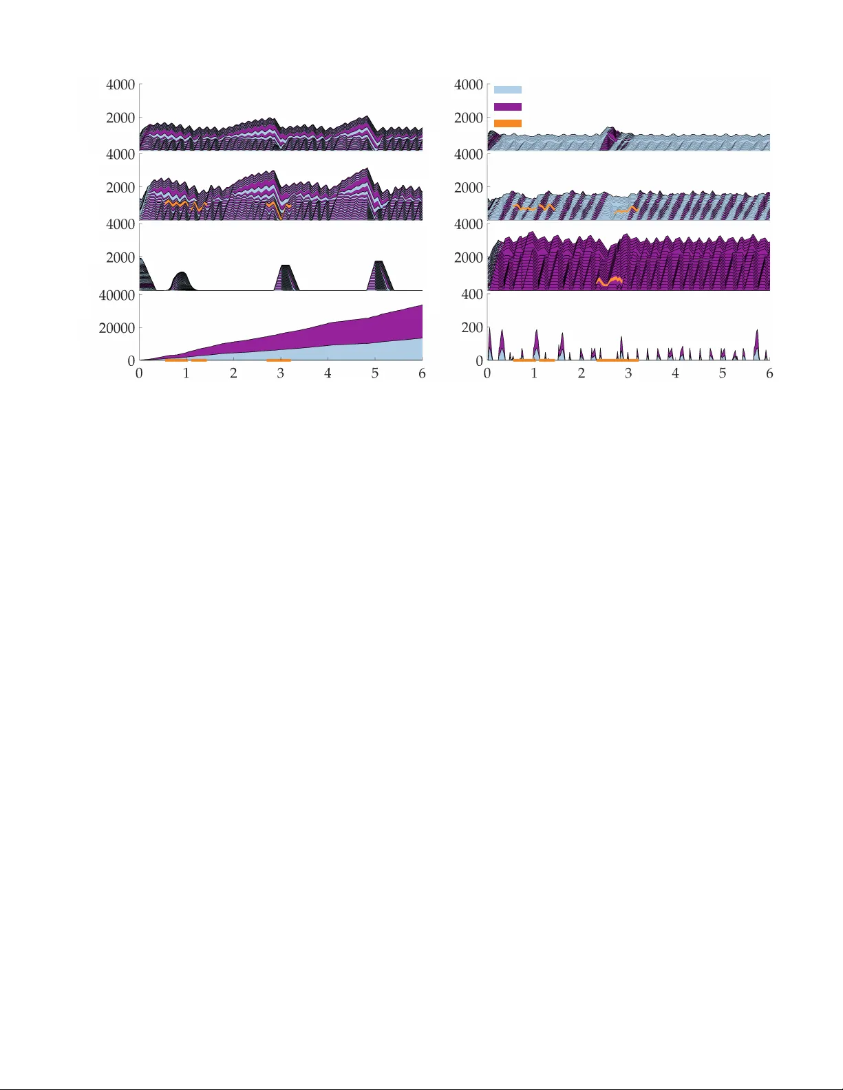
Learning How to Dynamically Route Autonomous Vehicles on Shared Roads

Lear ning How to Dynamically Route A utonomous V ehicles on Shar ed Roads Daniel A. Lazar ∗ , Erdem Bıyık ∗ , Dorsa Sadigh, Ramtin Pedarsani Abstract —Road congestion induces signiﬁcant costs acr oss the world, and road network disturbances, such as trafﬁc accidents, can cause highly congested trafﬁc patterns. If a planner had control over the routing of all vehicles in the netw ork, they could easily re verse this effect. In a more realistic scenario, we consider a planner that controls autonomous cars, which are a fraction of all present cars. W e study a dynamic routing game, in which the r oute choices of autonomous cars can be controlled and the human drivers react selﬁshly and dynamically . As the problem is prohibiti vely large, we use deep reinfor cement learning to learn a policy f or controlling the autonomous vehicles. This policy indirectly inﬂuences human drivers to route themselves in such a way that minimizes congestion on the network. T o gauge the effectiveness of our learned policies, we establish theoretical results characterizing equilibria and empirically com- pare the learned policy results with best possible equilibria. W e pro ve properties of equilibria on parallel roads and provide a polynomial-time optimization f or computing the most efﬁcient equilibrium. Moreov er , we show that in the absence of these policies, high demand and network perturbations would result in large congestion, whereas using the policy greatly decreases the travel times by minimizing the congestion. T o the best of our knowledge, this is the ﬁrst work that employs deep reinfor cement learning to reduce congestion by indirectly inﬂuencing humans’ routing decisions in mixed-autonomy trafﬁc. Keyw ords —Dynamic routing, reinf orcement learning, mixed- autonomy trafﬁc I . I N T RO D U C T I O N C ONGESTION can result in substantial economic and social costs [1] which have only been gro wing in recent years, especially with the advent of ride-hailing services [2, 3]. Congestion is formed by a number of mechanisms, such as when many vehicles try to enter a road at the same time. A higher -lev el cause is from ho w people choose their routes – when people selﬁshly choose the quickest routes av ailable to them, this often results in greater congestion and longer trav el time than if people had their routes chosen for them optimally in terms of the ov erall experienced delay [4]. There are some existing methods for ﬁghting congestion, such as congestion pricing [5], v ariable speed limits [6] and highway ramp metering [7]. Howe ver , they can be difﬁcult to administer, and can require signiﬁcant changes to infrastructure. The introduction of autonomous vehicles to public roads provides an opportunity for better congestion management [8]. Our key idea is that by controlling the routing of autonomous v ehicles, we can change the delay associated with trav ersing each road, thereby indirectly inﬂuencing peoples’ routing choices. By inﬂuencing people to use more “socially ∗ Authors contributed equally . Daniel Lazar is with the Department of Electrical and Computer Engineering, UC Santa Barbara dlazar@ece.ucsb.edu Erdem Bıyık is with the Department of Electrical Engineering, Stanford Univ ersity ebiyik@stanford.edu Dorsa Sadigh is with the Departments of Computer Science and Electrical Engineering, Stanford Univ ersity dorsa@cs.stanford.edu Ramtin Pedarsani is with the Department of Electrical and Computer Engineering, UC Santa Barbara ramtin@ece.ucsb.edu advantageous” routes, we can eliminate long queues and signiﬁcantly reduce trafﬁc jams on roads. The model for mixed-autonomy trafﬁc, meaning trafﬁc with both human-dri ven and autonomous vehicles, is comple x, in volving very large and continuous state space and continuous action space. Having human drivers dynamically respond to the choices of the autonomous vehicles further complicates the matter , making a dynamic programming-based approach and other classical methods infeasible. Because of this, we use model-free deep reinforcement learning (RL) to learn a policy without requiring access to the dynamics of the transportation network. Speciﬁcally , we show it is possible to learn a policy via proximal policy optimization (PPO) [9] that mitigates trafﬁc congestion by managing routing of autonomous cars given the network state. T o understand the performance of the learned policy , we in vestigate the equilibrium beha vior of the network. Previous works [10, 11] have shown that there is a wide spectrum of equilibria in traf ﬁc networks, meaning situations in which ev eryone is taking the quickest route immediately av ailable to them, and these equilibria can have greatly varying av erage user delay . W e establish efﬁcient ways to compute equilibria in the network and compare the best equilibrium (in terms of latency) with the RL policy , which works regardless of whether equilibrium conditions hold or not. W e sho w that the learned policy reaches the ‘desirable’ equilibria that have lo w trav el times when starting with v arying trafﬁc patterns, and can reco ver network functionality after a disturbance such as a traf ﬁc accident. T o summarize, our contributions are as follo ws: • Theor etical analysis: W e characterize equilibria in the network and deriv e a polynomial-time computation for ﬁnding optimal equilibria of parallel networks. • F inding a contr ol policy via deep RL: W e employ deep RL methods to learn a routing policy for autonomous cars that effecti vely sav es the trafﬁc network from unboundedly large delays. W e show via simulation that the RL policy is able to bring our network to the best possible equilibrium when starting from a congested state or after a network disturbance on parallel networks. W e further sho w that an MPC-based approach and a greedy optimization method fail to do so, and thus is outperformed by the RL-based method in general networks. W e visualize our framework in the schematic diagram Fig. 1. Literature re view . Many works seek to understand how much trafﬁc network latency could be improved if vehicle routing was controlled by a central planner , including works on congestion games [4, 12 – 15]. Some study ho w indirectly inﬂuencing peoples’ routing choices by providing them net- work state information af fects network performance [16, 17]. Stack elberg Routing , in which only some of the vehicles are controlled, is another way to inﬂuence routing [18, 19]; some works incorporate the dynamics of human routing choices [20]. Fig. 1: The schematic diagram of our framew ork. Our deep RL agent processes the state of the traf ﬁc and outputs a control policy for autonomous cars’ routing. While providing useful techniques for analysis, the congestion game frame work does not reﬂect a fundamental empirical understanding about vehicle ﬂo w on roads, namely that roads with low v ehicle density ha ve a roughly constant latency , and roads with high density see latenc y increase as ﬂo w decreases . W orks on CTM [21, 22] capture this phenomenon, including works that characterize equilibria on roads described with CTM [7]. Notably , some consider equilibria of parallel-path Stackelber g Games, including with mixed autonomy [10, 11]. Howe ver , their analyses are limited to steady-state and do not capture the dynamics. [23] considers a Fundamental Diagram of T rafﬁc-based model for slowly v arying traf ﬁc. They formulate this as a Stackelber g Game and design routing information for users to minimize overall latency and bound the resulting inefﬁcienc y in a simple network. Howe ver , they only consider a single-vehicle type, not a mix ed-autonomy setting. Some works look at the lo w-level control of autonomous cars, speciﬁcally controlling acceleration to smooth ﬂow and ease congestion at bottlenecks [24–26]; [27] provides a benchmark for gauging the performance of these techniques. Other works learn ramp metering policies [28], localize congestion [29], and model lane-change behavior with a neural netw ork [30]. In addition to these learning methods, there has also been an effort to use RL for route selection [31] and dri ver choice modeling in trafﬁc assignment problem [32 – 35]. Again using RL, [36] shows re ward shaping mechanisms could be utilized to reach better equilibria. Recently , [37, 38] dev elop a hierarchical approach to optimize fares, tolling and signal control in the high-le vel whereas a multi-agent RL method models the driv ers in the lower le vel. Although these works show the effecti veness and potential of RL methods in transportation, to the best of our kno wledge, these methods have not been used in a routing game with mixed-autonomy trafﬁc where a central planner aims to reduce congestion by indirectly inﬂuencing humans’ routing via the routing of autonomous vehicles. W ithout any reinforcement learning component, some w orks provide macroscopic models of roads shared between human- dri ven and autonomous cars. [39] models highway bottlenecks in the presence of platoons of autonomous vehicles mixed in with human-driven vehicles. The authors relate their model to a CTM type-model similar to the model presented belo w , though it is speciﬁc to a single highway . [40] describes a microscopic model to determine the effect of autonomy on throughput, yielding fundamental diagrams. The fundamental relationship between autonomy le vel and critical density in our model mirrors that of [41], which de velops a CTM model for mixed autonomy traf ﬁc. Some works solv e the dynamic trafﬁc assignment problem for networks with a CTM-based ﬂo w model, including some which decompose the optimization to enable optimizing ﬂow on large networks [42]. In contrast, our works studies the setting in which some ﬂo w demand is controlled to optimize the system performance, and some ﬂow demand updates according to a selﬁsh update rule. This precludes the use of such decomposition techniques, since the optimization can no longer be formulated as a linear program. Because of this, we use RL to solve for a routing policy in our setting. I I . V E H I C L E FL O W DY N A M I C S : M O D E L I N G R OA D S In this section we describe dynamics go verning ho w vehicle ﬂow travels on a road. W e extend the CTM, a widely used model that discretizes roads into cells , each with uniform density [21, 22], for mixed-autonomy trafﬁc. In CTM, each road segment has a maximum ﬂow that can traverse it. The key idea of our extension is that since autonomous vehicles can keep a shorter headway (distance to the car in front of it), the greater the fraction of autonomous vehicles on a road, the greater the maximum ﬂow that the road can serve [11]. Accordingly , our extension of CTM lies in the dependence of cell parameters on the autonomy level , or the fraction of autonomous vehicles, in each cell. W e use our capacity model in conjunction with Daganzo’ s CTM formulation in [21, 43], the combination of which we describe in the following. W e consider a network of roads with a single origin and destination for all vehicles in the network. The origin and destination are connected by the set of simple paths P . Each path is composed of a number of cells, and we denote the set of cells composing path p by I p . W e generally use i and p as indices for cells and paths, respectiv ely . In the CTM, ev ery cell has a critical density , and when the density of a cell exceeds the critical density , that cell is congested . W e model the critical density as being dependent on the autonomy le vel. This is because autonomous v ehicles maintain a different nominal headway than human-dri ven vehicles; in other words, autonomous vehicles may require more space in front of them due to prediction error , or less space, as they may react faster than human dri vers. Accordingly , we use the model in [44] to model the capacity of a cell. Using this model, each cell i has a free-ﬂow velocity , ¯ v i , as well as a nominal headway for vehicles trav eling at the free-ﬂo w velocity — h h i cells/vehicle for human-driven vehicles and h a i for autonomous vehicles. The capacity of the cell then Fig. 2: (a) Fundamental diagram of trafﬁc governing vehicle ﬂow in each cell of the Cell Transmission Model. The solid line corresponds to a cell with only human-driven vehicles; the dashed line represents a cell with both vehicle types at autonomy level α i . Green and red respectiv ely represent a cell in free-ﬂow and congestion. (b) The ﬂow from one cell to another is a function of the density n and autonomy lev el α in each cell. In both ﬁgures, we suppress the notation for path p . v aries with the autonomy le vel, denoted α i ∈ [0 , 1] . W e use b i to denote the number of lanes in a cell. W e model vehicles as slowing down when the headway experienced decreases below the nominal headway required and accordingly model the critical density as follows, as in [11, 15, 44, 45]: ˜ n i ( α i ) := b i / ( α i h a i + (1 − α i ) h h i ) . (1) Each cell also has a vehicle density , n i = n h i + n a i , where n h i and n a i are, respecti vely , the number of human-dri ven and autonomous vehicles. Thus, α i = n a i / ( n h i + n a i ) . As the cells are very large compared to the vehicles, we consider these quantities to be continuous variables. As mentioned above, CTM has two regimes for v ehicle ﬂow: free-ﬂo w , when cell density is less than the critical density , and congestion, when cell density is greater than the critical density but less than the jam density ¯ n i , the density at which ﬂow stops completely . Three factors limit the ﬂow from one cell to another . One is the capacity , or maximum ﬂo w out of a cell, which is the ﬂow of vehicles that trav erse the cell at the critical density: ¯ F i ( α i ) := ¯ v i ˜ n i ( α i ) . (2) The ﬂow out of a cell is limited by the sending function of that cell, which is the minimum of the capacity of the cell and the demand of vehicles in the cell: S i ( α i ( k )) = min( ¯ F i ( α i ) , ¯ v i n i ( k )) . The ﬂo w entering a cell is limited by that cell’ s recei ving function, which is the minimum of its capacity and its supply of vehicles: R i ( α i ( k )) = min( ¯ F i ( α i ) , ( ¯ n i − n i ) w i ( α i )) , where w i is the shockwave speed , the speed at which slo wing wav es of traf ﬁc propagate upstream: w i ( α i ) := ¯ v i ˜ n i ( α i ) / ( ¯ n i − ˜ n i ( α i )) . In the following, we use f i ( k ) to denote the ﬂo w out of cell i at time k and y i ( k ) to denote the ﬂow into cell i . W e use the standard superscripts for human- driv en and autonomous ﬂow , with the relationships f h i ( k ) + f a i ( k ) = f i ( k ) and y h i ( k ) + y a i ( k ) = y i ( k ) . Accordingly , n h i ( k + 1) = n h i ( k ) + y h i ( k ) − f h i ( k ) , n a i ( k + 1) = n a i ( k ) + y a i ( k ) − f h i ( k ) . (3) Since some cells might be a part of more than one path, we also track the paths of the human-dri ven and autonomous vehicles in each cell. W e use µ h i ( p, k ) and µ a i ( p, k ) to denote the fraction of human-driv en and autonomous vehicles, respectiv ely , in cell i at time k that are taking path p . If cell i is not on path p , let µ h i ( p, k ) = µ a i ( p, k ) = 0 . Extending the dev elopment in [46], we formulate a calcula- tion of the ﬂo w of mix ed autonomous vehicles through general junctions. W e deﬁne O as the set of intersections, or junctions, in the network. W e use Ξ( o ) to denote the set of turning mov ements through intersection o , with a turning mo vement denoted by a tuple, such as [ i, o, j ] ∈ Ξ( o ) , where i denotes the incoming cell, and j denotes the outgoing cell. As before, we consider all cells to hav e one direction of travel. F or intersection o we deﬁne a set of conﬂict points C ( o ) , and Ξ( c ) denotes the set of turning movements through the intersection which pass through conﬂict point c , where c ∈ C ( o ) . These routes may hav e different priority le vels, so for each [ i, o, j ] ∈ Ξ( c ) we deﬁne β c ioj > 0 as the priority of turning movement [ i, o, j ] through conﬂict point c . Each conﬂict point has some supply R c , which we assume is independent of the level of autonomy of the vehicles passing through it. The relativ e priority of the turning mov ements will determine the relative ﬂow of each turning movement through the conﬂict point. In a slight abuse of notation, we use f ioj ( k ) to denote the total ﬂow of v ehicles through turning mov ement [ i, o, j ] at time k ; we use f h ioj ( k ) and f a ioj ( k ) to denote the ﬂow of human and autonomous vehicles, respecti vely , through the turning mo vement. W e use Γ( o ) and Γ − 1 ( o ) to denote the set of cells exiting and entering junction o , respectiv ely . W e then calculate the ﬂo ws at each time step as in Algorithm 1. An interpretation of this algorithm is as follo ws. The set A denotes the set of turning movements with ﬂows that can yet be increased, and each turning mov ement is assigned a rate at which its ﬂo w increases. As sending and receiving limits are reached, turning mo vements are remov ed from A until there are no more turning mov ements left to increase. In more concrete terms, ﬁrst calculate the fraction of vehicles in each incoming cell which are headed to each outgoing cell. Then initialize all ﬂo ws to 0 and initialized the unused sending and recei ving capacity for each cell and conﬂict point. W e then ﬁnd relati ve rates of ﬂow increase, δ ioj , for the turning mov ements. In the loop, we calculate the similar rates of ﬂo w increases for the recei ving cells and conﬂict points based on the rates previously found. Then, the ﬂows are increased by the established rates until either a sending limit, a cell receiving limit, or conﬂict point capacity is reached. Any turning movement that has reached its sending limit is removed from the set of turning movements with further ﬂow increases, A . Similarly , any turning movement that exits from a cell which has reached its receiving limit is remov ed from A , and the same with turning mo vements through conﬂict points which hav e reached their capacity . The loop repeats until A is empty . Having calculated the ﬂo w through the intersection, the states Algorithm 1 Flow Calculation 1: procedure F L O W C A L C U L A T I O N ( Intersection o ) 2: ∀ [ i, o, j ] ∈ Ξ( o ) , p h ioj ← X p ∈P : i,j ∈I p µ h i ( p, k ) p a ioj ← X p ∈P : i,j ∈I p µ a i ( p, k ) p ioj ← n h i ( k ) p h ioj + n a i ( k ) p a ioj n h i ( k ) + n a i ( k ) 3: ∀ [ i, o, j ] ∈ Ξ( o ) , f ioj ← 0 f h ioj ← 0 f a ioj ← 0 ˜ S ioj ← S i ( α i ( k )) p ioj ∀ ( o, j ) ∈ Γ( o ) , ˜ R oj ← R j ( α j ( k )) ∀ c ∈ C ( o ) , ˜ R c ← R c 4: For all [ i, o, j ] ∈ Ξ( o ) , set δ ioj such that ∀ [ i, o, j ] ∈ Ξ( o ) , ∀ [ i 0 , o, j 0 ] ∈ Ξ( o ) , δ ioj δ i 0 oj 0 = p ioj p i 0 oj 0 , where i can equal i 0 and j can equal j 0 , and ∀ c ∈ C ( o ); ∀ [ i, o, j ] ∈ Ξ( c ) ∀ [ i 0 , o, j 0 ] ∈ Ξ( c ) , δ ioj δ i 0 oj 0 = β c ioj p ioj β c i 0 oj 0 p i 0 oj 0 , where i can equal i 0 and j can equal j 0 . 5: A ← Ξ( o ) 6: while A 6 = ∅ do 7: ∀ ( o, j ) ∈ Γ( o ) , δ oj ← X [ i,o,j ] ∈ A p ioj ∀ c ∈ C ( o ) , δ c ← X [ i,o,j ] ∈ Ξ( c ) ∩ A p ioj 8: θ = min { min [ i,o,j ] ∈ A ˜ S ioj δ ioj , min ( o,j ) ∈ Γ( o ) ,δ oj > 0 ˜ R oj δ oj , min c ∈ C ( o ): δ c > 0 ˜ R c δ c } 9: ∀ [ i, o, j ] ∈ A, f ioj ← f ioj + θ δ ioj f h ioj ← f h ioj + θ δ ioj (1 − α i ( k )) f a ioj ← f a ioj + θ δ ioj α i ( k ) ˜ S ioj ← ˜ S ioj − θ δ ioj ∀ ( oj ) ∈ Γ( o ) , ˜ R oj ← ˜ R oj − θ δ oj ∀ c ∈ C ( o ) , ˜ R c ← ˜ R c − θ δ oj 10: A ← A \ { [ i, o, j ] ∈ A : ˜ S ioj = 0 } A ← A \ { [ i, o, j 0 ] ∈ A : ˜ R oj = 0 ∧ p ioj 0 > 0 } A ← A \ { [ i, o, j ] ∈ c : ˜ R c = 0 ∀ c ∈ C ( o ) } 11: end while 12: retur n f ioj , f h ioj , f a ioj , ∀ [ i, o, j ] ∈ Ξ( o ) 13: end procedure of each cell is updated as follows. W e compute the incoming ﬂows for the outgoing cells as follows: ∀ ( o, j ) ∈ Γ( o ) , y h j ( k ) = X [ i,o,j ] ∈ Ξ( o ) f h ioj y a j ( k ) = X [ i,o,j ] ∈ Ξ( o ) f a ioj y j ( k ) = y h j ( k ) + y a j ( k ) (4) T o calculate the outgoing ﬂows of the incoming cells, ∀ ( i, o ) ∈ Γ − 1 ( o ) , f h i ( k ) = X [ i,o,j ] ∈ Ξ( o ) f h ioj f a i ( k ) = X [ i,o,j ] ∈ Ξ( o ) f a ioj f i ( k ) = f h i ( k ) + f a i ( k ) , (5) where Γ − 1 ( o ) denotes the set of cells going into intersection o . (3) updates the human-driven and autonomous vehicle densities of each cell at the next time step. T o update the fraction of vehicles in the outgoing cells on each path, ∀ ( o, j ) ∈ Γ( o ) , µ h j ( p, k + 1) = P [ i 0 ,o,j ] ∈ Ξ( o ) f h i ( k ) µ h i ( p, k ) + µ h j ( p, k )( n h j ( k ) − f h j ( k )) n h j ( k + 1) , µ a j ( p, k + 1) = P [ i 0 ,o,j ] ∈ Ξ( o ) f a i ( k ) µ a i ( p, k ) + µ a j ( p, k )( n a j ( k ) − f a j ( k )) n a j ( k + 1) . Accidents. T o ev aluate the performance of the de veloped RL policy in reacting to disturbances, we consider stochastic accidents occuring in the network, each of which causes one lane to be closed. W e let accidents occur in any cell at any time with equal probability as long as the jam density does not decrease belo w the current density of the cell. Each accident is cleared out after some number of time steps, drawn from a Poisson distribution. If ¯ b i lanes of cell i are closed due to accidents, then the jam density and the critical density for the cell reduce to ( b i − ¯ b i ) /b i of their original values. Thus, accidents introduce time-dependency to these v ariables. I I I . N E T W O R K DY N A M I C S : R O U T I N G F O R H U M A N S A N D AU T O N O M O U S V E H I C L E S As mentioned abov e, we consider a network with a set of possible paths P . W e use λ h and λ a to denote the human-driv en and autonomous vehicle demands, respecti vely . W e model all vehicles entering the network as entering a queue , a single cell with inﬁnite capacity . W e use 0 for the index of this cell. The routing choices of autonomous vehicles leaving the queue is determined by the central controller , and the routing choices of human-dri ven vehicles lea ving it are determined from the latencies associated with each path, detailed below . A. Human choice dynamics In general, people wish to minimize the amount of time spent traveling. Ho wever , people do not change routing choices instantaneously in response to ne w information; rather they hav e some inertia and only change strategies sporadically . Moreov er , we assume people only account for current conditions and do not strategize based on predictions of the future [47]. Accordingly , we use an evolutionary dynamic to describe how a population of users choose their routes. 1 Speciﬁcally , we model the human driver population as follo wing Hedge Dynamics, also called Log-linear Learning [48 – 50]. Let ( µ h 0 ( p, k )) p ∈P represent the initial routing of human- dri ven vehicles at time k ; accordingly , P p ∈P µ h 0 ( p, k ) = 1 for all k . Humans will update their routes based on their estimates of ho w long it will take to trav erse each path. Howe ver , it is not always possible to predict travel time accurately on general networks, since vehicles entering later on a dif ferent path may inﬂuence the trav el time of vehicles entering earlier . Because of this, we consider that humans ha ve an estimate ˆ ` p ( k ) of the true latency ` p ( k ) . W ith these estimates, the routing vector is updated as follows. µ h 0 ( p, k + 1) = µ h 0 ( p, k ) exp( − η h ( k ) ˆ ` p ( k )) P p 0 ∈P µ h 0 ( p 0 , k ) exp( − η h ( k ) ˆ ` p 0 ( k )) . (6) The ratio of the volume of vehicles using a path at successiv e time steps is in versely proportional to the exponential of the delay experienced by users of that path. The learning rate η h ( k ) may be decreasing or constant. Krichene et al. introduce this model in the context of humans’ routing choices and simulate a congestion game with Amazon Mechanical T urk users to show the model accurately predicts human behavior [51]. W e note that though we use this speciﬁc model for human choice for our simulations, the control method described later does not require this speciﬁc choice of human choice model. Our theoretical analysis similarly is not restricted to this choice of dynamics and works for any human choice model in which all ﬁxed points of the dynamics satisfy human selﬁshness. B. Autonomous vehicle contr ol policy W e assume that we hav e control ov er the routing of autonomous vehicles. W e justify this by en visioning a future in which autonomous vehicles are of fered as a service rather than a consumer product. W e then assume that a city can coordinate with the owner of an autonomous ﬂeet to decrease congestion in the city . Moreov er , unlike traditional tolling, coordination between autonomous vehicles and city infrastructure allows for fast-changing and geographically ﬁnely quantized tolls, enabling routing control to be achiev ed through incentiv es [52, 53]. The initial routing of autonomous vehicles is then our control parameter by which we inﬂuence the state of trafﬁc on the network. Consistent with the previous notation, we denote the initial autonomous routing as ( µ a 0 ( p, k )) p ∈P ∈ R |P | ≥ 0 , where P p ∈P µ a 0 ( p, k ) = 1 . W e assume the existence of a central controller , or social planner , which dictates µ a 0 by processing the state of the network. At each time step, we let the controller observe: • the number of human-driven and autonomous vehicles in each cell and in the queue, 1 Alternately , one could model individual users as learning agents, posing it as a Multi-Agent Reinforcement Learning problem. Howe ver , we consider large networks with too many human agents for this to be feasible. • binary states for each lane that indicates whether the lane is closed due to an accident or not. W e use deep RL to arriv e at a policy for the social planner to control the autonomous v ehicle routing, µ a 0 . Since the state space is very lar ge and both state and action spaces are continuous, a dynamic programming-based approach is infeasible. For instance, ev en if we discretized the spaces, say with 10 quantization lev els, and did not hav e accidents, we would hav e 10 82 possible states and 10 actions for a moderate- size network with only 2 paths and 40 cells in total. W e wish to minimize the total latency experienced by users, which is equal to summing o ver time the number of users in the system at each time step. Accordingly , the stage cost is: J ( k ) = X i ∈I n i ( k ) . (7) Due to their high performance in continuous control tasks [9, 54], we employ policy gradient methods to learn a policy that produces µ a 0 giv en the observations. Speciﬁcally , we use state- of-the-art PPO with an objective function augmented by adding an entropy bonus for suf ﬁcient exploration [9, 55]. W e b uild a deep neural network, and train it using Adam optimizer [56]. An ov erview of the PPO method and the set of parameters we use are presented in the appendix (Sec. VII-C and Sec. VII-D ). Each episode has a ﬁxed number of time steps. In order to e valuate the performance of our control policy , we use three criteria. The ﬁrst is the throughput of the network – we wish to hav e a polic y that can serve any feasible demand, thereby stabilizing the queue. The second is the average delay experienced by users of the network, which we measure by counting the number of vehicles in the system. The third is the con ver gence to some steady state; we wish to av oid wild oscillations in congestion. T o contextualize the performance of our control policy in this frame work, we ﬁrst establish the performance of equilibria of the network. I V . E Q U I L I B R I U M A N A L Y S I S In this section, we examine the possible equilibria of our dynamical system, which characterize the possible steady state behaviors of the system. A network with a gi ven demand can have a variety of equilibria with varying average user delay . If our control achieves overall delay equal to that of the best possible equilibrium, it is a successful policy . Section V sho ws empirically that our learned polic y can achiev e the best equilibrium in a variety of settings. In this section, we ﬁrst formulate an optimization which solves for the most efﬁcient equilibrium, which is computation- ally hard. Motiv ated by this, we restrict the class of networks considered and prove theoretical properties of this restricted class. Using these properties, we formulate a ne w optimization formulation to solve for the most efﬁcient equilibrium and prov e it is solvable in polynomial time. A. Equilibrium F ormulation W e deﬁne two notions of equilibrium: one related to the vehicle ﬂow dynamics, and one related to human choice dynamics. 2 Deﬁnition 1 (Path Equilibrium) . W e deﬁne a path equilibrium for path p as a set of cell densities ( n h i ( k ) , n a i ( k )) i ∈I p that, for a given constant ﬂow entering the ﬁrst cell on the path, y h i ( k ) and y a i ( k ) , the cell densities ar e constant. Deﬁnition 2 (Network Equilibrium) . W e deﬁne a network equilibrium as a set of cell densities ( n h i ( k ) , n a i ( k )) i ∈I and human vehicle routing ( µ h 0 ( p, k )) p ∈P , such that for a given constant entering ﬂow y h 0 ( k ) and y a 0 ( k ) and a given constant autonomous vehicle r outing ( µ a 0 ( p, k )) p ∈P , the human vehicle r outing, subject to the dynamics in (6) , is constant. W e are interested in satisfying both notions of equilibrium – both the path equilibrium, which deals with the vehicle ﬂo w dynamics, and the network equilibrium, which deals with the human choice dynamics. Accordingly , the pair can be considered a Stackelber g Equilibrium for a leader controlling the autonomous vehicles who wishes to maximize the social utility in the presence of selﬁsh human demand. W e formulate the following optimization to solve for the most efﬁcient equilibrium (satisfying both notions of equilibrium deﬁned abov e), i.e. the equilibrium which minimizes the total trav el time of all users of the network. W e drop all time indices since we consider quantities that are constant ov er time. min ( n h i ,n a i ,f h i ,f a i ,y h i ,y a i ,µ h i ( p ) ,µ a i ( p ) ,` p ) i ∈I ,p ∈P X i ∈I n i s.t. ∀ o ∈ O : procedur e F L O W C A L C U L A T I O N (Intersection o ) (4) , (5) ∀ i ∈ I : y h i = f h i , y a i = f a i , α i = n a i / ( n h i + n a i ) X i 0 ∈U i f h i 0 µ h i 0 ( p ) = f h i µ h i ( p ) , X i 0 ∈U i f a i 0 µ a i 0 ( p ) = f a i µ a i ( p ) ` p = X i ∈ p ( n h i + n a i ) / ( f h i + f a i ) ∀ p, p 0 ∈ P : µ h 0 ( p )( ` p − ` p 0 ) ≤ 0 While this formulation solves for the most efﬁcient equi- librium of an y traf ﬁc network, it is computationally dif ﬁcult, especially due to the ﬁnal constraint. Due to this, we introduce a restricted class of networks that we consider for the remainder of this section, which allo ws us to compute equilibria in polynomial time with respect to the number of paths. Deﬁnition 3 (Bottleneck) . W e deﬁne a bottleneck as a r egular junction at which the number of lanes decr eases, decr easing the capacity of the cells. Assumption 1. W e consider a par allel network in which leaving the ﬁrst cell, vehicles choose a path and paths do not shar e cells, meaning that each cell is identiﬁed with only one path, aside from the downstr eam-most cell which has inﬁnite capacity . W e further consider that all cells in the path 2 These deﬁne equilibria in the sense of dynamical systems, and do not strictly correspond to game-theoretic notions of equilibria. Under Assumption 3 below , the set of equilibria for the dynamics of human choice will correspond to the set of Nash Equilibria where the payoff is the path latency . have the same model parameters, except for a bottleneck after the m n p upstr eam-most cells. In other words, we consider a parallel network where each path is composed of identical cells except for a single junction with a decrease in the number of lanes. Fig. 1 shows an example of such a network. For ease of analysis, we ﬁrst establish properties of Path Equilibria, then Network Equilibria. B. P ath equilibrium As mentioned above, we restrict our considered class of paths to those with a single bottleneck, meaning one point on the path at which cell capacity drops. Formally , we consider each path p to hav e m n p cells, each with b n p lanes, followed by m b p cells downstream, each with b b p lanes, where b b p < b n p . W e deﬁne r p := b b p /b n p ∈ (0 , 1) . In a slight abuse of notation, we use the subscript p for parameters that are constant over a path under Assumption 1, and the superscript n for cells before the bottleneck and b for the bottleneck and cells do wnstream of it. W e now present a theoretical result that completely analytically characterizes the path latencies that can occur at equilibrium. Theorem 1. Under Assumption 1 a path p with ﬂow dynamics described in Section II that is at P ath Equilibrium will have the same autonomy level in all cells. Denote this autonomy level α p . If the vehicle ﬂow demand is strictly less than the minimum cell capacity , the path will have no congested cells. Otherwise, the path will have one of the following latencies, wher e γ p ∈ { 0 , 1 , 2 , . . . , m n p } : ` p = |I p | ¯ v p + γ p (1 − r p ) ¯ n n p ( α p h a p + (1 − α p ) h h p ) r p ¯ v p b n p . Pr oof. The proof is composed of three lemmas. W e ﬁrst establish a property of path equilibria that allows us to treat the vehicle ﬂo w as if it were composed of a single car type. With this, we use the CTM to characterize possible equilibria on a path. W e then deriv e the delay associated with each congested cell. Combining the latter two lemmas yields the theorem. Lemma 1. A path in equilibrium with nonzer o incoming ﬂow has the same autonomy level in all cells of the path, whic h is equal to the autonomy level of the vehicle ﬂow onto the path. F ormally , a path p with demand ( ¯ λ h p , ¯ λ a p ) in equilibrium has, for all cells i in I p , α i = ¯ λ a p / ( ¯ λ h p + ¯ λ a p ) . W e defer the proof of the lemma to the appendix. W ith this, our path equilibria analysis simpliﬁes to that of single-typed traf ﬁc, with the autonomy level treated as a variable parameter . The next lemma, similarly to Theorem 4.1 of [7], completely characterizes the congestion patterns that can occur in cell equilibria. For this lemma, we consider the cell indices in a path to be increasing, where the cell immediately do wnstream from a cell i has index i + 1 . Lemma 2. Under Assumption 1, if the demand on a path is less than the minimum capacity of its cells, they will be uncongested at path equilibrium. Otherwise, a path with demand equal to the minimum cell capacity will have m n p possible path equilibria, corr esponding to one of the following sets of congested cells, wher e j is the index of the m n p th cell:  ∅ , { j } , { j − 1 , j } , . . . , { j − m n p + 1 , . . . , j − 2 , j − 1 , j }  . Pr oof. As mentioned abov e, this lemma relates closely to Theorem 4.1 of [7]. Ho wever , we cannot directly apply that theorem due to differing assumptions; namely they assume ¯ F i +1 = ( ¯ n i − ˜ n i ) w i for all i . W e therefore offer a similar proof, tailored to our assumptions. For ease of notation, we drop all path subscripts p as well as the cell index for the free-ﬂow velocity parameter ¯ v . In light of Lemma 1, we also suppress the autonomy level ar guments to capacity ¯ F i and critical density ˜ n i . The ﬂow equation then becomes f i = min( ¯ v n i , ( ¯ n i +1 − n i +1 ) w i +1 , ¯ F i , ¯ F i +1 ) . W e begin by proving that if the vehicle ﬂow demand is strictly less than the minimum capacity , i.e. the bottleneck capacity , then the only equilibrium has no congested cells. Let us use j 0 to denote the index of the ﬁnal cell in the path. Under Assumption 1 there is no supply limit to the ﬂow exiting a path, so f j 0 = min( ¯ v n j 0 , ¯ F j 0 ) . Since f 0 = f j 0 < ¯ F j 0 , f 0 = f j 0 = ¯ v n j 0 . The deﬁnition of capacity , ¯ F i = ¯ v ˜ n i , then implies that n j 0 < ˜ n j 0 , meaning that cell j 0 is uncongested, so ¯ v n j 0 < ( ¯ n j 0 − n j 0 ) w j 0 . This is the base case for a proof by induction. Consider cell i that is uncongested ( i.e. n i < ˜ n i ). Since by assumption all cells hav e ﬂow strictly less than the cell’ s capacity , f i = ¯ v n i < ¯ F i . Then consider the ﬂow entering cell i : f i − 1 = min( ¯ v n i − 1 , ( ¯ n i − n i ) w i , ¯ F i − 1 ) = f i < ¯ F i < ( ¯ n i − n i ) w i . The f act that ¯ F i ≤ ¯ F i − 1 then implies that f i − 1 = ¯ v n i − 1 , so cell i − 1 is uncongested, proving the lemma’ s ﬁrst statement. The second statement assumes the ﬂow on the path is equal to the minimum capacity . The cells in the bottleneck segment all hav e the same capacity , which we denote ¯ F b ; this capacity is less than the capacity of the cells in the nonbottleneck segment. This means all bottleneck cells will be operating at capacity (and therefore ha ve vehicle density equal to their critical density); ﬂow on the path is therefore equal to ¯ F b . W e now turn to the nonbottleneck segment. W e ﬁrst note that if a nonbottleneck cell is uncongested then the preceeding cell must be uncongested as well, using the same reasoning as that proving the ﬁrst statement abov e. Next, consider the ﬂow out of the downstream-most cell of the nonbottleneck segment: f j = min( ¯ v n j , ( ¯ n j +1 − n j +1 ) w j +1 , ¯ F j ) = ¯ F b < ¯ F j , so f j = min( ¯ v n j , ( ¯ n j +1 − n j +1 ) w j +1 ) . Cell j can be uncongested, in which case the cell density is such that ¯ v n j = ¯ F b , or the cell can be congested, in which case the second term dominates. Then, if nonbottleneck cell i is congested, the ﬂo w into it is f i − 1 = min( ¯ v n i − 1 , ( ¯ n i − n i ) w i ) . Again, to achie ve this ﬂow , cell i − 1 can be either congested or uncongested. As sho wn abov e, if uncongested, then all upstream cells must be uncongested as well, yielding the second statement in the lemma. W e use these properties to ﬁnd a closed-form expression for the latency incurred by traveling through a bottleneck cell, which when combined with Lemma 2, completes the proof. Lemma 3. The latency incurred by traveling thr ough a congested cell is as follows. 1 ¯ v p + (1 − r p ) ¯ n n p ( α p h a p + (1 − α p ) h h p ) r p ¯ v p b n p . Pr oof. Recall that we assume paths ha ve a uniform free- ﬂow velocity across all cells in a path, where path p has free-ﬂo w velocity ¯ v p . W e deﬁne [ m n p ] as the set of cells before the bottleneck, which ha ve b n p lanes. The remaining cells, with indices in the set I p \ [ m n p ] , hav e b b p lanes. Further recall the deﬁnition r p = b b p /b n p . Let ¯ F n p ( α p ) denote the capacity of the cells before the bottleneck of path p with autonomy le vel α p and let ¯ F b p ( α p ) be the same for the bottleneck cell. Note that ¯ F b p ( α p ) = r p ¯ F n p ( α p ) . Similarly , let w n p ( α p ) and w b p ( α p ) denote the shockwave speed for prebottleneck cells and bottleneck cell, respectiv ely , on path p with autonomy le vel α p , as with jam densities ¯ n n p and ¯ n b p and critical densities ˜ n n p ( α p ) and ˜ n b p ( α p ) . Lemma 2 establishes all possible combinations of congested cells that a path at equilibrium can e xperience. W e now in vestigate how much delay each conﬁguration induces on the path, parameterized by the autonomy lev el of the path. By Lemma 2 and the deﬁnitions of r and capacity (2), f p = ¯ F b p = r p ¯ F n p ( α p ) = r p w n p ( α p )( ¯ n n p − ˜ n n p ( α p )) . (8) Let n c p ( α p ) denote the vehicle density in a congested cell on path p , which we know must occur upstream of the bottleneck (Lemma 2). Then, the ﬂow entering a congested cell before the bottleneck is f p = w n p ( α p )( ¯ n n p − n c p ( α p )) . Equating this with (8), we ﬁnd n c p ( α p ) = (1 − r p ) ¯ n n p + r p ˜ n n p ( α p ) . T o use this to ﬁnd the latency incurred by tra veling through a congested cell, we divide the density by the ﬂow , as follows. n c p ( α p ) f p = n c p ( α p ) ¯ F b p ( α p ) = (1 − r p ) ¯ n n p + r p ˜ n n p ( α p ) r p ¯ v p ˜ n n p ( α p ) = 1 ¯ v p + (1 − r p ) ¯ n n p ( α p h a p + (1 − α p ) h h p ) r p ¯ v p b n p . T ogether , the lemmas prove the theorem. The two terms abov e are the free-ﬂo w delay and the per- cell latency due to congestion, respectiv ely . Theorem 1 allows us to calculate the possible latencies of a path as a function of its autonomy le vel α p . Since in a netw ork equilibrium all used paths have the same latency , we can calculate network equilibria more efﬁciently than comprehensiv ely searching over all possible routings. Howe ver , equilibria may not exist, e ven with a ﬁne time discretization – in equilibrium the path latencies must be equal, but by Theorem 1, road latenc y is a function of the integer γ p . T o av oid this artifact, when analyzing network equilibria we consider the cells to be small enough that we can consider the continuous variable γ p ∈ [0 , m n p ] . C. Network equilibrium W e deﬁne the best equilibrium to be the equilibrium that serves a giv en ﬂow demand with minimum latency . W e are no w ready to establish properties of network equilibria, as well as ho w to compute the best equilibria. W e use the follo wing two assumptions in our analysis of network equilibrium. Assumption 2. No two paths have the same fr ee-ﬂow latency . Assumption 3. The initial choice distribution has positive human-driven and autonomous vehicle ﬂow on each path. Note that the Assumption 2 is not strictly necessary but is useful for easing analysis. A similar analysis could be performed in its absence. W e justify Assumption 3 by noting that humans are not entirely rational and that our choice model does not capture all reasons a person may wish to choose a route, and some small fraction of people will choose routes that seem less advantageous at ﬁrst glance. Theorem 2. Under Assumptions 1 and 2, a r outing that minimizes total latency when all users (both human drivers and autonomous user s) ar e selﬁsh can be computed in O ( |P | 3 log |P | ) time. A r outing that minimizes total latency when human drivers are selﬁsh and autonomous users ar e contr olled can also be computed in O ( |P | 3 log |P | ) time. Pr oof. T o establish properties of network equilibria, we in- troduce some notation. W e use a p = |I p | / ¯ v p to denote the free-ﬂow latency of path p . W e also use P ≤ a p = { p 0 ∈ P : a p 0 ≤ a p } , which denotes the set of paths with free-ﬂow latenc y less than or equal to that of path p . W e similarly deﬁne the expression with other comparators, e .g. P a p . This proposition follows from Deﬁnition 2 and Assumption 3. The next lemma follo ws, with proof deferred to the appendix. Proposition 1. In a network equilibrium, 1) All paths with selﬁsh drivers have the same latency , and 2) All paths without selﬁsh drivers have equal or gr eater latency . Lemma 4. If the set of equilibria contains a r outing with positive ﬂow only on paths P ≤ a p , then ther e exists a r outing in the set of equilibria in which path p is in fr ee-ﬂow . Lemma 5. Under Assumption 2, if some users ar e selﬁsh and some users ar e not selﬁsh, then the best equilibrium will have the following pr operties: 1) the path with larg est fr ee-ﬂow latency used by selﬁsh users will be in fr ee-ﬂow , 2) all paths with lower fr ee-ﬂow latency will be congested, 3) paths with greater fr ee-ﬂow latency may have nonselﬁsh users, and 4) paths used with lar ger free-ﬂow latency that have nonselﬁsh users on them will be at capacity , except perhaps the path with lar gest fr ee-ﬂow latency used by nonselﬁsh users. Pr oof. Consider a network with some selﬁsh and some non- selﬁsh (controlled) users. Let p denote the path with the longest free-ﬂow latency that contains selﬁsh users. For the purpose of contradiction, let this path contain congested cells, and let this be the best equilibrium. Fix the nonselﬁsh ﬂow on all roads with longer free-ﬂow latency than p . By Lemma 4, there exists an equilibrium for the selﬁsh users in which p is in free-ﬂow . This results in less latency for the users on path p , and no selﬁsh user will ha ve greater delay (Proposition 1). This contradicts the premise, proving the ﬁrst property . The second property follows directly from Proposition 1 and Assumption 2. The third property follows from the deﬁnition of nonselﬁsh users, which can take a path with a lar ger latenc y than other av ailable paths. The best equilibrium minimized total latency . If there was a road with nonselﬁsh users that was not at capacity , while another path with higher latency has positi ve ﬂow , this would not be the best equilibrium, since a more ef ﬁcient routing would shift ﬂow from the higher latency path to the lower latency one. This yields the ﬁnal property . Using these properties, we prove Theorem 2. W e ﬁrst consider the setting in which all users are selﬁsh. W e use ` c p ( α p ) to denote the per-cell latency due to congestion, i.e. ` c p ( α p ) = (1 − r p ) ¯ n n p ( α p h a p +(1 − α p ) h h p ) r p ¯ v p b n p . Lemma 5 implies that for a gi ven demand, all equilibria in the set of most efﬁcient equilibria for that demand have one path that is in free-ﬂo w . W e can then formulate the search for a best equilibrium as an optimization. W e are helped by the fact that the best equilibria will use the minimum number of feasible paths, since all users experience the same delay . Then, for each candidate free-ﬂo w path (denote with index p 0 ), check feasibility of only using paths P ≤ a p 0 , and choose a routing that minimizes |P ≤ a p 0 | , i.e. the number of roads used. The reason for minimizing the number of used roads is that all users are experiencing the same latency (Proposition 1) and in the best equilibrium, the road with ﬂow on it that has longest free-ﬂow latency will be in free-ﬂow (Lemma 5). The feasibility can be checked as follows, with an optimization that utilizes Lemma 5. arg min ( f h p ,f a p ) p ∈P ≤ a p 0 , γ ∈ Q p ∈P a p 0 f a p a p s.t. X p ∈P ≤ a p 0 f h p = ¯ λ h , X p ∈P f a p = ¯ λ a f h p 0 + f a p 0 ≤ ¯ F p 0 ( f a p 0 f h p 0 + f a p 0 ) ∀ p ∈ P a p 0 : f a p ≤ ¯ F b (1) This can be reformulated as a linear program by the same mechanism. Again, we solve log |P | linear programs and choose the one corresponding to the minimum feasible p 0 . Using these properties to compute optimal equilibria, we establish a framew ork for understanding the performance of our learned control policy . If the policy can reach the best equilibrium latency starting from arbitrary path conditions we vie w the policy as successful. W e use this baseline to e valuate our experimental results in the follo wing section. A question then arises: if we have computed the best possible equilibria, why do we not directly implement that control? This approach is not fruitful, since the theoretical analysis of best equilibria giv es the control policy only in the steady state. In practice, the network can start in any state, including worse equilibria, from which good equilibria will not emerge when autonomous vehicles unilaterally use their routing in the best equilibrium. Besides, our equilibrium analysis is limited to parallel networks and extending it to more general networks would yield a nonconv ex optimization problem. A dynamic policy which depends on the current traf ﬁc state is therefore needed to guide the network to the best equilibrium. As shown in the follo wing section, the policy learned via deep reinforcement learning achiev es this guidance and reaches the best equilibrium in a variety of settings. V . E X P E R I M E N T S A N D R E S U LT S In all of the experiments 3 , we adopt the following parameters. All vehicles are 4 meters long. Human drivers keep a 2 second headway distance, whereas autonomous cars can keep 1 second. Each time step corresponds to 1 minute of real-life simulation. Each episode during deep RL training covers 5 hours of real- life simulation ( 300 time steps). In test time, we simulate 6 hours of real-life ( 360 time steps) to ensure the RL policy did not learn to minimize the latency in the ﬁrst 300 time steps and lea ve e xcess vehicles in the netw ork at the end. W e di vide paths into the cells such that it takes 1 time step to traverse each cell in free-ﬂow . W e initialize n i (0) ∼ unif (0 , 1 . 2 ˜ n i ) for all i ∈ I p for all p ∈ P . W e set the standard deviations of the zero-mean Gaussian demand noise to be ¯ λ h / 10 and ¯ λ a / 10 for human-driv en and autonomous vehicles, respectiv ely . Our overall control scheme can be seen in Fig. 1. As the learning model, we b uild a two-hidden-layer neural network, with each layer ha ving 256 nodes. W e train an RL agent for each conﬁguration that we will describe later on in simulated trafﬁc networks that are based on the mixed-autonomy trafﬁc 3 W e make the code available in the supplementary material. Fig. 3: The small general class network used for e xperiments. model and the dynamics that we described in Sections II and III. All trainings simulate 40 million time steps. 4 Depending on whether we ev aluate our RL-based approach with (or without) the accidents, we enable (or disable) accidents at the training phase. Howe ver , we note that the number of possible accident conﬁgurations in the network is far more than the expected number of accidents during all training episodes. Hence, successfully handling accidents requires good generalization performance. Similar to accidents, the demand distributions match between training and test en vironments. W e compare our method with two baselines: ﬁrst, a selﬁsh routing scheme, where all cars are selﬁsh and use the human choice dynamics presented in Sec. III-A , and second, a model predictiv e control ( MPC ) based controller which can perfectly simulate the network other than the uncertainty due to accidents and noisy demand. It plans for the receding horizon of 4 minutes and re-plans after ev ery 1 minute to minimize the number of cars in the network using a Quasi-Newton method (L-BFGS [57]). T o increase robustness against the uncertainty , it samples 12 different simulations of the network and tak es the average. W e note that this MPC can only be useful in small networks where some cars can enter the network and reach the destination within the MPC horizon of 4 minutes. While increasing the horizon may help MPC operate in larger networks, it causes a huge computational burden. In f act, even though we parallelized the controller ov er 12 Intel ® Xeon ® Gold 6244 CPUs (3.60 GHz), it took the controller 32 seconds on a verage to decide the routing of autonomous vehicles for the next 1 minute, which clearly indicates a practical problem. In all experiments, we set η h ( k ) (and η a ( k ) for the selﬁsh baseline) to be 0 . 5 for all k . A. General Class of Networks W e ﬁrst start by considering a small network of 9 cells and 7 junctions ( 1 regular junction, 3 merges and 3 div erges) as shown in Fig. 3, where the priority le vels of cells at mer ges are equal to their numbers of lanes. W e set the autonomy level of the demand ¯ α = 0 . 6 and the total demand ¯ λ h + ¯ λ a = 2 . 60 cars per second. W e set the probability of accidents such that the expected frequency of accidents is 1 per 100 minutes, and clearing out an accident takes 30 minutes on average [58]. For 4 Other hyperparameter values we use for PPO are in the Appendix. human choice dynamics, we assume humans’ latency estimates are based on the current states of each cell, i.e., they estimate the latencies as if the network is in steady-state. Fig. 4: Time vs. number of cars under selﬁsh, MPC and RL routing on the small general class network. Fig. 4 sho ws the number of cars in the network over time (mean ± standard error over 100 simulations). While MPC controller improv es over the selﬁsh routing, they both suf fer from linearly growing queues. On the other hand, RL controller stabilizes the queue and keeps the network uncongested. Fig. 5: OW network (adapted from [59]) used for e xperiments. Next, we consider a larger network sho wn in Fig. 5 as a graph where the numbers noted on the links denote the number of cells in that link in one direction. Each cell, excluding queues which has inﬁnite capacity , has 2 lanes. This is a quantized version of the OW network due to Ortúzar and W illumsen [59], and is widely used in the transportation literature [32, 36, 60, 61]. This is a lar ger network with 4 origin-destination pairs, 102 cells (and 2 queues) and 41 junctions ( 28 junctions with only one incoming and one outgoing cell, and 13 more general junctions). W e set the total demand to be ¯ λ h + ¯ λ a = 3 . 46 cars per second, distributed equally to the 4 origin-destination pairs in expectation. As there are 1752 possible different simple paths that vehicles could be taking, our action space is 1752 dimensional. While such an optimization is still possible with powerful computation resources, it might be unnecessary because an optimal solution is unlikely to utilize the paths that tra verse too many cells. W e therefore restrict our action space to the 10 shortest paths (with respect to the free-ﬂow latencies) between each origin and destination, and so adopt a 40 -dimensional action space. W e keep the other experiment parameters the same as the small network experiment above. Due to the network size and the computation cost to simulate the O W network, the MPC-based controller does not produce any useful results in a reasonable time as explained before. W e instead implemented the greedy optimization method of Krichene, Castillo, and Bayen [20] as a baseline. Speciﬁcally we used a genetic algorithm for the optimization with a constraint on the run time of one minute, as it is an online algorithm. It is important to note that RL policy makes a routing decision within a millisecond during test time. W e compare the RL controller with this greedy method and the selﬁsh routing. Fig. 6: T ime vs. number of cars under selﬁsh, greedy and RL routing on OW network. Fig. 6 sho ws the number of cars in the network over time (mean ± standard error ov er 100 simulations). Again, the selﬁsh routing and the greedy optimization method of [20] suffer from linearly growing queues, while RL controller is able to stabilize the queues and keeps the network uncongested ev en though the network may start from a congested state. Furthermore, we check whether the reduced action space is really suf ﬁcient. W e observe that, o ver 100 episodes, 98.92% of the autonomous vehicles were routed to the paths that are faster than the fastest path that is not in the action space. T o analyze the performance RL controller in comparison with the optimal equilibrium, we now move to parallel networks. B. P arallel Networks W e consider a parallel network from downto wn Los Angeles to the San Fernando V alle y with 3 paths. The highway numbers and the approximated parameter tuples (length, number of lanes, speed limit) are: 1) 110N (5 miles, 3 lanes, 60 mph); 101N (10 miles, 3 lanes for 5 miles then 2 lanes, 60 mph) 2) 10E (5 miles, 4 lanes, 75 mph); 5N (10 miles, 4 lanes, 75 mph); 134W (5 miles, 3 lanes, 75 mph) 3) 10W ; 405N (both 10 miles, 4 lanes, 75 mph); 101S (5 miles, 3 lanes, 75 mph) As the cells are now not shared between the paths, we employ better latency estimates for human choice dynamics: we compute them as the actual latencies that would occur if there were no accidents and no more demand into the network. W e perform 3 sets of experiments. In the ﬁrst two, we disable accidents and analyze the effects of varying the number of paths and autonomy . As the shortest path has 15 cells, we exclude MPC-based controller from our analysis as it is computationally prohibiti ve to adopt a receding horizon longer than 15 minutes. V arying number of paths. W e ﬁrst v ary the number of paths |P | ∈ { 2 , 3 , 4 } by duplicating, or removing, the third path. W e Fig. 7: V arying number of paths. (a) A verage number of cars in the system per episode during RL training. (b) T ime vs. number of cars in the system for the comparison of selﬁsh and RL routing in parallel networks. set the autonomy level of the demand ¯ α = 0 . 6 , and ¯ λ h + ¯ λ a to be 95% of the maximum capacity under this autonomy le vel. W e plot learning curves in Fig. 7 (a). It can be seen that ev en with |P | = 4 when observ ation space is 144 -dimensional, the agent successfully learns routing within 40 million time steps. W ith randomized initial states, the agents learn routing policies that achieve nearly as good as optimal equilibrium for all |P | ∈ { 2 , 3 , 4 } . In Fig. 7 (b), we plot the number of cars (mean ± standard error over 100 simulations) in the system ov er time. While selﬁsh routing causes congestion by creating linearly gro wing queues when |P | > 2 , RL policies successfully stabilize queues and ev en reach car numbers of optimal equilibria. V arying autonomy . W e take |P | = 3 and vary the autonomy of demand ¯ α ∈ { 0 . 4 , 0 . 5 , 0 . 6 , 0 . 7 } without changing the total demand ¯ λ h + ¯ λ a . Note the demands are infeasible when ¯ α ∈ { 0 . 4 , 0 . 5 } . In Fig. 8 (a), we plot the number of cars (mean ± standard error over 100 simulations) in the system over time. The result is similar to the previous experiment when the demand is feasible. W ith infeasible demand, RL agent keeps a queue that is only marginally longer than the queue that optimal equilibrium would create. On the other hand, selﬁsh routing grows the queue with much faster rates. These experiments show RL policy successfully handles random initializations. Accidents. In the third set, we ﬁx |P | = 3 and ¯ α = 0 . 6 for the same total av erage demand and enable accidents. As before, the expected frequency of accidents is 1 per 100 minutes, and clearing out an accident takes 30 minutes on av erage. Fig. 8 (b) sho ws the RL policy successfully handles accidents, indicating a good generalization performance by the RL controller . T o gi ve a clearer picture, we provide the space-time diagrams and the detailed information about the system states of a sample run in Figs. 9 and 10, respectively . Fig. 9 shows that selﬁsh routing causes congestion by not utilizing the third route, whereas RL can av oid congestion and handle accidents. Fig. 10 shows the number of cars in each cell as well as the queue lengths over time. The small oscillations, which occur e ven after the effect of the accidents disappear (between third and fourth hours), are due to noisy demand and the discretization of cells. W ith selﬁsh routing, the vehicles use the longest path only when there is an accident in another path (around ﬁrst and third hours) or the other two paths are congested (third and ﬁfth hours). In contrast, RL makes good use of the network and leads to altruistic behavior . It also handles the accidents by effecti vely altering the routing of autonomous cars (around third hour , autonomous cars start using the ﬁrst route until the accident in the third route is cleared). Hence, it manages to stabilize the queue and prev ent congestion. W e provide video visualizations of this run at https://youtu.be/XwdSJuUb09o. V I . C O N C L U S I O N Summary . W e presented a frame work for understanding a dynamic trafﬁc netw ork shared between selﬁsh human drivers and controllable autonomous cars. W e show , using deep RL, we can ﬁnd a policy to minimize the av erage tra vel time experienced by users of the network. W e de velop theoretical results to describe and calculate the best equilibria that can exist and empirically sho w that our policy reaches the best possible equilibrium performance in parallel networks. Further , we provide case studies showing how the training period scales with the number of paths, and we sho w our control policy is empirically robust to accidents and stochastic demand. Limitations. W e used the number of cars in each cell as predictiv e features for RL training. Although this makes the state space dimensionality grow only linearly with the number of cells, it may not be scalable to much larger trafﬁc networks. Moreov er, the action space grows linearly with the number of source-destination pairs, also impacting the scalability of the algorithm. Future work. This work opens up many future directions for research, including using multi-agent reinforcement learning to model autonomous vehicles with competiti ve goals and/or en route decision making ability , and impro ving how the training time scales with the complexity of the network. Another interesting future work is to in vestigate how an RL policy can be deployed and the simulation imperfections (including the dependency on the simulated human choice dynamics) can be alleviated by collecting on line data using sensors from the real trafﬁc network. A C K N O W L E D G M E N T S This work was supported by NSF grant #1953032 and T oyota. T oyota Research Institute (TRI) provided funds to assist the authors with their research b ut this article solely reﬂects the opinions and conclusions of its authors and not TRI or any other T oyota entity . Fig. 8: (a) V arying autonomy . (b) V arying the presence of accidents and noise in the demand. 51 01 5 1 2 3 4 5 6 0 0.02 0.04 0.06 0.08 0.1 0.12 51 01 52 0 1 2 3 4 5 6 0 0.02 0.04 0.06 0.08 0.1 0.12 51 01 5 1 2 3 4 5 6 0 0.02 0.04 0.06 0.08 0.1 0.12 Time (hours) Route 1 Route 2 Route 3 Route 1 Route 2 Route 3 All Selﬁsh V ehicles Reinforcement Learning Fig. 9: Space-time diagrams on a parallel traf ﬁc network with accidents and noisy demand. Orange rectangles represent accidents. R E F E R E N C E S [1] David Schrank et al. Urban mobility scor ecard . 2015. [2] Alejandro Henao. Impacts of Ridesour cing-Lyft and Uber-on T ransportation Including VMT , Mode Replacement, P arking, and T ravel Behavior . Uni versity of Colorado at Denv er, 2017. [3] Caio V itor Beojone and Nikolas Geroliminis. “On the inef ﬁ- ciency of ride-sourcing services towards urban congestion”. In: T ransportation r esear ch part C: emerging technologies 124 (2021), p. 102890. D O I : 10.1016/j.trc.2020.102890. [4] T im Roughgarden and Év a T ardos. “Ho w bad is selﬁsh routing?” In: Journal of the ACM (J ACM) (2002). D O I : 10.1109/SFCS. 2000.892069. [5] W innie Hu. “Over $10 to Drive in Manhattan? What W e Know About the Congestion Pricing Plan”. In: The Ne w Y ork T imes (2019). [6] Xiao-Y un Lu et al. “Novel freeway trafﬁc control with variable speed limit and coordinated ramp metering”. In: T ransportation Resear ch Record (2011). D O I : 10.3141/2229- 07. [7] Gabriel Gomes et al. “Behavior of the cell transmission model and effecti veness of ramp metering”. In: T ransportation Resear ch P art C: Emer ging T echnologies (2008). D O I : 10 . 1016/j.trc.2007.10.005. [8] Xuan Di and Rongye Shi. “A survey on autonomous vehicle control in the era of mixed-autonomy: From physics-based to AI-guided driving policy learning”. In: T ransportation Re- sear ch P art C: Emer ging T echnologies 125 (2021), p. 103008. D O I : 10.1016/j.trc.2021.103008. [9] John Schulman et al. “Proximal policy optimization algo- rithms”. In: arXiv pr eprint, arXiv:1707.06347 (2017). [10] W alid Krichene et al. “Stackelberg routing on parallel trans- portation networks”. In: Handbook of Dynamic Game Theory (2018). D O I : 10.1007/978- 3- 319- 44374- 4_26. [11] Erdem Bıyık et al. “ Altruistic Autonomy: Beating Congestion on Shared Roads”. In: W orkshop on the Algorithmic F ounda- tions of Robotics . 2018. D O I : 10.1007/978- 3- 030- 44051- 0_51. [12] Stella C Dafermos. “The trafﬁc assignment problem for multiclass-user transportation networks”. In: T ransportation science (1972). D O I : 10.1287/trsc.6.1.73. [13] Donald W Hearn, Siriphong Lawphongpanich, and Sang Nguyen. “Conv ex programming formulations of the asymmet- ric trafﬁc assignment problem”. In: T ransportation Researc h P art B: Methodological (1984). D O I : 10.1016/0191- 2615(84) 90017- 1. [14] Daniel Lazar, Samuel Coogan, and Ramtin Pedarsani. “Routing for trafﬁc networks with mixed autonomy”. In: IEEE T rans- actions on Automatic Contr ol (2020). D O I : 10.1109/tac.2020. 3020059. [15] Negar Mehr and Roberto Horowitz. “Can the Presence of Autonomous V ehicles W orsen the Equilibrium State of T rafﬁc Networks?” In: IEEE Confer ence on Decision and Control (CDC) . 2018. D O I : 10.1109/CDC.2018.8618919. [16] Jessica Lazarus et al. “A Decision Support System for Evaluating the Impacts of Routing Applications on Urban Mobility”. In: 21st International Confer ence on Intelligent T ransportation Systems . IEEE. 2018. D O I : 10.1109/ITSC.2018. 8569622. [17] Manxi W u, Saurabh Amin, and Asuman E Ozdaglar. “V alue of Information Systems in Routing Games”. In: arXiv preprint arXiv:1808.10590 (2018). [18] T im Roughgarden. “Stackelberg scheduling strategies”. In: SIAM J ournal on Computing (2004). D O I : 10 .1145 / 380752. 380783. [19] Chaitanya Swamy. “The effecti veness of Stackelberg strategies and tolls for network congestion games”. In: ACM T ransactions on Algorithms (T ALG) (2012). D O I : 10.1145/2344422.2344426. [20] W alid Krichene, Milena Suarez Castillo, and Alexandre Bayen. “On social optimal routing under selﬁsh learning”. In: IEEE T ransactions on Contr ol of Network Systems (2018). D O I : 10.1109/TCNS.2016.2619910. [21] Carlos F Daganzo. “The cell transmission model: A dy- namic representation of highway trafﬁc consistent with the Route 1 Route 1 Route 2 Route 3 Queue Number of Cars Human -dri ven c ars Auto nomous c ars Ac cidents Number of Cars Time (hours) Route 2 Route 3 Queue Time (hours) Fig. 10: The network under perturbations due to accidents and noisy demand. For each path and time step, from bottom to top, the stacked color segments show the number of cars in the cells from origin to the destination. Congestion occurs only upstream to the bottlenecks. (a) Selﬁsh routing. (b) RL routing. hydrodynamic theory”. In: T ransportation Resear ch P art B: Methodological (1994). D O I : 10.1016/0191- 2615(94)90002- 7. [22] Ajith Muralidharan, Gunes Dervisoglu, and Roberto Horo witz. “Freew ay trafﬁc ﬂow simulation using the link node cell transmission model”. In: IEEE American Contr ol Conference . 2009. D O I : 10.1109/A CC.2009.5160597. [23] Anil Aswani and Claire T omlin. “Game-theoretic routing of GPS-assisted vehicles for energy efﬁciency”. In: IEEE American Control Conference . 2011. D O I : 10.1109/ A CC .2011. 5991396. [24] Shumo Cui et al. “Stabilizing trafﬁc ﬂow via a single autonomous vehicle: Possibilities and limitations”. In: IEEE Intelligent V ehicles Symposium . 2017. D O I : 10.1109/IVS.2017. 7995897. [25] Cathy W u et al. “Emergent Beha viors in Mixed-Autonomy T rafﬁc”. In: ed. by Sergey Levine, V incent V anhouck e, and Ken Goldberg. V ol. 78. Proceedings of Machine Learning Research. PMLR, 2017, pp. 398–407. U R L : http://proceedings. mlr .press/v78/wu17a.html. [26] Cathy W u, Alexandre M Bayen, and Ankur Mehta. “Stabilizing trafﬁc with autonomous vehicles”. In: International Confer ence on Robotics and Automation . 2018. D O I : 10.1109/ICRA.2018. 8460567. [27] Eugene V initsky et al. “Benchmarks for reinforcement learning in mixed-autonomy trafﬁc”. In: ed. by Aude Billard et al. V ol. 87. Proceedings of Machine Learning Research. PMLR, 2018, pp. 399–409. U R L : http : / / proceedings . mlr. press / v87 / vinitsky18a.html. [28] Francois Belletti et al. “Expert lev el control of ramp metering based on multi-task deep reinforcement learning”. In: IEEE T ransactions on Intelligent T ransportation Systems (2018). D O I : 10.1109/tits.2017.2725912. [29] S Siv aranjani et al. “Localization of disturbances in transporta- tion systems”. In: IEEE Confer ence on Decision and Control (CDC) . 2015. D O I : 10.1109/CDC.2015.7402671. [30] Matthew A Wright, Simon FG Ehlers, and Roberto Horo witz. “Neural-Attention-Based Deep Learning Architectures for Modeling Traf ﬁc Dynamics on Lane Graphs”. In: 2019 IEEE Intelligent T ransportation Systems Confer ence (ITSC) . IEEE. 2019, pp. 3898–3905. D O I : 10.1109/ITSC.2019.8917174. [31] Chao Mao and Zuojun Shen. “A reinforcement learning framew ork for the adaptive routing problem in stochastic time-dependent network”. In: T ransportation Resear ch P art C: Emer ging T echnolo gies 93 (2018), pp. 179–197. D O I : 10. 1016/j.trc.2018.06.001. [32] Ana LC Bazzan and Ricardo Grunitzki. “A multiagent rein- forcement learning approach to en-route trip b uilding”. In: 2016 International Joint Conference on Neural Networks (IJCNN) . IEEE. 2016, pp. 5288–5295. D O I : 10 . 1109 / IJCNN . 2016 . 7727899. [33] Bo Zhou et al. “A reinforcement learning scheme for the equilibrium of the in-vehicle route choice problem based on congestion game”. In: Applied Mathematics and Computation 371 (2020), p. 124895. D O I : 10.1016/j.amc.2019.124895. [34] Gabriel de O Ramos, Ana LC Bazzan, and Bruno C da Silva. “Analysing the impact of travel information for minimising the regret of route choice”. In: Tr ansportation Researc h P art C: Emer ging T echnologies 88 (2018), pp. 257–271. D O I : 10.1016/ j.trc.2017.11.011. [35] Fernando Stefanello, Bruno Castro da Silva, and Ana LC Bazzan. “Using topological statistics to bias and accelerate route choice: preliminary ﬁndings in synthetic and real-w orld road networks”. In: ATT@ IJCAI . 2016. [36] Ricardo Grunitzki, Gabriel de Oliv eira Ramos, and Ana Lucia Cetertich Bazzan. “Individual versus difference rew ards on reinforcement learning for route choice”. In: 2014 Brazilian Confer ence on Intelligent Systems . IEEE. 2014, pp. 253–258. D O I : 10.1109/BRACIS.2014.53. [37] Zhenyu Shou and Xuan Di. “Re ward design for driv er repositioning using multi-agent reinforcement learning”. In: T ransportation r esear ch part C: emerging technologies 119 (2020), p. 102738. D O I : 10.1016/j.trc.2020.102738. [38] Zhenyu Shou and Xuan Di. “Multi-Agent Reinforcement Learning for Dynamic Routing Games: A Uniﬁed Paradigm”. In: arXiv preprint arXiv:2011.10915 (2020). [39] Li Jin et al. “Modeling impact of v ehicle platooning on highw ay congestion: A ﬂuid queuing approach”. In: ACM International Confer ence on Hybrid Systems: Computation and Control . 2018. D O I : 10.1145/3178126.3178146. [40] Hani S Mahmassani. “50th anniv ersary invited arti- cle—autonomous v ehicles and connected vehicle systems: Flo w and operations considerations”. In: T ransportation Science (2016). D O I : 10.1287/trsc.2016.0712. [41] Michael W Levin and Stephen D Boyles. “A multiclass cell transmission model for shared human and autonomous vehicle roads”. In: T ransportation Researc h P art C: Emer ging T echnologies 62 (2016), pp. 103–116. D O I : 10.1016/j.trc.2015. 10.005. [42] Mehrzad Mehrabipour , Leila Hajibabai, and Ali Hajbabaie. “A decomposition scheme for parallelization of system optimal dynamic trafﬁc assignment on urban networks with multiple origins and destinations”. In: Computer-Aided Civil and Infrastructur e Engineering 34.10 (2019), pp. 915–931. D OI : 10.1111/mice.12455. [43] Carlos F Daganzo. “The cell transmission model, part II: network trafﬁc”. In: T ransportation Researc h P art B: Method- ological (1995). D O I : 10.1016/0191- 2615(94)00022- R. [44] Daniel A Lazar, Samuel Coogan, and Ramtin Pedarsani. “Capacity Modeling and Routing for T rafﬁc Netw orks with Mixed Autonomy”. In: IEEE Confer ence on Decision and Contr ol (CDC) . 2017. D O I : 10.1109/CDC.2017.8264516. [45] Armin Askari et al. “Ef fect of adapti ve and cooperati ve adapti ve cruise control on throughput of signalized arterials”. In: IEEE Intelligent V ehicles Symposium . 2017. D O I : 10.1109/IVS.2017. 7995889. [46] Stephen D. Boyles, Nicholas E. Lownes, and A. Unnikrishnan. T ransportation Network Analysis . 0.85. V ol. 1. 2020. [47] W illiam H Sandholm. P opulation games and evolutionary dynamics . MIT press, 2010. [48] Nicolo Cesa-Bianchi and Gabor Lugosi. Pr ediction, learning, and games . Cambridge uni versity press, 2006. [49] Jason R Marden and Jeff S Shamma. “Revisiting log-linear learning: Asynchrony , completeness and payoff-based imple- mentation”. In: Games and Economic Behavior (2012). D O I : 10.1016/j.geb .2012.03.006. [50] Lawrence E Blume. “The statistical mechanics of strategic interaction”. In: Games and economic behavior (1993). D O I : 10.1006/game.1993.1023. [51] W alid Krichene et al. “On Learning How Players Learn: Estimation of Learning Dynamics in the Routing Game”. In: T ransactions on Cyber-Physical Systems (2018). D O I : 10.1145/ 3078620. [52] Erdem Bıyık et al. “The Green Choice: Learning and Inﬂu- encing Human Decisions on Shared Roads”. In: Pr oceedings of the 58th IEEE Confer ence on Decision and Contr ol (CDC) . 2019. D O I : 10.1109/CDC40024.2019.9030169. [53] Mark Beliaev et al. “Incenti vizing Routing Choices for Safe and Efﬁcient Transportation in the Face of the CO VID-19 Pandemic”. In: 12th A CM/IEEE International Confer ence on Cyber-Physical Systems (ICCPS) . 2021. D O I : 10.1145/3450267. 3450546. [54] John Schulman et al. “T rust Re gion Policy Optimization”. In: ed. by Francis Bach and David Blei. V ol. 37. Proceedings of Machine Learning Research. Lille, France: PMLR, 2015, pp. 1889–1897. U R L : http : / / proceedings . mlr . press / v37 / schulman15.html. [55] V olodymyr Mnih et al. “Asynchronous Methods for Deep Reinforcement Learning”. In: ed. by Maria Florina Balcan and Kilian Q. W einberger. V ol. 48. Proceedings of Machine Learning Research. New Y ork, New Y ork, USA: PMLR, 2016, pp. 1928–1937. U R L : http://proceedings.mlr .press/v48/mniha16. html. [56] Diederik P Kingma and Jimmy Ba. “Adam: A method for stochastic optimization”. In: arXiv pr eprint, (2014). [57] Galen Andrew and Jianfeng Gao. “Scalable training of L 1- regularized log-linear models”. In: Pr oceedings of the 24th international confer ence on Machine learning . 2007, pp. 33–40. D O I : 10.1145/1273496.1273501. [58] Houston TranStar. 2017 Annual Report . Report. Accessed: January 28, 2019. Houston T ranStar, 2018. U R L : http : / / houstontranstar . org / about \ _transtar / docs / Annual \ _2017 \ _T ranStar .pdf. [59] Juan de Dios Ortúzar and Luis G Willumsen. Modelling transport . John wiley & sons, 2011. [60] Gabriel de Oliveira Ramos and Ana Lúcia Cetertich Bazzan. “T owards the user equilibrium in trafﬁc assignment using GRASP with path relinking”. In: Proceedings of the 2015 Annual Conference on Genetic and Evolutionary Computation . 2015, pp. 473–480. D O I : 10.1145/2739480.2754755. [61] Ana LC Bazzan, Daniel Cagara, and Björn Scheuermann. “An ev olutionary approach to traf ﬁc assignment”. In: 2014 IEEE Symposium on Computational Intelligence in V ehicles and T ransportation Systems (CIVTS) . IEEE. 2014, pp. 43–50. D O I : 10.1109/CIVTS.2014.7009476. V I I . A P P E N D I X A. Summary of notation See T able I. T ABLE I: Summary of Notation p Path index unitless P Set of paths in the network set of paths i Cell index unitless I set of cells in the network set of cells I p set of cells in path p set of cells U i set of cells upstream of cell i set of cells ¯ v i Free-ﬂow velocity of cell i cells/time step b i Number of lanes of cell i unitless h h i ( h a i ) Nominal vehicle headway on cell i cells/vehicle n h i ( n a i ) Density of vehicles on cell i vehicles/cell n i T otal vehicle density on cell i vehicles/cell f h i ( f a i ) Flo w of vehicles from cell i vehicles/time step y h i ( y a i ) Hum. (aut.) veh ﬂow into cell i vehicles/time step α i Autonomy lev el of cell i unitless ˜ n i ( α ) Critical density of cell i , at aut. α vehicles/cell ¯ n i Jam (maximum) density of cell i vehicles/cell ¯ F i ( α ) Capacity of cell i , at aut. α vehicles/time step w i ( α ) Shockwav e speed of cell i , at aut. α cells/time step k T ime index unitless ` p ( k ) Latency of path p if starting at time k time steps q i ( k ) Priority for cell i at a merge at time k unitless µ h i ( p, k ) ( µ a ) Frac. of hum. (aut.) vehs in i on p at k unitless β h i ( i 0 , k ) ( β a ) Frac. of hum. (aut.) vehs i → i 0 at k unitless J ( k ) Stage cost at time k vehicles m b p ( m n p ) # of (non)bottleneck cells on path p cells b b ( b n ) # of lanes in (non)bottleneck cells on p unitless r p := b b /b n unitless γ p Number of congested cells on path p cells B. Proofs for Section IV -C Proof of Lemma 1. By deﬁnition, at equilibrium, the number of vehicles in each cell i in I p , n a i ( k ) and n a i ( k ) is constant for all times k . Since by deﬁnition the incoming ﬂo w is also constant, by the deﬁnition of the sending and receiving functions, constant cell densities implies constant ﬂows. By (3) , a constant density also implies that the incoming and outgoing ﬂow in each cell are equal. This means that all cells will hav e the same incoming ﬂow as the ﬁrst cell. Further, we kno w that since the density of autonomous v ehicles is constant ov er time, incoming and outgoing autonomy levels are equal. Accordingly , if cell i 0 is the cell immediately upstream of i , then α i 0 ( k ) f i 0 ( k ) = α i ( k ) f i ( k ) . Since we also hav e f i 0 ( k ) = f i ( k ) , this implies that α i 0 ( k ) = α i ( k ) . Therefore the autonomy level of all cells is the same. Let us denote this uniform autonomy le vel α p . Let the index of the ﬁrst cell in the path be 0. Then, ¯ λ h p + ¯ λ a p = f 0 and ¯ λ a p = α p f 0 . Combining these two expressions, we ﬁnd α p = ¯ λ a p / ( ¯ λ h p + ¯ λ a p ) . Proof of Lemma 4. Under Assumption 2, no two paths hav e the same free-ﬂow latency . With Proposition 1, this implies that if an equilibrium has a used path with no congestion, it must be the used path with greatest free-ﬂow latency , as otherwise all used paths would not ha ve the same latenc y . Therefore, if an equilibrium routing with positiv e ﬂow on paths [ p ] has a path in free-ﬂo w , it must be path p . Otherwise, we can construct an equilibrium with the same demand that has path p in free-ﬂo w . Recall that the latenc y on paths in equilibrium is increasing with the length of the congested portion of the path, γ p 0 , and γ p 0 = 0 corresponds to an uncongested path. If all paths are congested, we consider decreasing the length of congestion on all paths simulatenously , at rates which keep the path latencies equal. This continues until path p becomes completely uncongested. This construction prov es the lemma. C. Overview of Pr oximal P olicy Optimization (PPO) In this section, we gi ve a brief overvie w of the PPO method [9] we used for training our deep reinforcement learning model. W e ﬁrst start with formalizing the problem. W e then introduce the policy gradients and the details of PPO. T o keep the notation consistent with the reinforcement learning literature, we abuse the notation for some variables. Hence, this section of the appendix is written in a standalone way , and the variables should not be confused with the notation introduced in the main paper (e.g. f is going to denote the transition distrib ution of the system as introduced below , instead of ﬂow values as in the main paper). Problem Setting. W e consider a sequential decision making problem in a Markov decision process (MDP) represented by a tuple ( S , A , f , T , r , γ ) , where S is the set of states. A denotes the set of actions, and the system transitions with respect to the transition distribution f : S × A × S → [0 , 1] . For example, if f ( s, a, s 0 ) = p , this means taking action a ∈ A at state s ∈ S transitions the system into state s 0 with probability p . Next, T denotes the horizon of the system, i.e., the process gets completed after T time steps. The reward function r : S × A → R maps state-actions to reward values. The decision maker is then trying to maximize the cumulativ e reward o ver T time steps by only observing the observations (not states). Finally γ is a discount factor that sets ho w much priority we giv e to optimizing earlier rewards in the system. Let us now describe how we formulate a transportation network with the CTM model as an MDP in this paper . The state of the network is fully deﬁned by the following information: • Location of each vehicle (which cell or queue it is in), • T ype of each vehicle (human-dri ven or autonomous), • Accident information (where and when it happened), and • Planned path of each vehicle (which cells it is going to trav erse). In our model, we assumed the ﬁrst three items in the abov e list are av ailable as observations. While this breaks the Markov assumption, deep RL techniques often perform well in partially observable MDPs, too. So our deep RL policy is trying to make its decisions based only on those ﬁrst three observ ations, and the non-observ ability of the planned paths increases the stochasticity of the problem. The action set of the decision maker is deﬁned by the set of av ailable routing paths of autonomous vehicles. The transition distribution follows the dynamics of CTM, human choice dynamics, as well as the accidents which also introduce stochasticity into the system. Finally , as a re ward function, one can think of using the negati ve of the number of cars in the system as a proxy to negati ve of ov erall latency in the network. Policy Gradients. T o solve this problem using deep neural networks, we model the decision-maker agent with a stochastic policy π θ parameterized with θ (e.g. weights of the neural network), such that π θ ( a | s ) giv es the probability of taking action a when observing state s . The goal of the agent is to maximize the expected cumulati ve discounted rew ard: J ( θ ) = E τ ∼ π θ " T − 1 X t =0 γ t r ( s t , a t ) # where τ denotes a trajectory ( s 0 , a 0 , . . . , s T − 1 , a T − 1 , s T ) in the system. The discount factor is to improv e robustness and to reduce susceptibility against high variance. W e can equiv alently write this objectiv e as: J ( θ ) = Z Ξ π θ ( τ ) r ( τ ) dτ where Ξ is the set of all possible trajectories, π θ ( τ ) is the probability of trajectory τ under policy π θ , and r ( τ ) is the cumulati ve discounted re ward of trajectory τ . The idea in policy gradients is to take gradient steps to maximize this quantity by optimizing θ : ∇ θ J ( θ ) = ∇ θ Z Ξ π θ ( τ ) r ( τ ) dτ = Z Ξ ∇ θ π θ ( τ ) π θ ( τ ) π θ ( τ ) r ( τ ) dτ = Z Ξ π θ ( τ ) r ( τ ) ∇ θ log π θ ( τ ) dτ = E τ ∼ π θ [ r ( τ ) ∇ θ log π θ ( τ )] which we can efﬁciently approximate by sampling trajectories using the policy . Unfortunately , this vanilla policy gradient method is not robust against variance (due to stochasticity in the environment and trajectory sampling) and suffers from data-inefﬁcienc y . In recent years, se veral works ha ve de veloped alternative ways to approximate the gradients. One such idea is based on using baselines to reduce variance: ∇ θ J ( θ ) = E τ ∼ π θ " T − 1 X t =0 ∇ θ log π θ ( a τ t | s τ t ) ˆ A τ t # where ˆ A is called the estimated adv antage function, which is usually deﬁned as G τ t − V ( s τ t ) , where G τ t is the cumulativ e discounted reward of the trajectory τ after (and including) time step t , and V ( s τ t ) is some baseline that quantiﬁes the value of state s τ t . This new equation for ∇ θ J ( θ ) holds due to the Markov assumption and that the baseline is independent from the policy parameter θ . Having presented the policy gradients and the use of baselines for variance reduction, we are no w ready to gi ve an ov erview of PPO. Proximal P olicy Optimization (PPO). PPO further im- prov es the rob ustness and data-efﬁcienc y of policy gradient methods by using a surrogate objectiv e that prev ents the policy from being updated with lar ge deviations. Instead of the usual objectiv e E τ ∼ π θ h log π θ ( a τ t | s τ t ) ˆ A τ t i , PPO uses the follo wing objectiv e: J 1 ( θ ) = E τ ∼ π θ h min( g τ t ( θ ) ˆ A τ t , clip ( g τ t ( θ ) , 1 − , 1 +  ) ˆ A τ t ) i where g τ t ( θ ) = π θ ( a τ t | s τ t ) π θ old ( a τ t | s τ t ) and clip ( x,  1 ,  2 ) =       1 x <  1 , x  1 ≤ x ≤  2 ,  2 otherwise . In addition to J 1 ( θ ) , PPO uses two more objectiv e functions and con verts the problem into a multi-objective optimization problem. The ﬁrst additional objectiv e is for the baseline V ( s τ t ) . Speciﬁcally , PPO learns a parameterized value function V φ in a supervised way to minimize ( V φ ( s τ t ) − V target t ) 2 where V target t is calculated using the sampled trajectories as a sum of discounted rew ards after (and including) time step t . It should be noted that this does not make G τ t − V φ ( s τ t ) = 0 , because V φ ( s τ t ) is an estimate of the true v alue function and is updated after the computation of the estimated advantage. Therefore, J 2 ( φ ) = − E τ ∼ π θ  V φ ( s τ t ) − V target t  . Finally , PPO uses an entropy bonus (inspired by [55]) to ensure sufﬁcient exploration: J 3 ( θ ) = E τ ∼ π θ H ( π θ ( · | s τ t )) , where H is information entropy . At the end, PPO tries to solve: maximize θ,φ J 1 ( θ ) + J 2 ( φ ) + cJ 3 ( θ ) where c is the coefﬁcient for the entropy term. D. Experiment details In implementation, we used J ( k ) − J ( k − 1) as a proxy cost for time step k , where J (0) = 0 . Below are the set of hyperparameters we used for PPO. W e refer to Section VII-C and [9] for the deﬁnitions of PPO- speciﬁc parameters. While this set yields good results as we presented in the paper , a careful tuning may improv e the performance. • Number of T ime Steps: 40 million • Number of Actors: 32 ( 32 CPUs in parallel) • Time Steps per Episode During T raining: 300 • Time Steps per Actor Batch: 1200 •  for Clipping in the Surrogate Objecti ve: 0 . 2 • Optimization Step Size (OSS): 3 × 10 − 4 • Annealing for  (Clipping) and OSS: Linear (do wn to 0 ) • Entropy Coefﬁcient: 0 . 005 • Number of Optimization Epochs: 5 • Optimization Batch Size: 64 • γ for Advantage Estimation: 0 . 99 • λ for Adv antage Estimation: 0 . 95 •  for Adam Optimization: 10 − 5 Finally , we report the training times (for 40 million time steps) and the number of time steps of empirical con ver gence (in terms of re ward value) for each RL policy in T able II. In test time, RL policies produce an action in under 1 ms. T ABLE II: Training and Con ver gence T imes Policy T raining Time Time Step of Con vergence Simple General Network 10 . 0 hours 26 . 3 million O W Network 253 . 1 hours 31 . 0 million |P | = 2 22 . 2 hours 0 . 7 million |P | = 3 38 . 9 hours 10 . 0 million |P | = 3 , w/ accidents 40 . 5 hours 22 . 0 million |P | = 3 , ¯ α = 0 . 4 50 . 6 hours 25 . 5 million |P | = 3 , ¯ α = 0 . 5 43 . 1 hours 19 . 3 million |P | = 3 , ¯ α = 0 . 7 38 . 6 hours 6 . 6 million |P | = 4 101 . 4 hours 23 . 3 million

Original Paper

Loading high-quality paper...

Comments & Academic Discussion

Loading comments...

Leave a Comment