Can visualization alleviate dichotomous thinking? Effects of visual representations on the cliff effect

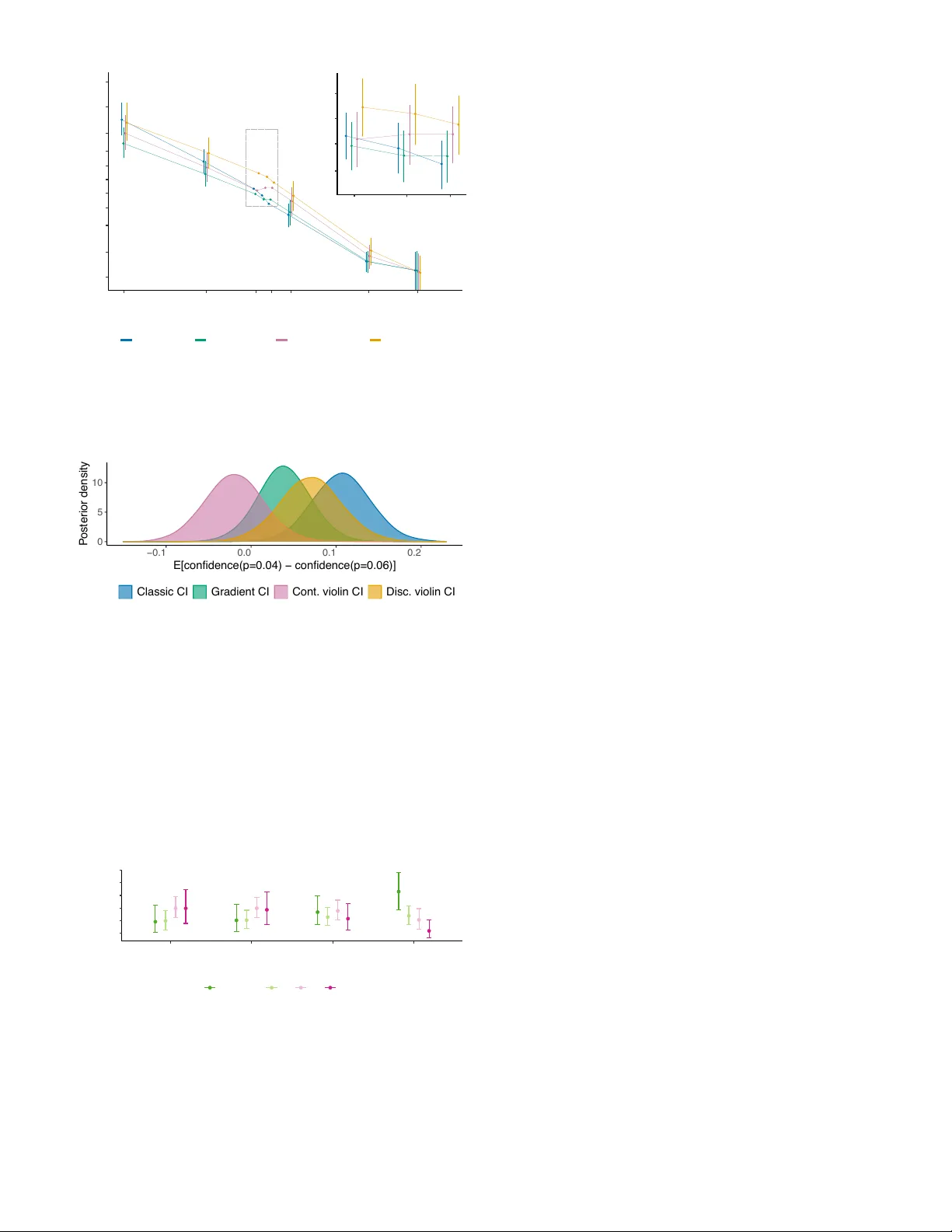
1 Can visualization alle viate dichotomous thinking? Eff ects of visual representations on the cliff eff ect Jouni Helske , Satu Helske , Matthew Cooper , Anders Ynnerman, Member , IEEE , and Lonni Besançon Abstract —Common repor ting styles for statistical results in scientiﬁc articles, such as p -values and conﬁdence intervals (CI), ha ve been repor ted to be prone to dichotomous interpretations, especially with respect to the null h ypothesis signiﬁcance testing framew ork. For example when the p -value is small enough or the CIs of the mean eff ects of a studied drug and a placebo are not overlapping, scientists tend to claim signiﬁcant differences while often disregarding the magnitudes and absolute diff erences in the effect sizes. This type of reasoning has been shown to be potentially harmful to science. T echniques relying on the visual estimation of the strength of e vidence hav e been recommended to reduce such dichotomous interpretations but their effectiv eness has also been challenged. We r an two experiments on researchers with expertise in statistical analysis to compare sev eral alternative representations of conﬁdence intervals and used Bay esian multile vel models to estimate the effects of the representation styles on diff erences in researchers’ subjective conﬁdence in the results. W e also asked the respondents’ opinions and preferences in representation styles . Our results suggest that adding visual information to classic CI representation can decrease the tendency towards dichotomous interpretations – measured as the ‘cliff effect’: the sudden drop in conﬁdence around p -value 0.05 – compared with classic CI visualization and textual representation of the CI with p -v alues. All data and analyses are pub licly av ailable at https://github .com/helske/statvis. Index T erms —Statistical inference, visualization; cliff eff ect; conﬁdence inter vals; h ypothesis testing; Bay esian inference . F 1 I ntroduction One of the most common research questions in many scientiﬁc ﬁelds is “Does X hav e an effect on Y?”, where, for example, X is a new drug, and Y a disease. Often the question is reduced to “Does the av erage ef fect of X differ from zero?”, or “Does X signiﬁcantly differ from Z?”. There are v arious statistical approaches av ailable for answering this question, and many ways to report the results from such analyses. In many ﬁelds, null hypothesis signiﬁcance testing (NHST) has long been the de-facto standard approach. NHST is based on the idea of postulating a “no-effect” null hypothesis (H0) which the experimenter aims to reject. An appropriate test statistic, based on assumptions about the data and model, is then calculated together with the corresponding p -value, the probability of observing a result at least as extreme as the one observed under the assumption that H0 is true. Small p -values indicate incompatibility of the data with the null model, assuming that the assumptions used in calculating the p -value hold. The ongoing ‘replication crisis’ [1], especially in social and life sciences, has produced many critical comments against arbitrary p -value thresholds and signiﬁcance testing in general (e.g., [2], [3], [4]). As a solution to av oid so-called dichotomous thinking – strong tendency to divide results into signiﬁcant or non-signiﬁcant – some are even arguing for a complete ban on NHST and p -values. Such a policy has also been adopted by some journals: e.g., in 2015, the Journal of Basic and Applied Social Psychology banned • J. Helske was with Department of Science and T echnology , Linköping University , Campus Norrköping, SE-602 74 Norrköping, Sweden, and now with Department of Mathematics and Statistics, University of Jyväskylä, FI-40014 Jyväskylä, F inland. E-mail: jouni.helske@iki.ﬁ • S. Helske is with Department of Social Resear ch, University of T urku, FI-20014 Turku, F inland. • M. Cooper , A. Ynnerman, and L. Besançon ar e with Department of Science and T echnology , Linköping University , Campus Norrköping, SE-60274 Norrköping, Sweden. Published in the IEEE T ransactions on V isualization and Computer Gr aphics. DOI: 10.1109/ TVCG.2021.3073466 both p -values and conﬁdence intervals (CIs) [5], and more recently the Journal of Political Analysis banned the use of p -v alues [6]. Despite the critique, signiﬁcance testing is likely to remain a part of a scientist’ s toolbox. Because many of the problems with NHST are due to misunderstandings among those who conduct statistical analyses as well as among those who interpret results, work has also been conducted in making it easier to av oid common pitfalls of NHST either by altering the way analyses are conducted [7], [8], [9] or how the results are presented [10], [11], [12], [13], [14]. Instead of arguing for better methodological solutions, such as Bayesian approaches, here we study whether different styles of visual representation of common statistical problems could help to alleviate dichotomous thinking which can be approximated by studying the so-called clif f effect [15]. The clif f ef fect is a term used for the large difference in how the results are interpreted despite only small numerical differences in the estimate and p -value [16] (e.g., the estimated effect of 0.1 with a corresponding p -value of 0.055 may be deemed not signiﬁcant while an effect of 0.11 with a p -value of 0.045 may be claimed to be signiﬁcant). In this paper we focus on the effect of visualization styles on conﬁdence proﬁles (the perceived conﬁdence–p-value relationship) and in particular on the magnitude of the cliff effect. T o study the potential cliff effect of various representation styles for statistical results, we conducted two experiments on researchers who are experienced in using and interpreting statistical analyses. W e showed participants results from artiﬁcial experiments using different representation styles and asked the respondents ho w conﬁdent they were in that the results showed a positiv e effect (experiment 1) or a difference between two groups (experiment 2). W e also asked the respondents to giv e comments on the different styles and to rank them according to their personal preference. W e analysed the answers from the experiments using Bayesian multilev el models. These results are easy to interpret and at the same time allow us to av oid the problems we aimed at studying (i.e. dichotomous thinking and the cliff effect). 2 Three earlier studies somewhat resemble our experimental setting. First, we use and compare similar visualizations of the uncertainty of the sample mean as Correll and Gleicher [12]. W e, howe ver , focus on a dif ferent research question and correspondingly a different target population. Correll and Gleicher were interested in the communication of mean and error to a general audience while our interest is in dichotomous thinking, by measuring the conﬁdence proﬁle and the cliff ef fect. W e are interested in the interpretations of quantitative scientiﬁc results, which requires a fundamental understanding of statistics. Hence we target researchers whose dichotomous interpretations can have adverse effects on conclusions and gained knowledge. Furthermore, addressing the question left open in [12], we also collected qualitative data on researchers’ preferences for different visualization styles. Lai [15], on the other hand, similarly to us focused on the magnitude of the cliff effect and the shape of the conﬁdence proﬁle. He manually categorized respondents’ conﬁdence proﬁles into four different categories, discarding a large proportion of answers which did not ﬁt into any category . Instead of comparing different visualization methods, he only used classic CI visualization. Third, Belia et al. [17] had a similar approach in that they also focused on experts’ (mis)conceptions of conﬁdence intervals (with researchers in medicine and psychology). Their focus was not on dichotomous thinking but on ﬁnding the positioning of tw o conﬁdence interv als so that the respecti ve groups would be deemed “statistically signiﬁcantly different”. Similarly to Lai, they only used classic CI visualization. Our contributions are as follows: 1) This is the ﬁrst study to examine the effects of visualization styles of CIs on conﬁdence proﬁles and dichotomous thinking (using the cliff ef fect as a proxy) among researchers. 2) W e are the ﬁrst to study researchers’ preferences on novel visualization styles in this context. 3) W e introduce the use of ﬂexible and easy-to-interpret Bayesian framework for the analysis of conﬁdence proﬁles and representation preferences. 4) As a contribution to open science, codes for the online experiment, data and all analyses are publicly av ailable and fully reproducible. Our results suggest that despite the increased debate around NHST and related concepts, the problem of dichotomous thinking persists in the scientiﬁc community , but that certain visualization styles can help to reduce the cliff effect and should be used and studied further . 2 B a ckground and R ela ted W ork In this paper, our main focus lies in whether and how different vi- sualizations can help in reducing the clif f effect among researchers making interpretations of inferential statistics. W e ﬁrst brieﬂy present the basic deﬁnition and interpretation of the conﬁdence in- terval (CI), which is a common choice for assessing the uncertainty of a point estimate (e.g., sample mean) and has sometimes been suggested to reduce dichotomous interpretations. W e then discuss the problem of dichotomous thinking in scientiﬁc reporting before presenting related literature and the visual representations used in our experiments. 2.1 Conﬁdence Interval f or Sample Mean Giv en a sample of values x 1 , . . . , x n from a normal distribution with unknown mean µ and variance σ 2 , the 95% conﬁdence interval for the mean is computed using a sample mean ¯ x , sample standard deviation s , sample size n and t -distrib ution: ¯ x ± t α / 2 ( n − 1 ) s √ n , (1) where t α / 2 ( n − 1 ) is the critical v alue from t -distribution with n − 1 degrees of freedom and signiﬁcance level α (typically 0 . 05 ). The interpretation of the (95%) CI is somewhat complicated: Giv en multiple 95% CIs computed from independent samples, on average 95% of these intervals will contain the true expected value µ . It is important to note that, given a single sample and the corresponding CI, we cannot infer whether the true population mean, µ , is contained within the CI or not [18] although it has a direct connection to NHST in that the 95% CI represents the range of values of µ for which the difference between µ and ¯ x is not statistically signiﬁcant at the 5% level. 2.2 The Prob lem of Dichotomous Thinking in Science Let us suppose that through an experiment we obtain a p -value of p = 0 . 048 . Most researchers would consider this strong enough evidence against H0. If, howe ver , we obtained p -value of 0.058 many researchers, despite the small difference, would follow the recommendations of colleagues and textbooks, consider this as not enough evidence against H0 [19]. This type of reasoning, often called dichotomous thinking or dichomotous infer ence has been shown to be potentially harmful to science [2], [20], [21], [22], [23]. It has been said to be one of the reasons for the replication crisis [20], [22], [24] or to lead to “absurd replication failures [with] compatible results” [2]. While dichotomous thinking has been heavily criticized by scholars (e.g., [10], [20], [21], [25], [26], it seems to be persistent in many ﬁelds including HCI [27] and empirical computer science [22]. In 2016, the confusion, misuse and critique around p -values led the American Statistical Association (ASA) to issue a statement on p -values and statistical signiﬁcance. ASA stated that proper inference must be based on full and transparent reporting and computing, and that a single number ( p -value) is not equal to scientiﬁc reasoning. Many other authors have criticized the whole NHST approach due to increased dichotomous thinking based on arbitrary thresholds [2], [19], [20], [26], [28], [29], common misinterpretations of p -values (e.g., the fallacy of accepting H0 [30], reading p -values as the probability that H0 is true), as well as the several questionable research practices that often come with the use of NHST including p -hacking (testing a number of hypotheses until a low p -value is found), HARKing (presenting a post-hoc hypothesis as an a priori hypothesis), selectiv e outcome reporting, and the ﬁle-drawer effect (limiting publication to only statistically signiﬁcant results) [22], [31], [32], [33], [34], [35], [36]. Additionally , sometimes p -values are reported without effect sizes, although a p -value itself does not help readers determine the practical importance of the presented results. It should be noted that it is likely that many of these issues relating to the data-led analysis (see the “garden of forking paths” [37] ) are typically not intentional, and can occur in a broader scope than just NHST . Due to all of the issues around p -values, some researchers hav e recommended either to replace or complement them with CIs [10], [26], [38], [39]. The argument is that CIs could reduce dichotomous interpretations as they represent both the effect size and the sampling variation around this value. CIs, howe ver , are also prone to misinterpretation, simply because their interpretation is not very intuitive [17], [40]. CIs have also been reported to lead to dichotomous thinking [15], [27], [41]. The term cliff effect was coined by Rosenthal and Gaito in their study [16] on 19 researchers in psychology . Their ﬁndings were later replicated by Nelson et al. [42] on a larger sample (85 3 psychologists). Poitevineau and Lecoutre [43] showed that only a small fraction of their participants adopted a dichotomous all- or-none strategy , while Lai [15] showed that milder tendencies to dichotomous thinking exist. Another study by Poitevineau and Lecoutre [44] suggested that ev en statisticians were not immune to misinterpretations and dichotomous thinking. Howe ver , due to the previous focus on restricted populations (mainly psychologists) and also because some of the details of the experiments ha ve not been fully presented (such as the exact question asked to the participants), it is difﬁcult to assess whether these ﬁndings would hold in a more general population of researchers. Previous studies on interpretation of p -values and CIs have suggested that there are two to four conﬁdence interpretation proﬁles [13], [15], [43]. While some indi vidual v ariation and hybrid interpretation styles are likely to exist, due to historical reasons it is likely that the main proﬁles are the all-or-none category (related to Neyman-Pearson signiﬁcance testing) and the gradually decreasing conﬁdence category (related to Fisher’ s signiﬁcance testing approach). See, for example, [45] for descriptions of the original approaches to signiﬁcance testing by Fisher, and Neyman and Pearson as well as their connection to current NHST practice. Bayesian paradigm and replacing CIs with credible intervals hav e been suggested as a solution to the problems with CIs and p -values [7], [8], [46], [47]. Compared to the CI, the credible interval has a more intuitiv e interpretation: giv en the model and the prior distribution of the parameter (e.g., mean), the 95% credible interval contains the unknown parameter with 95% probability . Or perhaps e ven better , one can present the whole posterior distrib ution of the parameter of interest. Despite the beneﬁts of the Bayesian approach, p -values and CIs are likely to remain in use in many scientiﬁc ﬁelds, despite their ﬂaws. Hence it is of general interest to study whether the problems relating to dichotomous thinking can be alleviated by changing their typical representation styles. 2.3 Visualization of Uncertainty and Statistical Results Sev eral visualization techniques have been designed to show the uncertainty of the estimation, with several advantages over the communication of a sole point estimate [48], [49]. Showing the theoretical or empirical probability distribution of the variable of interest is a commonly used technique. For example, probability density plots are often used for describing the known distributions such as Gaussian distribution or estimated density functions based on samples of interest (e.g., observ ed data or samples from posterior distributions in a Bayesian setting). V iolin plots [50] (also called e yeball plots in [51]) are rotated and mirrored kernel density plots, so that the uncertainty is encoded as the width of the ‘violin’ shape. Raindr op plots [52] are similar to violin plots but are based on log- density . The gradient plot uses opacity instead of shape to con vey the uncertainty (e.g., [12]), while quantile dot plots [53], [54] are discrete analogs of the probability density plot. V arious alternativ e representation styles speciﬁcally for CIs are commonly used (see, for example, [55]). In order to remedy the misunderstanding and misinterpretation of CIs, Kalinowski et al. [13] designed the cat’s e ye conﬁdence interval which uses normal distributions to depict the relative likelihood of v alues within the CI (based on the Fisherian interpretation of the CI). A violin plot with additional credible interval ranges are also used to depict arbitrary shaped (univ ariate) posterior distributions based on posterior samples, for example in the tidybayes R package (coined as the eye plot ) [56]. Kale et al. [57], [58] studied animated hypothetical outcome plots for interactive dissemination of statistical results. Going even further , Dragicevic et al. [14] propose the use of interactiv e explorable statistical analyses in research documents to increase their transparency . For a systematic revie w of uncertainty visualization practices, see Hullman et al. [59]. Some past studies have focused on comparing different visual representations of statistical results. T ak et al. [60] examined seven different visual representations of uncertainty on 140 non-experts. Correll and Gleicher [12] studied four different visualization styles for mean and error in several settings. Kalinowski et al. [13] compared students’ intuitions when interpreting classic CI plots and cat’ s eye plots. Finally , the recent study by Hofman et al. [58] focused on the impact of presenting inferential uncertainty in comparison to presenting outcome uncertainty , and inv estigated the effect of different visual representations of effect sizes. With the exception of [13], these studies hav e focused on testing lay-people, a population which can be expected to differ from researchers who hav e been trained to interpret p -values and CIs in their work. 3 R esearch Q uestions T aking inspiration from some of the approaches listed in Section 2, our work aims to ev aluate the presence and magnitude of the cliff effect in textual and visual representation styles among researchers trained in statistical analysis. Our main goals were to inv estigate • whether the cliff effect can be reduced by using different visual representations instead of textual information and • how researchers’ opinions on, and preferences between, different representation styles differ . More speciﬁcally , we were interested in whether the previously documented cliff effect in scientiﬁc reporting is reduced when the textual representation with explicit p -value is replaced with a traditional visualization of CI, and whether more complex visualization styles for the CI reduce the cliff effect. Regarding the former question, in line with previous research [15], [41], we expected to ﬁnd that CIs would not reduce the cliff effect, whereas regarding the latter question our hypothesis was that more complex visualization styles could reduce the cliff effect. As our interest was in scientiﬁc reporting, we limited our sample to researchers with an understanding and use of statistics unlikely to be present with lay-people, and focused on static visualizations applicable in traditional scientiﬁc publications. While researchers are more familiar with conﬁdence intervals and other statistical concepts, experts’ interpretations can still exhibit various implicit biases and errors due to ﬁeld’ s conv entions and obtained education (see, e.g, [61]). Howe ver , instead of studying the differences in various subgroups of scientiﬁc community , our interest is more about an "average researcher". 4 O ne - sample E xperiment In the ﬁrst experiment we are interested in potential differences in the interpretation of results of an artiﬁcial experiment when partici- pants are presented with textual information of the experiment in a form of a p -value and a CI, a classic CI plot, a gradient CI plot, or a violin CI plot (see Fig. 1 and the descriptions in subsection 4.1). The setting is simple yet common: we ha ve a sample of independent observations from some underlying population, and we wish to infer whether the unknown population mean differs from zero. 4 Mean weight increase 0.817kg, 95% CI: [−0.036kg, 1.669kg], p = 0.06 (2−sided t−test) Fig. 1. Representation styles used in the experiments: T extual v ersion with p -value , classic 95% conﬁdence inter val (CI), gr adient CI plot, violin CI plot, and discrete violin CI plot. 4.1 Conditions 4.1.1 T e xtual Information with p -value Our ﬁrst representation is text consisting of the exact p -value of a two-sided t -test, sample mean estimate and lo wer and upper limits of the 95% CI (see the leftmost box of Fig. 1 for the participant’ s view). This style is concise, contains information about the effect size and the corresponding variation (width of the CI), while the p -value provides evidence in the hypothesis testing style. While this format provides information on the effect size and uncertainty together with the p -valueit can be argued that, due to the strong tradition in NHST , the inclusion of a p -value can cause dichotomous thinking even when accompanying CI information is provided. While the sample size is not stated in this format, that information was provided separately in our experiment for each condition as a part of the explanatory text. 4.1.2 Classic Conﬁdence Inter v al Visualization Conﬁdence interv als and sample means are commonly visualized as line segments with end points augmented with horizontal lines (see Fig. 1). Compared with textual information, visual representation could be better at conv eying the uncertainty . While the width of the horizontal lines of the CI does not have semantic meaning, it is sometimes argued (although we have found no studies to suggest this) that their width emphasises the limits of the CI and increases dichotomous inference, and intervals without the horizontal lines should be preferred. W e chose the more traditional design (see the second box from left in Fig. 1) as it is still commonly used and is a default in many statistical analysis packages such as SPSS. 4.1.3 Gradient Color Plot f or CI (Gradient CI Plot) In order to reduce the dichotomous nature of the classic CI visualization, we test the effect of using multiple overlaid con- ﬁdence intervals with varying coverage levels and opacity . This is fairly common when presenting prediction intervals for future observations [62], but less so in the case of CIs. While using only a few overlaid CIs (e.g., 80%, 90% and 95%) is a more common practice, we decided to replicate the gradient plot format used in previous approaches [12] which provides more emphasis on the 95% interval and thus is more comparable with the classic CI approach. Our gradient CI plot contains a colored area of 95% CI complemented with gradually colored areas corresponding to 95.1% to 99.9% CIs (with 0.1 percentage point increments), ov erlaid with a horizontal line corresponding to the sample mean (see the middle box in Fig. 1). The coloring was from hex color #2ca25f to #e5f5f9 taken from ColorBre wer’ s 3-class BuGn palette [63]. This format provides additional information, but gradual color changes can be difﬁcult to interpret accurately , and from a technical point of view this format is also harder to create than classic CIs. 4.1.4 CI as t -violin Plot (Violin CI Plot) While the gradient CI plot giv es information about the uncertainty beyond the 95% CI, we claim that the use of the rectangular regions with constant widths can be misleading. Therefore, as our fourth representation format (inspired by [12], [13]) we combine the gradient CI plot and the density of the t -distribution used in constructing the CIs (see the second box from right in Fig. 1). More speciﬁcally , in the violin CI plot the shape corresponds to the case of computing a sequence of conﬁdence intervals with very ﬁne increments, with the width of each CI computed using the underlying t -distrib ution. The width of the violin at point y is p ( √ n ( y − ¯ x ) s ) √ n s , (2) where p is the probability density function of the t -distribution with n − 1 degrees of freedom, ¯ x is the sample mean, and s is the standard deviation. In the second experiment we also consider a more discretized version of the violin CI plot with gradually colored areas corre- sponding to the 80%, 85%, 90%, 95% and 99.9% CIs (see the rightmost box in Fig. 1). V iolin CI plots are more challenging to create, and the probability density function style can lead to erroneous probability interpretations for which CIs cannot provide answers. On the other hand, the additional visual clues due to the shape can help o vercome the difﬁculty of interpreting gradient colors. 4.2 P ar ticipants and Apparatus The experiment was run as an online surve y . Its preregistration is av ailable on https://osf.io/v75ea/. As the preregistration states, the number of participants was not decided in advance but, instead, we aimed for the maximum number of participants in a gi ven time frame. The end date of the experiment was ﬁxed to 11 March 2019 so the surve y was open for 21 days before we started to analyse the data. As stated in section 3, our goal, contrary to most of the previous work, was to understand how researchers interpret statistical results and therefore we aimed at recruiting academics familiar with statistical analysis. T o recruit participants across various scientiﬁc disciplines, we initially contacted potential participants via email in sev eral ﬁelds (namely Human Computer Interaction, V isualization, Statistics, Psychology , and Analytical Sociology , using personal networks), and the survey was also shared openly using the authors’ academic proﬁles on T witter and suitable interest groups on Reddit, LinkedIn, and Facebook. 5                 0 1 2 0.001 0.01 0.04 0.05 0.06 0.1 0.5 0.8 p− value Weight increase (kg) Sample size 50 200 Fig. 2. Conﬁguration used in the one-sample experiment. See text f or details. The eligibility criteria were 1) Y ou understand English; 2) Y ou are at least 18 years old; 3) Y ou have at least a basic understanding of hypothesis testing and conﬁdence intervals; 4) Y ou use statistical tools in your research projects; 5) Y ou are not using a handheld device such as tablet or phone to ﬁll out the survey . T o ev aluate the validity of our sample, we asked for background information including participants’ age, scientiﬁc ﬁeld, highest academic de gree, length of research experience, and data analysis tools commonly used. The codes for the experiment are available in supplementary materials on https://github.com/helske/statvis. There are multiple potential factors which could (although not necessarily should) have an effect on interpreting results of this simple experiment: p -value, total length of the conﬁdence interval, effect size, sample size, and representation style. Since our focus was on the representation styles, and because we wanted to keep the survey short in order to increase the number of responses, we used a ﬁxed set of p -values (0.001, 0.01, 0.04, 0.05, 0.06, 0.1, 0.5, 0.8), and a ﬁxed standard deviation of 3. By deﬁning also the sample size, the sample mean was then fully determined by these values. W e used two sets of questions, one with a sample size of n = 50 and another with n = 200 . Each participant saw the results corresponding to only one of these sets. Fig. 2 shows the conﬁgurations as 95% CIs with dots representing the means. The participants did not see the underlying p -values except in the textual representation style. During the experiment we displayed each trial to each par- ticipant (one at a time), and asked the following question: “ A random sample of 200 adults from Sweden were prescribed a new medication for one week. Based on the information on the screen, how conﬁdent are you that the medication has a positive effect on body weight (increase in body weight)?”. They answered on a continuous scale (100 points between 0 and 1, the numerical value was not sho wn) using a slider with labelled ends (“Zero conﬁdence”, “Full conﬁdence”), which was explained to the participants as “Leftmost position of the slider corresponds to the case “I hav e zero conﬁdence in claiming a positive effect, ” whereas the rightmost position of the slider corresponds to the case “I am fully conﬁdent that there is a positiv e effect. ” The slider’ s ‘thumb’ was hidden at ﬁrst, in order to av oid any possible bias due to its initial position. It only became visible when the participant clicked on the slider . Finally , until the slider position was set participants could not proceed to the next question. Our small pilot study suggested that it was hard to understand the violin CI plot due to its non-standard meaning (participants were prone to misread the ﬁgure as a typical violin plot of empirical density of the data). Therefore, in order to e xplain the interpretation of the violin plot in this context, we had to also explain the basics of CI computations. T o keep the complexity of all representations at the same lev el, we added explanatory texts to all conditions. W e detail the impact of this decision in our discussions in section 6 In order to balance learning effects, the order of the four conditions (representation styles) was counterbalanced using Latin squares, and within each condition the ordering of trials was randomly permuted for each participant. At the end of the surve y , participants had to give feedback on the representation formats and rank them from 1 (best) to 4 (worst). W e gav e participants the possibility to giv e equal rankings. They could also leave additional comments about the survey in general. W e gathered answers from 114 participants, from which one participant was excluded because of nonsensical answers to the background questions. One of the background variables was an open-ended question about ﬁeld of expertise. The answers included a range of disciplines that we categorized into four groups: “Statistics and machine learning’ (21 participants), “VIS/HCI” (34), “Social sciences and humanities” (32), and "Physical and life sciences" (26) (see supplementary material for more information). 4.3 Statistical methods All statistical analyses were done in the R en vironment [64] using the brms package [65]. The visualizations of the results were created with the ggplot2 package [66]. The collected data, scripts used for data analysis, additional analysis, and ﬁgures are av ailable in supplementary material. W e also created an accompanying R package ggstudent 1 for drawing modiﬁed violin and gradient CI plots used in the study . T o analyse the results we built a Bayesian multile vel model with participants’ conﬁdence as the response variable (values ranging from 0 to 1), and the underlying p -value and representation style as the main explanatory variables of interest. While we often perceiv e the probabilities and strength of evidence as having a linear relationship after logit-transformations of both variables [67], in the case of signiﬁcance testing with potential for dichotomous thinking this relationship is likely not true due to the potential cliff ef fect as well as the excess occurrence of low and high p -values indicating complete lack of evidence (0) or full conﬁdence (1). V alues 0 and 1 (15% of all answers) are also problematic in the logit-transformation due their mapping to ± ∞ . Therefore, a simple linear model with logit-transformations of p -values and the conﬁdence scores would not be suitable in this case. A typical choice for modelling proportions with disproportion- ately large numbers of zeros and ones is the zero-one-inﬂated beta regression. Howe ver , as we wanted to incorporate the prior knowledge of the potential linear relationship of conﬁdence and probabilities in the logit-logit-scale, instead of the zero-one-inﬂated beta distribution we created a piecewise logit-normal model 2 with the probability density function (pdf) deﬁned as p ( x ) =      α ( 1 − γ ) , if x = 0 , α γ , if x = 1 , ( 1 − α ) φ ( logit ( x ) , µ , σ ) , otherwise . (3) Here α = P ( x ∈ { 0 , 1 } ) is the probability of answering one of the extreme values (not at all conﬁdent or fully conﬁdent), whereas 1. https://cran.r- project.or g/package=ggstudent 2. The distribution was changed from the preregistration as suggested by a revie wer and [67]. 6 T ABLE 1 The sample mean, standard deviation, standard error of the mean, and the 2.5th and 97.5th percentiles of the difference in conﬁdence when p = 0 . 04 and p = 0 . 06 in the ﬁrst experiment. Mean SD SE 2.5% 97.5% T extual 0.19 0.27 0.03 -0.19 0.72 Classic CI 0.23 0.25 0.02 -0.05 0.84 Gradient CI 0.10 0.24 0.02 -0.37 0.74 V iolin CI 0.13 0.20 0.02 -0.16 0.62 γ = P ( x = 1 | x ∈ { 0 , 1 } ) , is the conditional probability of full conﬁdence given that the answer is one of the extremes 3 . Thus these two parameters model the extreme probability of answers, and when the answer is between the extremes, we model it with the logit-normal distribution ( φ ( x ) is the pdf of the normal distribution parameterized with mean µ and standard deviation σ ). Explanatory variables can be added to the model to predict α , γ , µ , and σ , using the log-link for σ , the logit-link for α and γ , and the identity-link for µ . In comparison to the frequentist approach, such as standard generalized linear (mixed) models or analysing only simple descriptive statistics, our Bayesian model allows us to take into account the uncertainty of the parameter estimation and more ﬂexible model structures. W e can also make various simple probabilistic statements based on the posterior distributions of this model such as the probability that the cliff effect is higher with p -values than with classic CI. For further information about Bayesian modelling in general see, for example, [68]. 4.4 Results 4.4.1 Conﬁdence Proﬁles and Cliff Eff ects As the ﬁrst step, we checked some descriptiv e statistics of the potential cliff effect, deﬁned as δ = E [ conﬁdence ( p = 0 . 04 ) − conﬁdence ( p = 0 . 06 )] , i.e., the average difference in conﬁdence between cases p = 0 . 04 and p = 0 . 06 . T able 1 shows how gradient and violin CI plots hav e a somewhat smaller drop in conﬁdence when moving from p = 0 . 04 to p = 0 . 06 compared to the textual representation and the classic CI visualization. T o analyse the data and the potential clif f effect in more detail, we used the Bayesian multilev el model described in subsection 4.3. Due to the setup of the experiment, participants’ answers were inﬂuenced by the information on the screen, which in turn depended on the underlying p -value, visualization style, and sample size. Sample size itself should not hav e an effect on the answers, which was indeed conﬁrmed by preliminary analysis (see supplementary material), so we dropped that variable from further analysis. Due to the potential cliff effect we wanted to allow different slopes of the conﬁdence curve for the cases when p < 0 . 05 and p > 0 . 05 . W ith regards to the case of p = 0 . 05 we allowed an extra drop in conﬁdence via an indicator variable I ( p = 0 . 05 ) , as it was not clear whether this boundary case should be on the “signiﬁcant” or “not signiﬁcant” side (i.e., whether the cliff effect was due to the drop just before or after 0.05). Regarding the probability of an extreme answer , the relationship with respect to the p -value was assumed to be non-linear so we treated the p -values as a categorical variable. 3. While generating data from this distribution is straightforward, the expected value of this distribution is analytically intractable. Howe ver , this can be easily computed via Monte Carlo simulation. For the conditional probability of full conﬁdence γ we used the p -value as a categorical variable with a monotonic effect (using the simplex parameterization suggested in [69]), but grouped p > 0 . 05 values together . As it was reasonable to assume that participants used different scales of conﬁdence in their answers (e.g., some participants were always very conﬁdent), we included individual-le vel random intercepts for µ , α and σ . W e also allowed the effects of visual- ization and the underlying p -value to vary between participants by including corresponding random coefﬁcients in the model. W e ran various posterior predictiv e checks [70] to assess that the model ﬁts the data reasonably well (see the supplementary material). The ﬁnal model structure, written using the extended W ilkinson-Rogers syntax [71], [72] was chosen as follows: µ ∼ viz · I ( p < 0 . 05 ) · logit ( p ) + viz · I ( p = 0 . 05 ) + ( viz + I ( p < 0 . 05 ) · logit ( p ) + I ( p = 0 . 05 ) | id ) , α ∼ p · viz + ( 1 | id ) , γ ∼ mo ( p ) , σ ∼ viz + ( 1 | id ) , (4) where p is a categorical variable deﬁning the true p -value, logit( p ) is a continuous variable of the logit-transformed p -value, mo ( p ) denotes a monotonic effect of the p -value, the dot corresponds to interaction (i.e., I ( p = 0 . 05 ) · viz implies both the main and two-way interaction terms) and ( z | id ) denotes participant-level random effect for variable z . Giv en this model, in a presence of a cliff effect we should observe a discontinuity in an otherwise linear relationship between the true p -valueand reported conﬁdence (when examined in the logit-logit scale). W e used the relativ ely uninformativ e priors: N ( 0 , 5 ) regression coefﬁcients, N ( 0 , 3 ) for the intercept terms, and half-N ( 0 , 2 ) for all standard deviation parameters, LKJ(1) prior [73] for the correlation matrices of random effects, and symmetric Dirichlet(1) prior for the coefﬁcients of the monotonic effect. Consistent with the Bayesian paradigm, we chose this model ov er simpler submodels (where some of the interactions or random effects are omitted) [74]. This model integrates over the uncertainty regarding the model parameters, with coefﬁcient zero corresponding to a simpler model where the term is omitted from the model. Ho wev er , as a sensitivity check, we also estimated sev eral submodels of this model. These gave very similar results, so the reported results were insensitive to speciﬁc model choice. Fig. 3 shows the posterior mean curves of conﬁdence (vertical lines corresponding to the 95% credible intervals 4 ) with respect to the underlying true p -values used to generate the data. These are based on the population lev el effects: the expected conﬁdence of an average participant (an individual whose random effects are 0). W e observe at least some kind of a cliff effect – a sudden drop in conﬁdence – with all representation styles. Within the “statistically signiﬁcant region” (i.e., when p < 0 . 05 ) the slope of the conﬁdence level in relation to the underlying p -value is the least steep for the classic CI visualization, but there is a large drop in conﬁdence when moving to p > 0 . 05 , even larger than with the textual information. The textual representation with p -value, on the other hand, behaves similarly to the violin CI plot until p = 0 . 05 , after which the conﬁdence in the p -value representation drops below all other techniques. The gradient CI plot and the 4. For readers new to the credible interval, we refer to section 2.2. 7 0.4 0.5 0.6 0.7 0.8 0.04 0.05 0.06 0.05 0.1 0.2 0.3 0.4 0.5 0.6 0.7 0.8 0.9 0.95 0.001 0.01 0.04 0.06 0.1 0.5 0.8 p− value Confidence T extual Classic CI Gradient CI Violin CI Fig. 3. Posterior means of conﬁdence and corresponding 95% credible intervals for diff erent visualization styles in the ﬁrst e xperiment, on the logit- logit-scale. Here, a discontin uity in an otherwise linear relationship indicates a cliff eff ect. The zoom-in plot shows the uncer tainty of the estimates when 0 . 04 ≤ p ≤ 0 . 06 . violin CI plot both have a smaller – although visible – drop in conﬁdence and also otherwise show a similar pattern, except that the conﬁdence level of the gradient CI plot is constantly below that of the violin CI plot. The range of conﬁdence is very similar across all representation styles, which suggests that the smaller cliff effect of gradient CI and violin CI plot is not to due to ov erall smaller conﬁdence (not an unreasonable assumption giv en their more fuzzy nature compared to classic CI). There were no clear differences in the probabilities of an extreme answer (“zero conﬁdence” or “full conﬁdence”) between the visualization styles (see the supplementary material). Fig. 4 shows the posterior distributions of the drop in conﬁ- dence, δ , for different visualizations. These show that the drop is the largest with classic CI and the smallest (and nearly identical) with gradient and violin CI visualizations. T extual representations with p -values position between these (somewhat closer to the classic CI). The magnitude of the drop in the classic CI (mean of 0.29) is close to a third of the range of the conﬁdence scale and twice as large as the drop in the gradient and violin CIs (means of 0.15). While there is some ov erlap between these distributions, when comparing the pairwise posterior probabilities that the δ of one visualization style is greater than that of an alternativ e style for an av erage participant (T able 2), we see clear differences between the styles: Classic CI leads to larger drop than textual p -values, and both of these lead to larger drops than Gradient CI and V iolin CI (all these comparisons have probabilities close to 1). Note that, unlike the interpretation of p -values, the numbers in T able 2 are actual probabilities that the average drop in conﬁdence around p = 0 . 05 is larger with one style than the other . As a secondary analysis, we also estimated a model with categorized expertise value as a predictor (with interactions with visualization and p -value). When av eraging (i.e. marginalizing) ov er the expertise, the results were similar to the main model. The expertise-speciﬁc examinations, howe ver , revealed some dif- ferences between the groups. Most notably we observed the largest cliff effects in the Stats/ML group (for all representation styles), while in the Phys/Life group there were only small differences in the conﬁdence proﬁles by representation style. When comparing 0 5 10 15 0.1 0.2 0.3 E[confidence(p=0.04) − confidence(p=0.06)] P oster ior density T e xtual Classic C I Gr adient CI Violin CI Fig. 4. P osterior distributions of δ , the drop in conﬁdence around p = 0 . 05 , for different representation styles in the ﬁrst experiment. Note that the distributions of the gradient CI and the violin CI on the left-hand side are almost completely ov erlapping. T ABLE 2 P osterior probability that δ , the drop in conﬁdence around p = 0 . 05 , is larger for representation style on the ro w than the representation style on the column. T extual Classic CI Gradient CI V iolin CI T extual - 0.01 1.00 1.00 Classic CI 0.99 - 1.00 1.00 Gradient CI 0.00 0.00 - 0.49 V iolin CI 0.00 0.00 0.51 - the magnitudes of δ , the ordering of the representation styles was the same across all expertise groups (as seen in the main results). Due to space restrictions see the supplementary material for more detailed results. 4.4.2 Subjective Rankings T o analyse the subjectiv e rankings of the representations, we estimated a Bayesian ordinal regression model where we used visualization style to predict the observed rankings (with participant- lev el random intercept). Fig. 5 shows the results from this model as a probability that the visualization style obtains a certain rank. W e see that p -value typically obtains the worst rank (4), while violin CI and classic CI are the most preferred options with approximately equal probabilities for ranks 1 and 2. Gradient CI seems to divide opinions, with close to equal probabilities for each rank. 4.4.3 Qualitative F eedback At the end of the experiment, participants were in vited to comment on the limitations and beneﬁts of each technique. The fully categorized and raw data is av ailable in supplementary materials, but we summarize the main points here. The following summaries were created by one of the authors before seeing any of the other results. Concerning p -values, participants reported them to be easy to read and accurate ( × 40 participants). Howe ver , participants also stated that they could hinder the readability of a paper if many of them had to be reported ( × 11), that they could be difﬁcult to interpret ( × 33), that some expertise was needed to understand them ( × 10), and that text-only might make readers focus on p - values exclusi vely ( × 7). Furthermore, some participants explained that a visualization would have made the analysis much easier, in particular for the conﬁdence interval ( × 22). The condition with classic conﬁdence intervals was said to be a standard ( × 19) that allows quick analysis with clear ﬁgures ( × 42) and that scales very well to multiple comparison ( × 11). Howe ver , participants also reported that this visual representation was missing information — likelihood of the tails for instance— and that it should be augmented with more statistical information ( × 33). Additionally , they were 8 0.1 0.2 0.3 0.4 0.5 T e xtual Classic CI Gradient CI Violin CI Representation Ranking probability 1 (best) 2 3 4 (worst) Fig. 5. Subjective r anking probabilities and the corresponding 95% credible intervals for visualization styles of the ﬁrst one-sample e xperiment. A higher value f or rank 1 indicates pref erence for the method while a higher v alue for rank 4 indicates distaste. said to possibly foster dichotomization ( × 10). V iolin CI plots were judged to be visually pleasing ( × 8), to provide all the statistical information that classic conﬁdence intervals fail to provide ( × 31) and to help av oiding the dichotomization pitfall ( × 5). Nonetheless, some participants stated that they were representing too much information ( × 4), that they might require training as they are not often used ( × 17), and that the gradient at the tails was hard to see ( × 13). In addition to this, some participants explained that such plots could be misunderstood due to their similarity with the violin plot ( × 6). Finally , the gradient CI plots were reported to be visually pleasing ( × 5), to provide more information than a classic conﬁdence interval ( × 20), to help av oiding dichotomization ( × 6). In addition to this, participants stated (either as a positive or negativ e point) that the cut off after 95% was dif ﬁcult to assess visually ( × 9) which could also help reduce dichotomized interpretations. Participants also noted that the gradient was hard to distinguish ( × 9), that making inferences based on gradient plots could be more difﬁcult ( × 11) and that the width was unnecessary visual information because it does not encode anything ( × 13). 5 T wo - sample E xperiment After conducting the ﬁrst experiment, we deployed a second surve y with a similar framing, but this time instead of comparing the base value of zero, the task was to compare means of independent “treatment” and “control” groups, as in [17]. While it is often recommended that instead of comparing intervals of two (potentially dependent) samples it is better to compare intervals of the difference [75], nev ertheless these types of multiple interval visualizations are commonly seen in scientiﬁc publications. Similar to our ﬁrst controlled e xperiment, this study w as also preregistered 5 , with supplementary material av ailable at Github . 6 Fig. 6 shows the conﬁguration used in this second experiment. 5.1 Conditions, P ar ticipants and Apparatus The conditions and overall design of the study were the same as the one-sample experiment except that the textual p -value representation was replaced with a more discrete version of the violin plot (see rightmost ﬁgure in Fig. 1). The question w as framed as “ A random sample of 50 adults from Sweden were prescribed a new medication for one week. Another random sample of 50 adults from Sweden were assigned to a control group and giv en a placebo. Based on the information on the screen how conﬁdent are you that the medication decreases the body weight? Note the y-axis, higher values correspond to larger weight loss. ”. The slider 5. https://osf.io/brjzx/?view_only=e481a9ad345e4e689799d65d988c1c5f 6. https://github.com/helske/statvis                 1.0 1.5 2.0 0.001 0.01 0.04 0.05 0.06 0.1 0.5 0.8 p− value Weight decrease (kg) Group Control T reatment Fig. 6. Conﬁguration used in the second e xperiment. T ABLE 3 The sample mean, standard deviation, standard error of the mean, and the 2.5th and 97.5th percentiles of the difference in conﬁdence when p = 0 . 04 and p = 0 . 06 in the second experiment. Mean SD SE 2.5% 97.5% Classic CI 0.07 0.12 0.02 -0.22 0.28 Gradient CI 0.01 0.12 0.02 -0.21 0.25 Continuous violin CI 0.01 0.09 0.01 -0.15 0.17 Discrete violin 0.06 0.18 0.03 -0.17 0.50 endpoints were labelled “I hav e zero conﬁdence in claiming an effect”, and “I am fully conﬁdent that there is an effect. ”. For this second experiment we used the same channels for sharing the link as in the ﬁrst study and obtained 39 answers, of which two were discarded as they had not answered the background questions. Nine participants had expertise in “Statistics and machine learning”, eight in “VIS/HCI”, 14 in “Social sciences and humanities” and six in “Physical and life sciences”. 5.2 Results 5.2.1 Conﬁdence Proﬁles and Cliff Eff ect T able 3 shows the dif ferences between subjective conﬁdence when the underlying p -value was 0.06 versus 0.04. The drop in conﬁdence is again the largest with the classic CI with discrete violin CI having a similar drop. The relativ ely large standard error in the case of the discrete violin CI is explained by a small number of respondents that demonstrated a very large drop in conﬁdence with the discrete violin CI. Overall the cliff effect seems to be much smaller than in the one-sample case (where the average drop was between 0.15–0.30, depending on the technique). For analysing the results, we used the same multilevel model as for the ﬁrst experiment. Fig. 7 and Fig. 8 show the posterior mean curves of conﬁdence and the posterior distributions of δ (the drop in conﬁdence around 0.05). Compared with the ﬁrst experiment, the ov erall conﬁdence le vels are smaller , for example with p = 0 . 04 the av erage conﬁdence is about 0.5 compared to 0.7 in the ﬁrst experiment. There is a peculiar rise in the av erage conﬁdence lev el for the continuous violin CI when the underlying p -value is 0.05 and 0.06 (although the credible intervals are wide) but, overall, the differences between visualization styles are relatively small. Also, in contrast with the one-sample experiment, here we do not see clear signs of cliff effect or dichotomous thinking as the posterior mean curves are approximately linear (except, perhaps, for the classic CI where the posterior mean of δ is 0.1). As in the ﬁrst experiment we saw no clear differences in the probability of an extreme answer between visualization styles. 9 0.3 0.4 0.5 0.6 0.04 0.05 0.06 0.05 0.1 0.2 0.3 0.4 0.5 0.6 0.7 0.8 0.9 0.95 0.001 0.01 0.04 0.06 0.1 0.5 0.8 p− value Confidence Classic CI Gradient CI Cont. violin CI Disc. violin CI Fig. 7. Posterior means of conﬁdence and corresponding 95% credible intervals for different visualization styles in the second experiment, on logit-logit-scale, with a zoom-in plot of the cases with 0 . 04 ≤ p ≤ 0 . 06 . A discontinuity in otherwise linear relationship between the true p -value and repor ted conﬁdence indicates a cliff effect. 0 5 10 −0.1 0.0 0.1 0.2 E[confidence(p=0.04) − confidence(p=0.06)] P oster ior density Classic CI Gr adient CI Cont. violin CI Disc. violin CI Fig. 8. P osterior distributions of δ , the drop in conﬁdence around p = 0 . 05 , for diff erent visualization styles in the second experiment. 5.2.2 Subjective Rankings As in the ﬁrst experiment, we analysed the subjective rankings of the representation styles by Bayesian ordinal regression model where we explained the rank with visualization style and individual variance. Fig. 9 presents the ranking probabilities which indicate preferences towards the discrete violin CI plot (estimated to be the most preferred style by 42% of the respondents). No clear differences emerge between other styles, and especially the classic CI and the gradient CI yield very similar results. 0.1 0.2 0.3 0.4 0.5 0.6 Classic CI Gradient CI Cont. violin CI Disc. violin CI Representation Ranking probability 1 (best) 2 3 4 (worst) Fig. 9. Subjective r anking probabilities and the corresponding 95% credible intervals for visualization styles of the second experiment. A higher value f or rank 1 indicates preference for the method while a higher value for rank 4 indicates distaste. 5.2.3 Qualitative F eedback For this second controlled experiment, participants were also asked to comment on the limitations and beneﬁts of each visualization. The fully categorized and raw data is, again, available in the supplementary material and we present the most frequent comments here. Classic CIs were reported as easy to read and analyse ( × 12), space-efﬁcient and a scalable visual representation ( × 5), and as a standard visualization technique ( × 5). Y et, some participants stated that they might call for dichotomous interpretations ( × 5) and that they lack some information ( × 12). Continuous violin CI plots were said to provide more information than a classic CI ( × 2), but participants complained about the lack of explicit markers for the CI ( × 6) and that the gradient was hard to see ( × 3). Concerning discrete violin CI plots, participants noted that they are visually pleasing ( × 2), that they provide more information than classic CIs ( × 10) and that seeing the discrete steps was very helpful— in comparison with the continuous violin plot ( × 7). Still some participants highlighted that the gradient was hard to see ( × 3) and that these plots could provide too much information in a single ﬁgure ( × 2). Finally , gradient plots were deemed easy to interpret ( × 8) but participants noted that the width was unnecessary ( × 3), that some information was missing compared to gradient plots ( × 4), and that the gradient was difﬁcult to see ( × 8). 6 D iscussion In line with previous ﬁndings [15], [41], our results conﬁrm that the classic CI visualization does not ﬁx the cliff effect problem documented to be present in numerical and textual information. In fact, it appears that it may even incr ease the cliff effect. At the same time, many participants preferred the graphical presentation of CIs over text, stating reasons such as the CI plot being clear and quick to grasp as well as scaling very well to multiple comparisons. W e found that more complex visualization styles reduced the cliff effect in the ﬁrst one-sample e xperiment, and the violin CI plot, in particular, was also well receiv ed by the participants. W e found no clear differences between the interpretation of violin CI and gradient CI plots, which is in line with [12]. While we e xpected that these more novel visualization styles (violin and gradient CI plots) would introduce additional problems with interpretation due to unfamiliarity , their beneﬁts seem to outweigh these negati ve ef fects. Some of the problems with violin CI plots could be explained by confusion with typical uses of a violin plot (as suggested by our feedback), namely as a method of visualizing observed data. The results from the second tw o-sample e xperiment suggest that the cliff effect might be a more common problem when comparing an estimate with a constant versus comparing two estimates, but further studies are needed to determine whether this is a general rule or just an artefact of our experimental setting or small sample size, especially as the lack of a clear cliff-ef fect in the two-sample experiment is in contradiction with the ﬁndings in [17] that showed major problems in the interpretation of two-sample experiments (in a very different setting, howe ver). Even though our con venience samples included researchers across a wide range of disciplines, it is unlikely to be fully repre- sentativ e of the general population of researchers using statistical analysis. Based on social media behaviour , survey feedback, and post-experiment discussions with some of the participants, our con venience sample likely contains disproportionate numbers of researchers with high knowledge and strong opinions on the topic of dichotomous thinking and the replication crisis. In particular , the links to the experiments were shared on the “Transparent Statistics” Slack channel which gathers HCI and VIS researchers who hav e argued for non-dichotomous interpretations of statistical 10 results in their own work. W e thus expect that our results likely downplay the av erage cliff effect compared with the much broader and heterogeneous scientiﬁc community . Another factor which may hav e affected the answers of our participants is that we added explanatory texts to all the conditions to describe how they were created. This may have affected the responses of some participants, and it could be argued that the variation between the participants’ answers and the observed cliff effect would have been greater without these explanations. As a third limitation, we observ ed a signiﬁcant number of answers where the conﬁdence increased with the underlying p -value. This was most clear in the VIS/HCI group with gradient and violin CI plots, and in general in the second experiment where the comparisons were more difﬁcult. While these could explain some the estimated differences between representation styles, our sensitivity analyses, with samples where most of these counter-intuiti ve curves were remov ed, suggested only slight increases in the estimates of δ and identical general conclusions (see the supplementary material). As a further and more general limitation, we note that determining the ecological validity [76] of our experiment is, of course, non-trivial, e.g., in terms of whether one should differentiate dichotomous thinking and dichotomous graph reading. Despite the limitations, we expect that our results provide a valid lower estimate of the cliff effect in the broader scientiﬁc community and can be generalized into other statistics than just the sample mean. In general it is impossible to measure the potential costs of making dichotomous (and potentially wrong) interpretations [21] as the costs are naturally context-speciﬁc. Nev ertheless, given the negati ve effects of dichotomous thinking to the accumulation of scientiﬁc knowledge, we see violin and gradient CI plots as good alternatives for the classic CI as they signiﬁcantly reduce the magnitude of the cliff effect. Giv en the already av ailable tools for creating these types of visualizations, the long-term costs of adopting these new techniques are small and mainly related to increased space requirements. In contrast with most of the earlier studies on the cliff effect which have focused on psychologists or lay-people, we aimed to study the effect in a general population of researchers familiar with statistical methods. W e used Bayesian modelling to take into account the individual-le vel variability in the answers and the uncertainty due to the parameter estimation leading to more realistic uncertainty assessments of our results than the traditional maximum likelihood estimation methods. W e also provide a reproducible experiment with results av ailable online and properly describe the questions we asked from the participants. 7 C onclusions and F uture W ork W e provided analysis on the experiments on the cliff effect to study the effects of visual representation on interpreting statistical results. W e found evidence that the problems with dichotomous thinking and the cliff effect are still common problems among researchers despite the amount of research and communications on this issue. In addition to educating researchers about this issue, we found that carefully chosen visualization styles can play an important role in reducing these phenomena. Our Bayesian multilev el model provides an illustration of how the data from relativ ely simple experiments can be analysed in a coherent modelling framework. It can giv e us more complex insights than simple descriptiv e statistics and avoids relying on the signiﬁcance testing framew ork. The Bayesian approach also provides results that are easy to interpret, as ev erything is stated in terms of conditional probabilities which represent the state of knowledge. W e hope this study encourages more model-based analysis in the VIS community in the future. All of our representations included a clear threshold for p -value 0.05 for comparative purposes. It would be interesting to study how visualization styles without this clear threshold would perform in similar settings. Also, quantile dot plots [53], [54] (being discretized density plots) are similar to violin plots in terms of their information value but, as they lack some of the potential historical burden of more common violin plots, it would be interesting to compare the performance of these two representations in this setting. The consideration of space-efﬁcient visual representations highlighted by some of our participants provides interesting av enues for future research. In line with recent work on interactiv e analyses and statistical visualization [14], [57], [77], [78], we also anticipate that novel statistical representations free of the limitations of traditional printing constraints could have a positive impact both in general scientiﬁc communication and reducing dichotomous thinking. Indeed, our violin CIs could be made more space-efﬁcient in order to better scale to multiple comparisons, for example by using interactiv e scaling. W e therefore plan to study such solutions and their impact on statistical interpretations in future. As suggested by the discrepancy between the results of the ﬁrst and second experiments, another a venue for further research is to study whether the cliff effect is stronger or more commonly occurring in settings where comparisons are made with respect to a constant reference point compared with multiple random variables. A ckno wledgments W e thank P . Dragicevic, G. Cumming, and revie wers for their helpful comments. J. Helske was supported by Academy of Finland grants 311877 and 331817. S. Helske was supported by the Academy of Finland (331816, 320162) and the Swedish Research Council (445-2013-7681, 340-2013-5460). R eferences [1] H. Pashler and E. W agenmakers, “Editors’ introduction to the special section on replicability in psychological science: A crisis of conﬁdence?” P erspectives on Psychological Science , vol. 7, no. 6, pp. 528–530, 2012. [Online]. A vailable: https://doi.org/10.1177/1745691612465253 [2] V . Amrhein, S. Greenland, and B. McShane, “Scientists rise up against statistical signiﬁcance, ” Natur e , vol. 567, no. 7748, pp. 305–307, 2019. [Online]. A vailable: https://doi.org/10.1038/d41586- 019- 00857- 9 [3] R. L. W asserstein, A. L. Schirm, and N. A. Lazar, “Moving to a world beyond "p<0.05", ” The American Statistician , vol. 73, no. sup1, pp. 1–19, 2019. [Online]. A vailable: https://doi.org/10.1080/00031305.2019. 1583913 [4] D. McCloske y and S. Ziliak, The Cult of Statistical Signiﬁcance . Univ ersity of Michigan Press, 2008. [Online]. A vailable: https: //doi.org/10.3998/mpub .186351 [5] D. T raﬁmow and M. Marks, “Editorial, ” Basic and Applied Social Psychology , vol. 37, no. 1, pp. 1–2, 2015. [Online]. A vailable: https://doi.org/10.1080/01973533.2015.1012991 [6] J. Gill, “Comments from the new editor, ” P olitical Analysis , vol. 26, no. 1, pp. 1–2, 2018. [7] M. Kay , G. L. Nelson, and E. B. Hekler, “Researcher-centered design of statistics: Why Bayesian statistics better ﬁt the culture and incentives of HCI, ” in Proc. CHI’16 , 2016, pp. 4521–4532. [Online]. A vailable: https://doi.org/10.1145/2858036.2858465 [8] J. K. Kruschke and T . M. Liddell, “The Bayesian ne w statistics: Hypothesis testing, estimation, meta-analysis, and power analysis from a Bayesian perspectiv e, ” Psychonomic Bulletin & Review , vol. 25, no. 1, pp. 178–206, 2018. [9] R. McElreath, Statistical Rethinking: A Bayesian Course with Examples in R and Stan . CRC Press, 2016. 11 [10] G. Cumming, Understanding the new statistics: effect sizes, conﬁdence intervals and meta-analysis . Routledge, 2012. [11] R. Calin-Jageman and G. Cumming, “The new statistics for better science: Ask how much, ho w uncertain, and what else is known, ” 2018. [Online]. A vailable: psyarxiv .com/3mztg [12] M. Correll and M. Gleicher, “Error bars considered harmful: Exploring alternate encodings for mean and error, ” IEEE T rans. V is. Comput. Graph. , vol. 20, no. 12, pp. 2142–2151, 2014. [13] P . Kalinowski, J. Lai, and G. Cumming, “ A cross-sectional analysis of students’ intuitions when interpreting CIs, ” F r ontiers in Psychology , vol. 9, p. 112, 2018. [Online]. A vailable: https: //www .frontiersin.org/article/10.3389/fpsyg.2018.00112 [14] P . Dragicevic, Y . Jansen, A. Sarma, M. Kay , and F . Chev alier , “Increasing the Transparency of Research Papers with Explorable Multiv erse Analyses, ” in Proc. CHI’19 , 2019. [Online]. A vailable: https://hal.inria.fr/hal- 01976951 [15] J. Lai, “Dichotomous thinking: A problem beyond NHST, ” Data and context in statistics education: T owards an evidence based society , 2010. [Online]. A vailable: https://iase- web .org/documents/papers/icots8/ ICO TS8_C101_LAI.pdf [16] R. Rosenthal and J. Gaito, “The interpretation of levels of signiﬁcance by psychological researchers, ” The Journal of Psychology , vol. 55, no. 1, pp. 33–38, 1963. [Online]. A vailable: https: //doi.org/10.1080/00223980.1963.9916596 [17] S. Belia, F . Fidler, J. W illiams, and G. Cumming, “Researchers misun- derstand conﬁdence intervals and standard error bars. ” Psychological methods , vol. 10, no. 4, p. 389, 2005. [18] J. Neyman, “Outline of a Theory of Statistical Estimation Based on the Classical Theory of Probability, ” Philos. Tr ans. R. Soc. A , vol. 236, pp. 333–380, 1937. [19] G. Gigerenzer, “Mindless statistics, ” The Journal of Socio-Economics , vol. 33, no. 5, pp. 587–606, 2004. [20] V . Amrhein, D. T raﬁmow , and S. Greenland, “Inferential statistics as descriptiv e statistics: There is no replication crisis if we don’ t expect replication, ” The American Statistician , 2018. [Online]. A vailable: https://peerj.com/preprints/26857/ [21] B. B. McShane and D. Gal, “Statistical signiﬁcance and the dichotomization of evidence, ” Journal of the American Statistical Association , vol. 112, no. 519, pp. 885–895, 2017. [Online]. A vailable: https://doi.org/10.1080/01621459.2017.1289846 [22] A. Cockburn, P . Dragicevic, L. Besançon, and C. Gutwin, “Threats of a replication crisis in empirical computer science, ” Commun. ACM , vol. 63, no. 8, pp. 70–79, 2020. [Online]. A vailable: https://doi.org/10.1145/3360311 [23] Z. Raﬁ and S. Greenland, “Semantic and cognitive tools to aid statistical science: replace conﬁdence and signiﬁcance by compatibility and surprise, ” BMC Medical Resear ch Methodology , vol. 20, no. 1, 2020. [Online]. A vailable: https://doi.org/10.1186/s12874- 020- 01105- 9 [24] W . ´ Swi ˛ a tko wski and B. Dompnier, “Replicability crisis in social psychol- ogy: Looking at the past to ﬁnd new pathways for the future, ” International Review of Social Psychology , vol. 30, no. 1, pp. 111–124, 2017. [25] P . Dragicevic, F . Chev alier , and S. Huot, “Running an HCI experiment in multiple parallel universes, ” in Pr oc. CHI Extended Abstracts . Ne w Y ork: A CM, 2014, pp. 607–618. [26] P . Dragicevic, “Fair statistical communication in HCI, ” in Modern Statistical Methods for HCI , J. Robertson and M. Kaptein, Eds. Cham: Springer , 2016, pp. 291–330. [Online]. A vailable: https://doi.org/10.1007/978- 3- 319- 26633- 6_13 [27] L. Besançon and P . Dragicevic, “The continued pre valence of dichotomous inferences at CHI, ” in Pr oc. CHI Extended Abstracts , 2019. [Online]. A vailable: https://hal.inria.fr/hal- 01980268 [28] A. Gelman, “No to inferential thresholds, ” Online. Last visited 04 January 2019, 2017. [Online]. A vailable: https://andrewgelman.com/2017/11/19/ no- inferential- thresholds/ [29] G. Gigerenzer, “Statistical rituals: The replication delusion and how we got there, ” Advances in Methods and Practices in Psychological Science , p. 2515245918771329, 2018. [30] D. G. Altman and J. M. Bland, “Statistics notes: Absence of evidence is not evidence of absence, ” BMJ , vol. 311, no. 7003, p. 485, 1995. [Online]. A vailable: https://www .bmj.com/content/311/7003/485 [31] N. L. Kerr , “HARKing: Hypothesizing after the results are known, ” P ersonality and Social Psychology Review , vol. 2, no. 3, pp. 196–217, 1998. [32] L. K. John, G. Loewenstein, and D. Prelec, “Measuring the prevalence of questionable research practices with incentives for truth telling, ” Psychological Science , vol. 23, no. 5, pp. 524–532, 2012. [Online]. A vailable: https://doi.org/10.1177/0956797611430953 [33] J. P . A. Ioannidis, “Why most published research ﬁndings are false, ” PLOS Medicine , vol. 2, no. 8, 2005. [Online]. A vailable: https://doi.org/10.1371/journal.pmed.0020124 [34] J. P . Simmons, L. D. Nelson, and U. Simonsohn, “False-positi ve psychology: Undisclosed ﬂexibility in data collection and analysis allows presenting anything as signiﬁcant, ” Psychological Science , vol. 22, no. 11, pp. 1359–1366, 2011. [Online]. A vailable: https://doi.org/10.1177/0956797611417632 [35] R. Ulrich and J. Miller , “Some properties of p-curves, with an application to gradual publication bias, ” Psychological Methods , vol. 23, no. 3, p. 546, 2018. [36] J. M. Wicherts, C. L. S. V eldkamp, H. E. M. Augusteijn, M. Bakker , R. C. M. van Aert, and M. A. L. M. van Assen, “Degrees of freedom in planning, running, analyzing, and reporting psychological studies: A checklist to av oid p-hacking, ” F r ontiers in Psychology , vol. 7, p. 1832, 2016. [Online]. A vailable: https://www .frontiersin.org/article/10.3389/fpsyg.2016.01832 [37] A. Gelman and E. Loken, “The garden of forking paths: Why multiple comparisons can be a problem, even when there is no "ﬁshing expedition" or "p-hacking" and the research hypothesis was posited ahead of time, ” Online. Last visited 27 March 2019, 2017, http://www .stat.columbia.edu/ ~gelman/research/unpublished/p_hacking.pdf. [38] L. Besançon and P . Dragicevic, “The signiﬁcant difference between p-values and conﬁdence intervals, ” in Proc. IHM . Poitiers, France: AFIHM, 2017, p. 10. [Online]. A vailable: https://hal.inria.fr/hal- 01562281 [39] G. Cumming, “The new statistics: Why and how , ” Psychological Science , v ol. 25, no. 1, pp. 7–29, 2014. [Online]. A vailable: http://pss.sagepub .com/content/25/1/7.abstract [40] R. Hoekstra, R. D. Morey , J. N. Rouder, and E.-J. W agenmakers, “Robust misinterpretation of conﬁdence intervals, ” Psychonomic Bulletin & Review , vol. 21, no. 5, pp. 1157–1164, 2014. [Online]. A vailable: https://doi.org/10.3758/s13423- 013- 0572- 3 [41] R. Hoekstra, A. Johnson, and H. A. L. Kiers, “Conﬁdence intervals make a dif ference: Effects of showing conﬁdence intervals on inferential reasoning, ” Educational and Psychological Measurement , vol. 72, no. 6, pp. 1039–1052, 2012. [Online]. A v ailable: https://doi.org/10.1177/0013164412450297 [42] N. Nelson, R. Rosenthal, and R. L. Rosnow , “Interpretation of signif- icance levels and effect sizes by psychological researchers. ” American Psychologist , vol. 41, no. 11, p. 1299, 1986. [43] J. Poitevineau and B. Lecoutre, “Interpretation of signiﬁcance levels by psychological researchers: The .05 cliff effect may be overstated, ” Psychonomic Bulletin & Revie w , vol. 8, no. 4, pp. 847–850, 2001. [Online]. A vailable: https://doi.org/10.3758/BF03196227 [44] M.-P . Lecoutre, J. Poitevineau, and B. Lecoutre, “Even statisticians are not immune to misinterpretations of null hypothesis signiﬁcance tests, ” International Journal of Psychology , vol. 38, no. 1, pp. 37–45, 2003. [Online]. A vailable: https://doi.org/10.1080/00207590244000250 [45] J. D. Perezgonzalez, “Fisher, Neyman-Pearson or NHST? a tutorial for teaching data testing, ” F r ontiers in Psychology , vol. 6, 2015. [Online]. A vailable: https://doi.org/10.3389/fpsyg.2015.00223 [46] B. Scheibehenne, T . Jamil, and E.-J. W agenmakers, “Bayesian evidence synthesis can reconcile seemingly inconsistent results: The case of hotel towel reuse, ” Psychological Science , vol. 27, no. 7, pp. 1043–1046, 2016. [Online]. A vailable: https://doi.org/10.1177/0956797616644081 [47] E.-J. W agenmakers, “ A practical solution to the pervasiv e problems of p values, ” Psychonomic Bulletin & Review , vol. 14, no. 5, pp. 779–804, 2007. [Online]. A vailable: https://doi.org/10.3758/BF03194105 [48] M. F . Jung, D. Sirkin, T . M. Gür , and M. Steinert, “Displayed uncertainty improves driving experience and behavior: The case of range anxiety in an electric car , ” in Pr oc. CHI’15 , 2015, pp. 2201–2210. [Online]. A vailable: http://doi.acm.org/10.1145/2702123.2702479 [49] M. W underlich, K. Ballweg, G. Fuchs, and T . v on Landesberger , “V isualization of delay uncertainty and its impact on train trip planning: A design study , ” Computer Graphics F orum , vol. 36, no. 3, pp. 317–328, 2017. [Online]. A vailable: https: //onlinelibrary .wiley .com/doi/abs/10.1111/cgf.13190 [50] J. L. Hintze and R. D. Nelson, “V iolin plots: A box plot-density trace synergism, ” The American Statistician , vol. 52, no. 2, pp. 181–184, 1998. [Online]. A vailable: https://www .tandfonline.com/doi/abs/10.1080/ 00031305.1998.10480559 [51] D. J. Spiegelhalter , “Surgical audit: statistical lessons from nightingale and codman, ” J. R. Stat. Soc. Series A , vol. 162, no. 1, pp. 45–58, 1999. [Online]. A vailable: https://rss.onlinelibrary .wiley .com/doi/abs/10.1111/ 1467- 985X.00120 [52] N. J. Barrowman and R. A. Myers, “Raindrop plots, ” The American 12 Statistician , vol. 57, no. 4, pp. 268–274, 2003. [Online]. A vailable: https://doi.org/10.1198/0003130032369 [53] M. Fernandes, L. W alls, S. Munson, J. Hullman, and M. Kay , “Uncertainty displays using quantile dotplots or cdfs improve transit decision-making, ” in Pr oc. CHI’18 , 2018, pp. 1–12. [Online]. A vailable: http://doi.acm.org/10.1145/3173574.3173718 [54] M. Kay , T . K ola, J. R. Hullman, and S. A. Munson, “When (ish) is my bus?: User-centered visualizations of uncertainty in ev eryday , mobile predictive systems, ” in Proc. CHI , ser . CHI ’16, New Y ork, NY , USA, 2016, pp. 5092–5103. [Online]. A vailable: http://doi.acm.org/10.1145/2858036.2858558 [55] G. Cumming, “Inference by eye: Pictures of conﬁdence interv als and thinking about le vels of conﬁdence, ” T eaching Statistics , vol. 29, no. 3, pp. 89–93, 2007. [Online]. A vailable: https: //onlinelibrary .wiley .com/doi/abs/10.1111/j.1467- 9639.2007.00267.x [56] M. Kay , tidybayes: T idy Data and Geoms for Bayesian Models , 2018, R package version 1.0.3. [Online]. A vailable: http://mjskay .github.io/ tidybayes/ [57] A. Kale, F . Nguyen, M. Kay, and J. Hullman, “Hypothetical outcome plots help untrained observers judge trends in ambiguous data, ” IEEE T rans. V is. Comput. Graph. , vol. 25, no. 1, pp. 892–902, 2019. [58] J. M. Hofman, D. G. Goldstein, and J. Hullman, “Ho w visualizing inferential uncertainty can mislead readers about treatment effects in scientiﬁc results, ” in Pr oc. CHI’20 , 2020, pp. 1–12. [Online]. A vailable: https://doi.org/10.1145/3313831.3376454 [59] J. Hullman, X. Qiao, M. Correll, A. Kale, and M. Kay, “In pursuit of error: A survey of uncertainty visualization evaluation, ” IEEE T rans. V is. Comput. Graph. , vol. 25, no. 1, pp. 903–913, 2019. [60] S. T ak, A. T oet, and J. van Erp, “The perception of visual uncertainty representation by non-experts, ” IEEE T rans. V is. Comput. Graph. , vol. 20, no. 6, pp. 935–943, 2014. [61] N. McCurdy , J. Gerdes, and M. Meyer , “ A framework for externalizing implicit error using visualization, ” IEEE Tr ans. V is. Comput. Graph. , vol. 25, no. 1, pp. 925–935, 2019. [62] R. Hyndman and G. Athanasopoulos., F orecasting: principles and pr actice . O T exts, 2018, 2nd edition. [Online]. A vailable: O T exts.com/fpp2 [63] C. Brewer , “Colorbrewer , ” 2019, http://www .ColorBrewer .org. [64] R Core T eam, R: A Language and En vir onment for Statistical Computing , R Foundation for Statistical Computing, V ienna, Austria, 2019. [Online]. A vailable: https://www .R- project.org/ [65] P .-C. Bürkner, “brms: An R package for Bayesian multilevel models using Stan, ” J. Stat. Softw . , vol. 80, no. 1, pp. 1–28, 2017. [66] H. Wickham, ggplot2: Elegant Graphics for Data Analysis . Springer- V erlag, 2016. [Online]. A vailable: http://ggplot2.org [67] H. Zhang and L. Maloney , “Ubiquitous log odds: A common representation of probability and frequency distortion in perception, action, and cognition, ” F rontier s in Neuroscience , vol. 6, p. 1, 2012. [Online]. A vailable: https://www .frontiersin.org/article/10.3389/fnins.2012.00001 [68] A. Gelman, J. B. Carlin, H. S. Stern, D. B. Dunson, A. V ehtari, and D. B. Rubin, Bayesian data analysis . CRC press, 2013. [69] P . Bürkner and E. Charpentier, “Monotonic effects: A principled approach for including ordinal predictors in regression models, ” 2018. [Online]. A vailable: psyarxiv .com/9qkhj [70] J. Gabry , D. Simpson, A. V ehtari, M. Betancourt, and A. Gelman, “V isualization in bayesian workﬂow , ” J. R. Stat. Soc. Series A , vol. 182, no. 2, pp. 389–402, 2019. [Online]. A vailable: https://rss.onlinelibrary .wiley .com/doi/abs/10.1111/rssa.12378 [71] G. N. Wilkinson and C. E. Rogers, “Symbolic description of factorial models for analysis of variance, ” J . R. Stat. Soc. Series C , vol. 22, no. 3, pp. 392–399, 1973. [Online]. A v ailable: http://www .jstor .org/stable/2346786 [72] J. Pinheiro, D. Bates, S. DebRoy , D. Sarkar, and R Core T eam, nlme: Linear and Nonlinear Mixed Effects Models , 2018, R package version 3.1-137. [Online]. A vailable: https://CRAN.R- project.org/package=nlme [73] D. Lewandowski, D. Kuro wicka, and H. Joe, “Generating random correlation matrices based on vines and extended onion method, ” Journal of Multivariate Analysis , vol. 100, no. 9, pp. 1989 – 2001, 2009. [Online]. A vailable: http://www .sciencedirect.com/science/article/ pii/S0047259X09000876 [74] J. Kruschke, Doing Bayesian data analysis: A tutorial with R, JA GS, and Stan . Academic Press, 2014. [75] G. Cumming and S. Finch, “Inference by eye: conﬁdence intervals and how to read pictures of data. ” American psychologist , vol. 60, no. 2, p. 170, 2005. [76] P . S. Quinan, L. Padilla, S. H. Creem-Regehr, and M. Meyer, “T owards ecological validity in ev aluating uncertainty , ” in Proceedings of W orkshop on V isualization for Decision Making Under Uncertainty , 2015. [77] T . L. Pedersen and D. Robinson, g ganimate: A Grammar of Animated Graphics , 2019, R package version 1.0.2. [Online]. A vailable: https://CRAN.R- project.org/package=gganimate [78] J. Hullman, P . Resnick, and E. Adar, “Hypothetical outcome plots outperform error bars and violin plots for inferences about reliability of variable ordering, ” PLOS ONE , vol. 10, no. 11, pp. 1–25, 11 2015. [Online]. A vailable: https://doi.org/10.1371/journal.pone.0142444 Jouni Helske is a senior researcher at the Univ er- sity of Jyväskylä, Finland, from where he received the Ph.D . degree in statistics. He w as previously a postdoctoral researcher at the Linköping University , Sweden. His research has f ocused on state space models, Marko v chain Monte Carlo and sequential Monte Carlo methods , inf or mation visualization, and his current research focuses on Bay esian causal inference . Satu Helske is a senior researcher in sociology at the University of T urku, Finland. She received the Ph.D . degree in statistics from the University of Jyväskylä, Finland, after which she worked as a postdoctoral researcher at the University of Oxf ord, UK, and at Linköping University , Sweden. She works at the crossroads of sociology and statistics, with her main focus being on longitudinal and life course analysis. Matthew Cooper is senior lecturer in information visualization with the University of Linköping. He was a warded a PhD in Chemistry by the University of Manchester, UK, in 1990 but joined the Manch- ester Visualization Centre in 1996. He joined the University of Linköping in 2001. His current interests lie in visual representations and analytical methods for multivariate and temporal data, and the user- centred ev aluation of visualization techniques. Anders Ynnerman is a Professor in scientiﬁc visu- alization at Linköping University and is the director of the Norrköping Visualization Center C. His re- search has focused on interactive techniques for large scientiﬁc data in a range of application areas. He is a member of the Swedish Roy al Academy of Engineering Sciences and the Roy al Swedish Academy of Sciences and in 2018 he received the IEEE V GTC technical achiev ement aw ard. Lonni Besançon is a postdoctoral f ellow at Linköping University , Sweden. He received the Ph.D . degree in computer science at University P aris Saclay , France . He is par ticularly interested in interactiv e visualization techniques for 3D spatial data relying on new input paradigms. Recent w ork focuses on the visualization and understanding of uncer tainty in empirical results in computer science.

Can visualization alleviate dichotomous thinking? Effects of visual representations on the cliff effect

Original Paper

Comments & Academic Discussion

Leave a Comment

Original Paper

Related Papers

Comments & Academic Discussion

Leave a Comment