Rapid Path Planning for Dubins Vehicles under Environmental Currents

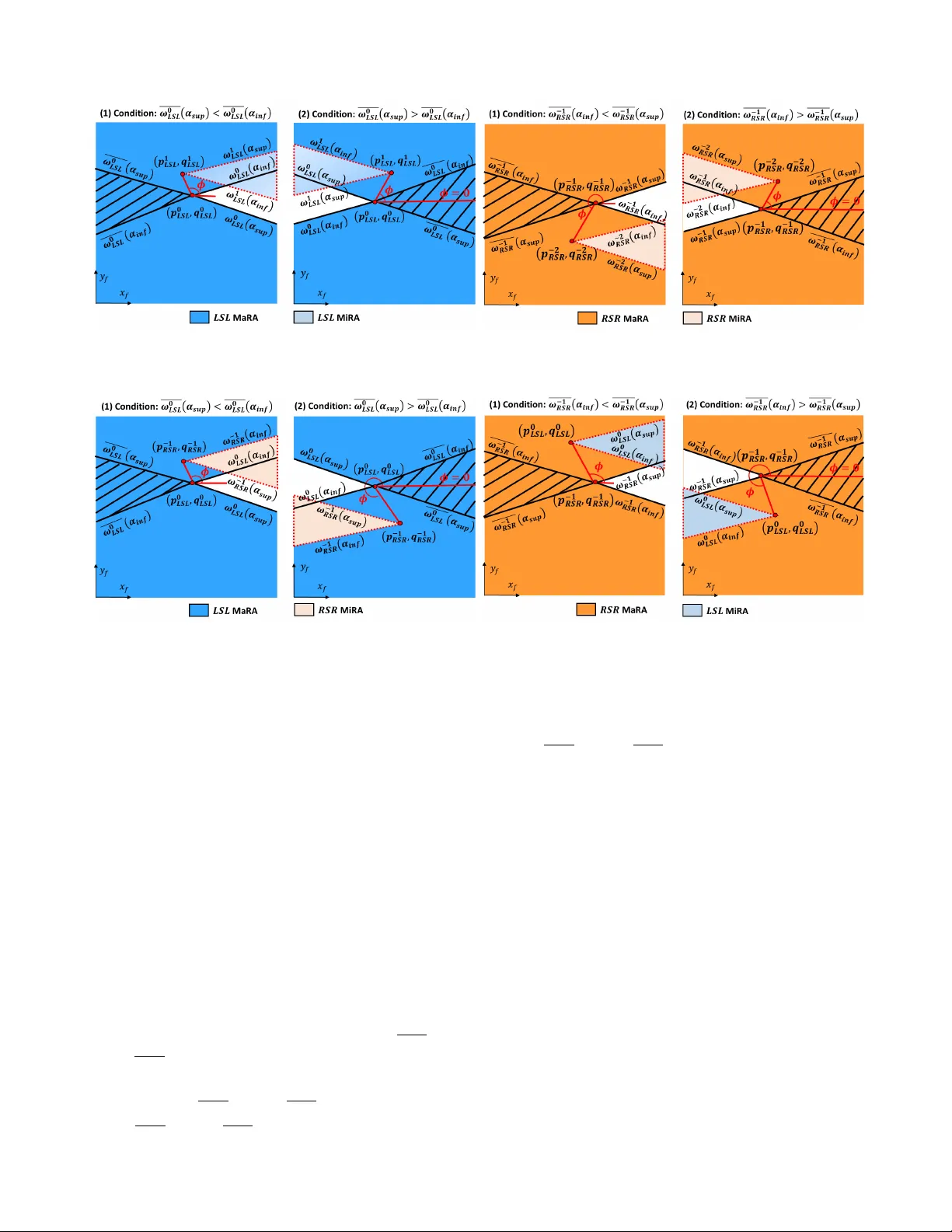
Robotics and Autonomous Systems Rapid P ath Planning for Dubins V ehicles under En vironmental Currents Khushboo Mittal † ∗ Junnan Song † ∗ Shalabh Gupta † ? Thomas A. W ettergren ‡ Abstract —This paper presents a rapid (real time) solution to the minimum-time path planning problem for Dubins vehicles under envir onmental currents (wind or ocean currents). Real- time solutions are essential in time-critical situations (such as replanning under dynamically changing envir onments or track- ing fast moving targets). T ypically , Dubins problem requires to solve for six path types; howe ver , due to the presence of currents, four of these path types require to solve the root-ﬁnding problem in volving transcendental functions. Thus, the existing methods result in high computation times and their applicability for real- time applications is limited. In this regard, in order to obtain a real-time solution, this paper proposes a novel approach where only a subset of two Dubins path types ( L SL and RS R ) are used which ha ve direct analytical solutions in the presence of currents. Howev er , these two path types do not provide full r eachability . W e show that by extending the feasible range of circular arcs in the LSL and RSR path types from 2 π to 4 π : 1) full reachability of any goal pose is guaranteed, and 2) paths with lower time costs as compared to the corresponding 2 π -arc paths can be produced. Theoretical properties ar e rigor ously established, supported by several examples, and evaluated in comparison to the Dubins solutions by extensive Monte-Carlo simulations. Index T erms —Dubins paths, path planning, envir onmental currents, curvatur e-constrained vehicles. L I S T O F S Y M B O L S v V ehicle velocity vector (m/s, m/s) v w Current velocity vector (m/s, m/s) v net Net velocity vector which is the vector sum of v and v w (m/s, m/s) w x , w y Components of v w along the x and y axes (m/s) θ V ehicle heading (rad) θ w Current heading (rad) u T urn rate (rad/s) r T urning radius (m) ( x 0 , y 0 , θ 0 ) Start pose (m, m, rad) ( x f , y f , θ f ) Goal pose (m, m, rad) k Feasible range parameter for an LSL or RSR path (-) ( p k LSL , q k LSL ) Center of rotation of the reachability ray for an LSL path and a giv en k (m, m) ( p k RSR , q k RSR ) Center of rotation of the reachability ray for an RSR path and a giv en k (m, m) This work was supported by US Ofﬁce of Nav al Research under A ward Number N000141613032. Any opinions or ﬁndings herein are those of the authors and do not necessarily reﬂect the views of the sponsoring agencies. ∗ These authors contributed equally to this work. † Department of Electrical and Computer Engineering, University of Connecticut, Storrs, CT 06269, USA. ‡ Nav al Undersea W arfare Center , Newport, RI 02841, USA. ? Corresponding Author (email id: shalabh.gupta@uconn.edu) α T urning angle of the ﬁrst arc of an L SL or RS R path (rad) α k in f [ su p ] Inﬁmum [supremum] of α for a given k (rad) β Length of the straight line segment of an LSL or RSR path (m) γ T urning angle of the last arc of an LSL or RSR path (rad) ω k LSL [ RSR ] ( α ) Rotation of a reachability ray for a giv en α and k for an LSL [ RS R ] path (rad) ω k LSL [ RSR ] ( α ) Rotation of ω k LSL [ RSR ] ( α ) by π (rad) φ k 1 , k 2 Rotation of the line segment joining the centers of rotation of two path types with parameters k 1 and k 2 , respectiv ely (rad) T T otal travel time (s) T 2 π [ 4 π ] T rav el time of the 2 π -arc [4 π -arc] path (s) T Dubins T rav el time of the optimal Dubins path (s) 1 . I N T R O D U C T I O N A. Backgr ound A fundamental problem in robotics is to ﬁnd the minimum- time path from a start pose to a goal pose while consider- ing several constraints on vehicles such as bounded curva- ture [1][2], bounded velocity [3][4] and bounded accelera- tion [5][6]. In particular , bounded curvature implies that the vehicle’ s turning is subject to a non-zero minimum turning radius corresponding to its speed and maximum turn rate. Dubins [7][8] used a geometrical approach to show that in absence of obstacles, the shortest path for a curv ature- constrained vehicle between a pair of poses must be one of the following six path types (also known as the Dubins curves): LSL , RSR , LSR , RSL , LRL and RLR , where L ( R ) refers to a left (right) turn with the maximum curvature, and S indicates a straight line segment. Since each path type is composed of three segments, it is uniquely determined by three path parameters, which describe the angles of the circular arcs and the length of the straight line segment. Recently , the authors proposed the T ? algorithm [9] which extended the Dubins approach to variable speed vehicles in obstacle-rich en vironments for time-optimal risk-aware motion planning. Howe ver , when environmental currents (e.g., wind or ocean currents) are present, the vehicle trajectory can be signiﬁcantly distorted [10], resulting in a minimum-time trajectory which is different from the minimum-distance trajectory . Along this line, the existing methods to compute the minimum-time trajectory for Dubins vehicles in the presence of en vironmental currents can be categorized into two types: 2 (a) 2 π -arc paths in the inertial frame (IF) and the current frame (CF). (b) 4 π -arc paths in the inertial frame (IF) and the current frame (CF). Figure 1: The minimum-time 2 π -arc paths vs. 4 π -arc paths. The current vector ( − 0 . 5 , 0 ) , the start pose ( 0 , 0 , 0 ) and the goal pose ( − 2 . 3 , 2 . 8 , π / 2 ) . (1) solutions in the inertial frame (IF) [11] and (2) solutions in the current frame (CF) [12][13]. The current frame is the inertial frame that moves at the speed and direction of the current. Fig. 1a shows the minimum-time Dubins path both in the IF and the CF . Due to the ef fect of current, the optimal Dubins path in the CF results in the distorted trochoidal path in the IF , therefore, the solutions in the IF hav e complex expressions [11]. A major adv antage of using the CF is that the effect of current on the vehicle trajectory is completely encompassed by the motion of the reference frame, hence the path planning problem can be simpliﬁed to a moving-tar get interception problem using Dubins paths [12][13][14][15]. While details are discussed later, Fig. 1b shows the optimal paths obtained by our method in the CF and the IF . B. The Real-time Challenge Although the abov e methods can produce the minimum- time trajectory for Dubins vehicles in the presence of static currents, their real-time application is limited due to their computational complexity . As shown in [11][13], the existing approaches require to solve for all six Dubins path types to ﬁnd the minimum-time trajectory . Out of these six path types, only LSL and RSR paths ha ve analytical solutions, while the re- maining four path types require to solve a root-ﬁnding problem in volving transcendental equations, which demand signiﬁcant computational efforts. Howe ver , in dynamic situations (e.g., changing currents, adaptive exploration [16][17] and target tracking [18]) it is critical to obtain a real-time solution for fast replanning, which is the focus of this paper . T o motiv ate this further, we generated the computation time required to obtain the minimum-time path from all six Dubins 50 60 70 80 90 100 110 120 Number of initial guesses 10 -4 10 -2 10 0 10 2 Computation time (s) All Dubins Paths Only LSL + RSR Paths Figure 2: Mean computation times for LSL and RSR paths as compared to all six Dubins paths, ov er 1000 randomly selected start and goal poses in a steady current environment, on a 2 . 4 GHz CPU computer with 8 GB RAM. path types, as shown in Fig. 2. Also, we compared this to the computation time required to get the minimum-time path from only the LSL and RSR path types. These computation times were obtained by av eraging ov er 1000 randomly selected start and goal poses in an environment with steady currents. The simulations were run in MA TLAB on a computer with 2 . 4 GHz CPU and 8 GB RAM. It is seen that using only LSL and RS R paths takes ∼ 6 . 4 × 10 − 4 s to get a solution. In contrast, using all six path types takes several orders of magnitude higher time to solve the transcendental equations. Furthermore, for practical applications, these numbers can become signiﬁcantly larger for less powerful on-board proces- sors. Moreover , these computation times depend on the non- linear solvers used. In addition, the implementation of these optimization solvers on on-board processors is challenging as compared to a system of equations with analytical solutions. Example : The potential implications of computation times are shown with an example. Consider an underwater vehicle moving at 2.5 m/s in an environment with a time-varying current with a speed of 2 m/s. No w , suppose the current changes direction towards that of the v ehicle motion, then a new path needs to be computed. Suppose that it takes ∼ 8 . 72 s for the on-board processor to get a solution using all six path types. Then, the vehicle would drift by a distance of 8 . 72 · ( 2 + 2 . 5 ) = 39 . 24 m before it could compute a new path. In comparison, if it uses only LS L and RSR path types, then this drift would be as little as 6 . 4 × 10 − 4 · ( 2 + 2 . 5 ) = 0 . 0029 m. Thus, computation time plays a crucial role in real-time path planning in dynamic environments. C. Our Appr oach Based on the above discussion, we propose a rapid (real- time) analytical solution as described below . 1) Proposed solution using 4 π -arc LSL and RSR paths : W e propose a solution in the CF using only the LSL and RSR path types. Howe ver , the limitation of using only this subset of path types is the lack of full reachability , i.e., they cannot reach ev ery goal pose in the presence of currents. T o overcome the abov e limitation, we propose a simple yet powerful technique. 3 Instead of using the regular LS L and RSR paths where the arc angles are within a range of [ 0 , 2 π ) , we propose to extend their arc range to [ 0 , 4 π ) [19]. Accordingly , we deﬁne the concepts of 2 π -arc and 4 π -arc paths below , where the parameters α ( γ ) and β refer to the turning angle of the ﬁrst (second) arc and the length of the straight line segment, respectiv ely . Deﬁnition 1 (2 π -arc Path ) . An L α S β L γ or R α S β R γ path is called a 2 π -ar c path, if α ∈ [ 0 , 2 π ) and γ ∈ [ 0 , 2 π ) . Deﬁnition 2 (4 π -arc Path ) . An L α S β L γ or R α S β R γ path is called a 4 π -ar c path, if α ∈ [ 0 , 4 π ) and γ ∈ [ 0 , 4 π ) . Remark 1. The six Dubins path types use the 2 π -arcs. Remark 2. It is shown that the 4 π -ar c LSL and RSR paths pr ovide full reac hability along with reduced total time costs as compar ed to the 2 π -arc LS L and RSR paths. Example : Figs. 1a and 1b sho w the minimum-time 2 π -arc and 4 π -arc paths, respecti vely , in both the IF and the CF . Fig. 1a sho ws the optimal 2 π -arc path, which is a RSR path with the total time cost of 20 . 91 s. In comparison, Fig. 1b shows the optimal 4 π -arc path, which is a LSL path with γ = 2 . 263 π > 2 π and the total time cost of 10 . 51 s. Intuitively , this happens because instead of tra veling against the current, the vehicle spends more time on arcs which allo ws the current to help it to reach the goal in less time. 2) Theoretical analysis of 4 π -arc LS L and RS R paths : W e present a rigorous theoretical analysis of the properties of 4 π -arc LS L and RSR paths. First, we dev elop a comprehensive procedure for reachability analysis of the 2 π -arc L SL and RSR paths. W e present the conditions for full reachability using these two path types with the support from Lemmas 1 − 4. The deriv ation of these conditions and the proofs of supporting lemmas are provided in Appendices A and B, respectiv ely . Next, it is numerically validated that the 2 π -arc LSL and RS R paths fail to satisfy the reachability conditions under all goal poses and current velocities. Thus, we present Theorem 1, which provides a guarantee of full reachability using 4 π - arc LSL and RSR paths. Further , it is established through Theorem 2 and Corollary 1, that the computational complexity of both 2 π -arc and 4 π -arc path solutions is the same. Along with pro viding full reachability , another important beneﬁt of 4 π -arc paths is their ability to generate faster , i.e., reduced time cost, paths in comparison to the 2 π -arc paths, which is highlighted in Theorem 3. Finally , Theorem 4 is presented to prov e that α , γ ∈ [ 0 , 4 π ) is sufﬁcient for optimality using LS L and RSR path types and thus further increasing of range is not needed. F or validation of our approach, extensiv e Monte Carlo simulations are performed to compare the performance of Dubins solutions and the proposed 4 π -arc path solutions. 3) Comparison of 4 π -arc L SL and RSR paths with Dubins : The solution obtained from the 4 π -arc LSL and RS R paths might be sub-optimal for certain goal poses as compared to the one obtained from the six Dubins path types; ho wev er , the longer con vergence time of the Dubins path solution might render it unsuitable for real-time applications. For ofﬂine applications in static current en vironments, one can use the Dubins path types to compute the minimum-time path. In this regard, Section 6-A provides a detailed compari- son of the solution quality (i.e., travel time cost) obtained for the 4 π -arc LSL and RSR solutions and the Dubins solutions. This analysis indicates that the advantage of the Dubins solutions ov er the 4 π -arc LSL and RS R solutions in terms of trav el time costs is not signiﬁcant. Furthermore, upon adding the computation time costs, the advantage of Dubins solutions is further reduced. On the other hand, for time critical real- time applications (e.g., target tracking, planning under moving obstacles, and changing currents), 4 π -arc paths provide rapid and reliable solutions without causing any vehicle drift. In contrast, the high computation times for Dubins solutions can cause vehicle drifts, thereby , resulting in longer sub-optimal trajectories which sometimes do not e ven conv erge to the goal pose. Section 6-E presents a comparativ e analysis in the presence of dynamic currents, which highlights the beneﬁts of the solutions obtained from the 4 π -arc LSL and RSR paths ov er the ones obtained from the six Dubins paths. D. Our Contributions The paper makes the following novel contributions: • Provides an analytical solution of the path planning prob- lem for Dubins vehicles under en vironmental currents, where the solution is based on a novel concept of 4 π -arc LSL and RSR paths and can be computed in real-time. In this regard, the paper presents the following: – A detailed analytical method to construct the reach- ability graphs of LS L and RS R paths. – A detailed deriv ation of the conditions under which 2 π -arc LSL and RSR paths provide full reachability . – A mathematical proof of full reachability of the 4 π - arc LSL and RS R paths under all conditions unlike the corresponding 2 π -arc paths ( Theorem 1 ). – A mathematical proof that a solution using 4 π -arc LSL and RSR paths can be obtained with the same computational workload as that needed for 2 π -arc paths ( Theorem 2 and Corollary 1 ), – A mathematical proof that 4 π -arc LS L and RSR paths provide reduced trav el time costs as compared to the corresponding 2 π -arc paths. ( Theorem 3 ). • Theoretical properties of 4 π -arc LSL and RS R paths are rigorously established and e valuated in comparison to Dubins solutions by extensiv e Monte-Carlo simulations. E. Or ganization The rest of the paper is organized as follows. Section 2 revie ws the existing literature. Section 3 presents the path planning problem and its analytical solution. Section 4 presents a detailed analytical procedure for the reachability analysis of the 2 π -arc LSL and RS R paths. Section 5 presents the theoreti- cal properties of 4 π -arc paths and shows their advantages over the 2 π -arc paths. Section 6 presents the comparati ve ev aluation results. Finally , the paper is concluded in Section 7 with rec- ommendations for future work. Appendices A and B provide proofs of reachability conditions and supporting lemmas. 4 2 . L I T E R AT U R E R E V I E W Recently , sev eral papers [20] hav e addressed the path plan- ning problem in the presence of currents. Garau et al. [21][22] studied the minimum-time path planning problem in marine en vironments with spatial current variability , where the time cost was deﬁned as the sum of step-wise costs that are speciﬁed by the trav eling distance over the v ehicle speed in the presence of ocean currents. Howe ver , the drawback in their design is that infeasible paths are penalized rather than being prohibited. Petres et al. [23] presented the FM ? algorithm to ﬁnd the minimum-time path for underwater vehicles, where the time cost is deﬁned over the inner product of the distance function and the current ﬁeld; howe ver , their cost function still penalizes rather than restricts infeasible paths. In this regard, Soulignac et al. [24] proposed a time cost function that projects the speed vector to both axes as opposed to taking its norm as in [22]. Accordingly , their method is restricted to feasible paths. In addition, energy based cost functions [25][26] have also been used for planning in the presence of ocean currents. Howe ver , the abov e-mentioned methods ignore any kine- matic motion constraints for v ehicles. Along this line, T echy and W oolsey [11] addressed the minimum-time path planning problem for a curvature-constrained vehicle in constant wind, based on the fact that the circular arcs are distorted by the wind into the trochoidal curves in the inertial frame. They deriv ed analytical solutions for LSL and RSR candidate paths, while for other paths of LSR , RSL , LRL and RLR , they must solv e certain transcendental equations to obtain solutions. Howe ver , as we show in Fig. 2, the root ﬁnding problem for transcendental equations can be computationally expensiv e. In contrast, McGee et al. [12] studied the minimum-time path planning problem in the current frame. They ﬁrst used Pontryagin’ s Minimum Principle to demonstrate that the op- timal path is comprised of straight line segments and curves of maximum turn rate. Then, they introduced the concept of a "virtual target" which starts at the goal state but mov es in the opposite direction as the wind. In this setup, the minimum- time problem is simpliﬁed into a target interception problem, where the objectiv e is to ﬁnd the earliest interception point in the current frame so that the Dubins path can meet with the virtual target in minimum time. Ho wev er , one must repeatedly check for the validity of possible interception points, which can be arbitrarily heavy to compute if the actual interception point lies far from the beginning search point. In this regard, Bakolas et al. [13] directly solved for the interception point in the current frame by introducing an extra parameter of interception time. They also showed that when the wind speed is less than the vehicle speed, the vehicle has full reachability , i.e., the optimal path always exists for any giv en goal pose. Howe ver , their solution methodology still inv olves solving for the roots of multiple transcendental equations, which could lead to heavy computational burden, thus prohibiting it from real-time applications. Some researchers used the Nonlinear T rajectory Generation (NTG) algorithm [27] based on spline curves to obtain the optimal trajectory of a glider with kinematic constraints in presence of dynamically varying ocean currents. The proposed algorithm relies on Sequential Quadratic Programming (SQP) approach to solve the nonlinear programming problem which might lead to sub-optimal solutions and high computational time. In comparison, this paper proposes a novel method which provides a rapid analytical solution to the path planning problem under currents with guaranteed full reachability . 3 . P R O B L E M D E S C R I P T I O N A N D S O L U T I O N This section presents the minimum-time path planning prob- lem for Dubins vehicles and its analytical solution. A. Pr oblem Description Consider a vehicle moving at a velocity v = ( v cos θ , v sin θ ) , where v ∈ R + is its speed and θ ∈ [ 0 , 2 π ) is its heading. A steady current is assumed to be present in the en vironment with v elocity v w = ( v w cos θ w , v w sin θ w ) ≡ ( w x , w y ) , where v w ∈ R + is its speed and θ w ∈ [ 0 , 2 π ) is its direction. The current speed is assumed to be slower than the vehicle speed, i.e., v w < v . Then, the motion of the vehicle can be described as:      ˙ x ( t ) = v · cos θ ( t ) + w x ˙ y ( t ) = v · sin θ ( t ) + w y ˙ θ ( t ) = u ( t ) , (1) where p = ( x , y , θ ) ∈ SE ( 2 ) is the vehicle pose and u indicates its turn rate. By choosing a proper unit, the vehicle speed can be normalized to v = 1. The turn rate u is symmetric and bounded, s.t., u ∈ [ − u max , u max ] , where u max ∈ R + is the maximum turn rate and the + / − sign indicates a left/right turn. These constraints imply that the vehicle is subject to the minimum turning radius of r = 1 / u max (for v = 1). Then, for a v ehicle operating in a current environment, as described in (1), the objective is to ﬁnd the minimum- time path from a start pose p st art = ( x 0 , y 0 , θ 0 ) to a goal pose p goal = ( x f , y f , θ f ) . The state-of-the-art solutions [11][12][13] to this problem require to solve for all six Dubins path types to ﬁnd the minimum-time path. Howe ver , as shown in (34) and (39) of [13], in order to obtain the path types of LSR , RSL , LRL and RLR , one must solve a root-ﬁnding problem in volving transcendental equations for numerical solutions. This inevitably requires signiﬁcant computation resources and thus can seriously restrict their usage in real-time applications. In this reg ard, in order to achie ve a real-time solution, we address the abo ve problem using only tw o path types which have direct analytical solutions. These are L α S β L γ and R α S β R γ , where α and γ are the turning angles of the ﬁrst and second arc segments, respectiv ely; and β ≥ 0 denotes the length of the straight line segment. Thus, the solution for each path type is uniquely determined by the 3-tuple { α , β , γ } of path parameters. Since these parameters can be solved analytically , the solution is obtained very fast (in real-time). Howe ver , due to using only a subset of the Dubins path types, there exist goal poses for which neither LS L nor RSR path can provide feasible solutions, i.e., LS L and RS R paths do not provide full reachability . T o address this issue, we extend the feasible ranges of α and γ from [ 0 , 2 π ) to [ 0 , 4 π ) . It is shown later that the extended LSL and RSR path types guarantee full reachability , and can provide the solutions with ev en less time costs. 5 (a) L α S β L γ path (b) R α S β R γ path Figure 3: Geometric illustration for LSL and RSR paths. B. Solutions for the LS L and RS R P aths This section deriv es the analytical solutions for the parame- ters of the LS L and RS R path types using the CF , which moves with the same speed and direction as that of the current. In the CF , the goal moves in the opposite direction with ( − w x , − w y ) . Thus, the problem is simpliﬁed to a moving-tar get interception problem. Therefore, the objecti ve is to ﬁnd the minimum interception time to meet with the moving goal using Dubins LSL and RS R paths. Without loss of generality , we choose the start pose ( x 0 , y 0 , θ 0 ) = ( 0 , 0 , 0 ) . 1) L α S β L γ P ath: As seen in Fig. 3a, in order to reach the goal ( x f , y f , θ f ) in the CF , the following boundary constraints must be satisﬁed for an LSL path [13]:          x f − w x T = r sin θ f + β cos α y f − w y T = r ( 1 − cos θ f ) + β sin α T =  r ( α + γ ) + β  / v α + γ = 2 k π + θ f , (2) where v = 1 and T ∈ R + is the total travel time. In addition, we introduce k ∈ Z to control the feasible ranges of α and γ . Speciﬁcally , for a 2 π -arc LSL path, since θ f ∈ [ 0 , 2 π ) and α , γ ∈ [ 0 , 2 π ) , one has k ∈ { 0 , 1 } . In contrast, for a 4 π -arc LSL path, since α , γ ∈ [ 0 , 4 π ) , one has k ∈ { 0 , 1 , 2 , 3 } . Note: W e show later that we need only k ∈ { 0 , 1 } to ﬁnd a feasible minimum-time 4 π -arc LS L path. Now , for a given k , deﬁne A k and B k as follows: ( A k = x f − r sin θ f − w x r ( 2 k π + θ f ) B k = y f − r ( 1 − cos θ f ) − w y r ( 2 k π + θ f ) , (3) which are constants that can be computed giv en the current velocity , and the start and goal poses. Then, using (2) and (3), we get: ( A k = β cos α + w x β B k = β sin α + w y β . (4) Based on (4), we can compute β by solving the quadratic equation  A k − w x β  2 +  B k − w y β  2 = β 2 , such that β = ± q ( A k w x + B k w y ) 2 + ( A k 2 + B k 2 )( 1 − v 2 w ) − ( A k w x + B k w y ) 1 − v 2 w . (5) It is seen from (5) that when v w < 1, β has valid solutions. Then, α can be computed as α = atan2  B k − β w y , A k − β w x  ( mod κ ) , (6) where κ = 2 π for 2 π -arc paths, and κ = 4 π for 4 π -arc paths. Thereafter , γ is computed as γ = 2 k π + θ f − α (mod κ ). 2) R α S β R γ P ath: As seen in Fig. 3b, the following bound- ary constraints must be satisﬁed for an RS R path:          x f − w x T = − r sin θ f + β cos α y f − w y T = − r ( 1 − cos θ f ) − β sin α T =  r ( α + γ ) + β  / v − α − γ = 2 k π + θ f . (7) For a 2 π -arc RS R path, since θ f ∈ [ 0 , 2 π ) and α , γ ∈ [ 0 , 2 π ) , one has k ∈ {− 1 , − 2 } ; while for a 4 π -arc RSR path, because α , γ ∈ [ 0 , 4 π ) , one has k ∈ {− 1 , − 2 , − 3 , − 4 } . Note: W e show later that we need only k ∈ {− 1 , − 2 } to ﬁnd a feasible minimum-time 4 π -arc RSR path. Now , deﬁne ( A k = x f + r sin θ f + w x r ( 2 k π + θ f ) B k = y f + r ( 1 − cos θ f ) + w y r ( 2 k π + θ f ) , (8) and using (7) and (8), we get: ( A k = β cos α + w x β B k = − β sin α + w y β . (9) Then, β is solved using  A k − w x β  2 +  B k − w y β  2 = β 2 , which results in the same expression as (5). Similarly , when v w < 1, β has valid solutions. Then, α can be computed as α = atan2 ( − B k + β w y , A k − β w x ) ( mod κ ) , (10) and γ is computed as γ = − 2 k π − θ f − α (mod κ ). C. F easible Ranges of P ath P arameters According to Defn. 1 and Defn. 2, the parameters α and γ are deﬁned over [ 0 , 2 π ) and [ 0 , 4 π ) for 2 π -arc paths and 4 π - arc paths, respectiv ely . Giv en the direction θ f ∈ [ 0 , 2 π ) of the goal pose, we can obtain tighter feasible ranges for α and γ . T able I shows the feasible ranges of path parameters for both 2 π -arc and 4 π -arc paths. An example is provided below . Example : Consider a 4 π -arc L SL path, where α ∈ [ 0 , 4 π ) and γ ∈ [ 0 , 4 π ) . There are four cases to study: • k = 0 (i.e., α + γ = θ f < 2 π ): Now , γ ≥ 0 = ⇒ α ≤ θ f . Similarly , α ≥ 0 = ⇒ γ ≤ θ f . Thus, the feasible range for both α and γ is [ 0 , θ f ] . • k = 1 (i.e., α + γ = 2 π + θ f < 4 π ): Again, γ ≥ 0 = ⇒ α ≤ 2 π + θ f . Similarly , α ≥ 0 = ⇒ γ ≤ 2 π + θ f . Thus, the feasible range for both α and γ is [ 0 , 2 π + θ f ] . 6 T able I: Feasible parameter ranges for 2 π -arc and 4 π -arc paths 2 π -arc Paths ( α , γ ranges are up to mod 2 π ) LSL Path T ype RSR Path T ype k α and γ β k α and γ β 0 [ 0 , θ f ] [ 0 , ∞ ) − 1 [ 0 , 2 π − θ f ] [ 0 , ∞ ) 1 ( θ f , 2 π ) [ 0 , ∞ ) − 2 ( 2 π − θ f , 2 π ) [ 0 , ∞ ) 4 π -arc Paths ( α , γ ranges are up to mod 4 π ) LSL Path T ype RSR Path T ype k α and γ β k α and γ β 0 [ 0 , θ f ] [ 0 , ∞ ) − 1 [ 0 , 2 π − θ f ] [ 0 , ∞ ) 1 [ 0 , 2 π + θ f ] [ 0 , ∞ ) − 2 [ 0 , 4 π − θ f ] [ 0 , ∞ ) 2 ( θ f , 4 π ) [ 0 , ∞ ) − 3 ( 2 π − θ f , 4 π ) [ 0 , ∞ ) 3 ( 2 π + θ f , 4 π ) [ 0 , ∞ ) − 4 ( 4 π − θ f , 4 π ) [ 0 , ∞ ) • k = 2 (i.e., α + γ = 4 π + θ f < 6 π ): Here γ < 4 π = ⇒ α > θ f . Similarly , α < 4 π = ⇒ γ > θ f . Thus, the feasible range for both α and γ is ( θ f , 4 π ) . • k = 3 (i.e., α + γ = 6 π + θ f < 8 π ): Here γ < 4 π = ⇒ α > 2 π + θ f . Similarly , α < 4 π = ⇒ γ > 2 π + θ f . Thus, the feasible range for both α and γ is ( 2 π + θ f , 4 π ) . Similarly , we can obtain the feasible range of path param- eters for 4 π -arc RS R path and for 2 π -arc LS L and RS R paths. 4 . R E A C H A B I L I T Y A N A L Y S I S O F 2 π - A R C P A T H S This section deriv es the analytical expressions for generat- ing the reachability graphs of 2 π -arc LSL and RS R path types and for ﬁnding the conditions of full reachability . A. Construction of Reachability Graphs First, we show that for a giv en α , the reachable goal points ( x f , y f ) lie on a ray . Then, we sho w that by v arying α , this ray rotates to form the reachability graph. • 2 π -arc LSL P aths: Let us denote p k LSL ≡ r sin θ f + w x r ( 2 k π + θ f ) , (11a) q k LSL ≡ r ( 1 − cos θ f ) + w y r ( 2 k π + θ f ) , (11b) which are constants for k ∈ { 0 , 1 } giv en θ f , w x and w y . Further , let us denote a ( α ) ≡ sin α + w y , (12a) c ( α ) ≡ cos α + w x . (12b) Then, using (3), (4), (11) and (12) we get: x f = p k LSL + β · c ( α ) , (13a) y f = q k LSL + β · a ( α ) . (13b) By performing a ( α ) · (13a) − c ( α ) · (13b), (13) is equiv alent to the following: Figure 4: Reachability region of the LS L path type obtained by anticlockwise rotation of (14) about the center of rotation ( p k LSL , q k LSL ) . a ( α ) x f − c ( α ) y f −  a ( α ) p k LSL − c ( α ) q k LSL  = 0 , s.t.: x f ≥ p k LSL , y f ≥ q k LSL , if a ( α ) ≥ 0 , c ( α ) ≥ 0 , x f < p k LSL , y f ≥ q k LSL , if a ( α ) ≥ 0 , c ( α ) < 0 , x f < p k LSL , y f < q k LSL , if a ( α ) < 0 , c ( α ) < 0 , x f ≥ p k LSL , y f < q k LSL , if a ( α ) < 0 , c ( α ) ≥ 0 . (14) The constraints in (14) are obtained by using the feasible range of β ≥ 0 in (13a) and (13b). As shown in Fig. 4, these constraints deﬁne the quadrants of the coordinate frame with center at  p k LSL , q k LSL  . F or a given α , (14) represents a reachability ray and the goal ( x f , y f ) is reachable if it lies on such ray . The rotation of (14), i.e., the angle it makes with the x-axis measured in the counterclockwise direction, is giv en as ω k LSL ( α ) = atan2  a ( α ) , c ( α )  ( mod 2 π ) , k ∈ { 0 , 1 } . (15) • 2 π -arc RSR Paths: Let us denote p k RSR ≡ − r sin θ f − w x r ( 2 k π + θ f ) , (16a) q k RSR ≡ − r ( 1 − cos θ f ) − w y r ( 2 k π + θ f ) . (16b) which are constants for k ∈ {− 1 , − 2 } given θ f , w x and w y . Further , let us denote b ( α ) ≡ sin α − w y . (17) Then, using (8), (9), (16) and (17) we get: x f = p k RSR + β · c ( α ) , (18a) y f = q k RSR − β · b ( α ) . (18b) By performing b ( α ) · (18a) + c ( α ) · (18b), (18) is equiv alent to the following: 7 Figure 5: An example showing the construction of reachability graph for 2 π -arc L SL and RSR path types. (a) MaRA for LSL with k = 0, (b) MiRA for L SL with k = 1, (c) union of MaRA and MiRA for LSL path, (d) MiRA for RSR with k = − 1, (e) MaRA for RSR with k = − 2, (f) union of MaRA and MiRA for RS R path, (f) complete reachability graph obtained by taking union of both L SL and RSR path types. b ( α ) x f + c ( α ) y f −  b ( α ) p k RSR + c ( α ) q k RSR  = 0 , s.t.: x f ≥ p k RSR , y f ≥ q k RSR , if b ( α ) ≤ 0 , c ( α ) ≥ 0 , x f < p k RSR , y f ≥ q k RSR , if b ( α ) ≤ 0 , c ( α ) < 0 , x f < p k RSR , y f < q k RSR , if b ( α ) > 0 , c ( α ) < 0 , x f ≥ p k RSR , y f < q k RSR , if b ( α ) > 0 , c ( α ) ≥ 0 . (19) The constraints in (19) are obtained by using the feasible range of β ≥ 0 in (18a) and (18b). Again, these constraints deﬁne the quadrants of the coordinate frame with center at  p k RSR , q k RSR  . For any given α , (19) represents a reachability ray , and the goal ( x f , y f ) is reachable if it lies on such ray . The rotation of (19) is giv en as ω k RSR ( α ) = atan2  − b ( α ) , c ( α )  ( mod 2 π ) , k ∈ {− 1 , − 2 } . (20) Now , we sho w a lemma that helps in constructing the reachability graphs using (14) and (19). Lemma 1. As α incr eases fr om α k in f to α k su p , then for: • L SL path type: r ay (14) rotates anticlockwise about the center  p k LSL , q k LSL  , ∀ k ∈ { 0 , 1 } . • RS R path type: ray (19) r otates clockwise about the center  p k RSR , q k RSR  , ∀ k ∈ {− 1 , − 2 } . Pr oof. See Appendix B1. Lemma 1 implies that the reachable area for LSL paths is obtained by rotating (14) about the center  p k LSL , q k LSL  , from ω k LSL ( α in f ) to ω k LSL ( α su p ) , where α k in f to α k su p are the bounds of α (see T able I) for a giv en k . Fig. 4 shows the reachable area for LSL paths obtained by this rotation. Note that there are dif ferent reachable areas for each k . Similarly , the reachable region for RS R paths is obtained by rotating (19) from ω k RSR ( α in f ) to ω k RSR ( α su p ) for both its k values. Remark 3. Note that for simplicity of notation, we omit the superscript of α whenever it is used in the ω function, wher e it assumes the superscript of ω . For further explanation, we introduce the concepts of Major Reachable Ar ea (MaRA) and Minor Reachable Area (MiRA). Deﬁnition 3 ( MaRA ) . F or an LSL (RSR) path type, MaRA is the larg er of the r eachable areas spanned by k = 0 or 1 (k = − 1 or − 2 ). Deﬁnition 4 ( MiRA ) . F or an LSL (RSR) path type, MiRA is the smaller of the reac hable areas spanned by k = 0 or 1 (k = − 1 or − 2 ). Example : Fig. 5 shows an example of the construction of the reachability graph for 2 π -arc LSL and RS R path types. Here, the en vironment has a current of speed v w = 0 . 5 m/s and direction θ w = π / 3. The goal pose has the heading angle θ f = 7 π / 4, while its position ( x f , y f ) is varied within [ − 10 , 10 ] . Figs. 5a and 5b show the MaRA ( k = 0) and MiRA ( k = 1) 8 (a) 3D reachable space for different parameters (b) v w = 0 . 25 (c) v w = 0 . 75 Figure 6: The parameter space between θ f ∈ [ 0 , 2 π ) , θ w ∈ [ 0 , 2 π ) and v w = ( 0 , 1 ) , where full reachability is achieved. of the LSL paths, respectiv ely , which are obtained by rotating the ray (14) by varying α from α k in f to α k su p . The corre- sponding centers of rotation ( p 0 LSL , q 0 LSL ) = ( 0 . 67 , 2 . 67 ) and ( p 1 LSL , q 1 LSL ) = ( 2 . 24 , 5 . 39 ) are also shown. Fig. 5c sho ws the total reachable area of the LSL paths obtained by combining the MaRA and MiRA from Figs. 5a and 5b, respectively . Clearly , the LS L paths do not provide full reachability . Similarly , Figs. 5d and 5e show the MiRA ( k = − 1) and MaRA ( k = − 2) of the RSR paths, respectiv ely , which are obtained by rotating the ray (19) by varying α from α k in f to α k su p . The corresponding centers of rotation ( p − 1 RSR , q − 1 RSR ) = ( 0 . 90 , 0 . 05 ) and ( p − 2 RSR , q − 2 RSR ) = ( 2 . 47 , 2 . 77 ) are also shown. Again, Fig. 5f shows the total reachable area of the RS R path obtained by combining the MaRA and MiRA from Figs. 5d and 5e, respecti vely . As seen, the RSR paths also do not provide full reachability . Finally , Fig. 5g shows the complete reachability graph using both LS L and RS R path types, which is obtained by combining Figs. 5c and 5f. As seen in Fig. 5g, there is still some region that is unreachable, thus both L SL and RSR path types together also do not provide full reachability . B. Full Reachability Conditions for the 2 π -arc P ath T ypes After acquiring the analytical expressions for generating the reachability graphs of the 2 π -arc LS L and RSR path types, we now in vestigate the conditions under which these paths pro vide full reachability . Note that full reachability is achiev ed if the entire space is cov ered by atleast one of the following combinations: 1) Union of MaRA and MiRA of LSL , and/or 2) Union of MaRA and MiRA of RSR , and/or Figure 7: The optimal 4 π -arc paths in the IF and CF , while there is no feasible solution for 2 π -arc paths. The start pose ( x 0 , y 0 , θ 0 ) = ( 0 , 0 , 0 ) and the goal pose ( x f , y f , θ f ) = ( 6 , 3 , 7 π / 4 ) . The optimal 4 π -arc path parameters are: α = 0 . 116 π , β = 2 . 976, γ = 2 . 135 π . 3) Union of MaRA of L SL and MiRA of RSR , and/or 4) Union of MaRA of RS R and MiRA of LSL . Remark 4. W e show by Lemma 4 in Appendix A that these four cases are sufﬁcient for r eachability analysis. For continuity of reading, the deriv ations of the full reach- ability conditions for the abov e four cases are presented in Appendix A and the results are summarized in T able III. If at some goal pose, all of the conditions in T able III are violated, then it is unreachable by 2 π -arc paths. Next, we visually v erify the unreachable regions using a numerical validation. Numerical V alidation : The reachabilty conditions for 2 π - arc paths are shown in the last column of T able III in Appendix A. These reachability conditions only depend on parameters θ f , θ w and v w . Thus, we construct a 3D reachability graph by varying θ f ∈ [ 0 , 2 π ) and θ w ∈ [ 0 , 2 π ) in steps of π / 100, and v w ∈ ( 0 , 1 ) in steps of 0 . 1. For any 3D parametric point, if at least one of the full reachability conditions is satisﬁed, then such point is colored, and the color varies with respect to v w , as shown in Fig. 6a. In contrast, the white area indicates the parametric space where all the reachability conditions are violated, i.e., providing no feasible solutions. This validation illustrates that full reachability is not achieved by 2 π -arc LSL and RSR paths. Figs. 6b and 6c show the cross sections of Fig. 6a at v w = 0 . 25 m/s and v w = 0 . 75 m/s, respectiv ely . It is seen that a higher v w leads to a smaller reachable space. Fig. 7 shows a speciﬁc example where 2 π -arc path does not exist, but 4 π -arc path does. The start pose ( x 0 , y 0 , θ 0 ) = ( 0 , 0 , 0 ) , the goal pose ( x f , y f , θ f ) = ( 6 , 3 , 7 π / 4 ) , and the current mov es at speed v w = 0 . 5 m/s in the direction of θ w = π / 3. It is seen that the turning angle of the second turn in the optimal 4 π -arc path has γ = 2 . 135 π > 2 π , which drives the vehicle to circle around at the end so that it can meet with the exact goal heading with the help of external current. 9 (a) Reachability graphs of the 2 π -arc paths for θ f = 5 π / 4 and 7 π / 4. (b) Reachability graphs of the 4 π -arc paths for θ f = 5 π / 4 and 7 π / 4. Figure 8: An example of reachability graphs for the 2 π -arc and 4 π -arc paths. The dominant of the LS L (blue color) or RSR (orange color) paths is shown in the corresponding area. White color indicates unreachable area. 5 . T H E O R E T I C A L P RO P E RT I E S O F 4 π - A R C P A T H S The previous section established that 2 π -arc LSL and RSR paths do not guarantee full reachability . This section presents the theoretical properties of 4 π -arc paths which highlight their advantages over 2 π -arc paths in terms of: 1) full reachability , and 2) lower time costs, while requiring similar computational complexity . First, we present the concept of a dominant path type and show an example to motiv ate the above properties. Deﬁnition 5 ( Dominant Path T ype ) . F or a given goal pose, a path type LSL (RSR) is said to be dominant over RSR (LS L), if it achieves a lower time cost to reac h that goal pose. Example : Figs. 8a and 8b present the reachability plots of 2 π -arc and 4 π -arc paths, respectiv ely . These are generated for an en vironment which has a current of speed v w = 0 . 5 m/s and heading angle θ w = π / 3. The coordinates of the goal pose ( x f , y f ) are varied within [ − 10 , 10 ] . The two subplots of each ﬁgure correspond to two different goal pose directions θ f ∈ { 5 π / 4 , 7 π / 4 } . A region is color-coded cyan (orange) if an LSL ( RS R ) path exists and dominant over the RSR ( L SL ) path type. The white color indicates that no feasible solution exists for either path type and the region is unreachable. As seen in Fig. 8a(2), for θ f = 7 π / 4, there exists a region which is unreachable for 2 π -arc paths. This implies that for any goal pose inside this region, no solutions exist for α and γ within their feasible ranges deﬁned in T able I. In contrast, as seen in Fig. 8b(2), 4 π -arc paths achieve full reachability . Furthermore, the dominant path type (i.e., LS L or RS R ) for the same region could be different when using the 2 π - arc paths and 4 π -arc paths, as seen in Figs. 8a(1) and 8b(1) corresponding to θ f = 5 π / 4. Since 4 π -arc solutions already include the 2 π -arc solutions, the above observation implies that there exist goal poses for which 4 π -arc paths can achiev e ev en lower time costs as compared to the 2 π -arc paths. Roadmap of this Section: In the follo wing subsections, we present four theorems to highlight the theoretical properties of 4 π -arc LSL and RS R paths and compare them with the corresponding 2 π -arc paths. First, Theorem 1 proves that both the LS L and RSR 4 π -arc paths provide full reachability unlike the 2 π -arc paths. Then, Theorem 2 and Corollary 1 show that the computation workload required to get a solution using the 4 π -arc paths is the same as that using the 2 π -arc paths. Next, Theorem 3 compares the optimality of 4 π -arc and 2 π -arc path solutions and shows that the optimal trajectory provided by 4 π -arc paths is either of shorter time or same as that provided by 2 π -arc paths. Finally , Theorem 4 proves that α , γ ∈ [ 0 , 4 π ) is suf ﬁcient for optimality and increasing the range of these arc segments beyond 4 π does not lead to a shorter time path. A. Full Reachability of 4 π -ar c P aths The following theorem relates to the reachability of the 4 π - arc solutions for the L SL and RSR path types. Theorem 1 ( Full reachability of 4 π -arc paths ) . The 4 π -arc LSL and RSR paths individually pr ovide full r eachability . Pr oof. Full reachability implies the existence of solution for any goal pose. W e prov e for L SL and RSR paths below . • 4 π -arc LSL paths : Consider k = 1. From T able I, α in f = 0 and α su p = 2 π + θ f > 2 π . Using Lemma 1, we construct the reachable space for k = 1 by rotating the ray (14) around ( p 1 LSL , q 1 LSL ) by varying α from 0 to 2 π + θ f . In this process, the ray (14) swipes in the anticlockwise direction from ω 1 LSL ( 0 ) to ω 1 LSL ( 2 π + θ f ) . Howe ver , when α reaches 2 π < 2 π + θ f , the rotation of ray (14) becomes ω 1 LSL ( 2 π ) = ω 1 LSL ( 0 ) = atan2 ( w y , 1 + w x ) ( mod 2 π ) , which implies that the ray comes back to the start again and continues swiping thereafter . This means that for k = 1, the whole space is cov ered and full reachability is ob- tained. Now consider k = 2. From T able I, α in f = θ f and α su p = 4 π . F ollowing the same process as for the k = 1 case, one can see that the swiped area for k = 2 also cov ers the whole area and full reachability is obtained. In summary , 4 π -arc LS L paths guarantee full reachability . (Note: for k = 0 and 3, the swiped area does not cover the whole space, hence they do not provide full reachability .) • 4 π -arc RSR paths : Consider k = − 2. From T able I, α in f = 0 and α su p = 4 π − θ f > 2 π . Using Lemma 1, as α gro ws, the ray (19) rotates around ( p − 2 RSR , q − 2 RSR ) in the clockwise direction from ω − 2 RSR ( 0 ) to ω − 2 RSR ( 4 π − θ f ) . During this process, when α reaches 2 π < 4 π − θ f , the rotation of ray (19) becomes ω − 2 RSR ( 2 π ) = ω − 2 RSR ( 0 ) = atan2 ( w y , 1 + w x ) ( mod 2 π ) , which implies that it comes back to the start again and continues swiping thereafter . This means that for k = − 2, the whole space is covered and full reachability is obtained. No w consider k = − 3. From T able I, α in f = 2 π − θ f and α su p = 4 π . Following the same process as for the k = − 2 case, one can see that 10 the swiped area for k = − 3 also covers the whole space and full reachability is obtained. In summary , 4 π -arc RSR paths guarantee full reachability . (Note: for k = − 1 and − 4, the swiped area does not cover the whole space, hence they do not provide full reachability .) Hence proved. B. T ime Costs of 4 π -ar c LSL and RSR P aths Now , we analyse the time costs of 4 π -arc LSL and RSR paths and compare them to the corresponding 2 π -arc paths. Based on (2) and substituting v = 1, the time cost for an LSL path type is giv en as T = r ( α + γ ) + β = 2 k π r + r θ f + β . (21) Similarly , based on (7), the time cost for an RS R path type is giv en as T = r ( α + γ ) + β = − 2 k π r − r θ f + β . (22) From this point on, let us denote T k and β k as the values of T and β for a given k , i.e., T k = 2 k π r + r θ f + β k for an LSL path and T k = − 2 k π r − r θ f + β k for an RSR path. Theorem 2. The following are true: • T 0 < T 1 < T 2 < T 3 , for 4 π -ar c LSL paths. • T − 1 < T − 2 < T − 3 < T − 4 , for 4 π -ar c RSR paths. Pr oof. Let us denote ∆ T k as the difference in time cost T k between two consecutiv e k values, i.e., for L SL path type, ∆ T k , T k + 1 − T k = 2 π r + β k + 1 − β k , k = 0 , 1 , 2 , (23) and for RSR path type, ∆ T k , T k − 1 − T k = 2 π r + β k − 1 − β k , k = − 1 , − 2 , − 3 . (24) Consider 4 π -arc LSL paths. T o prove the theorem, we show that ∆ T k > 0 , ∀ k = 0 , 1 , 2. Fig. 9a sho ws the feasible 4 π -arc LSL paths in the CF , corresponding to k (shown in solid blue) and k + 1 (sho wn in solid red), to reach the goal pose ( x f , y f , θ f ) . These paths hav e the time costs T k and T k + 1 , respectiv ely . While these two paths share the same start pose, due to dif ferent trav el times, the corresponding goal poses in the CF become G k = ( x f − w x T k , y f − w y T k , θ f ) and G k + 1 = ( x f − w x T k + 1 , y f − w y T k + 1 , θ f ) , where k G k + 1 − G k k = q w 2 x ∆ T 2 k + w 2 y ∆ T 2 k = v w | ∆ T k | . Since an LS L path is comprised of an α arc, a straight line and a γ arc, one can equi valently combine the two arcs followed by the straight line to reach the same goal pose, as shown by the dotted line paths in Fig. 9a, corresponding to k (shown in dotted blue) and k + 1 (shown in dotted red). According to (2), α + γ = 2 k π + θ f , so if k is increased by 1, it adds a full 2 π rotation to this combined α and γ arc. This implies that after combining these arcs, the blue and red dotted straight lines share the same start point O k ∈ R 2 . Note that the solid straight lines are parallel to the corresponding dotted straight lines, with lengths β k and β k + 1 , respectiv ely . (a) LSL path type (b) RSR path type Figure 9: Illustrative ﬁgures to show ∆ T k > 0 , ∀ k in Theorem 2. Now consider the triangle formed by O k , G k and G k + 1 , shown by the shaded region in Fig. 9a, where k O k − G k k = β k and k O k − G k + 1 k = β k + 1 . Next, we consider three cases: 1) ∆ T k > 0: In this case, k G k + 1 − G k k = v w ∆ T k . Using the triangle inequalities, we get | β k + 1 − β k | < v w ∆ T k . By (23), β k + 1 − β k = ∆ T k − 2 π r . Hence, | ∆ T k − 2 π r | < v w ∆ T k = ⇒ 2 π r 1 + v w < ∆ T k < 2 π r 1 − v w . Note that if O k , G k and G k + 1 fall on one line, then | β k + 1 − β k | = v w ∆ T k , then ∆ T k = 2 π r 1 + v w or 2 π r 1 − v w . Therefore, the feasible range of ∆ T k is ∆ T k ∈  2 π r 1 + v w , 2 π r 1 − v w  . (25) 2) ∆ T k < 0: In this case, k G k + 1 − G k k = − v w ∆ T k . Then, based on the triangle inequalities, | β k + 1 − β k | < − v w ∆ T k . Again substituting β k + 1 − β k = ∆ T k − 2 π r from (23), we get 2 π r 1 − v w < ∆ T k < 2 π r 1 + v w . Howe ver , since 0 < v w < 1, this inequality is in valid. Thus, ∆ T k < 0 is impossible. 3) ∆ T k = 0: In this case, k G k + 1 − G k k = 0. Then, | β k + 1 − β k | = 0 = ⇒ ∆ T k − 2 π r = 0 = ⇒ ∆ T k = 2 π r , which is a contradiction, hence ∆ T k = 0 is impossible. Thus, ∆ T k > 0 , ∀ k , and its bounds are given in (25). Simi- larly , for 4 π -arc RSR paths, the bounds of ∆ T k can be deriv ed using Fig. 9b, leading to the same bounds and the deriv ation is omitted here. Hence proved. The following corollary shows that in order to obtain the minimum-time solutions using 4 π -arc paths, it is sufﬁcient to use k = { 0 , 1 } for LSL path type and k = {− 1 , − 2 } for RSR path type and the remaining k values are not needed. Corollary 1. A minimum-time solution for the 4 π -ar c paths can be obtained by using • k ∈ { 0 , 1 } for LSL paths and • k ∈ {− 1 , − 2 } for RSR paths. Pr oof. Theorem 2 implies that based on time costs, the pre- ferred solutions follo w the order k = 0 , 1 , 2 , 3 for LSL paths and k = − 1 , − 2 , − 3 , − 4 for RS R paths. Theorem 1 suggests that 11 for LSL paths, k = 0 solutions do not provide full reachability; howe ver full reachability can be achieved by k = 1 solutions. Similarly , for RSR paths, k = − 1 solutions do not provide full reachability; howe ver full reachability can be achiev ed by k = − 2 solutions. Thus, in order to get full reachability and to obtain minimum-time paths, one must solve only for k ∈ { 0 , 1 } for L SL paths, and k ∈ {− 1 , − 2 } for RSR paths. Hence proved. Remark 5. Cor ollary 1 implies that the computation workload r equir ed to get a solution using the 4 π -ar c paths is the same as that using the 2 π -arc paths. Corollary 2. A minimum-time 4 π -ar c LSL or RSR solution must satisfy α + γ < 4 π . Pr oof. Using Corollary 1 and that θ f < 2 π , substitute k = 1 into (2) and k = − 2 into (7), one can easily get the result. Hence proved. Remark 6. As seen fr om T able I, the feasible r anges of parameters α and γ for the 4 π -arc L SL (RSR) paths for k = 0 (k = − 1 ) ar e the same as those of the corr esponding 2 π -arc paths. However , for k = 1 (k = − 2 ), the parameter ranges for 4 π -ar c LSL (RSR) paths form supersets of the corresponding ranges of the 2 π -arc paths. Theorem 3. The time costs of 4 π -arc path solutions ar e lower than or same as those of the 2 π -arc path solutions. Pr oof. First, consider the case when both 2 π -arc LS L and RSR solutions exist for a gi ven goal pose. Remark 6 indicates that any valid 2 π -arc path solution is also a valid 4 π -arc path solution. Hence, in this case the time cost of 4 π -arc path solution is the same as that of the 2 π -arc path solution. Second, consider the case when neither of the 2 π -arc LSL and RSR solutions exist for a given goal pose. In this case, Theorem 1 guarantees that 4 π -arc LSL and RS R solutions exist for that goal pose. Third, consider the case when only one of the 2 π -arc LSL or RS R path solution exists for a giv en goal pose, i.e., the other path type does not provide a solution. Thus, the dominant solution is the only existing path type. Howe ver , from Theorem 1, for 4 π -arc paths both LS L and RSR paths exist and the dominant solution is selected from these two path types with the minimum time cost. Thus, due to the existence of an extra solution provided by the 4 π -arc paths, the time cost of the dominant path could be better than or same as that of the single solution provided by the 2 π -arc paths. The examples below validate this case. Hence prov ed. Example : W e show an example where the 4 π -arc paths provide faster (i.e., lower time cost) solutions as compared to the 2 π -arc paths. W e ﬁrst construct the time cost map for a ﬁxed set of θ f , v w and θ w , where each ( x f , y f ) is assigned the time cost of the dominant path between LS L and RS R paths. Fig. 10 sho ws the example generated for an en vironment with current of v w = 0 . 5 m/s and θ w = π . For constructing the time cost map, the goal poses are v aried within x f , y f ∈ [ − 10 , 10 ] m with a ﬁx ed heading angle θ f = π / 4. Figs. 10a (a) Cost map of 2 π -arc paths. (b) Cost map of 4 π -arc paths. Start Goal 2 -arc path: 24.47 s 4 -arc path: 13.21 s 2 -arc path (IF) 4 -arc path (IF) 2 -arc path (CF) 4 -arc path (CF) Moving direc on of the goal in CF Current Time Cost (c) The 2 π -arc and 4 π -arc path solutions in the IF and CF . The start pose ( x 0 , y 0 , θ 0 ) = ( 0 , 0 , 0 ) and the goal pose ( x f , y f , θ f ) = ( − 1 , 4 , π / 4 ) . The optimal 2 π -arc path has: α = 1 . 890 π , β = 12 . 691 and γ = 1 . 860 π ; and the optimal 4 π -arc path has: α = 0 . 206 π , β = 6 . 143 and γ = 2 . 044 π . Figure 10: An example to illustrate the result of Theorem 3 that the 4 π -arc paths provide faster solutions than the 2 π -arc paths. and 10b show the time cost maps for 2 π -arc paths and 4 π -arc paths, respectiv ely . The color code indicates the value of the time cost. Clearly , there exist many goal poses where 4 π -arc paths provide signiﬁcantly lower time costs. Next, we pick a goal pose where 4 π -arc paths provide a lower time cost, say ( x f , y f , θ f ) = ( − 1 , 4 , π / 4 ) . Then, we draw the optimal 2 π -arc and 4 π -arc paths in the IF and the CF , as shown in Fig. 10c. The 2 π -arc path follows the RSR path type, and requires a total time cost of 24 . 47 s. In comparison, the 4 π -arc path follows the LSL path type and the total time cost is reduced to 13 . 21 s. This is because on the 2 π -arc path, the vehicle has to travel a longer straight-line segment that is almost in an opposite direction to the current, hence its actual speed in the inertial frame becomes slower . On the other hand, the 4 π -arc path ﬁrst makes a small left turn, followed by a much shorter straight-line segment; then, it starts circling for ov er 2 π while letting the current help it to reach the goal. Theorem 4. The time cost T cannot be reduced further by extending the ranges of ar c se gments ( α and γ ) over 4 π . Pr oof. Suppose the ranges of α and γ are deﬁned over [ 0 , 2 n π ) , where n > 2 and n ∈ N + . Then, using the same procedure as described in Section 3-B, we get a larger set of feasible values of k , s.t. for LS L paths, k ∈ { 0 , 1 , . . . , 2 n − 1 } , and for RSR paths, k ∈ {− 1 , − 2 , . . . , − 2 n } . Then, one can deriv e the feasible ranges for α and γ . Con- 12 sider a 2 n π -arc LSL path, where α ∈ [ 0 , 2 n π ) and γ ∈ [ 0 , 2 n π ) . W e examine only k = 0 , 1 cases as necessary . • k = 0 (i.e., α + γ = θ f < 2 π ): Now , γ ≥ 0 = ⇒ α ≤ θ f . Similarly , α ≥ 0 = ⇒ γ ≤ θ f . Thus, the feasible range for both α and γ is [ 0 , θ f ] . • k = 1 (i.e., α + γ = 2 π + θ f < 4 π ): Again, γ ≥ 0 = ⇒ α ≤ 2 π + θ f . Similarly , α ≥ 0 = ⇒ γ ≤ 2 π + θ f . Thus, the feasible range for both α and γ is [ 0 , 2 π + θ f ] . The above analysis indicates that for 2 n π -arc LSL paths, if n > 2, the feasible ranges of α and γ for k = 0 , 1 are the same to the corresponding ones for 4 π -arc LSL paths, as presented in T able I. Similarly , one can verify that for 2 n π -arc RS R paths, if n > 2, the feasible ranges of α and γ for k = − 1 , − 2 are also the same to the corresponding ones for 4 π -arc RSR paths. Since the feasible ranges of α and γ for 2 n π -arcs are the same as those for 4 π -arc paths, by Theorem 1 full reachability is achieved using k = 0 , 1 for LSL paths and k = − 1 , − 2 for RSR paths. Further , by Theorem 2, ∆ T k > 0 , ∀ k . Therefore, for n > 2, we only need to search over k = 0 , 1 for LSL paths and k = − 1 , − 2 for RS R paths to get the minimum-time path. This implies that the time cost T is not reduced by extending the feasible ranges of α and γ ov er 4 π . Hence prov ed. 6 . R E S U LT S A N D D I S C U S S I O N This section presents the results of the proposed approach, which uses the 4 π -arc LS L and RS R paths, in comparison to the Dubins approach, which uses the six 2 π -arc paths. W e discuss the performance of these two approaches ﬁrst in an en vironment with static current and then in an en vironment with dynamically changing current. W e conduct Monte Carlo simulations as needed for statistical performance ev aluation. The simulations were done on a computer with 2 . 4 GHz and 8 GB RAM. In order to obtain a solution using the Dubins approach, the transcendental functions are solved using the function fsolve in MA TLAB. On average, the Dubins approach took ∼ 8 . 72 s to get a solution with 100 initial guesses, while the 4 π -arc paths approach took only ∼ 0 . 64 ms which is orders of magnitude faster than that of the Dubins computation. A. Comparison of 4 π -arc LS L and RSR solutions with Dubins solutions in a static current envir onment First, we considered an en vironment with a static current where the planning is done ofﬂine. This comparative study is presented using two metrics: a) the solution quality (i.e., the trav el time cost) and b) the total time cost (i.e., the of ﬂine computation time cost plus the trav el time cost). Simulation Setup : The start pose is ﬁxed at ( x 0 , y 0 , θ 0 ) = ( 0 , 0 , 0 ) . Then, 80 dif ferent goal positions are distrib uted uniformly on the boundaries of concentric squares at a distance of R = { 5 , 10 , 50 , 100 , 200 } m around the origin. For each goal position, 6 different heading angles θ f ∈ { m π 3 , m = 0 , . . . 5 } are considered. This leads to a total of 480 goal poses. The vehicle and current speeds are taken to be v = 1 m/s and v w = 0 . 5 m/s, respectively , where 6 different current heading angles θ w ∈ { m π 3 , m = 0 , . . . 5 } are considered, thus leading to a total number of 2880 runs. (a) Savings in travel time: T Dubins - T 4 π . (b) Savings in total time after including computation time. Figure 11: Time savings of the 4 π -arc solutions w .r .t. the Dubins solutions over 2880 different simulation runs in a static current en vironment. For each run, the trav el time cost and computation time cost are obtained for the two approaches. Fig 11 shows the savings obtained with the proposed 4 π -arc path solutions as compared to the Dubins solutions. Fig 11a shows the savings in trav el time, computed as T Dubins - T 4 π , where T Dubins and T 4 π refer to the travel time costs of Dubins paths and 4 π -arc paths, respecti vely . As seen in the ﬁgure, in more than 50% of the cases, the trav el time costs of 4 π -arc path solutions match those of the Dubins solutions. Although the performance of Dubins paths is better than the 4 π -arc paths for the remaining cases, the travel time cost difference is not that signiﬁcant. Fig. 11b sho ws the total time cost obtained by adding the computation time costs taken by the two approaches to their respectiv e trav el time costs. It is seen that in more than 90% of the cases the total time of the 4 π -arc solutions is lower than that of the Dubins solutions; thus, 4 π -arc solutions yield a superior performance upon considering the computation times. Based on these trends, it is observed that although Du- bins solutions are suitable for applications requiring ofﬂine planning, they do not provide signiﬁcant advantage over the 4 π -arc LSL and RS R solutions in terms of travel time costs. Furthermore, when computation times are added then Dubins solutions provide worse total time costs in a signiﬁcant majority of cases. Moreov er , as discussed in Section 6-E, for applications requiring online planning in dynamic current en vironments, the high computation times of Dubins solutions cause signiﬁcant vehicle drifts, thus, resulting in longer sub- optimal trajectories which sometimes do not even con ver ge to the goal pose. In such situations, 4 π -arc paths lead to faster and reliable solutions with negligible drifts allowing the vehicle to reach the goal pose precisely in shorter times. B. Effect of a Change in Curr ent During path e xecution, a change in the current’ s speed or heading could deviate the vehicle from its original path if left unattended. Hence, it is necessary to replan online upon detection of a change in current. Howe ver , as explained in Section 1, using Dubins solution to regenerate the path to reach the goal pose requires considerable amount of computation time to solve the transcendental functions, during which the vehicle can drift noticeably . In particular , the vehicle drift would be along the direction of the net velocity of the vehicle 13 (a) An example of path replanning under changing current. Start pose ( x 0 , y 0 , θ 0 ) = ( 0 , 0 , 0 ) and goal pose ( x f , y f , θ f ) = ( 5 , 8 . 5 , 3 π / 4 ) . Initially , the current has v w = 0 . 5 m/s and θ w = π , which changed at time 3 . 2 s to a new current with v w = 0 . 75 m/s and θ w = 3 π / 2. The radius of precision circle is 1 m. (b) An example to show the effect of the net velocity of the vehicle drift. Start pose ( x 0 , y 0 , θ 0 ) = ( 0 , 0 , 0 ) and goal pose ( x f , y f , θ f ) = ( 5 , 8 . 5 , 3 π / 4 ) . Initially , the current has v w = 0 . 5 m/s and θ w = 3 π / 2, which changed at time 3 . 72 s to a new current. Figure 12: Illustrative examples of replanning under changing current, and the effect of v net on the vehicle drift. and the current at that moment. T o account for such drifts, the replanning is done by using a predicted position of the vehicle after the drift as the new start pose. This predicted position is computed by adding a translation (i.e., the product of the av erage computation time of ∼ 8 . 72 s and the net velocity) to the vehicle pose. Note that the predicted position is needed only for the Dubins solution, while it is unnecessary for the 4 π -arc path solution due to its negligible computation time. The vehicle is considered to be successful in reaching the goal if it: 1) arriv es within a precision circle of radius 1 m centered at the goal, and 2) achie ves a heading within θ f ± 5 ◦ . Fig. 12a shows an illustrati ve example of the ef fect of current on replanning and the resulting total trav el times using both approaches. Fig. 12a(1) shows the initially planned path using the Dubins approach from the start pose ( x 0 , y 0 , θ 0 ) = ( 0 , 0 , 0 ) to the goal pose ( x f , y f , θ f ) = ( 5 , 8 . 5 , 3 π / 4 ) . The en vironment was considered to have an initial current of speed v w = 0 . 5 m/s and direction θ w = π . After the vehicle trav eled for 3 . 2 s and reached a point A , the current speed changed to v w = 0 . 75 m/s and its direction changed to θ w = 3 π / 2, which forced the vehicle to replan a new path in situ . Fig. 12a(2) shows the replanning process using the Dubins approach. During replanning, the vehicle is drifted along the net velocity v net = v + v w , where v = ( v cos θ , v sin θ ) and v w = ( v w cos θ w , v w sin θ w ) . The vehicle drift is shown by the green dashed line in the ﬁgure. The points B and ˆ B denote the actual and the predicted position of the vehicle after replanning is ov er , respectiv ely . Due to the difference between the predicted and the actual position, instead of executing the replanned path from the predicted position ˆ B , marked by the blue dotted line, the vehicle actually trav eled from point B , marked by the solid blue line. The vehicle then con ver ged to the goal with its 14 Figure 13: An example to show the effect of precision on planning time. Start pose ( x 0 , y 0 , θ 0 ) = ( 0 , 0 , 0 ) and goal pose ( x f , y f , θ f ) = ( 2 , 8 , π / 2 ) . Initially , the current has v w = 0 . 75 m/s and θ w = 0, which changed at time 3 . 72 s to a new current with v w = 0 . 65 m/s and θ w = π . end-point lying inside the precision circle with an acceptable heading error . The total time taken by the vehicle to reach the goal is obtained by adding the initial ex ecution time of ∼ 3 . 2 s before the change of current, the replanning time of ∼ 8 s, and the ex ecution time of ∼ 40 . 08 s along the replanned path, which leads to the total travel time of ∼ 51 . 28 s. In comparison, Fig. 12a(3) shows the replanning process using the 4 π -arc LSL and RSR paths approach. Due to the negligible computation time, the points A , B and ˆ B coincided, thus resulting in a much faster total travel time of ∼ 33 . 57 s. Also, the goal pose was achiev ed more accurately as compared to the Dubins solution. This example clearly highlights the beneﬁts of the proposed rapid solution using the 4 π -arc paths ov er the Dubins approach. C. Effect of v net During replanning, the vehicle is drifted along the direction of v net , with a magnitude of v net ∈ R + times the computation time. T o examine the effect of v net ov er the vehicle drift, we tested three scenarios ov er a range of v net and the results are shown in Fig. 12b(1) − (3). The start pose, the goal pose and the initial en vironmental current are set to be the same as those in Section 6-B; and the replanning occurs due to a change of current after 3 . 2 s, when the vehicle has reached point A . As seen in Fig. 12b(1) − (3), the 4 π -arc path solution gen- erates trajectories with negligible drifts, while the Dubins solution results in signiﬁcant vehicle drifts of lengths 0 . 875 m for low v net = 0 . 112 m/s, 3 . 56 m for medium v net = 0 . 432 m/s and 7 . 39 m for high v net = 0 . 924 m/s. In all cases, since the Dubins solution incurs high computation time, it leads to a higher overall execution time. In particular , ev en for the scenario with low v net as shown in Fig. 12b(1), where the drift is very close to the vehicle’ s initial state and within its turning radius, 4 π -arc paths provide a faster solution than the Dubins solution because of the high computation time of the latter . D. Effect of the Size of Precision Circle Next, we study the effect of the size of precision circle, centered at the goal, on the total travel time using the two approaches. The vehicle is assumed to keep replanning until it con ver ges inside the precision circle with an acceptable heading error . Fig. 13 sho ws the results obtained by v arying the radii of the precision circle as: 1 . 5 m, 1 m and 0 . 5 m. The start pose is ( x 0 , y 0 , θ 0 ) = ( 0 , 0 , 0 ) and the goal pose is ( x f , y f , θ f ) = ( 2 , 8 , π / 2 ) . The en vironment was considered to hav e an initial current of speed v w = 0 . 75 m/s and direction θ w = 0, which changed to v w = 0 . 65 m/s and θ w = π at time 3 . 72 s. As seen in Fig. 13, after the change of current, the Dubins approach faces serious difﬁculty in con ver gence to the goal requiring sev eral replannings as the precision radius decreases, while the 4 π -arc approach con ver ged easily ev ery time in a single replanning. Speciﬁcally , for precision radius of 1 . 5 m, 1 m and 0 . 5 m, the Dubins approach required 2, 3 and 4 replannings before con vergence to the goal; accordingly , the total travel times to reach the goal were 77 . 62 s, 110 . 14 s and 146.02 s, respectiv ely . As expected, the total travel time of 4 π -arc solution was 21 . 23 s which is much smaller than the Dubins solution and was unaffected by the shrinking precision radius. This is due to the signiﬁcantly less replanning time of the 4 π -arc paths, which allows them to reach the goal with high accuracy in shorter times. E. Comparison of 4 π -arc LS L and RSR solutions with Dubins solutions in a dynamic current envir onment Now , we present a comparativ e ev aluation of the 4 π -arc LSL and RSR solutions with Dubins solutions in a dynamic current en vironment. The performance of the two approaches is ev aluated statistically using Monte Carlo simulations which cov er a wide range of en vironmental conditions, considering realistic vehicle properties and sensing capabilities. The sim- ulation setup is described as follows. 15 (a) Savings for nav al application (b) Savings for aerial application Figure 14: Monte Carlo simulation results: T ime savings of the 4 π -arc solutions w .r .t. the Dubins solutions. Sampled Goal P oses : The start pose is ﬁxed at ( x 0 , y 0 , θ 0 ) = ( 0 , 0 , 0 ) . Then, six different goal positions are chosen located at a distance of R = 100 m from the origin. For each goal position, six dif ferent heading angles θ f ∈ { m π 3 , m = 0 , . . . 5 } are considered, which leads to a total number of 36 start and goal pose pairs. Due to noise (discussed later), 10 Monte Carlo simulation runs were conducted for each goal pose, thus leading to a total number of 360 runs. Changing En vir onment : T o validate the effecti veness of the proposed method, the current with speed v w is set to change its direction with a random heading angle θ w ∈ { m π 6 , m = 0 , . . . , 11 } . This change happens after a random time interval T 0 ∈ { 30 , 45 , 60 } s. Speciﬁcally , for each simulation run, the current heading θ w and its time period T 0 are randomly gener- ated from their corresponding sets. Then, after T 0 , the updated current heading θ w and its time period T 0 are randomly chosen again and the process is repeated. Thus, the vehicle has to replan its path based on the updated θ w ev ery time the current changes. Since the measurements of θ w include noise (discussed later), the vehicle estimates its v alue using a Maximum Likelihood Estimator (MLE) [28], which utilizes measurements of θ w within a period of T 1 = 12 s. T ermination Conditions : The vehicle is assumed to success- fully reach the goal pose if: (1) it arri ves within a precision circle of radius 1 . 5 m centered at the goal, and (2) its heading falls between θ f ± 5 o . Howe ver , if the vehicle cannot con verge to the goal pose in T max = 1000 s, then the solution is considered to be not conv ergent. P erformance Metric: The performance of the proposed 4 π - arc solution is ev aluated in comparison to the Dubins solution based on the percentage of savings in the total travel time: Savings ( % ) = T Dubins − T 4 π T Dubins · 100 , (26) where T Dubins and T 4 π denote the total time cost using Dubins solution and the proposed 4 π -arc solution, respectiv ely . Applications: Since sensing capabilities can vary signiﬁ- cantly for different vehicles and in different operation envi- ronments, we ev aluated the performance for two different ap- plications: 1) naval (unmanned underwater vehicles (UUVs)) and 2) aerial (unmanned aerial vehicles (U A Vs)). 1) Naval Application: Consider a typical UUV that travels at a speed of v = 2 . 5 m/s. The ocean environment is assumed to have currents that move at a speed of v w = 2 m/s with an initial heading of θ w = 0. Reg arding the sensing systems, the ocean current speed and heading are usually measured using an Acoustic Doppler Current Proﬁler (ADCP) [29] with a sampling rate of 1 Hz. On the other hand, the location and heading of UUV can be measured using Long Baseline (LBL) localization system [30] and compass, respectiv ely . The sensor uncertainties are modeled using Additiv e White Gaussian Noise (A WGN) with parameters listed in T able II. Fig. 14a sho ws the distrib ution of percentage sa vings in time for the 4 π -arc path solutions in comparison to the correspond- ing Dubins solutions over all Monte Carlo runs. While 4 π -arc path solutions always con verged, Dubins solutions could not con ver ge within the precision circle in T max time for 6 . 11% of the runs. As explained in Section 6-B, this happens mainly due to their signiﬁcantly high computation times during replanning which makes them keep replanning due to errors caused by the vehicle drift. For the remaining runs where both methods con ver ged, the proposed 4 π -arc path solutions achieved an av erage of 57 . 62% time sa vings, thus sho wing their superiority ov er Dubins solutions in a dynamic nav al environment. This T able II: The speciﬁcs in Monte Carlo simulations Application Nav al Aerial V ehicle speed v = 2 . 5 m/s v = 10 m/s External current Ocean currents v w = 2 m/s W ind v w = 8 m/s Noise in vehicle state measurement σ GPS = 0 . 3 m σ com pass = 0 . 5 o σ GPS = 0 . 01 m σ com pass = 0 . 5 o Noise in current state measurement σ v w = 0 . 75% · v w σ θ w = 0 . 67 o σ v w = 1 . 25% · v w σ θ w = 4 o 16 implies that the 4 π -arc path solutions can guide the UUV to successfully reach the goal pose in signiﬁcantly less time cost as compared to the Dubins solutions. Furthermore, we note that only a very small fraction of all test cases result in negati ve time savings, which could be perhaps when the vehicle drift directly took the vehicle to the goal. 2) Aerial Application: Consider a typical UA V that trav els at a speed of v = 10 m/s. The en vironment is assumed to hav e wind that moves at a speed of v w = 8 m/s with an initial heading θ w = 0. As for the sensing systems, the wind proﬁle can be measured using the Acoustic Resonance Wind Sensor system of FT 205 [31], which has a sampling rate of 10 Hz. For localization of the U A V , a Real-T ime Kinematic (R TK) GPS is used [32]. The sensor uncertainties are modeled using A WGN, with parameters listed in T able II. Fig. 14b shows the distrib ution of percentage sa vings in time for the 4 π -arc path solutions in comparison to the correspond- ing Dubins solutions over all Monte Carlo runs. While 4 π -arc path solutions always con verged, Dubins solutions could not con ver ge within the precision circle in T max time for 56 . 11% of the runs. This number is higher than that of the nav al ap- plications due to the much higher uncertainties in current state measurements using wind sensors. The signiﬁcantly increased number of non-con ver ging runs sho ws the poor performance of Dubins approach in se vere environments, thus highlighting the beneﬁts of 4 π -arc path solutions. F or the remaining runs where both methods con verged, the proposed 4 π -arc path solutions achiev ed an av erage of 68 . 47% time savings, thus showing their superiority over the Dubins solutions in a dynamic aerial en vironment. Furthermore, we note that only a very small fraction of all test runs result in negati ve time savings, while a signiﬁcant majority have faster 4 π -arc path solutions. 7 . S U M M A RY A N D F U T U R E W O R K A. Summary The paper presents a rapid (real-time) solution to the minimum-time path planning problem for Dubins vehicles in the presence of en vironmental currents. The standard Dubins solution is obtained by solving for six path types ( LSL , RSR , L SR , RSL , LRL , RLR ); howe ver , due to the presence of currents, four of these path types require solving of the root-ﬁnding problem inv olving transcendental functions. Thus, the existing Dubins solution results in high computation times which are not suitable for real-time applications. Therefore, to obtain a real-time solution, this paper proposed a nov el approach which utilizes only the LSL and RSR path types from the Dubins solution set which ha ve direct analytical solutions; howe ver they lack full reachability . In this regard, the paper established the following properties for LSL and RSR paths: 1) Full reachability is guaranteed by extending their arc ranges from 2 π to 4 π ; 2) 4 π -arc paths yield superior or same performance in terms of time costs as compared to the corresponding 2 π -arc paths; 3) 4 π -arc paths require the same computational load to obtain a solution as needed for 2 π -arc paths. Based on the abo ve, it is established that for real-time applications, the planner should consider the 4 π -arc L SL and RSR path solutions, while 2 π -arc solutions are not needed. Furthermore, the performance of the proposed approach was ev aluated against the Dubins solution with all six path types. For this purpose, two applications were considered: i) nav al and ii) aerial, where extensiv e Monte Carlo simulations were conducted for statistical analysis under stochastic uncertainties in dynamically changing en vironments. The results showed that the 4 π -arc solutions con ver ged to the goal pose in all runs as opposed to the Dubins solutions which failed to con verge in a signiﬁcant portion of runs. For the cases where Dubins solutions con ver ged, the 4 π -arc solutions yielded superior performance and achiev ed signiﬁcantly lower time costs to reach the goal poses with high precision. B. Futur e W ork Future research will consider the following challenging problems for Dubins vehicles: 1) minimum-time path plan- ning under spatio-temporally varying currents, 2) complete cov erage in unknown environments [33] [34], and 3) Dubins orienteering problem in dynamic environments [35]. A P P E N D I X A. Derivation of conditions under which 2 π -ar c LS L and RSR path types pr ovide full r eachability From (15) and (20), we note that the boundaries of the reachable areas have the following rotations: • ω k LSL ( α in f ) and ω k LSL ( α su p ) , for k = 0 , 1, • ω k RSR ( α in f ) and ω k RSR ( α su p ) , for k = − 1 , − 2. Now , we present a lemma related to these boundary rota- tions, which helps us in deriving the reachability conditions. Lemma 2. The following are true: • ω 0 LSL ( α in f ) = ω 1 LSL ( α su p ) = ω − 1 RSR ( α in f ) = ω − 2 RSR ( α su p ) • ω 0 LSL ( α su p ) = ω 1 LSL ( α in f ) = ω − 1 RSR ( α su p ) = ω − 2 RSR ( α in f ) Pr oof. See Appendix B2 By Lemma 2, the boundary lines of certain reachability regions of LSL and RSR path types are parallel to each other . This fact is explored to deriv e the full reachability conditions. Before we start with the detailed analysis of the reachability conditions, we present a useful notation. Let δ ∈ [ 0 , 2 π ) be the rotation of a ray , then denote δ ≡ δ + π ( mod 2 π ) , (27) to be the rotation of the ray in its opposite direction. As discussed in Section 4-B, full reachability is achiev ed by 2 π -arc LSL and RSR paths, if the entire space is covered by atleast one of the following cases: 1) Union of MaRA and MiRA of LSL , and/or 2) Union of MaRA and MiRA of RSR , and/or 3) Union of MaRA of L SL and MiRA of RSR , and/or 4) Union of MaRA of RS R and MiRA of LSL . 17 (a) Case 1: Union of MaRA and MiRA of LSL paths. The two plots show the two conditions for the subcase, where k = 0 forms MaRA and k = 1 forms MiRA. The titles show the corresponding conditions. (b) Case 2: Union of MaRA and MiRA of RSR paths. The two plots show the two conditions for the subcase, where k = − 1 forms MaRA and k = − 2 forms MiRA. The titles show the corresponding conditions. (c) Case 3: Union of MaRA of LSL and MiRA of RSR paths. The two plots show the two conditions for the subcase, where k = 0 forms MaRA and k = − 1 forms MiRA. The titles show the corresponding conditions. (d) Case 4: Union of MaRA of RSR and MiRA of LSL paths. The two plots show the two conditions for the subcase, where k = − 1 forms MaRA and k = 0 forms MiRA. The titles show the corresponding conditions. Figure 15: Illustration of full reachability conditions using the 2 π -arc paths Now , we deriv e the full reachability conditions for Case 1, while the deriv ation of the rest of the cases are similar . Case 1: Conditions under which the union of LSL MaRA and LSL MiRA provide full r eachability Consider the centers ( p 0 LSL , q 0 LSL ) and ( p 1 LSL , q 1 LSL ) , as de- scribed in (11), for k = 0 and k = 1, respectiv ely . There are two subcases: 1.1 k = 0 forms LSL MaRA and k = 1 forms LSL MiRA : An illustrati ve example is sho wn in Fig. 15a. Note that the boundaries of LS L MaRA are formed by rays with ro- tations ω 0 LSL ( α in f ) and ω 0 LSL ( α su p ) . Similarly , the bound- aries of LSL MiRA are formed by rays with rotations ω 1 LSL ( α in f ) and ω 1 LSL ( α su p ) . Now , using the notation in (27), we deﬁne ω 0 LSL ( α su p ) and ω 0 LSL ( α in f ) to denote the rotations of the boundaries of LSL MaRA by π about the center ( p 0 LSL , q 0 LSL ) . Further , since ω 0 LSL ( α su p ) 6 = ω 0 LSL ( α in f ) , we can have: 1) ω 0 LSL ( α su p ) < ω 0 LSL ( α in f ) , as shown in Fig. 15a(1) or 2) ω 0 LSL ( α su p ) > ω 0 LSL ( α in f ) , as shown in Fig. 15a(2). The region enclosed within the π rotations of LSL MaRA boundaries is shown as the shaded area in Fig. 15a. For full reachability , LSL MiRA should cov er the un- reachable area of LSL MaRA. From Lemma 2, we know that ω 0 LSL ( α in f ) = ω 1 LSL ( α su p ) and ω 0 LSL ( α su p ) = ω 1 LSL ( α in f ) , thus the respectiv e boundaries of LS L MaRA and LSL MiRA are parallel. This fact implies that, to achie ve full reachability , the center of rotation ( p 1 LSL , q 1 LSL ) of LSL MiRA should lie within the shaded area of LSL MaRA (see Fig. 15a). T o implement this full reachability condition, we ﬁnd the rotation of the line segment joining the centers ( p 0 LSL , q 0 LSL ) and ( p 1 LSL , q 1 LSL ) as φ 0 , 1 = atan2  q 1 LSL − q 0 LSL , p 1 LSL − p 0 LSL  ( mod 2 π ) (28a) = atan2  w y , w x  ( mod 2 π ) , (28b) where (28b) is obtained using (11). Then, based on the abov e discussion, we obtain the condition for full reachability as 18 T able III: Full reachability conditions using 2 π -arc LSL and RSR paths. Case MaRA MiRA Rotation of the line segment joining the centers of MaRA and MiRA Full Reachability Conditions Path T ype k Path T ype k If Reachability Condition 1 LS L 0 LSL 1 φ 0 , 1 = atan2  w y , w x  ( mod 2 π ) ω 0 LSL ( α su p ) < ω 0 LSL ( α in f ) ω 0 LSL ( α su p ) ≤ φ 0 , 1 ≤ ω 0 LSL ( α in f ) ω 0 LSL ( α su p ) > ω 0 LSL ( α in f ) ω 0 LSL ( α su p ) ≤ φ 0 , 1 < 2 π , or 0 ≤ φ 0 , 1 ≤ ω 0 LSL ( α in f ) 1 0 φ 1 , 0 = atan2  − w y , − w x  ( mod 2 π ) ω 1 LSL ( α su p ) < ω 1 LSL ( α in f ) ω 1 LSL ( α su p ) ≤ φ 1 , 0 ≤ ω 1 LSL ( α in f ) ω 1 LSL ( α su p ) > ω 1 LSL ( α in f ) ω 1 LSL ( α su p ) ≤ φ 1 , 0 < 2 π , or 0 ≤ φ 1 , 0 ≤ ω 1 LSL ( α in f ) 2 RSR − 1 RSR − 2 φ − 1 , − 2 = atan2  w y , w x  ( mod 2 π ) ω − 1 RSR ( α in f ) < ω − 1 RSR ( α su p ) ω − 1 RSR ( α in f ) ≤ φ − 1 , − 2 ≤ ω − 1 RSR ( α su p ) ω − 1 RSR ( α in f ) > ω − 1 RSR ( α su p ) ω − 1 RSR ( α in f ) ≤ φ − 1 , − 2 < 2 π , or 0 ≤ φ − 1 , − 2 ≤ ω − 1 RSR ( α su p ) − 2 − 1 φ − 2 , − 1 = atan2  − w y , − w x  ( mod 2 π ) ω − 2 RSR ( α in f ) < ω − 2 RSR ( α su p ) ω − 2 RSR ( α in f ) ≤ φ − 2 , − 1 ≤ ω − 2 RSR ( α su p ) ω − 2 RSR ( α in f ) > ω − 2 RSR ( α su p ) ω − 2 RSR ( α in f ) ≤ φ − 2 , − 1 < 2 π , or 0 ≤ φ − 2 , − 1 ≤ ω − 2 RSR ( α su p ) 3 LS L 0 RSR − 1 φ 0 , − 1 = atan2  cos θ f − 1 + w y ( π − θ f ) , − sin θ f + w x ( π − θ f )  ( mod 2 π ) ω 0 LSL ( α su p ) < ω 0 LSL ( α in f ) ω 0 LSL ( α su p ) ≤ φ 0 , − 1 ≤ ω 0 LSL ( α in f ) ω 0 LSL ( α su p ) > ω 0 LSL ( α in f ) ω 0 LSL ( α su p ) ≤ φ 0 , − 1 < 2 π , or 0 ≤ φ 0 , − 1 ≤ ω 0 LSL ( α in f ) 1 − 2 φ 1 , − 2 = atan2  cos θ f − 1 + w y ( π − θ f ) , − sin θ f + w x ( π − θ f )  ( mod 2 π ) ω 1 LSL ( α su p ) < ω 1 LSL ( α in f ) ω 1 LSL ( α su p ) ≤ φ 1 , − 2 ≤ ω 1 LSL ( α in f ) ω 1 LSL ( α su p ) > ω 1 LSL ( α in f ) ω 1 LSL ( α su p ) ≤ φ 1 , − 2 < 2 π , or 0 ≤ φ 1 , − 2 ≤ ω 1 LSL ( α in f ) 4 RSR − 1 LSL 0 φ − 1 , 0 = atan2  1 − cos θ f − w y ( π − θ f ) , sin θ f − w x ( π − θ f )  ( mod 2 π ) ω − 1 RSR ( α in f ) < ω − 1 RSR ( α su p ) ω − 1 RSR ( α in f ) ≤ φ − 1 , 0 ≤ ω − 1 RSR ( α su p ) ω − 1 RSR ( α in f ) > ω − 1 RSR ( α su p ) ω − 1 RSR ( α in f ) ≤ φ − 1 , 0 < 2 π , or 0 ≤ φ − 1 , 0 ≤ ω − 1 RSR ( α su p ) − 2 1 φ − 2 , 1 = atan2  1 − cos θ f − w y ( π − θ f ) , sin θ f − w x ( π − θ f )  ( mod 2 π ) ω − 2 RSR ( α in f ) < ω − 2 RSR ( α su p ) ω − 2 RSR ( α in f ) ≤ φ − 2 , 1 ≤ ω − 2 RSR ( α su p ) ω − 2 RSR ( α in f ) > ω − 2 RSR ( α su p ) ω − 2 RSR ( α in f ) ≤ φ − 2 , 1 < 2 π , or 0 ≤ φ − 2 , 1 ≤ ω − 2 RSR ( α su p ) – If ω 0 LSL ( α su p ) < ω 0 LSL ( α in f ) , then: ω 0 LSL ( α su p ) ≤ φ 0 , 1 ≤ ω 0 LSL ( α in f ) . (29) – If ω 0 LSL ( α su p ) > ω 0 LSL ( α in f ) , then: ω 0 LSL ( α su p ) ≤ φ 0 , 1 < 2 π , or 0 ≤ φ 0 , 1 ≤ ω 0 LSL ( α in f ) . (30) 1.2 k = 1 forms LSL MaRA and k = 0 forms LSL MiRA : Since this subcase is similar to the ﬁrst subcase of Case 1, we do not show the corresponding ﬁgure here. Using the same logic as for the ﬁrst subcase, we ﬁnd the rotation of the line segment joining the above two centers as φ 1 , 0 = atan2  q 0 LSL − q 1 LSL , p 0 LSL − p 1 LSL  ( mod 2 π ) (31a) = atan2  − w y , − w x  ( mod 2 π ) , (31b) where (31b) is obtained using (11). Then, we obtain the condition for full reachability as – If ω 1 LSL ( α su p ) < ω 1 LSL ( α in f ) , then: ω 1 LSL ( α su p ) ≤ φ 1 , 0 ≤ ω 1 LSL ( α in f ) . (32) – If ω 1 LSL ( α su p ) > ω 1 LSL ( α in f ) , then: ω 1 LSL ( α su p ) ≤ φ 1 , 0 < 2 π , or 0 ≤ φ 1 , 0 ≤ ω 1 LSL ( α in f ) . (33) 19 The reachability conditions for Cases 2 − 4 can be deriv ed in a similar fashion as Case 1, and their illustrativ e examples are shown in Figs. 15b, 15c and 15d, respectively . Howev er , for Cases 3 and 4, the union of dif ferent path types is used. Therefore, to obtain reachability conditions for Cases 3 and 4, we need Lemma 3 which connects the k values associated with the MaRA and MiRA regions across different path types. Lemma 3. The following are true: a) If k = 0 forms LS L MaRA (MiRA), then k = − 1 forms RSR MiRA (MaRA). b) If k = 1 forms LS L MaRA (MiRA), then k = − 2 forms RSR MiRA (MaRA). Pr oof. See Appendix B3 T able III presents the reachability conditions for all cases. Remark 7. Besides Cases 1 − 4 , there ar e other cases that can be considered for r eachability analysis. However , Lemma 4 below negates those cases and shows that Cases 1 − 4 ar e sufﬁcient for full r eachability analysis. Lemma 4. The following are true: a) L SL (RS R) MaRA alone cannot pr ovide full r eachability b) Union of LS L MaRA and RSR MaRA cannot pro vide full r eachability . c) If Cases 1-4 do not pr ovide full reac hability , then the union of LSL MaRA, LSL MiRA, RS R MaRA and RS R MiRA cannot pr ovide full r eachability . Pr oof. See Appendix B4. Corollary 3. Cases 1 − 4 and the conditions ther ein ar e sufﬁcient for full r eachability analysis. Pr oof. Lemma 4 discards all cases for full reachability anal- ysis beyond Cases 1 − 4. Hence prov ed. B. Lemma pr oofs 1) Proof of Lemma 1 : Pr oof. Lemma 1 is prov ed in two steps. First, we sho w that as α varies within its feasible range as shown in T able I, the rays (14) (corresponding to the LS L path type) and (19) (corresponding to the RSR path type) rotate, where the points ( p k LSL , q k LSL ) and ( p k RSR , q k RSR ) form their centers of rotation, respectiv ely . Second, we sho w that as α increases, (14) rotates anticlockwise, while (19) rotates clockwise. For LS L path type, (14) can be re-written as a ( α ) · ( x f − p k LSL  − c ( α ) ·  y f − q k LSL ) = 0 . (34) Thus, the slope of (34) varies when α changes, while the point ( p k LSL , q k LSL ) always lies on (34) for all rotations. This indicates that ( p k LSL , q k LSL ) is the center of rotation of (14). Moreov er , for any giv en α , one can determine the signs of a ( α ) and c ( α ) , and the corresponding inequality constraint in (14), which in turn determines the quadrant of the coordinate system with center at ( p k LSL , q k LSL ) , within which (14) falls in. Thus (14) represents a ray starting from the center ( p k LSL , q k LSL ) . Now , we show that as α increases from α k in f to α k su p , (14) rotates in the anticlockwise manner . T o see this, denote the slope of (14) as S LSL ( α ) = a ( α ) c ( α ) , c ( α ) 6 = 0. Note that S LSL ( α ) is a continuous function of α . T aking the ﬁrst-order deriv ati ve of S LSL ( α ) , we get ∂ S LSL ( α ) ∂ α = 1 + v w cos ( α − θ w ) ( cos α + v w cos θ w ) 2 . (35) Since, v w < 1 and cos ( α − θ w ) ∈ [ − 1 , 1 ] , we get ∂ S LSL ( α ) ∂ α > 0. Thus, as α grows, (14) rotates in the anticlockwise manner . For RS R path type, (19) can be re-written as b ( α ) · ( x f − p k RSR  + c ( α ) ·  y f − q k RSR ) = 0 . (36) Thus, the point ( p k RSR , q k RSR ) always lies on (36) for all rotations. This indicates that ( p k RSR , q k RSR ) is the center of rotation of (19). Moreov er , for any given α , one can determine the signs of b ( α ) and c ( α ) , and the corresponding inequality constraint in (19), which in turn determines the quadrant of the coordinate system with center at ( p k RSR , q k RSR ) , within which (19) falls in. This implies that (19) represents a ray starting from the center ( p k RSR , q k RSR ) . Now , we show that as α increases from α k in f to α k su p , (19) rotates in the clockwise manner . T o see this, denote the slope of (19) as S RSR ( α ) = − b ( α ) c ( α ) , c ( α ) 6 = 0. Note that S RSR ( α ) is a continuous function of α . T aking the ﬁrst-order deriv ati ve of S RSR ( α ) , we get ∂ S RSR ( α ) ∂ α = − 1 + v w cos ( α + θ w ) ( cos α + v w cos θ w ) 2 . (37) Since v w < 1 and cos ( α + θ w ) ∈ [ − 1 , 1 ] , we get ∂ S RSR ( α ) ∂ α < 0. Thus, as α grows, (19) rotates in the clockwise manner . 2) Proof of Lemma 2 : Pr oof. First, consider 2 π -arc LSL paths. From T able I, for k = 0: α in f = 0 and α su p = θ f ; while for k = 1: α in f = θ f and α su p = 2 π . Then, using (15) we get ω 0 LSL ( α in f ) = ω 1 LSL ( α su p ) = atan2 ( w y , 1 + w x ) ( mod 2 π ) , (38a) ω 0 LSL ( α su p ) = ω 1 LSL ( α in f ) = atan2 ( sin θ f + w y , cos θ f + w x ) ( mod 2 π ) . (38b) Now , consider 2 π -arc RSR paths. From T able I, for k = − 1: α in f = 0 and α su p = 2 π − θ f ; while for k = − 2: α in f = 2 π − θ f and α su p = 2 π . Then, using (20) and we get ω − 1 RSR ( α in f ) = ω − 2 RSR ( α su p ) = atan2 ( w y , 1 + w x ) ( mod 2 π ) , (39a) ω − 1 RSR ( α su p ) = ω − 2 RSR ( α in f ) = atan2 ( sin θ f + w y , cos θ f + w x ) ( mod 2 π ) . (39b) Therefore, from (38a) and (39a) we get: ω 0 LSL ( α in f ) = ω 1 LSL ( α su p ) = ω − 1 RSR ( α in f ) = ω − 2 RSR ( α su p ) . And from (38b) and (39b) we get: ω 0 LSL ( α su p ) = ω 1 LSL ( α in f ) = ω − 1 RSR ( α su p ) = ω − 2 RSR ( α in f ) . 20 3) Proof of Lemma 3 : Pr oof. From Lemma 2, we get: • ω 0 LSL ( α in f ) = ω − 1 RSR ( α in f ) and • ω 0 LSL ( α su p ) = ω − 1 RSR ( α su p ) . Thus, the rotations of the two boundaries of the region spanned by k = 0 (i.e., ( ω 0 LSL ( α in f ) and ω 0 LSL ( α su p ) )) are the same as the rotations of the corresponding boundaries of the region spanned by k = − 1 (i.e., ω − 1 RSR ( α in f ) and ω − 1 RSR ( α su p ) ), respectiv ely . Therefore, the acute angles between the bound- aries corresponding to k = 0 and k = 1 are the same. Note that the centres of these two regions could be different. Howe ver , from Lemma 1, the swiping direction for k = 0 and k = − 1 are opposite. Thus, if k = 0 forms L SL MaRA (MiRA), then k = − 1 forms RS R MiRA (MaRA). This proves a). The proof of b) follows similar logic and is omitted here. 4) Proof of Lemma 4 : Pr oof. a) Consider L SL MaRA formed by k = 0. From T able I, we have the feasible range of α as [ 0 , θ f ] , where θ f ∈ [ 0 , 2 π ) . Since ω 0 LSL ( 0 ) = ω 0 LSL ( 2 π ) = atan2  w y , 1 + w x  , then gi ven any θ f < 2 π , ω 0 LSL ( α ) cannot make a full rotation as α varies from 0 to θ f . Thus, for k = 0, LSL MaRA cannot provide full reachability . Similarly , we can show that the MaRAs formed by k = 1 , − 1 and − 2 cannot provide full reachability . b) First, we show that either LSL MaRA completely cov ers the RSR MaRA (i.e., RS R MaRA is a subset of LS L MaRA), or RS R MaRA completely covers the LS L MaRA (i.e., LSL MaRA is a subset of RSR MaRA). Suppose LSL MaRA is formed by k = 0 (hence L SL MiRA is formed by k = 1). By Lemma 3, RS R MaRA is formed by k = − 2. According to Lemma 2, ω 0 LSL ( α in f ) = ω − 2 RSR ( α su p ) and ω 0 LSL ( α su p ) = ω − 2 RSR ( α in f ) . This implies that the boundaries of LSL MaRA and RSR MaRA are parallel to each other , and that they form the same acute angle, as shown in Fig. 16a. Thus, LSL MaRA can completely cover RS R MaRA if the center ( p − 2 RSR , q − 2 RSR ) falls inside the shadow region in Fig. 16a, which is formed by the boundaries with angles ω 0 LSL ( α su p ) and ω 0 LSL ( α in f ) . Similarly , we can also determine the other condition when LSL MaRA is formed by k = 1 and RSR MaRA is formed by k = − 1. Subsequently , we checked the trueness of both conditions for the full range of θ f and θ w from 0 to 2 π , and the results are presented in Fig. 16b. It is seen that for any giv en pair of θ f and θ w , one of the above conditions is always true. Thus, either LS L MaRA completely covers the RSR MaRA or RSR MaRA completely cov ers the LSL MaRA. This indicates that the union of both MaRAs equals to the larger MaRA, then following part a) above, this in turn implies that their union cannot provide full reachability . c) According to part b) above, either LS L MaRA completely cov ers the RSR MaRA or RS R MaRA completely covers the LSL MaRA. First, suppose that LSL MaRA is the larger of the two and co vers the RS R MaRA. If the condition of Case 1 is not satisﬁed, then the union of LSL MaRA and LSL MiRA cannot provide full reachability and there exists some region that is unreachable, say R 1 (e.g., see the white region in Fig. 15a). Thus, the center of LSL MiRA is not in the shadow region formed by the π rotations of LS L MaRA boundaries. (a) Illustration of the condition required for 2 π -arc LSL MaRA with k = 0 to completely cover the 2 π -arc RSR MaRA with k = − 2. (b) Numerical validation of the fact that either 2 π -arc LS L MaRA covers 2 π -arc RSR MaRA or vice versa over the full range of θ f and θ w . Figure 16: Proof of Lemma 4b). Also, if the condition of Case 3 is not satisﬁed, then the union of L SL MaRA and RS R MiRA cannot provide full reachability and there exists some region that is unreachable, say R 2 (e.g., see the white region in Fig. 15c). Thus, the center of RSR MiRA is not in the shadow region formed by the π rotations of LS L MaRA boundaries. Since by Lemma 2 the boundaries of LS L MaRA, LSL MiRA and RSR MiRA are parallel to each other, as long as the centers of LSL MiRA and RSR MiRA are outside the shadow region of LSL MaRA, there is no way they can together cover the reachability gaps R 1 and R 2 completely . Thus, in this case, because RSR MaRA is a subset of LSL MaRA, the union of LSL MaRA, LSL MiRA, RSR MaRA and RSR MiRA cannot provide full reachability . Using a similar logic, when RS R MaRA is the larger MaRA, one can show that if the conditions of Case 2 and Case 4 are not satisﬁed, then the union of LSL MaRA, LSL MiRA, RS R MaRA and RSR MiRA cannot provide full reachability . R E F E R E N C E S [1] I. S. Dolinskaya and A. Maggiar , “Time-optimal trajectories with bounded curvature in anisotropic media, ” The International Journal of Robotics Research, vol. 31, no. 14, pp. 1761–1793, 2012. [2] T . Fraichard and A. Scheuer, “From reeds and shepp’ s to continuous- curvature paths, ” IEEE T ransactions on Robotics, vol. 20, no. 6, pp. 1025–1035, 2004. [3] D. J. Balkcom and M. T . Mason, “T ime optimal trajectories for bounded velocity differential driv e vehicles, ” The International Journal of Robotics Research, vol. 21, no. 3, pp. 199–217, 2002. [4] S. G. Loizou and K. J. Kyriak opoulos, “Navigation of multiple kine- matically constrained robots, ” IEEE Transactions on Robotics, vol. 24, no. 1, pp. 221–231, 2008. [5] D. B. Reister and F . G. Pin, “Time-optimal trajectories for mobile robots with two independently driven wheels, ” The International Journal of Robotics Research, vol. 13, no. 1, pp. 38–54, 1994. [6] Y . Bestaoui, “On line motion generation with velocity and acceleration constraints, ” Robotics and Autonomous Systems, vol. 5, no. 3, pp. 279– 288, 1989. [7] L. Dubins, “On curves of minimal length with a constraint on average curvature, and with prescribed initial and terminal positions and tan- gents, ” American Journal of Mathematics, vol. 79, no. 3, pp. 497–516, 1957. [8] A. M. Shkel and V . Lumelsky , “Classiﬁcation of the dubins set, ” Robotics and Autonomous Systems, vol. 34, no. 4, pp. 179–202, 2001. [9] J. Song, S. Gupta, and T .A. W ettergren, “T ? : Time-optimal risk-aware motion planning for curvature-constrained vehicles, ” IEEE Robotics and Automation Letters, vol. 4, no. 1, pp. 33–40, 2019. 21 [10] K. Mittal and S. Gupta, “Minimum-time motion-planning of auvs under spatially varying ocean currents, ” in Proceedings of the IEEE/MTS OCEANS 2019, Seattle, W ashington, 2019, pp. 1–5. [11] L. T echy and C. W oolsey , “Minimum-time path planning for unmanned aerial vehicles in steady uniform winds, ” Journal of Guidance, Control, and Dynamics, vol. 32, no. 6, p. 1736, 2009. [12] T . McGee, S. Spry , and J.K. Hedrick, “Optimal path planning in a constant wind with a bounded turning rate, ” in Proceedings of the AIAA Guidance, Navigation, and Control Conference and Exhibit, Reston, V A, 2005, pp. 1–11. [13] E. Bakolas and P . Tsiotras, “Optimal synthesis of the zermelo–markov– dubins problem in a constant drift ﬁeld, ” Journal of Optimization Theory and Applications, vol. 156, no. 2, pp. 469–492, 2013. [14] Y . Meyer, P . Isaiah, and T . Shima, “On dubins paths to intercept a moving target, ” Automatica, vol. 53, pp. 256–263, 2015. [15] Y . Ding, B. Xin, and J. Chen, “Curvature-constrained path elongation with expected length for dubins vehicle, ” Automatica, vol. 108, p. 108495, 2019. [16] J. Song, S. Gupta, J. Hare, and S. Zhou, “ Adaptiv e cleaning of oil spills by autonomous vehicles under partial information, ” in OCEANS’13 MTS/IEEE, San Diego, CA, September 2013, doi: 10.23919/OCEANS.2013.6741246. [17] S. Gupta, A. Ray , and S. Phoha, “Generalized ising model for dynamic adaptation in autonomous systems, ” EPL (Europhysics Letters), vol. 87, no. 1, p. 10009, 2009. [18] J. Z. Hare, S. Gupta, and T . A. W ettergren, “Pose. 3c: Prediction- based opportunistic sensing using distributed classiﬁcation, clustering, and control in heterogeneous sensor networks, ” IEEE Transactions on Control of Network Systems, vol. 6, no. 4, pp. 1438–1450, 2019. [19] K. Mittal, J. Song, and S. Gupta, “Real-time motion-planning of curvature-constrained auvs under steady ocean currents, ” in Proceedings of the IEEE/MTS OCEANS 2019, Seattle, W ashington, 2019, pp. 1–6. [20] Z. Zeng, K. Sammut, L. Lian, F . He, A. Lammas, and Y . T ang, “ A comparison of optimization techniques for auv path planning in en vironments with ocean currents, ” Robotics and Autonomous Systems, vol. 82, pp. 61–72, 2016. [21] B. Garau, M. Bonet, A. Alvarez, S. Ruiz, and A. Pascual, “Path planning for autonomous underwater vehicles in realistic oceanic current ﬁelds: Application to gliders in the western mediterranean sea, ” Journal of Maritime Research, vol. 6, no. 2, pp. 5–22, 2009. [22] B. Garau, A. Alvarez, and G. Oliver , “Path planning of autonomous underwater vehicles in current ﬁelds with complex spatial variability: an A ? approach, ” in Proceedings of the IEEE International Conference on Robotics and Automation, Barcelona, Spain, 2005, pp. 194–198. [23] C. Petres, Y . Pailhas, P . Patron, Y . Petillot, J. Evans, and D. Lane, “Path planning for autonomous underwater vehicles, ” IEEE Transactions on Robotics, vol. 23, no. 2, pp. 331–341, 2007. [24] M. Soulignac, P . T aillibert, and M. Rueher , “Time-minimal path planning in dynamic current ﬁelds, ” in Proceedings of the IEEE International Conference on Robotics and Automation, Kobe, Japan, 2009, pp. 2473– 2479. [25] A. Alvarez, A. Caiti, and R. Onken, “Evolutionary path planning for autonomous underwater vehicles in a variable ocean, ” IEEE Journal of Oceanic Engineering, vol. 29, no. 2, pp. 418–429, 2004. [26] W . Zhang, T . Inanc, S. Ober-Blobaum, and J. E. Marsden, “Optimal trajectory generation for a glider in time-varying 2D ocean ﬂows B- spline model, ” in Proceedings of the IEEE International Conference on Robotics and Automation, Pasadena, CA, 2008, pp. 1083–1088. [27] T . Inanc, S. C. Shadden, and J. E. Marsden, “Optimal trajectory generation in ocean ﬂows, ” in Proceedings of the American Control Conference, Portland, OR, 2005, pp. 674–679. [28] Y . Bar-Shalom, X. R. Li, and T . Kirubarajan, Estimation with applications to tracking and navigation: theory algorithms and software. John Wiley & Sons, 2004. [29] T eledyne RD Instruments, W orkhorse Mariner ADCP, http://www .teledynemarine.com/workhorse-mariner-adcp. [30] L. Paull, S. Saeedi, M. Seto, and H. Li, “A UV navigation and localiza- tion: A review , ” IEEE Journal of Oceanic Engineering, vol. 39, no. 1, pp. 131–149, 2014. [31] FT T echnologies Ltd., FT 205 Lightweight Acoustic Resonance W ind Sensor, https://fttechnologies.com. [32] Inertial Sense, GNSS-INS Sensors (R TK), https://inertialsense.com/products/gnss-ins-rtk-sensors/. [33] J. Song and S. Gupta, “ ε ? : An online coverage path planning algorithm, ” IEEE Transactions on Robotics, vol. 34, pp. 526 – 533, 2018. [34] ——, “Care: Cooperati ve autonomy for resilience and ef ﬁciency of robot teams for complete coverage of unkno wn en vironments under robot failures, ” Autonomous Robots, vol. 44, pp. 647–671, 2020. [35] R. P ˇ eni ˇ cka, J. Faigl, P . Vá ˇ na, and M. Saska, “Dubins orienteering problem, ” IEEE Robotics and Automation Letters, vol. 2, no. 2, pp. 1210–1217, 2017.

Rapid Path Planning for Dubins Vehicles under Environmental Currents

Original Paper

Comments & Academic Discussion

Leave a Comment

Original Paper

Related Papers

Comments & Academic Discussion

Leave a Comment