Locally optimal routes for route choice sets

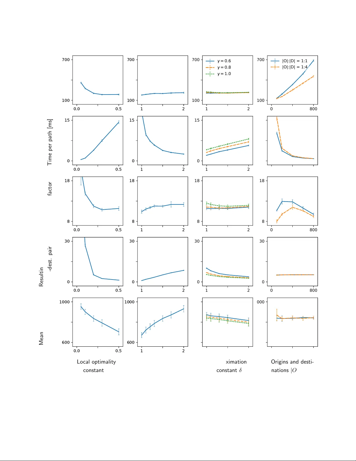
Lo cally Optimal Routes for Route Choice Sets Sam uel M. Fisc her ∗ Octob er 6, 2020 Abstract Route c hoice is often mo delled as a t w o-step pro cedure in whic h tra v ellers c ho ose their routes from small sets of promising candidates. Man y metho ds developed to iden tify such c hoice sets rely on assumptions ab out the mec hanisms b ehind the route c hoice and require corresp onding data sets. F urthermore, existing approaches often inv olv e considerable com- plexit y or pe rform man y repeated shortest path queries. This mak es it diﬃcult to apply these metho ds in comprehensiv e mo dels with n umerous origin-destination pairs. In this pap er, we address these issues b y developing an algorithm that eﬃcien tly iden tiﬁes lo cally optimal routes. Such paths arise from tra vellers acting rationally on local scales, whereas unknown factors ma y aﬀect the routes on larger scales. Though metho ds identifying lo cally optimal routes are a v ailable already , these algorithms rely on approximations and return only few, heuristically chosen paths for sp eciﬁc origin-destination pairs. This conﬂicts with the de- mands of route choice mo dels, where an exhaustive searc h for many origins and destinations w ould b e necessary . W e therefore extend existing algorithms to return (almost) all admissi- ble paths b etw een a large n umber of origin-destination pairs. W e test our algorithm and its applicabilit y in route c hoice mo dels on the road netw ork of the Canadian pro vince British Colum bia and empirical data collected in this pro vince. Keyw ords: alternativ e paths; c hoice set; computer algorithm; lo cal optimalit y; road netw ork; route choice. ∗ Departmen t of Mathematical and Statistical Sciences, Universit y of Alberta, Edmonton, AB T6G 2G1, Canada. Email: samuel.ﬁsc her@ualberta.ca 1 1 In tro duction Route choice mo dels hav e imp ortant applications in transp ortation netw ork planning ( Y ang & Bell , 1998 ), traﬃc control ( Mahmassani , 2001 ), and even epidemiology and ecology ( Fisc her et al. , 2020 ). Route c hoice mo dels can b e classiﬁed as either p erfect rationality mo dels or b ounded rationalit y mo dels ( Di & Liu , 2016 ). In p erfect rationalit y mo dels ( Sheﬃ , 1984 ), trav ellers are assumed to ha v e complete information and c hoose their routes optimally according to some go o dness criterion, whereas b ounded rationality mo dels ( Simon , 1957 ) take information constraints and the complexit y of the optimization pro cess into account. Though b oth p erfect rationalit y mo dels and b ounded rationalit y models ha ve b een used in route c hoice mo delling, b ounded rationalit y models ha v e b een found to ﬁt observed data b etter ( Di & Liu , 2016 ). Man y b ounded rationalit y models consider route c hoice as a tw o-stage pro cess: ﬁrst, a so- called “choice set” of p otentially go o d routes is generated, and second, a route from the choice set is c hosen according to some goo dness measure ( Ben-Akiv a et al. , 1984 ). This approac h is motiv ated through trav ellers’ limited abilit y to consider all p ossible paths. Instead, they may heuristically iden tify a small set of routes from whic h they choose the seemingly best. Besides this conceptual reasoning, the tw o-step mo del has computational adv an tages, as the c hoice sets can b e generated based on simple heuristics, while complex mo dels ma y b e applied to determine tra v ellers’ preferences for the identiﬁed routes. Therefore, the tw o-stage pro cess is widely used in route choice mo delling ( Prato , 2009 ). Most of the approaches to identify route choice sets are based on a com bination of the optimality assumption, the constraint assumption, and the sto chasticit y assumption. • According to the optimality assumption, tra vellers c ho ose routes optimally according to some criterion, which could b e based on route c haracteristics (e.g. tra v el costs and trav el time), or on scenarios (e.g. that the tra v el time on the shortest route increases). Examples include the link lab elling approach ( Ben-Akiv a et al. , 1984 ), link elimination ( Azevedo et al. , 1993 ), and link p enalty ( De La Barra et al. , 1993 ). • According to the constraint assumption, trav ellers consider all paths whose quality exceeds a 2 certain minimal v alue (e.g. acyclic paths not more than 25% longer than the shortest route). This assumption motiv ates constrained en umeration metho ds ( Prato & Bekhor , 2006 ). • The sto chasticit y assumption accoun ts for the p ossibilit y of sto chastic ﬂuctuations of route c haracteristics (e.g. through traﬃc jams or accidents) or error-prone information. Often, sto c hastic route c hoice sets are computed based on the optimality principle applied to a randomly p erturb ed graph (see Bovy , 2009 ). Though each of the assumptions men tioned ab o ve has a sound mechanistic justiﬁcation, they require that the heuristic that trav ellers use to identify p oten tially suitable paths is known and that corresp onding data are a v ailable. Ho w ev er, if tra v ellers c ho ose a route for unknown reasons, e.g. b ecause they desire to drive via some intermediate destination, their routes would b e diﬃcult to consider with the common metho ds. The natural solution w ould b e to increase the set of generated routes by relaxing constrain ts or mo delling more mechanisms explicitly . How ev er, in comprehensiv e and large-scale route choice mo dels, many origin-destination pairs may ha ve to b e considered, making it costly or even infeasible to work with large c hoice sets. Thus, it w ould b e desirable to characterize c hoice sets based on a more general but suﬃcien tly restrictive criterion that do es not require knowledge or data of the sp eciﬁc mec hanism b ehind route c hoices. A p otentially suitable criterion is lo c al optimality . A route is lo cally optimal if all its short (“lo cal”) subsections are optimal, respectively , according to a given measure. F or example, if trav el time is the applied go o dness criterion, a lo cally optimal route would not con tain lo cal detours. The rationale b ehind the principle of lo cal optimalit y is that the factors impacting trav ellers’ routing decisions ma y diﬀer dep enden t on the spatial scale. T ourists, for example, may w an t to driv e along the shortest route lo cally but plan their trip globally to include a num b er of sigh ts. Other trav ellers ma y w ant to driv e along the quic kest routes lo cally while minimizing the ov erall fuel consumption. Y et others may hav e a limited horizon of p erfect information and act rationally within this horizon only . Indep endent of the sp eciﬁc mechanism b ehind trav ellers’ route choices on the large scale, it is p ossible to characterize man y c hoice candidates as lo cally optimal routes. A p oten tial problem with considering lo cally optimal routes is that the set of lo cally optimal routes b et w een an origin and a destination can be very large and include zig-zag routes, whic h ma y 3 seem unnatural. A p ossible solution is to fo cus on so-called single-via p aths . A single-via path is the shortest path via a giv en in termediate lo cation. Since not all lo cally optimal paths are single-via paths, restricting the fo cus on single-via paths excludes some p otentially suitable paths from the choice set. Ho wev er, single-via paths hav e a reasonable mechanistic justiﬁcation through trav ellers choosing in termediate destinations, and the reduced c hoice sets are lik ely to include most of the routes that trav ellers would reasonably c ho ose. Since the reduced sets con tain relativ ely few elemen ts, sophisticated mo dels can b e used for the second decision stage, in which a route is chosen from the c hoice set. Therefore, constraining the searc h for lo cally optimal routes on single-via paths may lead to ov erall b etter ﬁtting route c hoice mo dels. T o date, methods iden tifying locally optimal single-via paths hav e been dev elop ed with the ob jective to suggest multiple routes to trav ellers ( Abraham et al. , 2013 ; Delling et al. , 2015 ; Luxen & Schieferdec ker , 2015 ; Bast et al. , 2016 ). Such suggestions of alternative routes are a common feature in routing softw are, suc h as Go ogle Maps or Bing Maps. Ho wev er, route choice mo dels ha v e diﬀeren t demands than routing soft w are, as trav ellers’ decisions shall b e mo del le d or pr e dicte d rather than facilitate d . Route planning soft w are seeks to compute a small n umber of high-quality paths that tra vellers ma y w ant to c ho ose. Here, computational sp eed is more imp ortan t than rigorous application of sp eciﬁc criteria c haracterizing the returned paths. In con trast, route c hoice mo dels should consider al l routes that trav ellers may take, and rigorous application of mo delling assumptions is k ey to allo w mechanistic inference and to mak e mo dels p ortable. In addition, route c hoice mo dels may consider multiple origins and destinations. Therefore, man y algorithms designed to facilitate route planning cannot b e directly applied to iden tify route choice sets. In this pap er, w e bridge this gap b y extending an algorithm originally designed for route planning. The algorithm REV by Abraham et al. ( 2013 ) searc hes a small num b er of “go o d” lo cally optimal paths b etw een a single origin-destination pair. T o this end, the algorithm uses an appro ximation causing some lo cally optimal paths to b e misclassiﬁed as sub optimal. Our extended algorithm o v ercomes these limitations. Unlik e REV, our algorithm returns (al- 4 most) al l admissible paths b et ween a set of origins and a set of destinations. Therefore, we call our algorithm REV C, the “C” emphasizing the attempted c omplete searc h. REV C identiﬁes lo- cally optimal routes with arbitrarily high precision. That is, the algorithm may falsely reject some lo cally optimal single-via routes, but the error can b e arbitrarily reduced b y cost of computational sp eed. As the execution time of REVC dep ends mostly on the num b er of distinct origins and destinations rather than the n umber of origin-destination p airs , the algorithm is an eﬀectiv e to ol to build traﬃc mo dels on comprehensiv e scales. This pap er is structured as follo ws: ﬁrst, we introduce helpful deﬁnitions and notation, review concepts we build on, and provide a clear deﬁnition of our ob jective. Then w e give an ov erview of REV C, b efore we decribe eac h step in detail. After describing the algorithm, we presen t results of numerical and empirical tests proving the algorithm’s applicabilit y and eﬃciency in real-w orld problems. Finally , we discuss the test results and the limitations and b eneﬁts of our approach. 2 Algorithm 2.1 Preliminaries In this section, w e sp ecify our goal and introduce helpful notation and concepts. First, we provide deﬁnitions and notation, which we then use to characterize the routes we are seeking. Afterwards, w e recapitulate Dijkstra’s algorithm and brieﬂy describ e the metho d of reac h based pruning, t w o basic concepts that our w ork builds on. 2.1.1 Problem statement and notation Supp ose w e are giv en a graph G = ( V , E ) that represents a road netw ork. The set of vertices V mo dels intersections of roads as w ell as the start and end p oin ts of in terest. The directed edges e ∈ E represent the roads of the road netw ork and are assigned non-negative weigh ts c e , denoting the costs for driving along the roads. T o ease notation, w e will refer to the cost of an edge or path as its length without loss of generality . In practice, other cost metrics, such as trav el time, may b e used. Our goal is to ﬁnd lo cally optimal paths b etw een all com binations of origin lo cations 5 s ∈ O ⊆ V and destination lo cations t ∈ D ⊆ V . T o sp ecify the desired paths more precisely , we introduce conv enient notation and make some deﬁnitions: P st is the shortest path from s to t . P uv is the subpath of P from u ∈ P to v ∈ P . l ( P ) is the length of the path P . That is, l ( P ) = P e ∈ P c e . d ( u, v ) := l ( P uv ) is the length of the shortest path from the v ertex u to the vertex v . d P ( u, v ) := l ( P uv ) is the length of the subpath of P from v ertex u to vertex v . With this notation, we in tro duce the notion of single-via p ath s. Deﬁnition 1. A single-via p ath (or short v-p ath ) P sv t via a vertex v is the shortest path from a v ertex s to a v ertex t via v . W e sa y v r epr esents the single-via path P sv t with resp ect to the origin-destination pair ( s, t ). F or simplicity , we assume that P st and P sv t are alw ays uniquely deﬁned. In practise, the paths are concatenations of shortest paths found by algorithms outlined b elo w, which are resp onsible for breaking ties. W e pro ceed with a precise deﬁnition of lo cal optimality following Abraham et al. ( 2013 ). Gen- erally speaking, a path is T -locally optimal if eac h subpath of P with a length of at most T is a shortest path. Ho w ever, b ecause paths are concatenations of discrete elements, w e need a more tec hnical deﬁnition. Deﬁnition 2. Consider a subpath P 0 ⊆ P and let P 00 ⊂ P 0 b e P 0 after remov al of its end p oints. W e sa y P 0 is a T -signiﬁc ant subpath of P if l ( P 00 ) < T . A path P is T - lo c al ly optimal if all its T -signiﬁcan t subpaths P 0 are shortest paths. W e say P is α -r elative lo c al ly optimal if it is T -lo cally optimal with T = α · l ( P ). W e w an t to iden tify locally optimal paths b etw een man y origin and destination locations. Ho w ever, there ma y b e an excessive n umber of such paths. Therefore, w e apply slightly stronger constrain ts on the searched paths, whic h w e will call admissible b elow. 6 Deﬁnition 3. Let α ∈ (0 , 1] and β ≥ 1 b e constants. A v-path P sv t from vertex s ∈ O to v ertex t ∈ D via vertex v ∈ V is called admissible if 1. P sv t is α -relativ e lo cally optimal. 2. P sv t is longer than the shortest path by no more than factor β , i.e. l ( P sv t ) ≤ β · l ( P st ). Ob jective. The ob jectiv e of this pap er is to iden tify (close to) all admissible single-via paths b et ween eac h origin s ∈ O and each destination t ∈ D . 2.1.2 Dijkstra’s algorithm Large parts of our algorithm are based on mo diﬁcations of Dijkstra’s algorithm ( Dijkstra , 1959 ; Dan tzig , 1998 ). Dijkstra’s algorithm is a frequently used metho d to ﬁnd the shortest paths from an origin s to all other v ertices in a graph with non-negative edge w eights. Though the algorithm is well-kno wn to a large audience, we brieﬂy recapitulate the algorithm to establish some notation that we will use later. • In Dijkstra’s algorithm, ev ery v ertex v is assigned a speciﬁc cost denoted cost( v ). Even tually , this cost shall b e equal to the distance b etw een the origin vertex s and v ertex v . Initially , ho w ever, the cost of each vertex is ∞ . An exception is the origin s , for which the initial cost is 0. • W e sa y that a vertex v is sc anne d if we are certain that cost( v ) = d ( s, v ). F urthermore, we sa y that a not yet scanned v ertex v is lab el le d if cost( v ) < ∞ . All other v ertices are called unr e ache d . In line with our notion of scanned vertices, we call edges e = ( u, v ) scanned if we kno w that e ∈ P sv for some scanned vertex v . Dijkstra’s algorithm is outlined in Algorithm 1 . Initially , all v ertices are in a container that allo ws us to determine the least-cost vertex eﬃciently . Dijkstra’s algorithm consecutively remov es the least-cost v ertex v from the container and scans it. That is, the algorithm iterates o ver v ’s successors w and up dates their costs if the distance from the origin s to w via v is smaller than the current cost of w . In this case, v is sav ed as the p ar ent of w . 7 Algorithm 1: Dijkstra’s algorithm. 1 while c ontainer is not empty do 2 T ake the v ertex with the low est cost from the container and remov e it; 3 Sc an the vertex v : 4 forall suc c essors of v that have not b e en sc anne d yet do 5 L ab el w : 6 if cost( w ) < cost( v ) + c v w then 7 Set cost( w ) := cost( v ) + c v w ; // c v w is the length of the edge from v to w 8 Set parent ( w ) := v ; After execution of Dijkstra’s algorithm, shortest paths can b e reconstructed b y following the trace of the computed paren t vertices, starting at the destination v ertex and ending at the origin. The edges (paren t ( v ) , v ) for all scanned v ertices v ∈ V form a shortest p ath tr e e . Hence, we call the pro cedure describ ed ab ov e “growing a shortest path tree”. The distance (measured in cost units) from the start v ertex to its farthest descendant is called the height of the shortest path tree. As w e will see b elow, it can b e b eneﬁcial to stop the tree growth when the tree has reached a certain heigh t. When the shortest path b etw een a sp eciﬁc pair of v ertices s and t is sough t, the bidir e ctional Dijkstr a algorithm is more eﬃcient than the classic algorithm (compare Figures 1 (a) and (b)). The bidirectional Dijkstra algorithm grows t wo shortest path trees: one in forward direction starting at the origin s and one in backw ard direction starting at the destination t . The trees are grown sim ultaneously; i.e., the resp ective tree with smaller height is grown un til its height exceeds the other tree’s height. The search terminates if a vertex v is included in b oth trees, i.e., scanned from b oth directions. The shortest path is the concatenation of the s - v path in the ﬁrst shortest path tree and the v - t path in the second tree. 8 s t a ) b ) c) s t s t v v 2 v 1 v 3 Figure 1: Conceptual illustration of diﬀerent path search algorithms for an origin s and a destination t . The shaded areas depict shortest path trees. (a) Dijkstra’s algorithm grows a single shortest path tree around the origin un til the destination is reached. (b) The bidirectional Dijkstra algorithm gro ws a forward tree around the origin and a bac kward tree around the destination until the tw o shortest path trees meet at a vertex v . (c) Multiple v-paths can b e constructed b y growing ov erlapping shortest path trees around origin and destination. Figures (a) and (b) are redra wn from Bast et al. ( 2016 ). 2.1.3 Reac h-based pruning Dijkstra’s algorithm is not eﬃcient enough to ﬁnd shortest paths in large netw orks within reason- able time. Therefore, m ultiple metho ds ha ve b een developed to iden tify and prune vertices that cannot b e on the shortest path. One of these approac hes is reac h-based pruning (RE; Goldb erg et al. , 2006 ), which w e in tro duce b elow. Let us start by in tro ducing the notion of a vertex’s reac h. Deﬁnition 4. The r e ach of a v ertex v is deﬁned as reac h( v ) := max u,w ∈ V : v ∈ P uw { min ( d ( u, v ) , d ( v , w )) } . (1) That is, if we consider all shortest paths that include v , split each of these paths at v , and consider the shorter of the t wo ends, then the reach of v is the maximal length of these sections. The reach of v is high if v is at the cen tre of a long shortest path. T ypically , vertices on high w ays ha ve a high reach, since man y long shortest paths include highw ays. Disregarding vertices with small reac hes can sp eed up shortest path searches. Supp ose we use the bidirectional Dijkstra algorithm to ﬁnd the shortest path b etw een the vertices s and t and ha v e already grown shortest path trees with heights h . Let v ∈ P st b e a vertex that is lo cated on the shortest path b et ween s and t but has not b een scanned y et. Then d ( s, v ) > h and d ( v , t ) > h , since v would hav e b een included in one of the shortest path trees otherwise. Therefore, w e know 9 s t a ) b) c) s t s t v v 1 v 2 d ) s 1 s 2 t v Figure 2: Optimizations that REVC employs to eﬃciently iden tify admissible v-paths b etw een origin-destination pairs ( s, t ). (a) Shortest path trees (depicted as shaded areas) are grown to a tight b ound only and exclude low- reac h vertices, which cannot b e on long locally optimal paths. (b) U-turn paths (e.g. s → v → t ) are excluded b y requiring that an edge adjacent to the via v ertex is included b oth in the shortest path tree around the origin (blac k arrows) and the shortest path tree around the destination (blue arrows). Edges satisfying this constraint are highligh ted with red background. Note that arrows with diﬀerent directions depict distinct edges. (c) If v-paths via diﬀeren t v ertices v 1 and v 2 are identical, only one of these vertices is c hosen to represent the path. (d) If v-paths for diﬀerent origin-destination pairs (here: ( s 1 , t ) and ( s 2 , t )) are represented by the same via vertex v and share a subpath (highligh ted red), the lo cal optimality of this section is tested only once for all origin-destination pairs. that reach( v ) ≥ min ( d ( s, v ) , d ( v , t )) > h . Thus, when adding further vertices to our shortest path trees, we can neglect all v ertices with a reach less or equal to h . This sp eeds up the shortest path searc h. Computing the precise reac hes of all vertices is exp ensiv e, as this w ould require an extremely large n um b er of shortest path queries. How ever, Goldb erg et al. ( 2006 ) dev elop ed an algorithm to compute upp er b ounds on vertices’ reac hes eﬃciently . These upp er b ounds can b e used in the same wa y as exact v ertex reac hes. 2.2 Outline of the algorithm After sp ecifying our goal and in tro ducing necessary notation and concepts, w e can no w pro ceed with an o verview of our algorithm. The main idea of REVC is (1) to grow shortest path trees in forward direction from all origins and in backw ard direction from all destinations and (2) to c hec k the admissibilit y of the v-paths via the vertices that ha ve b een scanned in b oth forw ard and bac kw ard direction (see Figure 1 c). F or eac h v ertex v that is scanned b oth from an origin s and a destination t , the v-path P sv t can b e reconstructed easily from the information contained in the shortest path trees. Therefore, the only remaining step is to chec k whether P sv t is admissible, i.e. lo cally optimal and not muc h longer than the shortest path P st . 10 G r o w f o r w a r d sh o r t e st p a t h s a r o u n d o r i g i n s G r o w b a ckw a r d sh o r t e st p a t h s a r o u n d d e st i n a t i o n s S e l e ct e d g e s sca n n e d i n b o t h d i r e ct i o n s E l i m i n a t e e d g e s s ca n n e d f r o m t h e sa m e o r i g i n s a n d d e st i n a t i o n s a s t h e i r n e i g h b o u r s C o n si d e r v- p a t h s v i a e n d p o i n t s o f t h e r e m a i n i n g e d g e s. E l i m i n a t e e q u a l p a t h s E l i m i n a t e o ve r l y l o n g p a t h s E l i m i n a t e l o ca l l y su b o p t i m a l p a t h s S t e p 1 S t e p 2 S t e p 3 S t e p 4 Figure 3: Ov erview of REV C. As each v ertex v ∈ V could serv e as via v ertex for many origin-destination com binations, c hec king the admissibility of all possible v-paths ma y b e infeasible. Therefore, it is imp ortan t to iden tify and exclude v ertices that cannot represent admissible v-paths. The follo wing observ ations can b e exploited: (1) v-paths via vertices that are v ery far from an origin or destination cannot fulﬁll the length requiremen t. (2) Some v ertices represen t intersections of minor roads, which can b e b ypassed on close-b y ma jor roads. Thus, these v ertices cannot b e part of lo cally optimal paths. (3) Some v-paths may include a u-turn at the via vertex (see Figure 2 b). That is, tra vellers driving on such a path would need to drive bac k and forth along the same road. This is not lo cally optimal b ehaviour. (4) Some via v ertices may represen t the same v-paths. That is, the v-paths corresp onding to distinct via v ertices ma y b e identical, and only one of these via vertices needs to b e considered. Our algorithm REVC mak es use of the observ ations listed ab o ve. (1) When shortest path trees are grown around eac h origin and destination, the trees are grown up to a tightly sp eciﬁed height only . That w a y , many v ertices that are to o far oﬀ will not b e scanned. (2) When the shortest path trees are grown, reach based pruning is applied to exclude vertices that are not on any suﬃciently lo cally optimal path (see Figure 2 a). (3) Instead of considering all v-paths via v ertices scanned in forw ard and bac kward direction, REV C considers only v-paths in whic h an e dge adjacen t to the via v ertex has b een scanned forward and bac kward. This excludes paths inv olving u-turns (see 11 Figure 2 b). (4) Before chec king the admissibility of the remaining v-paths, the algorithm ensures that each v-path is represen ted b y one vertex only (see Figure 2 c). After these steps, REVC excludes v-paths that are exceedingly long and chec ks whic h v-paths are suﬃciently lo cally optimal. T esting whether all v-paths P sv t via a sp eciﬁc vertex v are lo cally optimal would b e exp ensive if eac h origin-destination pair ( s, t ) ∈ O × D w ere considered indi- vidually . Therefore, REVC chec ks the admissibility of man y paths simultaneously , reusing earlier results and applying approximations. That wa y , the algorithm b ecomes muc h more eﬃcient than individual pair-wise searc hes for admissible paths (see Figure 2 d). In Figure 3 , we provide an o v erview of REV C. Before the actual algorithm can b e started, some preparational work and prepro cessing is required. W e will provide a detailed description of the prepro cessing procedure after in tro ducing the algorithm in detail. 2.3 Step 1: Growing shortest path trees The algorithm REVC starts b y growing forward shortest path trees out of each origin and backw ard shortest path trees in to each destination. F or each admissible v-path P , w e need to scan at least one v ertex v with P = P sv t from b oth the origin s and the destination t . In addition, we wan t to scan one edge e ∈ P adjacen t to v from b oth directions if p ossible. These edges will b e used to exclude u-turn paths. F or eac h v ertex v included in a shortest path tree, w e note v ’s predecessor and heigh t in the tree. F urthermore, w e memorize from whic h origins and destinations eac h edge has b een scanned. 2.3.1 T ree b ound T o sa ve the work of scanning vertices inadmissibly far a wa y from the origins and destinations, we aim to stop the tree growth as so on as p ossible. W e need to scan at least one v ertex v for each admissible path P sv t with a length l ( P sv t ) = d ( s, v ) + d ( v , t ) ≤ β · l ( P st ). Since either of d ( s, v ) and d ( v , t ) could b e arbitrarily small, the algorithm REV b y Abraham et al. ( 2013 ) grows the trees up to a height of β · l ( P st ). Nev ertheless, w e can terminate the search earlier if w e take in to account 12 that we are searc hing for lo cally optimal paths. T o deriv e a tighter tree b ound, note that for an α -relative lo cally optimal path P , each sub- section with length α · l ( P ) is a shortest path. This is in particular true for the subsection P 0 ⊆ P starting at the origin. Since P 0 is a shortest path, the end p oint x s of this subsection will be included in the origin’s shortest path tree. Therefore, it suﬃces to grow the destination’s shortest path tree until x s is reached, which is closer to t than β · l ( P st ). The same applies in the rev erse direction. T o sp ecify the tree b ound, deﬁne x s ∈ P more precisely to b e the ﬁrst v ertex that is farther a w ay from the origin than α · l ( P ). If this v ertex is lo cated in the second half of the path, c hange x s to b e the last v ertex in the ﬁrst half of P . Cho ose x t accordingly in relation to the destination. Our observ ations from ab ov e are formalized in the following lemma and corollary , whic h we prov e in App endix A . Lemma 1. With s , t , x s , x t , and P deﬁne d as ab ove, ther e is at le ast one vertex v ∈ P with 1. d P ( s, v ) = d ( s, v ) ≤ d P ( s, x t ) and 2. d P ( v , t ) = d ( v , t ) ≤ d P ( x s , t ) . Corollary 1. F or e ach admissible v-p ath b etwe en an origin-destination p air ( s, t ) , a via vertex wil l b e sc anne d fr om b oth dir e ctions if the shortest p ath tr e es ar e gr own up to a height of h max := max  (1 − α ) β l ( P st ) , 1 2 β l ( P st )  . (2) In Corollary 1 , w e consider a single origin-destination pair. Ho wev er, w e w ant to identify admissible paths b et w een m ultiple origins and destinations and ha v e to adjust the tree b ound accordingly . The tree around eac h origin and destination shall b e large enough to include via v ertices for al l paths starting at the resp ective endp oint. Hence, if we gro w a tree out of origin s , w e grow it to a heigh t of max  (1 − α ) β M s , 1 2 β M s  with M s = max t ∈ D l ( P st ). W e pro ceed with destinations similarly . Note that the tree b ounds ab o v e can only b e determined if the shortest distances b etw een the origins and destinations are kno wn. Though these distances can b e determined while the shortest 13 path trees are grown, we will see in the next section that the shortest distances can also b e used to sp eed up the tree growth itself. Therefore, it is b eneﬁcial to determine the shortest distances in a prepro cessing stage. This also makes it easy to grow the trees in parallel. 2.3.2 Pruning the trees The search for admissible paths can b e signiﬁcan tly sp ed up if vertices with small reach v alues are ignored when the shortest paths are grown. Consider a vertex v on an admissible s - t path P . Let us regard the subpath P 0 that is centred at v and has a length just greater than α · l ( P ). Since P is α -relativ e lo cally optimal, w e know that P 0 is a shortest path. F urthermore, P 0 is roughly split in half by v , unless v is close to one of the end p oin ts of P . Th us, reac h( v ) ≥ min n α 2 l ( P ) , d ( s, v ) , d ( v , t ) o (3) (see Lemma 5.1 in Abraham et al. , 2013 ). If we are growing the tree out of origin s , w e can use ( 3 ) to prune the successors of v ertices v with reac h( v ) < min  α 2 l ( P ) , d ( s, v )  . Pruning the successors but not v itself ensures that at least one vertex p er admissible path is scanned from b oth directions, ev en if ( 3 ) is dominated by d ( v , t ). Since l ( P ) is unkno wn when the shortest path trees are grown, the length of P must b e b ounded with known quantities. Abraham et al. ( 2013 ) use the triangle inequality l ( P ) ≥ d ( s, v ) + d ( v , t ) ≥ cost( v ) . (4) Ho w ever, w e can also determine shortest distances b efore we search admissible paths and ex- ploit that P ≥ d ( s, t ) or, if we are considering multiple origins and destinations, l ( P ) ≥ L s := min ˜ t ∈ D d  s, ˜ t  . Therefore, w e ma y prune the successors of vertices v with reac h( v ) < min n cost( v ) , α 2 max { cost( v ) , L s } o (5) when we grow the shortest path tree out of origin s . 14 W e can prune even more vertices if w e grow the trees in forward and bac kw ard direction in separate steps. The idea is to use data collected in the ﬁrst step to derive a sharp er pruning b ound for the second step. Whether w e grow the forward or the bac kward trees in the ﬁrst step dep ends on whether there are more destinations or more origins to pro cess. Below w e assume without loss of generality that w e consider more destinations than origins, | D | ≥ | O | . W e pro ceed as follows: w e start b y growing the forward trees out of the origins. In this phase, w e prune v ertices’ successors according to inequality ( 5 ). After gro wing the forw ard trees, w e determine for each scanned v ertex v the distance d min ( v ) := min s ∈ O ; v scanned from s d ( s, v ) to the closest origin it has b een scanned from. If v has not b een scanned, w e set d min ( v ) := ∞ . No w w e gro w the bac kw ard trees and use d min ( v ) as a lo wer b ound for d ( s, v ) for all origins s ∈ O . Hence, w e can prune all vertices with reac h( v ) < min n cost( v ) , α 2 max { cost( v ) , L t } , d min ( v ) o . (6) In con trast to criterion ( 5 ), we can apply criterion ( 6 ) directly to eac h v ertex v and not only to its successors. This decreases the n umber of considered v ertices. W e provide pseudo code for the tree growth pro cedures in Algorithms 2 and 3 . 2.3.3 Determining p oten tial via v ertices With the shortest path trees, w e can determine whic h v ertices ma y potentially represent admissible v-paths. Each v ertex scanned in forw ard and bac kw ard direction could be suc h a via v ertex. Ho w ever, since some of the resulting paths could include u-turns, w e consider the scanned e dges rather than the vertices. This excludes paths with u-turns (see Figure 4 ). W e pro ceed as follo ws: w e determine for each scanned edge e the sets O e and D e of origins and destinations that e has b een scanned from. W e discard all edges that hav e not b een scanned from at least one origin and one destination. Let E via b e the resulting set of edges. The set of considered via vertices V via := { v ∈ V | ∃ w ∈ V : ( v , w ) ∈ E via } is given b y the starting p oints of the edges in E via . Note that though the pro cedure ab ov e eliminates paths with u-turns, some admissible v-paths 15 Algorithm 2: Growing a forward shortest path tree out of origin s . 1 while c ontainer is not empty do 2 T ake the v ertex v with the low est cost from the container and remov e it; 3 Mark edge leading to v as visited from origin s ; 4 Include v in the shortest path tree; 5 if d min ( v ) > cost( v ) then 6 d min ( v ) := cost( v ); 7 if reach( v ) ≥ min  cost ( v ) , α 2 max (cost( v ) , L s )  then 8 Scan the vertex v ; // see Algorithm 1 Algorithm 3: Growing a forward shortest path into destination t . 1 while c ontainer is not empty do 2 T ake the v ertex v with the low est cost from the container and remov e it; 3 Mark edge leading to v as visited from destination t ; 4 if reach( v ) ≥ min  cost( v ) , α 2 max (cost( v ) , L t )  then 5 Include v in the shortest path tree; 6 Sc an the vertex v with e arly pruning: 7 forall neighb ors w of v that have not b e en sc anne d yet do 8 new C ost := cost( v ) + d ( v , w ); 9 if reach( v ) ≥ min  new C ost, α 2 max ( new C ost, L t ) , d min ( v )  then 10 Lab el w ; // see Algorithm 1 s t Figure 4: Adv an tages of considering via edges instead of via v ertices. Arrows highlighted in dark blue depict the forw ard shortest path tree grown from the origin s , and arro ws highlighted in light red represen t the backw ard tree gro wn into the destination t . Edges that are scanned from b oth directions are p otential via edges and drawn as solid blac k lines. The remaining edges are drawn as dashed blac k lines. All v ertices are scanned both from s and t and would therefore considered p otential via v ertices. Ho wev er, paths via the tw o topmost vertices w ould require a u-turn. Restricting the fo cus on v-paths via vertices adjacent to the solid lines excludes these u-turn paths. 16 ma y b e rejected as well. How ever, this issue will rarely o ccur in realistic road netw orks, since the problem arises only at sp eciﬁc merging p oints of v ery long edges. W e provide details in App endix B . 2.4 Step 2: Identifying vertices representing identical v-paths Some of the vertices in V via ma y represent iden tical v-paths. Since we wan t to sa ve the eﬀort of c hec king the admissibility of the same path m ultiple times and, similarly imp ortan tly , w e do not w an t to return multiple iden tical paths, we need to ensure that eac h admissible path is represented b y one via vertex only . T o identify v ertices represen ting iden tical paths, we ha ve to compare the v-paths corresp onding to all v ∈ V via for each origin-destination pair. This requires O ( | V via | | O | | D | ) steps. Ho wev er, for some vertices, identical paths can b e iden tiﬁed more quic kly , as adjacent v ertices typically represent similar sets of v-paths. Therefore, we pro ceed in tw o steps: ﬁrst, we reduce V via b y eliminating v ertices whose via paths are also represen ted by their resp ective neighbours, and second, w e c hec k whic h of the remaining v ertices represen t iden tical v-paths. Below we describ e the t w o steps in greater detail. 2.4.1 Eliminating vertices that represen t the same v-paths as their neighbours The endpoints of an edge can b e neglected as via vertices if the edge has b een scanned from the same origins and destinations as a neigh b ouring edge. Consider for example an edge ( v , w ) that has b een scanned from b oth an origin s and a destination t . Then P sw = P sv w and P v t = P v wt . It follo ws that v and w represen t the same v-path with resp ect to ( s, t ): P sv t = P swt . Now consider an adjacent edge ( u, v ) that has b een scanned from s and t as w ell. Clearly , it is P sut = P sv t and P sv t = P swt , whic h implies that the v-paths via u , v , and w are iden tical. Therefore, only one of these vertices has to b e considered. T o introduce an algorithm that eﬃciently detects suc h conﬁgurations, let O e b e the set of origins and D e the set of destinations that edge e has b een scanned from. F or eac h edge e ∈ E via , w e chec k whether one directly preceding edge e 0 ∈ E via has b een scanned from a sup erset of origins 17 and destinations, i.e. O e ⊆ O e 0 and D e ⊆ D e 0 . If such an edge exists and one of the set inequalities holds strictly , i.e. O e ⊂ O e 0 or D e ⊂ D e 0 , w e may disregard edge e , as all v-paths via e are also v-paths via e 0 . Things b ecome more complicated if O e = O e 0 and D e = D e 0 , as we may either reject e , e 0 , or b oth edges. The latter case ma y o ccur if e 0 has another directly preceding edge e 00 ∈ E via with O e 0 ⊆ O e 00 and D e 0 ⊆ D e 00 . If one of these inequalities is strict, we disregard both e and e 0 . Otherwise, w e contin ue trav ersing the edges in E via un til either (1) an edge is found whose origin and destination sets sup ersede the sets of all previous edges or (2) no further predecessor with suﬃcien tly large origin and destination sets is found. In the second case, we may disregard all trav ersed edges but e . W e apply the same approac h to the successors of e and rep eat this pro cedure un til all edges in E via ha v e b een pro cessed. The up dated set V via of via vertices consists of the starting v ertices of the edges in the reduced edge set E via . W e pro vide pseudo co de for the outlined algorithm in Algorithm 4 . An eﬃcient implemen tation ma y compa re the origin and destination sets of the edges in E via b efore the trav erse is started. This mak es it easy to implement the most exp ensive parts of the algorithm in parallel. 2.4.2 Iden tifying remaining iden tical v-paths The metho d outlined ab o v e identiﬁes v ertices that represent the same v-paths as their neighbours. Ho w ever, tw o vertices may represen t the same v-path with resp ect to one origin-destination pair but diﬀerent v-paths with resp ect to another origin-destination pair. Consequen tly , these v ertices could not b e rejected in the step describ ed ab ov e, and a second pro cedure is required to eliminate the remaining identical v-paths. W e iden tify the remaining identical v-paths b y comparing path lengths. T o this end, w e assume that P sv t = P swt if and only if l ( P sv t ) = l ( P swt ). Though it can happ en that distinct paths ha v e the same length, this case is usually not of greater concern in practical applications. The issue can b e reduced by introducing a small random p erturbation for the lengths of edges. W e examine this limitation further in the discussion section. With the ab o ve assumption, iden tical paths can b e identiﬁed eﬃcien tly . Since for each origin- 18 Algorithm 4: Eliminating vertices that represent the same v-paths as their neighbours. 1 F unction has superior predecessor( e ) : 2 Remo v e e from E via ; 3 forall dir e ctly pr e c e ding e dges e 0 of e do 4 if O e ⊆ O e 0 and D e ⊆ D e 0 then 5 if O e = O e 0 and D e = D e 0 then 6 return has superior predecessor( e 0 ) 7 else 8 return T rue; 9 return F alse; 10 F unction has superior successor( e ) : 11 Remo v e e from E via ; 12 forall dir e ctly suc c e e ding e dges e 0 of e do 13 if O e ⊆ O e 0 and D e ⊆ D e 0 then 14 if O e = O e 0 and D e = D e 0 then 15 return has superior successor( e 0 ) 16 else 17 return T rue; 18 return F alse; 19 E 0 via := ∅ ; 20 while E via 6 = ∅ do 21 Set e := next en try in E 0 via ; 22 if not has superior predecessor( e ) and not has superior successor( e ) then 23 Add e to E 0 via ; 24 E via := E 0 via ; 19 destination pair ( s, t ) and each potential via vertex v ∈ V via the distances d ( s, v ) and d ( v , t ) are kno wn, the v-path lengths can b e computed easily . F or eac h origin-destination pair, a comparison of the lengths of the v-paths corresp onding to all v ∈ V via can b e conducted in linear av erage time via hash maps. Note that the path lengths m ust b e compared with an appropriate tolerance for mac hine imprecision. In later steps it will b e of b eneﬁt if most v-paths are represen ted b y a small set of via v ertices. If there are multiple v ertices represen ting the same v-paths, w e therefore choose the via vertex v that has b een scanned from the most origin-destination combinations O v × D v . This mak es it easier to reuse partial results when we chec k whether the v-paths are lo cally optimal. 2.5 Step 3: Excluding long paths Before w e chec k whether paths are suﬃciently lo cally optimal, we exclude the paths that exceed the length allow ance. That is, w e disregard all paths P sv t with l ( P sv t ) > β · l ( P st ) with origin- destination pairs ( s, t ) and via vertices v ∈ V via . Since this step in v olves a simple comparison only , it is computationally c heap er than identifying identical paths. Therefore, it is eﬃcien t to conduct this step just b efore identical paths are eliminated (section 2.4.2 ). This also reduces the memory required to store p otentially admissible com binations ( s, v , t ) of origin-destination pairs and via v ertices. 2.6 Step 4: Excluding lo cally sub optimal paths The most challenging part of the searc h for admissible paths is to chec k whether paths are suf- ﬁcien tly locally optimal. T o test whether a subpath is optimal, we need to ﬁnd the shortest alternativ e, whic h is computationally costly . Therefore, we apply an appro ximation to limit the n um b er of necessary shortest path queries. Our metho d generalizes the approximate lo cal optimalit y test by Abraham et al. ( 2013 ). They noted that v-paths are concatenations of t wo optimal paths. Hence, v-paths are lo cally optimal ev erywhere except in a neigh b ourho o d of the via v ertex. More precisely , a v-path P sv t from s to t via v is guaranteed to b e T -lo cally optimal ev erywhere except in the section that b egins T 20 distance units b efore v and ends T distance units after v . Therefore, Abraham et al. ( 2013 ) suggest to p erform a shortest path query b etw een the end p oints x and y of this section to chec k whether it is optimal. Abraham et al. ( 2013 ) call this pro cedure the T-test. The T-test do es not return false p ositives. That is, a path that is not T -locally optimal will nev er b e misclassiﬁed as lo cally optimal. How ever, the T-test ma y return false negatives: paths that are T -lo cally optimal but not 2 T -lo cally optimal may b e rejected. In mo delling applications, a more precise lo cal optimality test may b e desired. It is p ossible to increase the precision of the T-test. Instead of c hecking whether the whole p oten tially suboptimal subpath is optimal, w e may test multiple subsections to gain a higher accuracy . While this pro cedure ensures that few er admissible paths are falsely rejected, the gain in accuracy comes with an increase in computational cost. Therefore, it is desirable to use the results of earlier lo cal optimality c hec ks to test the admissibility of other paths. There are tw o situations in whic h lo cal optimalit y results can b e reused. First, if a subsection of a path is found to b e sub optimal, other paths that include this section can b e rejected as well. Second, if a subpath of a path is found to be lo cally optimal, other paths including this subpath ma y b e classiﬁed as lo cally optimal as well. That wa y , many paths can b e pro cessed all at once. When reusing partial results, it is imp ortan t to note that ev en though w e require all paths to b e α -relative lo cally optimal, the absolute lengths of the subsections that need to b e optimal dep end on how long the considered paths are. Therefore, paths must b e considered in an order dep enden t on their lengths. W e provide details b elow. 2.6.1 Preparation Before we can start testing whether the remaining v-paths are lo cally optimal, a preparation step is needed to identify the subpaths that may b e suboptimal and thus need to b e assessed more closely . T o reuse partial results eﬃciently , we furthermore need to determine subsections that diﬀeren t paths hav e in common. W e describ e the preparation pro cedure b elo w. W e start b y introducing helpful notation. Supp ose w e wan t to test whether the v-paths via v ertex v are lo cally optimal. Let ˜ O := { s ∈ O | ∃ t ∈ D : l ( P sv t ) ≤ β · l ( P st ) } b e the origins for 21 whic h at least one destination can b e reached via v without violating the length constraint. Let ˜ D b e deﬁned accordingly for the destinations. Deﬁne ˜ D s := n t ∈ ˜ D | l ( P sv t ) ≤ β · l ( P st ) o as the set of destinations that can b e reached from the origin s via v without violating the length constraint. In the preparation step, w e determine for eac h origin s ∈ ˜ O the destination t s := argmax t ∈ ˜ D s l ( P sv t ) for which the potentially sub optimal section is longest. F urthermore, we searc h for the vertex x s := argmin ˜ x ∈ P sv ; d ( ˜ x,v ) ≥ αl ( P svt s ) d ( ˜ x, v ), which is the last vertex on P sv with d ( x s , v ) ≥ α · l ( P sv t s ), and we determine x t deﬁned accordingly . No w we ﬁll the arra ys A us :=        T rue if u ∈ P sv F alse else, A ut :=        T rue if u ∈ P v t F alse else (7) for all vertices u ∈ P x s v and u ∈ P v x t , resp ectiv ely . The information sa ved in the shortest path trees are suitable to ﬁnd paths from scanned vertices to the origins and destinations. How ever, the trees con tain no information on the reverse paths starting at the end points. That is, while it is easy to ﬁnd the bac kward shortest path from v to x s , it is hard to follo w the path in the opp osite direction starting at x s . W e gather the necessary information in the preparation step: for each origin s ∈ ˜ O , we sav e the successors of each relev ant v ertex u ∈ P sv . In Algorithm 5 , we pro vide pseudo co de for the describ ed pro cedures. The pseudo-co de con- siders the origins only . The algorithm for the destinations is similar. The preparation phase ends with sorting all origin-destination pairs with resp ect to the lengths of the resp ectiv e v-paths via v . 2.6.2 T esting lo cal optimality for one origin-destination pair W e use an appro ximation approac h with ﬂexible precision to c heck whether paths are locally optimal. F or a parameter δ ∈ [1 , 2], we call this pro cedure the T δ -test. The parameter δ is a measure for the test’s precision. T o outline the T δ -test, let us consider a v-path P := P sv t from s to t via the v ertex v . Let S s := { u ∈ P sv | d ( u, v ) < T } be the set of v ertices that are on the path P sv and ha ve a distance less 22 Algorithm 5: Filling the array A for the origins and ﬁnding successors. The algorithm for the destinations is similar. 1 foreac h destination s ∈ ˜ O do 2 t s := argmax t ∈ ˜ D s ( d ( s, v ) + d ( v , t )); 3 u := paren t s ( v ); 4 successor s ( u ) := v ; 5 stop := F alse; 6 while not stop do 7 if u / ∈ A then 8 Initialize A u ˜ s := F alse for all ˜ s ∈ ˜ O ; 9 A us := T rue; 10 successor s (paren t ( u )) := u ; 11 if d ( v , u ) > α ( d ( s, v ) + d ( v , t s )) then 12 stop := T rue; 13 else 14 u := paren t ( u ); than T to the vertex v . F urthermore, add to S s the vertex x := argmin ˜ x ∈ P sv ; d ( ˜ x,v ) ≥ T d ( ˜ x, v ) that is closest to v but has d ( x, v ) ≥ T if such a v ertex exists. Cho ose S t accordingly with resp ect to the destination v ertex t . Let partner t ( u ; τ ) := argmin ˜ w ∈ S t ; d P ( u, ˜ w ) ≥ τ d P ( u, ˜ w ) for u ∈ S s b e the v ertex w ∈ S t that is closest to u but has d P ( u, w ) ≥ τ . If no suc h v ertex exists in S t , set partner t ( u ; τ ) = y := argmax ˜ w ∈ S t d P ( u, ˜ w ). Deﬁne accordingly partner s ( w ; τ ) for w ∈ S t as the vertex u ∈ S s that is closest to w but has d P ( u, w ) ≥ τ . The T δ -test pro ceeds as follows: the algorithm starts at the v ertex u 1 := x and c hecks whether the subpath P u 1 w 1 b et ween u 1 and w 1 := partner t ( u 1 ; δ T ) is a shortest path. If so, the algorithm progresses searching u 2 := partner s ( u 1 ; T ) in backw ard direction and rep eats the steps formerly applied to u 1 no w with u 2 . This pro cedure rep eats un til u n = v for some n ∈ N . If all the shortest path queries yield subpaths of P , the path is deemed approximately T -lo cally optimal. Otherwise, it is classiﬁed as not lo cally optimal. W e depict the algorithm in Figure 5 and provide pseudo-code in Algorithm 6 . 23 u 1 w 1 := p artne r t ( u 1 ; δT ) s t x δ T v partne r s (w 1 ; T ) = : u 2 w 1 s t x T v u 2 w 2 : = par t ne r t (u 2 ; δ T ) s t x δ T v y y y a) b ) c) Figure 5: T δ -test with δ = 1 . 4. The three subﬁgures depict the steps of the T δ -test for a path P sv t connecting origin- destination pair ( s, t ) via vertex v . The vertices x and y are the end p oints of the p otentially lo cally sub optimal section. The edge lengths are giv en b y the Euclidean distance except for the edges with an indicated gap. (a) In a ﬁrst step, the test determines the vertex w 1 that is at least δ T units along the path aw ay from u 1 := x (the distance is depicted as blue arrow). (b) If the shortest path query betw een u 1 and w 1 indicates that the subsection P u 1 w 1 sv t is optimal, the test contin ues by determining the ﬁrst v ertex u 2 that is at least T units aw ay from w 1 in backw ards direction. (c) F rom u 2 , the algorithm searches the vertex w 2 that is at least δT units along the path b eyond u 2 and conducts a shortest path query betw een u 2 and w 2 . If all the shortest path queries yield subpaths of P sv t , the path is deemed appro ximately T -lo cally optimal. Note that a T 2 -test would ha ve misclassiﬁed the path as not lo cally optimal, pro vided the shortest path from x to y includes the horizontal edge. Similar to the T-test, the T δ test does not return false positives. Ho wev er, paths that are T - lo cally optimal but not δ T -lo cally optimal migh t b e rejected. Hence, the T 1 -test is exact, whereas the “classical” T-test b y Abraham et al. ( 2013 ) is the T 2 -test. An increase in precision comes with a computational cost. The T δ -test requires at most 2  1 δ − 1  shortest path queries if δ > 1. Ho w ever, query n um b ers around 1 δ − 1 are more common. Either w a y , the num b er of required queries is b ounded by a constan t indep endent of the graph, unless δ = 1. 2.6.3 Using test results to c heck lo cal optimalit y for m ultiple origin-destination pairs The T δ -test is a suitable pro cedure to chec k whether a single v-path is lo cally optimal. How ever, if man y v-paths shall b e tested, the required n umber of shortest path queries ma y exceed a feasible limit. Therefore, we sho w b elow ho w negative test results can b e used to reject multiple paths at once. Afterw ards we describ e a metho d to use p ositive test results to classify man y paths as lo cally optimal. 2.6.3.1 Rejecting paths Supp ose that in order to test whether P sv t is admissible, we hav e chec ked whether the subpath P uw sv t b et ween some v ertices u and w is a shortest path, and supp ose w e hav e obtained a negativ e 24 Algorithm 6: T δ -test. 1 Searc h for the vertex x ∈ S s with maximal distance to v ; 2 Set u := x ; 3 Set w := v ; 4 while u 6 = v and w 6 = y do 5 Set w 0 := partner t ( u ; δ T ); 6 if w = w 0 then 7 Set w := next farthest v ertex to v in S t ; 8 else 9 Set w := w 0 ; 10 Che ck whether the u - w subp ath is optimal 11 if d ( u, w ) < d ( u, v ) + d ( v , w ) then 12 return ”Not lo cally optimal” 13 Set u 0 := partner s ( w ; T ); 14 if u = u 0 then 15 Set u := next closest vertex to v in S s ; 16 else 17 Set u := u 0 ; 18 return ”Lo cally optimal” result, i.e. w e hav e found that d ( u, w ) < d ( u, v ) + d ( v , w ). W e can not only conclude that the path P sv t is not lo cally optimal but also reject other v-paths that include the subpath P uw sv t (see Figure 6 ). T o see whic h paths can b e rejected, let Ω u := { ˜ s ∈ O | d ( ˜ s, v ) = l ( P ˜ suv ) } b e the set of origins for which u is on the shortest path to v and deﬁne ∆ w :=  ˜ t ∈ D | d  v , ˜ t  = l ( P v w ˜ t )  accordingly for the destinations. Let furthermore P := n ( s, t ) ∈ ˜ O × ˜ D | l ( P sv t ) ≤ β · l ( P st ) o b e the set of all origin-destination pairs with a p otentially admissible v-path via v , and let P uw := P ∩ (Ω u × ∆ w ) denote the resp ectiv e set of origin-destination pairs for whic h the v-path via v also includes u and w . The following lemma shows which paths can b e rejected as appro ximately inadmissible. Lemma 2. Supp ose the T δ -test is applie d to che ck whether a p ath P sv t is α -r elative lo c al ly optimal and that the test fails, b e c ause d ( u, w ) < d ( u, v ) + d ( v , w ) for some vertic es u and w . Then, for 25 s 2 v w 1 s 1 u w 2 t 1 t 2 t 3 t 4 Figure 6: Accepting and rejecting multiple paths at once. Suppose w e w an t to chec k the admissibility of the paths from the origins s i to the destinations t j via the vertex v . Supp ose that we start with the path P s 1 v t 2 from s 1 to t 2 via v and ﬁnd that the subsection P uv w 1 is not optimal, b ecause there is a shorter path (light orange) from u to w 1 . Then we kno w that the paths P s 1 v t 1 , P s 2 v t 1 , and P s 2 v t 2 are not suﬃcien tly lo cally optimal, either. No w supp ose w e contin ue with the pair ( s 1 , t 3 ) and ﬁnd that P s 1 v t 3 is lo cally optimal b ecause the section P uv w 2 (dark blue) is optimal. Since P s 1 v t 4 includes this subsection, to o, and is not muc h longer than P s 1 v t 3 , we can deduce that P s 1 v t 4 is appro ximately locally optimal as w ell. e ach p air  ˜ s, ˜ t  ∈ P uw with P ˜ sv ˜ t ≥ l ( P sv t ) , the v-p ath P ˜ sv ˜ t is not r elative lo c al ly optimal with a factor higher than α ˜ sv ˜ t < l ( P xvy ) l ( P svt ) ≤ αδ , wher eby x and y ar e the neighb ours of u and w in dir e ction of v , r esp e ctively. Pr o of. By construction of P uw , it is P xv y ⊆ P ˜ sv ˜ t for any origin-destination pair  ˜ s, ˜ t  ∈ P uw . Therefore, P ˜ sv ˜ t is at most T -lo cally optimal with T < l ( P xv y ). Hence, the lo cal optimalit y factor α ˜ sv ˜ t for P ˜ sv ˜ t satisﬁes α ˜ sv ˜ t = T l ( P ˜ sv ˜ t ) < l ( P xv y ) l ( P ˜ sv ˜ t ) ≤ l ( P xv y ) l ( P sv t ) ≤ αδ l ( P sv t ) l ( P sv t ) = αδ. (8) F ollowing Lemma 2 , w e can reject all pairs  ˜ s, ˜ t  ∈ P uw with P ˜ sv ˜ t ≥ l ( P sv t ). The origin-destination pairs in question can b e determined b y considering the arra y A con- structed in the preparation phase (equation ( 7 )). Let ˜ A u := n s ∈ ˜ O | A us = T rue o and ˜ A w := n t ∈ ˜ D | A wt = T rue o . Then, A uw := ˜ A u × ˜ A w ⊆ P uw , and P uw \A uw con tains only pairs  ˜ s, ˜ t  with l ( P ˜ sv ˜ t ) < l ( P sv t ). It follows that all pairs  ˜ s, ˜ t  ∈ P uw with P ˜ sv ˜ t ≥ l ( P sv t ) are also in A uw . As A uw ma y also contain pairs  ˜ s, ˜ t  with l ( P ˜ sv ˜ t ) < l ( P sv t ), we process the origin-destination pairs in the order of increasing via-path length. Then the pairs  ˜ s, ˜ t  ∈ A uw with l ( P ˜ sv ˜ t ) < l ( P sv t ) will b e pro cessed b efore ( s, t ). If w e lab el these pairs as “pro cessed” and exclude them from A uw , then we can reject all remaining pairs in A uw . 26 2.6.3.2 Accepting paths The pro cedure outlined in the previous section allo ws us to reject many inadmissible paths with a single shortest distance query . Ho w ever, the pro cedure may yield limited p erformance gain if man y of the considered paths are admissible. Therefore, w e in tro duce a second relaxation of our lo cal optimalit y condition: w e classify paths as (appro ximately) admissible if they are ( αγ )-relativ e lo cally optimal with some constant γ ∈ (0 , 1]. T o see ho w this relaxation can b e exploited, supp ose that we are considering an origin- destination pair ( s, t ) and that w e ha ve already conﬁrmed that the path P sv t is α -relativ e lo cally optimal. Let x := argmin ˜ x ∈ P sv ; d ( ˜ x,v ) ≥ αl ( P svt ) d ( ˜ x, v ) b e the last vertex on P sv with a distance to v of at least α · l ( P sv t ). Let y := argmin ˜ y ∈ P vt ; d ( v , ˜ y ) ≥ αl ( P svt ) d ( v , ˜ y ) b e deﬁned accordingly for the destination branc h. During the T δ -test w e hav e ensured that the section P xv y is appro ximately T -lo cally optimal with T = α · l ( P sv t ). In the lemma b elo w, w e identify the paths that can b e classiﬁed as appro ximately ad- missible after a successful T δ -test. In line with the notation in the previous section, let Ω x := { ˆ s ∈ O | d ( ˆ s, v ) = l ( P ˆ sxv ) } , ∆ y :=  ˆ t ∈ D | d  v , ˆ t  = l  P v y ˆ t  , and P xy := P ∩ (Ω x × ∆ y ). Lemma 3. L et ( s, t ) ∈ P b e an origin-destination p air. If the T δ -test applie d to P sv t c onsider e d the vertic es on P xv y ⊆ P sv t and c onﬁrme d that the p ath is α -r elative lo c al ly optimal, then al l p aths P ˜ sv ˜ t with  ˜ s, ˜ t  ∈ P xy and l ( P ˜ sv ˜ t ) ≤ 1 γ l ( P sv t ) ar e at le ast ( αγ ) -r elative lo c al ly optimal. Pr o of. The T δ -test for P sv t assured that P sv t is T -lo cally optimal with T = α · l ( P sv t ). Therefore, all paths P ˜ sv ˜ t with  ˜ s, ˜ t  ∈ P xy are also T -lo cally optimal with T = α · l ( P sv t ). The lo cal optimality factor α ˜ sv ˜ t of paths P ˜ sv ˜ t with  ˜ s, ˜ t  ∈ P xy and l ( P ˜ sv ˜ t ) ≤ 1 γ l ( P sv t ) is therefore at least α ˜ sv ˜ t = T l ( P ˜ sv ˜ t ) ≥ T 1 γ l ( P sv t ) = γ αl ( P sv t ) l ( P sv t ) = αγ . (9) That is, the paths P ˜ sv ˜ t are at least ( αγ )-relativ e lo cally optimal. F ollowing Lemma 3 , we can accept all pairs  ˜ s, ˜ t  ∈ P uw with l ( P ˜ sv ˜ t ) ≤ 1 γ l ( P sv t ). W e do this in the same manner as w e rejected paths. Let A xy ⊆ P xy b e deﬁned as in the previous section. 27 Since P xy \A xy con tains only pairs  ˜ s, ˜ t  with l ( P ˜ sv ˜ t ) < l ( P sv t ), whic h ha ve b een pro cessed b efore P sv t , w e only need to consider the pairs in A xy and classify all not yet pro cessed v-paths P ˜ sv ˜ t with  ˜ s, ˜ t  ∈ A xy and l ( P ˜ sv ˜ t ) ≤ 1 γ l ( P sv t ) as admissible. The describ ed pro cedure to reject and accept m ultiple paths at once is outlined in Algorithm 7 . Algorithm 7: T esting whether the p otentially admissible paths are approximately α - relativ e lo cally optimal. 1 R := ∅ ; // set of approximately admissible paths 2 foreac h vertex v ∈ V via do 3 Let P b e the set of all origin-destination combinations for whic h v is a p otential via v ertex; 4 Sort the pairs in P in increasing order of the lengths of their v-paths; 5 while P 6 = ∅ do 6 ( s, t ) := next origin-destination pair in P ; 7 Do a T δ -test for the path P sv t via v ; 8 if the test fails and ﬁnds a sub optimal se ction P uv w ⊆ P sv t then 9 foreac h p air ( s 0 , t 0 ) ∈ P do 10 if P uv w ⊆ P s 0 v t 0 then 11 Remo v e ( s 0 , t 0 ) from P ; 12 else 13 Add P sv t to R ; 14 Let P xv y ⊆ P sv t b e the subsection of P sv t that has b een chec ked for lo cal optimalit y; 15 foreac h p air ( s 0 , t 0 ) ∈ P do 16 if P xv y ⊆ P s 0 et 0 and γ · l ( P s 0 v t 0 ) ≤ l ( P sv t ) then 17 Add P s 0 v t 0 to R ; 18 Remo v e ( s 0 , t 0 ) from P ; 19 return R ; 28 2.6.4 Optimization: using previous shortest path queries to determine lo cally opti- mal subsections The outlined sp eedups b ecome even more eﬀectiv e if the results of individual shortest path queries are reused. Therefore, w e sav e all v ertex pairs ( u, w ) for which we know that P uv w = P uw . Note that w e do not hav e to sav e unsuccessful shortest path tests, b ecause all v-paths P ˜ sv ˜ t with P uv w ⊆ P ˜ sv ˜ t will b e rejected right after P uv w has b een found to b e sub optimal (see section 2.6.3 ). The gain obtained from reusing shortest path results decreases as the considered paths b ecome longer. Since we are considering paths in increasing order of lengths, the lengths of the subsections that are required to b e optimal increase as well. Therefore, the results of earlier shortest path queries are of limited v alue if they are only used as a lo okup table. Ho w ever, we can exploit that due to the δ -appro ximation, the shortest path queries in the T δ - test t ypically consider sections longer than required. The T δ -test conducts shortest path queries b et ween vertices u and their partners w := partner t ( u ; δ T ). Choosing δ > 1 not only reduces the n um b er of necessary shortest path queries but also mak es the algorithm reject admissible paths. Therefore, a test that sets w := partner t ( u ; τ ) for some τ ∈ [ T , δ T ] will p erform at least as well as the original algorithm. With this observ ation, we can reuse previous shortest path results as follo ws: when we search for the partner w := partner t ( u ; δ T ) of a v ertex u , w e test for all intermediate visited vertices ˜ w := partner t ( u ; τ ) with τ ≤ δ T whether the subpath P uv ˜ w is known to b e optimal. If suc h a v ertex ˜ w is found and τ ≥ T , we accept ˜ w as the partner of u and progress as usual. 2.7 Prepro cessing Before REV C can b e applied, a preprocessing step is required. If the set of origins and destinations of in terest is known a priori, we ma y start b y reducing the graph b y deleting dead ends that do not lead to any of the considered origins and destinations. In a second step, w e may add a random p erturbation to the edge lengths to make it easier to identify iden tical paths based on their length. As the road costs (length, trav el time, or other) are usually known with limited precision, small p erturbations will typically not c hange the results signiﬁcantly . 29 After these preparation steps, we can follo w the prepro cessing algorithm by Goldb erg et al. ( 2006 ). The algorithm determines upp er b ounds on the reaches of vertices. T o gain eﬃciency , the algorithm in tro duces shortcut edges, whic h ma y bias the results so that admissible paths are falsely rejected. Ho w ev er, it is easy to imp ose a length constraint on the shortcut edges to reduce the introduced error. If REVC is applied to a set of origins and destinations known in the prepro cessing phase, vertices bypassed by shortcut edges can b e remo ved completely from the graph. This increases the eﬃciency further. The preprocessing step concludes with computing the shortest distances b etw een all orig ins and destinations. This can either be done with individual shortest path queries for all origin-destination com binations or in a single eﬀort in v olving only one shortest path tree p er origin-destination pair. Either wa y , this step usually do es not add signiﬁcan tly to the algorithm’s o verall run time. If the origins and destinations are not known at the repro cessing time, this step can b e p ostp oned to the execution of REVC. 3 T ests T o test the p erformance of REV C and to assess how input parameters and the introduced opti- mizations aﬀect the results and the computational eﬃciency , w e applied REVC to random route ﬁnding scenarios. T o gain insigh ts in to the algorithms’ v alidity in mo delling applications, w e tested ho w well the resulting paths are suited to predict observed tra v eller b ehaviour. Belo w w e pro vide details ab out our implemen tation of REV C and the applied test pro cedures. Afterw ards w e presen t the test results. 3.1 Implemen tation W e implemen ted REVC in the high-level programming language Python (v ersion 3.7) in com bina- tion with the numerical computing library Nump y (v ersion 1.16) and the softw are Cython (version 0.29), which w e used in particular to build a C extension for the shortest path searc h. Despite our eﬀorts to reduce b ottle necks via C extensions, a lo w-level implemen tation of REVC can b e 30 exp ected to b e faster by orders of magnitude. W e computed shortest paths with the algorithm RE ( Goldb erg et al. , 2006 ). The co de used in this pap er can be retriev ed as pac k age “lopaths” from the Python P ack age Index (see pypi.org/pro ject/lopaths ). W e executed our co de in parallel on a Lin ux serv er with an Intel Xeon E5-2689 CPU (20 cores with 3 . 1 GHz) and with 512 GB RAM. 3.2 T est metho ds 3.2.1 T est graph W e tested REVC b y applying it to a road net w ork mo delling the Canadian pro vince British Colum bia (BC). The graph had 1 . 36 million vertices and 3 . 16 million edges weigh ted by tra vel time. When we prepro cessed the graph, w e limited the length of shortcut edges to 20 min, which w as less than 3% of the mean shortest trav el time b et w een the considered origins and destinations. F or the empirical tests, we joined the British Columbian road net work with a graph representation of the North American highw ay net w ork. This additional netw ork had 2 thousand vertices and 5 . 6 thousand edges. 3.2.2 The eﬀect of input parameters on the results and computation time W e used a Monte Carlo approach to assess the eﬀect of diﬀeren t input parameters on the p erfor- mance and the results of REVC. Sp eciﬁcally , we considered the lo cal optimality constan t α , the length factor β , the appro ximation parameters γ and δ , and the n umbers of origins and destina- tions. W e randomly generated 10 route ﬁnding scenarios (20 for tests on γ and δ ) and computed the mean and standard deviation of the results. F or eac h of these scenarios, w e selected the origin and destination lo cations randomly from the graph’s v ertices. W e generated 10 (+10 for tests on γ and δ ) sets of origins and destinations, which w e reused for eac h assessed parameter combination to reduce random inﬂuences on the results. When we v aried the n umbers of origins and destinations, w e increased the origin and destination sets as necessary . T o measure the p erformance of the algorithm, we noted its total execution time and the exe- cution time p er resulting path. F urthermore, w e determined the slowdo wn factor (see Abraham 31 et al. , 2013 ), denoting the ratio b etw een the execution time of REVC and the corresp onding pair- wise shortest path search. In contrast to the execution time, the slo wdown factor is not strongly aﬀected by the implementation and hardw are, since b oth REV C and the shortest path queries are run with the same soft ware on the same mac hine. Therefore, the slo wdown factor may b e a more meaningful p erformance measure than the execution time. Note that it is p ossible to execute shortest path queries b etw een many origin-destination pairs in linear time of the origins and destinations ( Bast et al. , 2016 ). How ev er, the pair-wise approach used to compute the slowdo wn factor provides a b etter comparison to pair-based algorithms used in route choice mo delling. Therefore, we applied the pair-wise approach. F or a general assessmen t of the resulting paths, we determined the av erage num b er and dis- tribution of iden tiﬁed appro ximately admissible paths and the mean length of these paths. These metrics may provide hin ts on which parameter combinations are suitable in diﬀerent mo delling applications. 3.2.3 Assessmen t of optimizations T o assess the imp ortance of the diﬀerent optimizations we in tro duced to mak e REVC computa- tionally eﬃcien t, we executed the algorithm rep eatedly with diﬀerent optimization steps disabled. W e examined the optimizations of (1) the gro wth b ound for the shortest path trees, (2) the tree pruning pro cedure, (3) the elimination of iden tical paths, (4) the joint lo cal optimalit y tests for m ultiple paths, and (5) reusing shortest path query results. W e applied the same randomized test pro cedure as outlined in the previous section and executed the algorithm with lo cal optimality constan t α = 0 . 2, length factor β = 1 . 5, and optimization constan ts γ = 0 . 9 and δ = 1 . 1. W e de- termined the algorithm’s execution time after disabling one optimization at a time and computed the resulting relative c hanges in computation time as compared to the fully optimized algorithm. T o examine the imp ortance of the optimizations on diﬀerent problem scales, we rep eated the tests with diﬀerent num b ers of origins and destinations. Disabling the resp ective considered optimizations w as done as follo ws. (1) W e examined the role of the optimized shortest path tree growth b ound b y resetting the b ound to the naive v alue 32 β · max t ∈ D l ( P st ) with origin set O , destination set D , and ( s, t ) ∈ O × D . (2) W e tested the imp ortance of the optimized pruning pro cedure in t wo steps. First, we pruned only v ertices v with reach( v ) < α · cost( v ) / 2 (see Abraham et al. , 2013 ). Second, we used our stronger pruning condition (equation ( 5 )) but refrained from pruning even more vertices when gro wing bac kward shortest path trees (equation ( 6 )). (3) W e examined a simpliﬁed algorithm to eliminate identical paths as w ell as skipping this step completely . T o simplify the algorithm, we skipp ed the step of eliminating vertices that represent the same v-paths as their neighbours (section 2.4.1 ). (4) T o test the signiﬁcance of join t lo cal optimality tests of multiple paths, we tested each route individually . (5) W e examined the gain from reusing shortest path query results b y running the algorithm without sa ving these results. 3.2.4 Empirical tests T o test the empirical v alidit y of the generated route choice sets, we used data from road-side surv eys in which trav ellers were survey ed for their origins and destinations. Based on these data, w e determined which of the survey lo cations w ere passed frequen tly by trav ellers driving b et ween certain origins and destinations. By this means, we obtained for eac h considered origin-destination pair a set of in termediate lo cations where tra v ellers w ere observ ed (called observe d p ositive ) and a set of locations where trav ellers were not observed (called observe d ne gative ). If tra vellers choose admissible routes as h yp othesized, then the “observ ed p ositive” lo cations will b e on admissible routes for some reasonable parameters α and β , and the “observed negativ e” lo cations will be on inadmissible routes. T o see whether this was the case for our empirical observ ations, we applied REVC to compute admissible routes b et ween the considered origins and destinations and classiﬁed all surv ey lo ca- tions on admissible routes as pr e dicte d p ositives . The remaining survey lo cations were considered pr e dicte d ne gatives . Then, we determined (1) the true p ositive r ate , i.e. the fraction of “observed p ositiv e” surv ey locations that w ere also “predicted positive”, and (2) the false p ositive r ate , the fraction of “observed negative” lo cations that were “predicted p ositive”. W e rep eated this pro- cedure for diﬀerent v alues of the lo cal optimality constan t α and plotted the true positive rates 33 against the false p ositive rates. The resulting curv e is the so-called receiver op erating c haracteristic (R OC), whic h is a widely used to ol to assess the p erformance of classiﬁcation algorithms ( Hosmer et al. , 2013 ). The area under the curve (A UC) is a measure for the ov erall p erformance of the classiﬁer ( Hanley & McNeil , 1982 ). Large A UC v alues corresp ond to large true p ositive rates and small false p ositive rates and th us indicate a go o d discrimination of p ositive and negative observ a- tions. Since the set of admissible routes dep ends not only on the lo cal optimalit y constan t α but also on the length factor β , w e computed the ROC and A UC for diﬀeren t v alues of β . In addition to the ROC and A UC, w e also determined ho w small lo cal optimalit y constan t α m ust b e chosen to cov er 95% or 100% of the p ositive observ ations. This result is of particular in terest if the admissible routes are ﬁltered further b efore they are used in route choice mo dels. In this case, the false p ositive rate is of minor concern, and the goal is to iden tify as many used routes as feasible. W e based our analysis on surv ey data collected at w atercraft insp ection stations in British Colum bia in the years 2015 and 2016. These insp ection stations are set up to prev ent h uman- mediated spread of aquatic in v asiv e species, and all road tra v ellers transporting w atercraft are required to stop at these lo cations. W e considered all insp ection lo cations where more than 50 surv ey shifts were conducted in total. The mean survey shift length at these 12 locations w as about 7 hours. T ra vellers w ere surv ey ed for the origin and destination waterbo dy of their w atercraft and nearb y cities. T o ensure that the traﬃc w as suﬃciently dense to distinguish frequen tly used routes from others, w e considered origin-destination pairs for whic h more than 50 trav ellers w ere observ ed in total. This were 13 pairs with 5 diﬀerent origins and 7 diﬀerent destinations. The origins, destinations, and survey lo cations are display ed in Figure 7 . T o discern whic h survey lo cations were lo cated on commonly used routes, w e used a threshold v alue for the mean n umber of observed tra vellers p er survey shift. Lo cations were classiﬁed as “observ ed p ositive” for an origin-destination pair if and only if the corresp onding mean tra v eller coun t exceeded the threshold v alue. Using a threshold v alue has tw o adv an tages, namely (1) to reduce the p oten tial bias resulting from diﬀering surv ey eﬀort at diﬀerent survey lo cations, and (2) to reduce noise due to p ossible sampling error and trav ellers with highly uncommon b eha viour. 34 Kamloo ps Victoria V anco uver Kelowna Prince G eorge Calgary Edmonto n Red De er Lethbrid ge Grande Prairie ¯ 0 1 10 220 55 km Figure 7: Considered origins, destinations, and sampling p oints. The origins are shown as y ello w mark ers with triangles and the destinations as blue markers with squares. The traﬃc survey lo cations are depicted as red circles. T o assess the impact of the threshold v alue on the results, w e considered diﬀeren t threshold v al- ues ranging b etw een a small p ositiv e v alue  > 0 (any trav eller observ ation results in a p ositive classiﬁcation) and 3 observ ations p er 100 insp ection shifts. Depending on the threshold v alue, the n um b er of “observ ed positive” survey lo cations per origin-destination pair ranged betw een 2 . 23 and 4 . 15, and the mean count of distinct origin-destination pairs observ ed p er survey lo cation ranged b et ween 2 . 42 and 4 . 5, with one surv ey lo cation not b eing passed by an y trav eller of interest. 3.3 T est results Belo w we provide the results of our tests. First, w e fo cus on the general results from the randomized exp erimen ts b efore we describ e the results of the tests inv olving empirical data. 3.3.1 The eﬀect of input parameters on the results and computation time The results from the tests inv estigating the impact of the input parameters on the algorithm’s sp eed and results are displa y ed in Figure 8 . The constan t α , controlling the lo cal optimality requirement, had a strong inﬂuence b oth on the algorithm’s running time and the num b er of resulting paths. 35 A B C D Execution time [s] 0.0 0.5 100 700 1 2 100 700 1 2 100 700 = 0.6 = 0.8 = 1.0 0 800 100 700 |O|: |D| = 1:1 |O|: |D| = 1:4 Time per path [ms] 0.0 0.5 0 15 1 2 0 15 1 2 0 15 0 800 0 15 Slo wdown factor 0.0 0.5 8 18 1 2 8 18 1 2 8 18 0 800 8 18 Resulting paths per o rig.-dest. pair 0.0 0.5 0 30 1 2 0 30 1 2 0 30 0 800 0 30 Mean path length [min] 0.0 0.5 600 1000 1 2 600 1000 1 2 600 1000 0 800 600 1000 Lo cal optimalit y constant α Length facto r β App roximation constant δ Origins and desti- nations | O | + | D | Figure 8: T est results. Diﬀeren t p erformance measures and result characteristics are plotted against parameters. The whiskers depict the estimated standard deviation. The line colours in column C corresp ond to diﬀerent v alues of the appro ximation constan t γ . The line colours in column D correspond to diﬀerent ratios of origin n um b er and destination n um b er. (P arameters unless speciﬁed otherwise: α = 0 . 2, β = 1 . 5, γ = 0 . 9, δ = 1 . 1, | O | = | D | = 100) 36 The eﬀect of α on the execution time lev elled oﬀ at high v alues of α . Decreasing α from 0 . 3 to 0 . 05 doubled the total execution time and reduced the execution time p er identiﬁed path by about factor 15. In comparison, increasing α from 0 . 3 to 0 . 5 had a minor eﬀect only . The mean num b er of paths follow ed a p o wer law in α (exp onent − 1 . 84). The length of the resulting paths decreased gradually as α increased. An increase from 0 . 05 to 0 . 5 decreased the mean length of admissible paths by ab out a quarter. The parameter β , limiting the length of admissible paths, aﬀected the num b er and length of iden tiﬁed admissible paths but not the execution time. The num b er of admissible paths increased almost linearly with β ; an increase of 0 . 1 resulted in ab out 0 . 8 additional paths being found p er origin-destination pair. Consequen tly , the execution time p er resulting path decreased with increasing β . The mean lengths of the iden tiﬁed paths increased with their num b er. Raising β from 1 to 2 increased the mean path length b y ab out 40%. The approximation parameters γ and δ had little eﬀect on the execution time but a notable impact on the results. An increase of γ (increase in precision) consistently lengthened execution times sligh tly . How ever, a decrease of δ (again, increase in precision) r e duc e d the execution time p er resulting path and led to an optimal ov erall execution time at intermediate v alues of δ . The n umber of iden tiﬁed paths v aried more strongly than the execution time when γ and δ w ere changed. Dep endent on the v alue of δ , decreasing γ from 1 to 0 . 6 increased the num b er of iden tiﬁed routes by 40%-85%. Con versely , an increase of δ from 1 to 2 decreased the num b er of iden tiﬁed paths b y more than 50%. The lengths of the resulting paths decreased gradually b oth in γ and δ . Changing the num b er of origins and destinations aﬀected the execution time but not the char- acteristics of the admissible paths. The execution time increased almost linearly with the origin and destination n um b er; the slop e dep ended on the origin to destination ratio. With a ratio of 1 : 1, the execution time increased by 80 s per 100 origins and destinations. With a ratio of 1 : 4, the a v erage increase w as 48 s p er 100 origins and destinations. The time p er iden tiﬁed path and the slowdo wn factor decreased as more origin and destination lo cations w ere added. Figure 9 displa ys the distribution of paths p er origin-destination pair dep enden t on the lo cal 37 (a) 0.05 0.50 0 1 Fraction of orig.-dest. pairs (b) 1.1 2.0 0 1 Fraction of orig.-dest. pairs 1 1 0 2 0 Number of paths Figure 9: Distribution of paths dep endent on (a) the lo cal optimality constan t α and (b) the length constant β . The y -axis shows which fraction of origin-destination pairs were connected by at least the num b er of paths giv en b y the colour. The parameters are the same as in Figure 8 column A and B. optimalit y constan t α and the length constant β . Man y origin-destination pairs are connected b y n umerous admissible paths if α is smaller than 0 . 2. F or example, with α = 0 . 1 and β = 1 . 5, ab out three quarters of the origin-destination pairs w ere connected by more than 20 routes. In contrast, with α = 0 . 3, less than 0 . 7% of the pairs were connected by more than 5 paths, and 22% of the pairs were connected b y the shortest path only . The latter fraction increased to 72% for α = 0 . 5. The distribution of paths p er origin-destination pair changed more gradually with β . With α = 0 . 2, a large v alue of β = 2 resulted in 99% of the pairs b eing connected by m ultiple admissible paths; 22% w ere connected by more than 10 paths. On the other end of the sp ectrum, with β = 0 . 1, 40% of the origin-destination pairs were connected by 1 admissible path only and 0 . 6% w ere connected by more than 5 admissible paths. 3.3.2 Assessmen t of optimizations Assessing the role of the diﬀeren t optimizations we in tro duced to make REVC more eﬃcien t, we obtained a broad sp ectrum of results, sho wn in T able 1 . First, changing the growth b ound for the shortest path trees had only a small eﬀect on the computation time. The changes in computation time were smaller than the corresponding standard deviations. Second, gro wing the shortest path trees with less strict pruning pro cedures increased the com- 38 putation time b y 11%-56%. This the c hange w as particularly high when the num b er of origins and destinations was imbalanced. There was only a small diﬀerence b etw een disabling all pruning optimizations and solely refraining from earlier pruning in backw ard direction. Third, omitting the step of identifying v ertices that represent the same paths as their neighbours de cr e ase d the computation time by 2%-8%. This eﬀect was smaller the less balanced the num b ers of origins and destinations were. In contrast, refraining from an y identiﬁcation of identical paths increased the computation time by more than 70% with a larger eﬀect in scenarios with strongly diﬀering origin and destination n umbers. F ourth, disabling the join t tests for lo cal optimalit y led to large c hanges in computation time (increase by factor 3 up to factor 11 . 8). The increase was stronger the more origin-destination pairs were considered. Lastly , stopping to reuse shortest path query results increased the computation time mo derately b y 3%-16%. The eﬀect w as strongest when the num b er of origins w as small and the num b er of destinations large. 3.3.3 Empirical tests The R OC curv es that we obtained for diﬀeren t length factors β and classiﬁcation thresholds are displa y ed in Figure 10 . Quantitativ e results are giv en in T able 2 . F or large admissible length factors ( β ≥ 2), the area under the curv e (A UC) constan tly exceeded 0 . 9. F or smaller length factors (1 . 3 ≤ β < 2), the AUC v alues were smaller but nev er b elo w 0 . 78. A moderate lo cal optimalit y requiremen t of α = 0 . 25 suﬃced to cov er 95% of the positive observ ations regardless of how many trav eller observ ations w ere required for p ositiv e classiﬁcation of surv ey lo cations. In the scenario in which any observ ation suﬃced for p ositive classiﬁcation of survey lo cations, one triplet of origin, in termediate destination, and ﬁnal destination was not co v ered b y any admissible path for the tested parameter v alues. In the remaining scenarios, all “observ ed p ositive” locations were on admissible routes for some α v alue. F or a classiﬁcation threshold of 1 observ ation p er 100 survey shifts, α had to b e chosen as low as 0 . 07 to co ver all p ositiv e observ ations. When the classiﬁcation threshold w as large ( ≥ 2 observ ations per 100 surv ey 39 Disabled optimization Execution time [s] (standard deviation) % increase (standard deviation) | O | × | D | 50 × 100 100 × 100 200 × 500 50 × 1000 50 × 100 100 × 100 200 × 500 50 × 1000 None 133 (4 . 1) 191 (6 . 6) 476 (15 . 0) 329 (11 . 5) – – – – Optimized shortest path tree height 135 (4 . 0) 193 (5 . 8) 467 (10 . 6) 323 (11 . 4) 1 . 8 (4 . 3) 0 . 9 (4 . 6) − 1 . 9 (3 . 8) 1 . 8 (5 . 1) Earlier pruning in backw ard direction 158 (4 . 3) 213 (4 . 3) 558 (10 . 4) 493 (11 . 3) 18 . 5 (4 . 8) 11 . 4 (4 . 5) 17 . 3 (4 . 3) 52 . 5 (6 . 4) All pruning optimizations 158 (4 . 5) 216 (5 . 1) 556 (11 . 8) 505 (14 . 6) 18 . 8 (4 . 9) 13 . 3 (4 . 7) 16 . 9 (4 . 5) 56 . 3 (7 . 1) Iden tifying neigh b ouring vertices represen ting iden tical paths 123 (4 . 2) 177 (4 . 2) 452 (11 . 7) 317 (11 . 7) − 7 . 6 (4 . 2) − 7 . 1 (3 . 9) − 5 . 0 (3 . 9) − 2 . 1 (5 . 0) Iden tifying iden tical paths 237 (14 . 5) 331 (13 . 4) 887 (31 . 7) 683 (42 . 9) 77 . 9 (12 . 2) 73 . 4 (9 . 2) 86 . 4 (8 . 9) 111 . 5 (15 . 2) Join t tests for local optimalit y 400 (9 . 8) 735 (17 . 3) 5615 (105 . 3) 2849 (66 . 3) 200 . 2 (11 . 7) 284 . 8 (16 . 1) 1079 . 9 (43 . 4) 781 . 6 (37 . 3) Reusing shortest path query results 140 (4 . 9) 200 (9 . 3) 492 (9 . 9) 374 (13 . 0) 5 . 5 (4 . 9) 4 . 5 (6 . 1) 3 . 4 (3 . 9) 15 . 7 (5 . 7) T able 1: The impact that diﬀerent optimizations introduced with REVC ha v e on the the algorithm’s running time. F or each giv en optimization, the table displa ys (1) the running time of REV C if this optimization w ere disabled and (2) the corresp onding relativ e increase in running time. The results are given for four s cenarios with diﬀerent n umbers of origins and destinations. The standard deviations of the results are display ed in paren thesis. 40 (a) 0 1 False Positive Rate 0 1 True Positive Rate = 1 . 3 ( a r e a = 0 . 7 8 ) = 1 . 5 ( a r e a = 0 . 8 0 ) = 2 . 0 ( a r e a = 0 . 9 1 ) = 3 . 0 ( a r e a = 0 . 9 2 ) (b) 0 1 False Positive Rate 0 1 True Positive Rate = 1 . 3 ( a r e a = 0 . 9 5 ) = 1 . 5 ( a r e a = 0 . 9 6 ) = 2 . 0 ( a r e a = 0 . 9 8 ) = 3 . 0 ( a r e a = 0 . 9 7 ) Figure 10: Receiver operating characteristic (R OC) curves for diﬀerent length factors β . In Subﬁgure (a), any lo cation with observ ed trav ellers was classiﬁed as “observed positive”, whereas in Subﬁgure (b), only lo cations with 2 trav eller observ ations p er 100 shifts were classiﬁed “observ ed p ositive”. In b oth scenarios, the lo cations on admissible routes coincided strongly with the lo cations with positive observ ations. This can b e seen from the high true positive rates ac hiev ed at the same time as small false positive rates. The dashed line sho ws the p erformance of a hypothetical random classiﬁer. A p oint with true p ositive and false p ositive rate of 1 w as added to complete the curv e though these v alues did not o ccur in practice. shifts), all “observed p ositive” lo cations were on 0 . 4-relative lo cally optimal paths. That is, these paths were optimal on all subsections shorter than 40% of the entire path. 4 Discussion W e hav e introduced an algorithm that eﬃcien tly iden tiﬁes lo cally optimal paths b etw een many origin-destination pairs and tested b oth the algorithm’s computational p erformance and its ability to predict empirical traﬃc observ ations. Our algorithm REVC identiﬁes all approximately admis- sible routes betw een the origins and destinations, and its execution time is driv en b y the n umber of distinct origins and destinations rather than the num b er of origin-destination p airs . The empirical tests suggest that lo cally optimal routes are a suitable to ol to predict where trav ellers b etw een sp eciﬁc origins and destination are likely to b e observed. These results com bined indicate that REV C is applicable in large-scale traﬃc mo dels. Our tests examining the impact of diﬀerent input parameters on the results and computation 41 Observ ed tra vellers p er 100 shifts required for positive classiﬁcation A UC ( β = 1 . 5) A UC ( β = 3) α required to cov er 95% of observ ed p ositiv es ( β = 3) α required to cov er all observ ed p ositiv es ( β = 3) F raction of “observ ed p ositive” lo cations on shortest routes An y 0 . 80 0 . 92 0 . 25 – 0 . 35 1 0 . 84 0 . 94 0 . 3 0 . 07 0 . 41 2 0 . 96 0 . 97 0 . 4 0 . 4 0 . 61 3 0 . 97 0 . 97 0 . 4 0 . 4 0 . 66 T able 2: Classiﬁcation results for diﬀerent classiﬁcation thresholds. The A UC v alues are generally high and increase as more tra veller observ ations are required to classify a survey lo cation as “observ ed p ositiv e”. The ﬁrst column sho ws the trav eller coun ts p er 100 survey shifts required to classify a lo cation as “observed p ositive”. The second and third column displa y AUC v alues obtained with diﬀerent path length constraints. The fourth and ﬁfth column con tain the maximal v alue of the lo cal optimalit y constant α for which 95% or 100% of the “observed p ositive” lo cations were on admissible routes, resp ectively . The right-most column indicates ho w many lo cations classiﬁed as “observ ed p ositive” were lo cated on the shortest routes b etw een the respective origins and destinations. time show that REV C’s p erformance dep ends mostly on the lo cal optimalit y constant α and the n um b er of origins and destinations. While the total execution time increases with the num b er of considered origins and destinations and with reduced α , the execution time p er iden tiﬁed path decreases. That is, REVC b ecomes more eﬃcien t compared to rep eated path queries the more paths are generated. The length b ound β had only a minor eﬀect on the execution time. This may b e surprising, as an increase in β allows more v ertices to b e included in the shortest path trees. How ever, the impact of β is reduced by our pruning tec hnique, which is most eﬀective for long paths. F urthermore, large parts of the graph had been scanned for small v alues of β already , since the considered origins and destinations were distributed o ver the en tire graph. Therefore, few additional v ertices w ere considered with increased β . The eﬀect of β ma y b e larger if all origin and destination lo cations are lo cated within a small subsection of the graph. Nonetheless, in man y mo delling applications, the origin and destination lo cations will b e distributed o ver the whole considered road net work. F or example, when the traﬃc from the outskirts of a cit y to do wn town is mo delled, it is unlikely that trav ellers lea v e the greater metrop olitan area. Therefore, it is reasonable to consider an accordingly constrained graph. 42 REV C applies appro ximations to gain eﬃciency . Ho wev er, the approximation constants had relativ ely small eﬀects on the algorithm’s p erformance in our tests. This suggests that approxi- mations may not alw ays be necessary . Ho w ever, the b eneﬁt of the approximations will b ecome larger if the origin and/or destination vertices are not randomly spread o ver the whole graph but lo cated in constrained areas. Then, partial results can b e reused more eﬀectively . As the admis- sibilit y chec ks w ere resp onsible for a limited p ortion of the ov erall execution time only , the gain of the approximations will also b ecome more signiﬁcant if more paths hav e to b e chec ked for lo cal optimalit y . An in teresting observ ation is that in termediate v alues of the appro ximation constant δ led to lo w er execution times than large v alues. This is surprising, b ecause smaller v alues of δ increase the n umber of shortest path queries required in the T δ -test. How ever, small v alues of δ hav e the adv an tage that the subsections c hec ked for lo cal optimalit y get shorter. This makes it more lik ely that test results can b e reused to reject man y inadmissible paths at once. In p oint to p oint queries, the T 2 -test (used by Abraham et al. , 2013 ) may still b e sup erior. The tests ev aluating the importance of the diﬀeren t optimizations in tro duced with REV C resulted in a heterogeneous picture. The most imp ortant innov ation of REVC was the joint lo cal optimalit y test of man y paths. This result w as expected, since separate tests m ust consider eac h origin-destination pair individually , th us making the algorithm’s run time strongly dep enden t on the num b er of origin-destination pairs. Another signiﬁcan t sp eedup was obtained by rejecting identical paths prior to lo cal optimality c hec ks. Ho w ev er, identifying and neglecting v ertices that represen t the same v-paths as their neigh b ours decreased the algorithm’s eﬃciency despite having a p ositive eﬀect on the asymptotic run time. This w as due to our implemen tation of REVC, where the computation time required to iden tify paths with iden tical lengths w as dominated b y the n um b er of origin-destination pairs rather than the num b er of paths. Though omitting the ﬁrst path comparison step can apparently sp eed up the algorithm, the pro cedure can prov e useful if the origins and destinations are spatially separated, which allows more vertices to b e rejected in this step. A mo derate sp eedup was gained b y impro ving the pruning pro cedure applied during the shortest 43 path tree gro wth. Here, earlier pruning in bac kw ard direction turned out to be the most imp ortan t optimization. Disabling this improv ement only had almost the same eﬀect as disabling all pruning optimizations. This is b ecause early pruning reduces shortest path trees b y a complete la y er of leaf vertices that ma y need to b e considered in computationally exp ensive T δ -tests otherwise. Reusing the results of shortest path queries had a small but notable eﬀect on computational eﬃciency . The eﬃciency gain is highest if many v-paths via a v ertex share subsections. This hap- p ens if origins and destinations are spatially separated or if the num b ers of origins and destinations are im balanced. Note, how ever, that reusing shortest path query results increases the num b er of optimalit y c hec ks and th us facilitates the accuracy of the results. The optimization of the shortest path tree gro wth b ound had a minor eﬀect only . This result is in line with the small impact that the length factor β had on the computation time, and the explanation for the result is similar. Consequen tly , the optimized tree growth b ound will b ecome more imp ortant if all origins and destinations are lo cated in a small part of the considered graph. Besides assessing the computational p erformance of REVC, w e also tested the empirical v a- lidit y of the computed routes. The tests show ed that the paths returned b y REV C allow precise predictions of where individuals trav elling b et w een given origins and destinations can b e observed. T ypically , predictors with AUC v alues exceeding 0 . 8 are considered excellen t and those with A UC v alues exceeding 0 . 9 outstanding ( Hosmer et al. , 2013 ). The large AUC v alues w e obtained, con- sisten tly greater than 0 . 9 for β = 3, suggest that lo cal optimality can b e a helpful criterion to discriminate used roads from unused roads – and th us to c haracterize route c hoice sets. Though no trac king data were av ailable to us that would hav e allow ed us to assess the o verlap b etw een observ ed and computed routes, our survey p oints and data were suﬃciently heterogeneous to give signiﬁcan t insigh t in to the v alidity of lo cally optimal routes in mo delling applications. 4.1 Signiﬁcance Determining multiple paths b etw een an origin and a destination based on a lo cal optimality crite- rion is a well established approac h in route planning research ( Abraham et al. , 2013 ; Delling et al. , 2015 ; Luxen & Sc hieferdec ker , 2015 ; Bast et al. , 2016 ). An obstacle hindering the application of 44 these algorithms in route choice mo dels was that these algorithms return only few heuristically c hosen paths rather than the complete set of admissible paths. F urthermore, these algorithms are based on an inﬂexible appro ximation whose impact on the result was not exactly known. Our algorithm REVC solves these issues. Though REV C ma y not b e comp etitiv e in p oin t to p oin t queries, the algorithm eﬃcien tly exploits redundancies o ccurring when man y origin-destination pairs are considered. Generating route c hoice sets based on lo cal optimalit y has multiple adv antages. The underlying principle is simple and has a sound mechanistic justiﬁcation. The optimalit y principle is applied on a lo cal scale, whereas the mec hanisms go verning tra v ellers’ o verall route c hoices do not need to b e known. Therefore, no extensive data sets are needed to generate choice sets. In addition, our empirical test results suggest that lo cal optimality is indeed a suitable criterion to distinguish used roads from unused roads, yielding a high cov erage of actual observ ations and a lo w rate of false p ositiv e predictions. Fitting the c hoice set parameters to data is a discrete optimization problem and can therefore b e challenging. REVC p ermits tw o free v ariables: the lo cal optimality parameter α and the length parameter β . As the latter do es not ha ve a strong impact on the execution time, β can b e chosen lib erally , leaving α as the only remaining free parameter. Optimizing α , in turn, is comparatively easy , as this is a one-dimensional problem. Choice sets consisting of lo cally optimal v-paths are typically relatively small while still co vering a broad sp ectrum of diﬀerent routes (see Abraham et al. , 2013 ). This agrees with our empirical tests, where a lo w rate of false p ositive predictions w as ac hieved at the same time as a high true p ositiv e rate. The high sp eciﬁcity of lo cal optimal routes allo ws for sophisticated mo dels for the second route c hoice step, in which tra vellers select routes from the c hoice sets. The option to use sophisticated metrics to measure the qualit y of the route candidates ma y improv e the o v erall mo del ﬁt. In addition, using small c hoice sets also reduces a bias observed in route c hoice mo dels when many insigniﬁcant routes are present in choice sets ( Bliemer & Bovy , 2008 ). The fav ourable qualit y to quan tit y ratio of lo cally optimal v-paths and the practically linear relationship b etw een execution time and origin and destination num b ers make REVC particularly 45 useful in comprehensive traﬃc mo dels. In such applications, many origin-destination pairs hav e to b e considered, and the computed c hoice sets need to b e k ept in memory for further pro cessing. This makes it diﬃcult to apply metho ds based on p oin t to p oint queries, such as link elimination ( Azev edo et al. , 1993 ), link p enalty ( De La Barra et al. , 1993 ), or constrained en umeration metho ds ( Prato & Bekhor , 2006 ). Similar challenges face algorithms that need to generate many paths, suc h as sto c hastic approaches or metho ds that include a ﬁltering step to select admissible paths from a large num b er of candidates (see Bo vy , 2009 ). Therefore, REVC may b e of sp eciﬁc use in comprehensiv e mo dels. The results of REV C pro vide insigh ts in to the distribution and prop erties of lo cally optimal routes in real road netw orks. In our tests, the num b er of admissible paths decreased with α in a p o wer law relationship, whereas it increased linearly in β . Suc h exp erimental results could b e the starting p oin t for a more in-depth theoretical analysis of the distribution of lo cally optimal routes in road netw orks. The resulting insights ma y facilitate the developmen t of new algorithms. The exp erimen tal results are also v aluable as b enchmarks for existing algorithms searc hing lo cally optimal v-paths for route planning purp oses ( Abraham et al. , 2013 ; Kobitzsc h , 2013 ; Luxen & Schieferdec ker , 2015 ). Some of these algorithms apply approximations to gain eﬃciency . The presen ted results can help to assess the impact of these approximations. Our results suggest that the applied T 2 -appro ximation falsely rejects half of the admissible paths. In addition to assessing the accuracy of faster algorithms, the complete sets of admissible paths generated with REVC can also be used to ev aluate the success rate and the quality of the paths generated with these algorithms. Note, ho wev er, that our deﬁnition of admissible paths deviates sligh tly from the deﬁnition applied in earlier pap ers. Refer to App endix C for details. REV C contains several optimizations that can b e directly applied to make the family of algo- rithms based on REV more eﬃcient. These optimizations include the improv ed b ounds for tree gro wth and pruning as well as the idea to exclude u-turn paths b y considering via edges. Similarly , the T δ -test can b e directly applied to increase the accuracy of all algorithms using the T -test. Our randomized tests can b e used to assess the b eneﬁt gained from the diﬀeren t optimizations. Hence, this pap er ma y also contribute to mak e route planning softw are more eﬃcient. W e pro vide a more 46 in-depth discussion in App endix C . 4.2 Limitations REV C fo cuses on single-via paths. A complete search for locally optimal routes should not limit the set of considered paths. How ev er, considering v-paths can b e justiﬁed by assuming that trav ellers ma y driv e via an in termediate destination. F urthermore, the fo cus on v-paths excludes zig-zag routes, which may b e deemed unrealistic. Therefore, a criterion limiting the set of admissible paths may not only b e a computational necessity but also b eneﬁcial in route choice mo dels. Nonetheless, REV C ma y b e extendable to include paths via t w o in termediate destinations. Road netw orks usually ha ve a small set W of vertices so that every suﬃcien tly long shortest path includes at least one of these vertices ( Abraham et al. , 2010 ). If W could b e identiﬁed eﬃciently , REV C could b e applied to compute v-paths from the origins to the vertices in W and from the v ertices in W to the destinations. Concatenating these v-paths to admissible “double-via” paths w ould b e comparable to the admissibility c hec ks describ ed in this pap er. REV C seeks to iden tify all admissible paths b etw een the giv en origins and destinations. How- ev er, even if w e do not apply approximations (i.e. choose γ = δ = 1), some admissible paths may b e falsely rejected. This limitation is due to the prepro cessing step, in whic h shortcut edges are added to the graph, and the requirement that an edge adjacen t to the via vertex must b e scanned in forward and backw ard direction. How ever, we ha v e already noted that the eﬀect of the shortcut edges can b e arbitrarily reduced by imp osing length constrain ts on shortcut edges. F urthermore, most admissible paths will satisfy the men tioned edge requirement (see App endix B ). Therefore, these limitations generally hav e minor eﬀects on the results. REV C, as in tro duced in this pap er, iden tiﬁes identical paths based on their lengths. Alternativ e approac hes exist but migh t b e less eﬃcient. In practice, distinct paths ma y hav e iden tical lengths, and REVC may therefore falsely reject some admissible paths. Paths with equal lengths o ccur most frequen tly in cities whose roads form a grid structure. Nevertheless, since the roads ma y ha v e distinct sp eed limits and traﬃc volumes, and b ecause turns take additional time, paths with iden tical lengths ma y not o ccur frequen tly in practice. Since ties are even less likely in long paths, 47 w e argue that it is reasonable to distinguish paths based on their lengths. Misclassiﬁcations of distinct paths with equal lengths can b e reduced by adding small random p erturbations to the lengths of all edges. Though this pro cedure makes it unlik ely that admissible paths with similar lengths are considered iden tical, the p erturbation term randomly deﬁnes an optimal path in grid net w orks. Therefore, the random p erturbation is of limited help in these net w orks. Note, how ever, that regardless of ho w w e iden tify iden tical paths, REVC and similar shortest-path-based metho ds are not well suited to work in grid net works, as ties must b e broken when the shortest path trees are grown. An imp ortan t feature of REVC is to reject u-turn paths by considering via edges instead of via v ertices. In undirected graphs, this pro cedure also ensures that the returned routes do not contain cycles. Ho wev er, in directed graphs it is p ossible that lo cally optimal paths include a cycle, and REV C may return such paths. Though it is unlikely that lo cally optimal routes with cycles o ccur in realistic road net works, it is p ossible to chec k paths for cycles b efore returning them. Conﬁrming that no vertices app ear t wice in a path can b e done eﬃcien tly . F rom a mo delling p ersp ectiv e, it may b e desirable to restrict admissible paths not only b y ex- cluding paths with cycles but to imp ose a more general requiremen t instead. Abraham et al. ( 2013 ) suggest to apply the relativ e length b ound not only to entire paths but also to their subsections (see App endix C ). This w ould exclude paths with subsections for which m uc h b etter shortcuts exist. Ho w ever, testing this constraint inv olves relatively high computational complexity , and there ma y also b e situations in whic h the additional requiremen t ma y not b e of b eneﬁt in mo dels. In an y ev en t, the route sets returned by REV C can serve as a starting p oint b efore further restrictions are applied. In this pap er, we presen ted p erformance measuremen ts to assess the eﬃciency of REV C and applied optimization procedures. When ev aluating these results, it is important to note the lim- itations of our implemen tation. F or example, our parallel implemen tation comes with sc heduling o v erheads. Some parts of the algorithm w ere not parallelized at all, lea ving ro om for further sp eedups. F urthermore, the slowdo wn factors w e measured can b e considered as upp er b ounds, since w e compared a highly optimized shortest path searc h with a high-lev el implementation of 48 REV C. Despite these limitations, the most imp ortan t timing result remains visible: the p erfor- mance of REVC scales w ell with the num b ers of routes and end p oin ts. W e conducted empirical tests showing that lo cally optimal paths can b e used to discern which roads are used by tra v ellers of interest. Though this is a strong indicator that lo cal optimality criteria can b e successfully applied in route c hoice mo dels, our test do es not provide ﬁnal proof. On the one hand, we hav e survey ed trav eller b ehaviour at a small set of lo cations only and are th us unable to know how these trav ellers b ehav ed elsewhere. On the other hand, even if we knew that trav ellers use only roads that are part of lo cally optimal routes, w e w ould not know how the trav ellers combine these roads. In addition to the conceptual arguments and empirical results presen ted in this pap er, a more thorough analysis of empirical trac king data (see e.g. Bekhor et al. , 2006 ) would b e worth while. This will remain a task for future research. 5 Conclusion Generating route c hoice sets with lo cally optimal single-via paths has a sound mechanistic justi- ﬁcation, leads to small choice sets with reasonable alternativ es, and requires minimal data. W e presen ted an algorithm that eﬃciently generates suc h c hoice sets for large num b ers of origin- destination pairs. The algorithm is able to iden tify (almost) all lo cally optimal single-via paths up to a sp eciﬁed length b et ween the origins and destinations. Therefore, the algorithm extends earlier metho ds based on lo cal optimality and makes the approac h a v aluable metho d to generate route choice sets. W e conﬁrmed that predictions made based on the algorithm’s results matc hed empirical traf- ﬁc observ ations. F urthermore, we assessed the algorithm’s p erformance dep enden t on the input parameters. The results pro vide insigh ts in to the eﬀect of appro ximation parameters and the distribution of lo cally optimal paths in real road net works. Therefore, our study pro vides the nec- essary prerequisites to construct route c hoice sets based on lo cal optimality in large-scale traﬃc sim ulation applications. 49 Ac kno wledgemen ts The author would lik e to give thanks to Mark A. Lewis and his research group at the Universit y of Alb erta for helpful feedbac k and discussions. F urthermore, the author w ould lik e to thank Martina Bec k and the staﬀ of the BC In v asive Mussel Defence Program for collecting and providing the empirical data used in this study . Additional information F unding: This w ork w as supp orted b y the Canadian Aquatic Inv asiv e Sp ecies Net w ork and the Natural Sciences and Engineering Researc h Council of Canada. Comp eting in terest: The author declares no comp eting interest. References Abraham, I., Delling, D., Goldb erg, A.V. & W ernec k, R.F. (2013) Alternative routes in road net w orks. Journal of Exp erimental A lgorithmics , 18 , 1.3:1–17. doi: 10.1145/2444016.2444019. Abraham, I., Fiat, A., Goldberg, A.V. & W erneck, R.F. (2010) High w a y dimension, shortest paths, and pro v ably eﬃcient algorithms. Pr o c e e dings of the Twenty-ﬁrst Annual A CM-SIAM Symp osium on Discr ete A lgorithms , SOD A ’10, pp. 782–793. So ciety for Industrial and Applied Mathematics, Philadelphia, P A, USA. Azev edo, J., Santos Costa, M.E.O., Silv estre Madeira, J.J.E. & Vieira Martins, E.Q. (1993) An algorithm for the ranking of shortest paths. Eur op e an Journal of Op er ational R ese ar ch , 69 , 97–106. doi: 10.1016/0377-2217(93)90095-5. Bast, H., Delling, D., Goldb erg, A., M ¨ uller-Hannemann, M., P a jor, T., Sanders, P ., W agner, D. & W erneck, R.F. (2016) Route planning in transp ortation netw orks. L. Kliemann & P . Sanders, eds., A lgorithm Engine ering , volume 9220, pp. 19–80. Springer In ternational Publishing, Cham. 50 Bekhor, S., Ben-Akiv a, M.E. & Ramming, M.S. (2006) Ev aluation of choice set generation algorithms for route c hoice mo dels. Annals of Op er ations R ese ar ch , 144 , 235–247. doi: 10.1007/s10479-006-0009-8. Ben-Akiv a, M., Bergman, M., Daly , A.J. & Ramasw amy , R. (1984) Mo deling inter-urban route c hoice b ehaviour. J. V olmuller & R. Hamerslag, eds., Pr o c e e dings of the 9th international sym- p osium on tr ansp ortation and tr aﬃc the ory , pp. 299–330. VNU Press Utrech t. Bliemer, M.C.J. & Bovy , P .H.L. (2008) Impact of route choice set on route c hoice probabilities. T r ansp ortation R ese ar ch R e c or d: Journal of the T r ansp ortation R ese ar ch Bo ar d , 2076 , 10–19. doi: 10.3141/2076-02. Bo vy , P .H.L. (2009) On mo delling route c hoice sets in transp ortation net works: a syn thesis. T r ans- p ort R eviews , 29 , 43–68. doi: 10.1080/01441640802078673. Cascetta, E., Nuzzolo, A., Russo, F. & Vitetta, A. (1996) A mo diﬁed logit route c hoice mo del o v ercoming path ov erlapping problems. Sp eciﬁcation and some calibration results for interurban net w orks. J.B. Lesort, ed., T r ansp ortation and T r aﬃc The ory. Pr o c e e dings of the 13th Interna- tional Symp osium on T r ansp ortation and T r aﬃc The ory , pp. 697–711. Lyon, F rance. Dan tzig, G.B. (1998) Line ar pr o gr amming and extensions . Princeton landmarks in mathematics and physics. Princeton Univ. Press, Princeton, NJ, 11. prin ting, 1. pap erback printing edition. OCLC: 245738716. De La Barra, T., Perez, B. & Anez, J. (1993) Multi-dimensional path search and assignment. T r ansp ortation planning metho ds , pp. 307–320. Delling, D., Goldb erg, A.V., P a jor, T. & W erneck, R.F. (2015) Customizable route planning in road netw orks. T r ansp ortation Scienc e , 51 , 566–591. doi: 10.1287/trsc.2014.0579. Di, X. & Liu, H.X. (2016) Boundedly rational route choice b eha vior: A review of mo d- els and metho dologies. T r ansp ortation R ese ar ch Part B: Metho dolo gic al , 85 , 142–179. doi: 10.1016/j.trb.2016.01.002. 51 Dijkstra, E.W. (1959) A note on t wo problems in connexion with graphs. Numerische Mathematik , 1 , 269–271. doi: 10.1007/BF01386390. Fisc her, S.M., Bec k, M., Herb org, L.M. & Lewis, M.A. (2020) A h ybrid gra vity and route choice mo del to assess v ector traﬃc in large-scale road netw orks. R oyal So ciety Op en Scienc e , 7 , 191858. doi: 10.1098/rsos.191858. Goldb erg, A.V., Kaplan, H. & W erneck, R.F. (2006) Reach for A*: eﬃcient point-to-point shortest path algorithms. R. Raman & M.F. Stallmann, eds., 2006 Pr o c e e dings of the Eighth Workshop on Algorithm Engine ering and Exp eriments (ALENEX) , pp. 129–143. So ciet y for Industrial and Applied Mathematics, Philadelphia, P A. Hanley , J.A. & McNeil, B.J. (1982) The meaning and use of the area under a receiv er op erating c haracteristic (R OC) curv e. R adiolo gy , 143 , 29–36. doi: 10.1148/radiology .143.1.7063747. Hosmer, D.W., Lemesho w, S. & Sturdiv ant, R.X. (2013) Applie d lo gistic r e gr ession . Wiley series in probability and statistics. Wiley , Hob oken, New Jersey , third edition edition. Kobitzsc h, M. (2013) An alternativ e approach to alternativ e routes: HiD AR. D. Hutc hison, T. Kanade, J. Kittler, J.M. Kleinberg, F. Mattern, J.C. Mitc hell, M. Naor, O. Nierstrasz, C. Pandu Rangan, B. Steﬀen, M. Sudan, D. T erzop oulos, D. T ygar, M.Y. V ardi, G. W eikum, H.L. Bo dlaender & G.F. Italiano, eds., A lgorithms – ESA 2013 , v olume 8125, pp. 613–624. Springer Berlin Heidelb erg, Berlin, Heidelb erg. Luxen, D. & Schieferdec ker, D. (2015) Candidate sets for alternative routes in road netw orks. Journal of Exp erimental A lgorithmics , 19 , 1.1–1.28. doi: 10.1145/2674395. Mahmassani, H.S. (2001) Dynamic net w ork traﬃc assignmen t and sim ulation metho dology for adv anced system managemen t applications. Networks and Sp atial Ec onomics , 1 , 267–292. doi: 10.1023/A:1012831808926. Prato, C.G. (2009) Route c hoice modeling: past, present and future research directions. Journal of Choic e Mo del ling , 2 , 65–100. doi: 10.1016/S1755-5345(13)70005-8. 52 Prato, C.G. & Bekhor, S. (2006) Applying branc h-and-b ound tec hnique to route c hoice set gen- eration. T r ansp ortation R ese ar ch R e c or d: Journal of the T r ansp ortation R ese ar ch Bo ar d , 1985 , 19–28. doi: 10.1177/0361198106198500103. Sheﬃ, Y. (1984) Urb an tr ansp ortation networks: e quilibrium analysis with mathematic al pr o gr am- ming metho ds . Pren tice-Hall, Englewoo d Cliﬀs, NJ. Simon, H.A. (1957) Mo dels of man; so cial and r ational . Mo dels of man; so cial and rational. Wiley , Oxford, England. Y ang, H. & Bell, M.G.H. (1998) Mo dels and algorithms for road netw ork design: a review and some new developmen ts. T r ansp ort R eviews , 18 , 257–278. doi: 10.1080/01441649808717016. 53 App endix A Pro ofs In this App endix, we pro ve Lemma 1 and Corollary 1 (main text). W e adjust the statemen t of Lemma 1 to recall notation from the main text. Lemma 1. Consider an arbitr ary admissible single-via p ath P fr om s to t . With x 0 s = argmin x ∈ P ; d P ( s,x ) ≥ αl ( P ) d P ( s, x ) , let x s :=          x 0 s if d P ( s, x 0 s ) ≤ 1 2 l ( P ) argmax x ∈ P ; d P ( s,x ) ≤ 1 2 l ( P ) d P ( s, x ) else. (A10) Cho ose x t ac c or dingly. Then ther e is at le ast one vertex v ∈ P with 1. d P ( s, v ) = d ( s, v ) ≤ d P ( s, x t ) and 2. d P ( v , t ) = d ( v , t ) ≤ d P ( x s , t ) . Pr o of. Since P is a single-via path, P contains at least one vertex v 0 suc h that d P ( s, v 0 ) = d ( s, v 0 ) and d P ( v 0 , t ) = d ( v 0 , t ). That is, v 0 splits P into t w o shortest paths. No w choose a v ertex v as follo ws: v :=                v 0 if d P ( s, v 0 ) ≤ d P ( s, x t ) and d P ( v 0 , t ) ≤ d P ( x s , t ) , x t if d P ( s, v 0 ) > d P ( s, x t ) , x s if d P ( v 0 , t ) > d P ( x s , t ) . (A11) W e sho w that v satisﬁes the lemma’s requirements b y regarding the diﬀeren t p ossible c hoices of v : 1. If d P ( s, v 0 ) ≤ d P ( s, x t ) and d P ( v 0 , t ) ≤ d P ( x s , t ), then the conditions 1 and 2 are clearly satisﬁed for v := v 0 . 54 2. If d P ( s, v 0 ) > d P ( s, x t ), then inserting v := x t yields d P ( s, v 0 ) > d P ( s, v ). Therefore, the subpath P sv from s to v is a subpath of the subpath P sv 0 from s to v 0 . Since v 0 splits P in to tw o shortest paths, P sv 0 is a shortest path. Therefore, P sv m ust b e a shortest path, to o. Th us, d P ( s, v ) = d ( s, v ) = d P ( s, x t ), and condition 1 is satisﬁed. T o show that condition 2 holds as well, observe that d P ( v , t ) = d P ( x t , t ) ≤ 1 2 l ( P ) ≤ l ( P ) − d P ( s, x s ) = d P ( x s , t ). It remains to b e shown that d P ( v , t ) = d ( v , t ). Since P is α -relativ e lo cally optimal, each subpath whose length after remov al of one end p oint w ould b e smaller than αl ( P ) is a shortest path. By construction, this applies to the subpath from x t to t . Hence, it is d P ( v , t ) = d ( v , t ) and condition 2 is satisﬁed. 3. The pro of for the case d P ( v 0 , t ) > d P ( x s , t ) is analogous to the argumen t presen ted under p oin t 2 . Corollary 1. F or e ach admissible v-p ath b etwe en an origin-destination p air ( s, t ) , a via vertex wil l b e sc anne d fr om b oth dir e ctions if the shortest p ath tr e es ar e gr own up to a height of h max := max  (1 − α ) β l ( P st ) , 1 2 β l ( P st )  . (A12) Pr o of. Let P b e an admissible path, whic h implies that l ( P ) ≤ β l ( P st ). Recall that x 0 t = argmin x ∈ P ; d P ( x,t ) ≥ αl ( P ) d P ( x, t ) = argmin x ∈ P ; l ( P ) − d P ( s,x ) ≥ αl ( P ) ( l ( P ) − d P ( s, x )) = argmax x ∈ P ; d P ( s,x ) ≤ (1 − α ) l ( P ) d P ( s, x ) . (A13) Therefore, x t is either the last vertex in P with d P ( s, x ) ≤ (1 − α ) l ( P ) ≤ (1 − α ) β l ( P st ) or the last v ertex with d P ( s, x ) ≤ 1 2 l ( P ) ≤ 1 2 β l ( P st ) (see equation ( A10 )). Either w a y , x t will b e included in the shortest path tree if w e gro w the tree to a heigh t of just ab ov e max  (1 − α ) β l ( P st ) , 1 2 β l ( P st )  . The same argumen t holds in backw ard direction for x s . F rom Lemma 1 w e kno w that P is a v-path via a vertex v ∈ P x s x t lo cated b et ween x s and x t . Since b oth x s and x t are scanned from b oth 55 sides, the vertex v will b e scanned from b oth sides as w ell. B Admissible paths excluded b y requiring that a neigh- b ouring edge of the via v ertex has b een scanned from b oth directions Requiring that a neighbouring edge of the via vertex has b een scanned in b oth directions excludes u-turns without reducing the n umber of found admissible paths signiﬁcantly . Ho wev er, there is exactly one scenario in whic h an admissible v-path is not found if w e imp ose this constrain t. The situation is depicted in ﬁgure A1 . Supp ose the v-path P from s to t via the vertex v is admissible but falsely rejected by the exact version of REVC ( γ = δ = 1). Supp ose furthermore that u ∈ P is the predecessor of v and w ∈ P the successor. Then there m ust b e a v ertex x ∈ P su and a v ertex y ∈ P wt suc h that the follo wing conditions hold: 1. The shortest path from x to w do es not include v : d ( x, v ) + d ( v , w ) > d ( x, w ). 2. The shortest path from u to y do es not include v : d ( u, v ) + d ( v , y ) > d ( u, y ). 3. Let x 0 b e the direct successor of x in P . It m ust b e d ( x 0 , v ) > α · l ( P ). 4. Let y 0 b e the direct predecessor of y in P . It m ust b e d ( v , y 0 ) > α · l ( P ). 5. The shortest path from u to w must include v : d ( u, w ) = d ( u, v ) + d ( v , w ). If the ﬁrst t w o conditions were not satisﬁed, at least one edge on P adjacent to v w ould b e scanned from both directions and P would b e found. If the last three conditions w ere not satisﬁed, P would not b e admissible. Though it is p ossible that all of these conditions are satisﬁed, w e b eliev e that suc h a scenario is unlikely in real road netw orks. R emark 1 . It can b e shown that pruning do es not weak en these conditions. 56 s t x x ' u v w y' y Figure A1: Scenario in which an admissible path is excluded due to the requirement that an edge adjacent to the via vertex is scanned in b oth directions. Blue lines depict the edges included in the forward shortest path tree gro wn from the origin s and orange lines the edges of the backw ard tree grown into the destination t . Lines that ma y represent multiple edges are indicated with a gap. As the edges adjacent to v are included in one shortest path tree only , the path P sv t w ould b e rejected b y REVC. C Comparison of REV and REV C In this App endix, we compare our algorithm REVC to the algorithm REV ( Abraham et al. , 2013 ) that it is based on. T o a large exten t, REVC uses the same ideas as REV: shortest path trees are gro wn around the origin and destination, and v-paths via v ertices scanned from b oth directions are chec ked for admissibilit y using an appro ximate test for lo cal optimalit y . How ever, REV and REV C diﬀer in (1) the admissibilit y deﬁnition (2) the c hoice of the returned paths, and (3) technical optimizations that REVC in tro duces. Belo w w e discuss each of these p oin ts. C.1 Admissibilit y deﬁnition The admissibility deﬁnition b y Abraham et al. ( 2013 ) includes three requirements. They say a v-path P sv t is admissible if 1. P sv t has limited ov erlap with previously identiﬁed admissible paths P swt b et ween s and t . That is, l  P sv t ∩  ∪ w P swt  ≤ η · l ( P st ). 2. P sv t is T -lo cally optimal with T = α · l ( P st ). 3. P sv t has β -uniformly b ounded stretch. That is, for all u, w ∈ P sv t , it is l ( P uw sv t ) ≤ β · l ( P uw ). None of these requirements coincides exactly with the constrain ts w e imp osed in our pap er. Requiremen t 1 do es not app ear in our admissibility deﬁnition. The constraint requires that the admissible paths hav e a clearly sp eciﬁed order. Ho wev er, though Abraham et al. ( 2013 ) suggest a 57 reasonable ordering, this in tro duces another degree of freedom whose impact on the results ma y b e oblique. F urthermore, we were interested in identifying al l routes that satisfy certain criteria and leav e it to the second mo delling stage, in which a route is c hosen from the choice set, to take route o verlaps into accoun t (see e.g. Cascetta et al. , 1996 ). Lastly , the lo cal optimalit y criterion naturally limits the pair-wise o verlap of paths. Therefore, we dropp ed this constraint. Requiremen t 2 diﬀers from our lo cal optimalit y constraint, b ecause the length T of the sub- sections required to b e optimal dep ends on the shortest distance b etw een s and t rather than the length of the via path. This allows for more admissible paths. W e changed this requiremen t for t w o reasons: (1) the spatial scale at which trav ellers’ decision routines change is likely dep endent on the path they actual ly choose rather than the shortest alternative, whic h ma y – dep enden t on the global qualit y metric – not even b e a fav ourable option. T rav ellers on a long trip may ha v e a higher incen tive to c ho ose a route with long optimal subsections. (2) The adjusted lo- cal optimalit y criterion allows for more eﬀectiv e pruning with simpler b ounds when considering man y origin-destination pairs. Using a pair-wise static lo cal optimality criterion as Abraham et al. ( 2013 ) would require us to c ho ose the pruning b ound dep endent on the origin-destination pair closest together. F or these reasons, we in tro duced the notion of relative lo cal optimalit y . Note that REVC can also b e used to identify all paths satisfying requirement 2 if the constant α is adjusted accordingly and the resulting paths are ﬁltered so that sub optimal paths are excluded. Requiremen t 3 is relaxed in our admissibilit y deﬁnition. Abraham et al. ( 2013 ) do not introduce an eﬃcien t algorithm to identify paths satisfying requiremen t 3. Instead of b ounding the lengths of all subpaths, they consider the complete path only , as we do in this pap er. Nonetheless, uniformly b ounded stretc h is a v aluable c haracteristic for choice set elemen ts. How ever, since REVC will return a mo derate n um b er of paths in man y applications, paths could b e c heck ed for uniformly b ounded stretch after execution of REVC. Consequen tly , w e hav e used the relaxed constrain t directly . C.2 Returned paths Abraham et al. ( 2013 ) aim to compute a small n umber of high-quality paths b etw een an origin 58 and a destination eﬃciently . T o sav e computation time, they do not assess the admissibility of all path candidates. Instead, REV pro cesses the p otentially admissible paths in an order dep endent on some ob jective function, estimating the qualit y of the paths. REV returns the ﬁrst n pro cessed appro ximately admissible paths. Since w e are interested in an exhaustiv e search for admissible paths, w e do not pro cess the paths in a speciﬁc order. W e return all appro ximately admissible paths and lea ve the assessment of their quality , if desired, to a second, indep enden t algorithm. C.3 Optimizations REV C introduces m ultiple optimization to REV. First, REVC uses a tigh ter b ound for the tree gro wth and the pruning stage. Though our pruning b ound w ould ha v e to b e adjusted to comply with the admissibility deﬁnition applied by Abraham et al. ( 2013 ) (see section C.1 ), the ideas in tro duced in this pap er are still applicable. Second, REV C excludes u-turns b y considering via edges rather than via v ertices. F urthermore, REV C iden tiﬁes v ertices represen ting iden tical paths before assessing their admissibilit y . Both optimizations could b e directly applied to sp eed up REV. How ever, REV pro cesses the paths in an order given by some ob jective function (see section C.2 ). It is p ossible to construct this ob jective function so that u-turn paths are not pro cessed b efore the admissible paths. Third, to con trol the accuracy of the results, REVC uses the T δ -test instead of the T -test to c hec k whether a path is lo cally optimal. This optimization could also b e applied in REV, though it may eﬀect the p erformance of REV more strongly than the p erformance of REVC. Lastly , REVC is optimized to pro cess many origin-destination pairs at once. Though the idea to grow each shortest path three only once p er origin and destination is straightforw ard, the main inno v ation of REVC is in the eﬃcient lo cal optimality c hecks of many v-paths via one via v ertex. 59

Locally optimal routes for route choice sets

Original Paper

Comments & Academic Discussion

Leave a Comment

Original Paper

Related Papers

Comments & Academic Discussion

Leave a Comment