Data-Driven Model Predictive Control with Stability and Robustness Guarantees

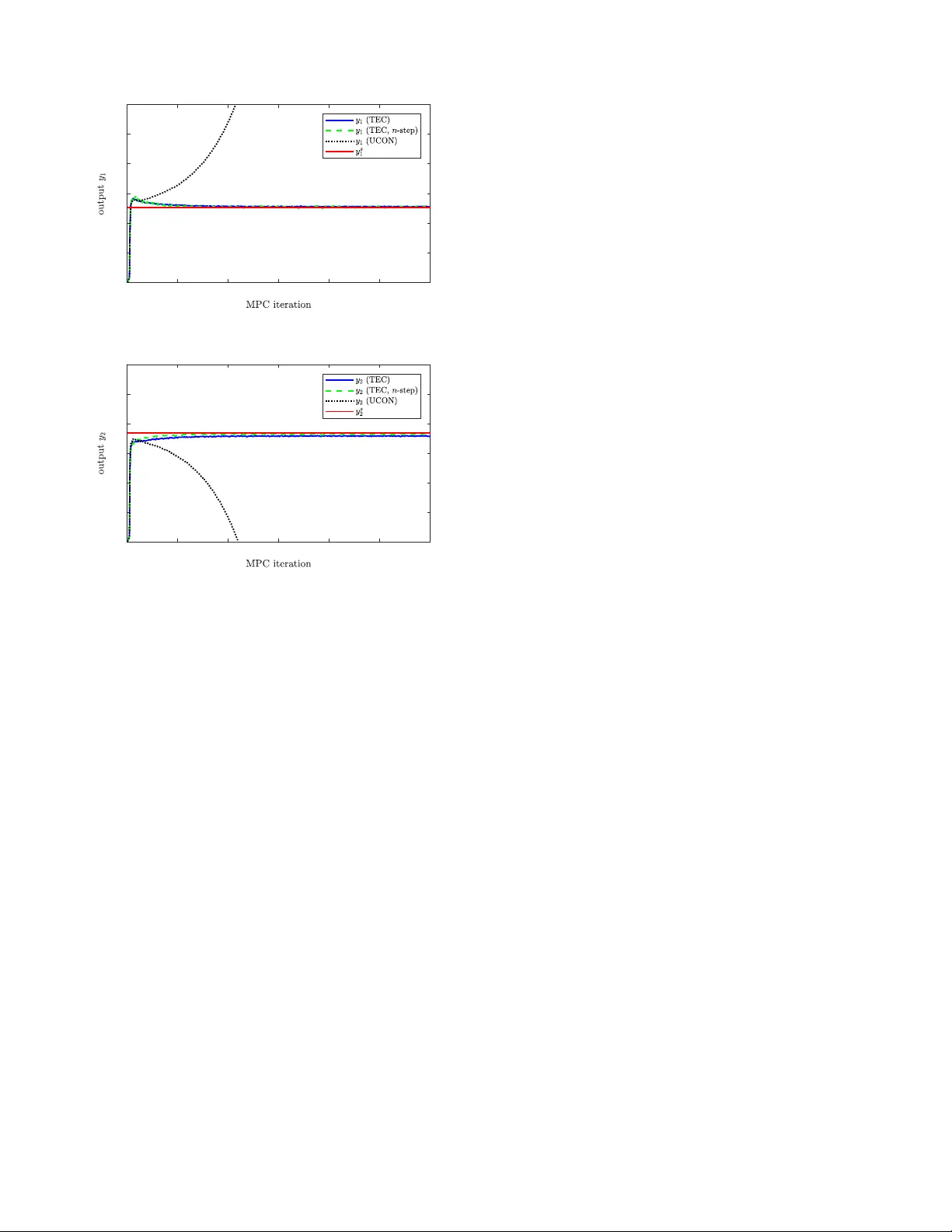
1 Data-Dri v en Model Predicti v e Control with Stability and Rob ustness Guarantees Julian Berberich 1 , Johannes K ¨ ohler 1 , Matthias A. M ¨ uller 2 , and Frank Allg ¨ ower 1 . Abstract —W e propose a robust data-driv en model predictive control (MPC) scheme to control linear time-in variant (L TI) systems. The scheme uses an implicit model description based on behavioral systems theory and past measured trajectories. In particular , it does not requir e any prior identification step, but only an initially measured input-output trajectory as well as an upper bound on the order of the unknown system. First, we prov e exponential stability of a nominal data-driven MPC scheme with terminal equality constraints in the case of no measur ement noise. For bounded additive output measurement noise, we propose a rob ust modification of the scheme, including a slack variable with regularization in the cost. W e pro ve that the application of this rob ust MPC scheme in a multi-step fashion leads to practical exponential stability of the closed loop w .r .t. the noise level. The presented results provide the first (theoretical) analysis of closed- loop properties, resulting from a simple, purely data-driven MPC scheme. Index T erms —Predictive control f or linear systems, data-driven control, uncertain systems, rob ust control. I . I N T RO D U C T I O N While data-dri ven methods for system analysis and control hav e become increasingly popular over the recent years, only few such methods giv e theoretical guarantees on, e.g., stability or constraint satisfaction of system v ariables [1], [2]. A control method, which is naturally well-suited for achieving these objectiv es is model predictive control (MPC), which can handle nonlinear system dynamics, hard constraints on input, state and output, and it takes performance criteria into account [3]. It centers around the repeated online solution of an optimization problem ov er predicted future system trajectories. Thus, for the implementation of MPC, a model of the plant is required, which is usually obtained from first principles or from measured data via system identification [4]. An appealing alternativ e is to implement an MPC controller directly from measured data, without prior knowledge of an accurate model. In various recent works, learning-based or adaptiv e MPC schemes ha ve been proposed, which improve an inaccurate initial model using online measurements [5], [6], [7], [8], [9], This work was funded by Deutsche F orschungsgemeinschaft (DFG, German Research Foundation) under Germany’ s Excellence Strategy - EXC 2075 - 390740016. The authors thank the International Max Planck Research School for Intelligent Systems (IMPRS-IS) for supporting Julian Berberich, and the International Research Training Group Soft Tissue Robotics (GRK 2198/1). 1 Julian Berberich, Johannes K ¨ ohler , and Frank Allg ¨ ower are with the Institute for Systems Theory and Automatic Control, University of Stuttgart, 70550 Stuttgart, Germany (email: { julian.berberich, jo- hannes.koehler , frank.allgower } @ist.uni-stuttgart.de) 2 Matthias A. M ¨ uller is with the Leibniz Uni versity Hannover , Institute of Automatic Control, 30167 Hannover , Germany (e-mail:mueller@irt.uni- hannover .de) while gi ving guarantees on the resulting closed loop. Similarly , MPC based on Gaussian Processes has receiv ed increasing attraction [10], b ut proving desirable closed-loop properties remains an open issue. A different approach, which uses linear combinations of past trajectories to predict future trajectories, has been presented in [11], but also no guarantees on, e.g., stability of the closed loop were gi ven. The design of purely data-driv en MPC approaches with guarantees on stability and constraint satisfaction thus remains an open problem. In this paper , we present a no vel data-dri ven MPC scheme to control linear time-in variant (L TI) systems with stability and robustness guarantees for the closed loop. Our approach relies on a result from behavioral systems theory , which sho ws that the Hankel matrix consisting of a pre viously measured input- output trajectory spans the vector space of all trajectories of an L TI system, given that the input component is persistently ex- citing [12]. Although this result has found various applications in the field of system identification [13], [14], [15], it has only recently been used to develop data-driv en methods for system analysis and control with theoretical guarantees. An exposition of the main result of [12] in the classical state-space control framew ork and an extension to certain classes of nonlinear systems are provided in [16]. Further , the result is employed in [17] to design state- and output-feedback controllers and in [18] to verify dissipation inequalities from measured data, whereas [19] in vestigates data-dri ven control without requiring persistently exciting data. Moreov er , the recent contributions [20], [21], [22] set up an MPC scheme based on [12], but no guarantees on recursi ve feasibility or closed-loop stability can be giv en since neither terminal ingredients are included in the MPC scheme nor sufficient lower bounds on the prediction horizon are deri ved. In the present paper, we propose a related MPC scheme, which utilizes terminal equality constraints, and we provide a theoretical analysis of various desirable properties of the closed loop. T o the best of our kno wledge, this is the first analysis regarding recursi ve feasibility and stability of purely data-driv en MPC. The main advantage of the proposed MPC scheme ov er existing adapti ve or learning-based methods such as [5], [6], [7], [8], [9] is that it requires only an initially measured, persistently exciting data trajectory as well as an upper bound on the system order , but no (set-based) model description and no online estimation process. Moreover , since it relies on the data-driv en system description from [12], the presented scheme is inherently an output-feedback MPC scheme and does not require online state measurements. ©2020 IEEE. Personal use of this material is permitted. Permission from IEEE must be obtained for all other uses, in any current or future media, including reprinting/republishing this material for advertising or promotional purposes, creating new collectiv e works, for resale or redistrib ution to servers or lists, or reuse of any copyrighted component of this work in other works. 2 After stating the required definitions and existing results in Section II, we expand the nominal MPC scheme of [20], [21] by terminal equality constraints in Section III. Under the assumption that the output of the plant can be measured exactly , we prov e recursive feasibility , constraint satisfaction, and exponential stability of the scheme. In Section IV, we propose a robust data-driv en MPC scheme to account for bounded additiv e noise in both the initial data for prediction as well as the online measurements. Under suitable assumptions on the system and design parameters, we prove that the closed loop under application of the scheme in a multi-step fashion leads to a practically e xponentially stable closed loop. In Section V, we illustrate the advantages of the proposed scheme ov er the scheme without terminal constraints from [20], [21], [22] by means of a numerical example. The paper is concluded in Section VI. I I . P R E L I M I NA R I E S Let I [ a,b ] denote the set of inte gers in the interval [ a, b ] . For a vector x and a positiv e definite matrix P = P >  0 , we write k x k P = √ x > P x . Further , we denote the minimal and maximal eigen value of P by λ min ( P ) and λ max ( P ) , respectiv ely . For two matrices P 1 = P > 1 , P 2 = P > 2 , we write λ min ( P 1 , P 2 ) = min { λ min ( P 1 ) , λ min ( P 2 ) } , and similarly for λ max ( P 1 , P 2 ) . Moreover , k x k 2 , k x k 1 , and k x k ∞ denote the Euclidean, ` 1 -, and ` ∞ -norm of x , respecti vely . If the argument is matrix-valued, then we mean the corresponding induced norm. For δ > 0 , we define B δ = { x ∈ R n | k x k 2 ≤ δ } . A sequence { x k } N − 1 k =0 induces the Hankel matrix H L ( x ) : =      x 0 x 1 . . . x N − L x 1 x 2 . . . x N − L +1 . . . . . . . . . . . . x L − 1 x L . . . x N − 1      . For a stacked window of the sequence, we write x [ a,b ] =    x a . . . x b    . W e denote by x either the sequence itself or the stacked vector x [0 ,N − 1] containing all of its components. W e consider the following standard definition of persistence of excitation. Definition 1. W e say that a sequence { u k } N − 1 k =0 with u k ∈ R m is persistently exciting of order L if rank ( H L ( u )) = mL . Our goal is to control an unknown L TI system, denoted by G , of order n with m inputs and p outputs, using only measured input-output data. Definition 2. W e say that an input-output sequence { u k , y k } N − 1 k =0 is a trajectory of an LTI system G , if there exists an initial condition ¯ x ∈ R n as well as a state sequence { x k } N k =0 such that x k +1 = Ax k + B u k , x 0 = ¯ x, y k = C x k + D u k , for k = 0 , . . . , N − 1 , wher e ( A, B , C , D ) is a minimal r ealization of G . Note that we define a trajectory of an L TI system as an input-output sequence that can be produced by a minimal realization, entailing controllability and observability of the system. Extending the results of this paper to systems whose input-output behavior cannot be explained via a minimal real- ization is an interesting issue for future research. The follo wing result lays the foundation of the present paper . It shows that a Hankel matrix, in volving a single persistently exciting trajectory , spans the vector space of all system trajectories of an L TI system. The result originates from beha vioral systems theory [12], but we employ the formulation in the classical state-space control framew ork [16]. Theorem 1 ([16]) . Suppose { u d k , y d k } N − 1 k =0 is a trajectory of an LTI system G , wher e u d is persistently exciting of order L + n . Then, { ¯ u k , ¯ y k } L − 1 k =0 is a trajectory of G if and only if ther e e xists α ∈ R N − L +1 such that  H L ( u d ) H L ( y d )  α =  ¯ u ¯ y  . (1) Recently , Theorem 1 has recei ved increasing attention to dev elop data-driv en controllers [17], verify dissipativity [18], or to design MPC schemes [20], [21], [22]. This is due to the fact that (1) provides an appealing data-dri ven char- acterization of all trajectories of the unknown L TI system, without requiring any prior identification step. In this paper , we use Theorem 1 to develop a data-driv en MPC scheme with pr ovable stability guarantees despite noisy measurements. Note that, if a sequence is persistently exciting of order L , then it is also persistently exciting of order ˜ L for any ˜ L ≤ L . Therefore, Theorem 1 and hence all of our results hold true if n is replaced by a (potentially rough) upper bound. Although we assume that only input-output data of the unknown system are av ailable, we make extensi ve use of the fact that an input-output trajectory of length greater than or equal to n induces a unique internal state in some minimal realization of the unknown system. W e employ MPC to stabilize a desired equilibrium of the system. Since a model of this system is not av ailable, we define an equilibrium via input-output pairs. Definition 3. W e say that an input-output pair ( u s , y s ) ∈ R m + p is an equilibrium of an LTI system G , if the sequence { ¯ u k , ¯ y k } n k =0 with ( ¯ u k , ¯ y k ) = ( u s , y s ) for all k ∈ I [0 ,n ] is a trajectory of G . For an equilibrium ( u s , y s ) , we define u s n and y s n as the column vectors containing n times u s and y s , respectively . W e assume that the system is subject to pointwise-in-time input and output constraints, i.e., u t ∈ U ⊆ R m , y t ∈ Y ⊆ R p for all t ≥ 0 , and we assume ( u s , y s ) ∈ int ( U × Y ) . Throughout this paper,  u d k , y d k  N − 1 k =0 denotes an a priori measured data trajectory of length N , which is used for prediction as in (1). The predicted input- and output-trajectories at time t ov er some prediction horizon L are written as { ¯ u k ( t ) , ¯ y k ( t ) } L − 1 k = − n . Note that the time indices start at k = − n , since the last n inputs and outputs will be used to inv oke a unique initial state 3 at time t . Further, the closed-loop input, the state in some minimal realization, and the output at time t are denoted by u t , x t , and y t , respectiv ely . I I I . N O M I NA L D A TA - D R I VE N M P C In this section, we propose a simple, nominal data-driv en MPC scheme with terminal equality constraints. The scheme relies on noise-free measurements to predict future trajectories using Theorem 1 and is described in Section III-A. Under mild assumptions, we prove recursiv e feasibility , constraint satisfaction, and exponential stability of the closed loop in Section III-B. A. Nominal MPC scheme Commonly , MPC relies on a model of the plant to predict future trajectories and to optimize over them. Theorem 1 provides an appealing alternativ e to a model since (1) suffices to capture all system trajectories. Thus, to implement a data- driv en MPC scheme, one can simply replace the system dynamics constraint by the constraint that the predicted input- output trajectories satisfy (1). T o be more precise, the proposed data-driv en MPC scheme minimizes, at time t , giv en the last n input-output pairs, the following open-loop cost J L ( u [ t − n,t − 1] , y [ t − n,t − 1] ,α ( t )) = L − 1 X k =0 ` ( ¯ u k ( t ) , ¯ y k ( t )) , (2a)  ¯ u [ − n,L − 1] ( t ) ¯ y [ − n,L − 1] ( t )  =  H L + n ( u d ) H L + n ( y d )  α ( t ) , (2b)  ¯ u [ − n, − 1] ( t ) ¯ y [ − n, − 1] ( t )  =  u [ t − n,t − 1] y [ t − n,t − 1]  . (2c) As described above, the constraint (2b) replaces the system dynamics compared to classical model-based MPC schemes. Further , (2c) ensures that the internal state of the true trajectory aligns with the internal state of the predicted trajectory at time t . Note that the overall length of the trajectory ( ¯ u ( t ) , ¯ y ( t )) is L + n since the past n elements { ¯ u k ( t ) , ¯ y k ( t ) } − 1 k = − n are used to specify the initial conditions in (2c). These initial conditions are specified until time step t − 1 , since the input at time t might already influence the output at time t , in case of a feedthrough- element of the plant. The open-loop cost depends only on the decision variable α ( t ) , since ¯ u ( t ) and ¯ y ( t ) are fixed implicitly through the dynamic constraint (2b). Throughout the paper , we consider quadratic stage costs, which penalize the distance w .r .t. a desired equilibrium ( u s , y s ) , i.e., ` ( ¯ u, ¯ y ) = k ¯ u − u s k 2 R + k ¯ y − y s k 2 Q , where Q, R  0 . In [20], [21], it was suggested to directly minimize the abov e open-loop cost subject to constraints on input and output. It is well-kno wn that MPC without terminal constraints requires a sufficiently long prediction horizon to ensure stability and constraint satisfaction [23], [24]. W ith- out such an assumption, the application of MPC can ev en destabilize an open-loop stable system. There are two main approaches in the literature to guarantee stability: a) provid- ing bounds on the minimal required prediction horizon [24] and b) including terminal ingredients such as terminal cost functions or terminal region constraints [25]. Both approaches are usually based on model kno wledge and thus, it is not straightforward to use them in the present, purely data-driven setting. In this paper , we consider a simple terminal equality con- straint, which can be directly included into the data-driv en MPC framework, and which guarantees exponential stability of the closed loop. T o this end, we propose the following data- driv en MPC scheme with a terminal equality constraint. J ∗ L ( u [ t − n,t − 1] , y [ t − n,t − 1] ) = min α ( t ) ¯ u ( t ) , ¯ y ( t ) L − 1 X k =0 ` ( ¯ u k ( t ) , ¯ y k ( t )) (3a) s.t.  ¯ u [ − n,L − 1] ( t ) ¯ y [ − n,L − 1] ( t )  =  H L + n ( u d ) H L + n ( y d )  α ( t ) , (3b)  ¯ u [ − n, − 1] ( t ) ¯ y [ − n, − 1] ( t )  =  u [ t − n,t − 1] y [ t − n,t − 1]  , (3c)  ¯ u [ L − n,L − 1] ( t ) ¯ y [ L − n,L − 1] ( t )  =  u s n y s n  , (3d) ¯ u k ( t ) ∈ U , ¯ y k ( t ) ∈ Y , k ∈ I [0 ,L − 1] . (3e) The terminal equality constraint (3d) implies that ¯ x L ( t ) , which is the internal state predicted L steps ahead corresponding to the predicted input-output trajectory , aligns with the steady- state x s corresponding to ( u s , y s ) , i.e., ¯ x L ( t ) = x s in any minimal realization. While Problem (3) requires that ( u s , y s ) is an equilibrium of the unkno wn system in the sense of Definition 3, this requirement can be dropped when ( u s , y s ) is replaced by an artificial equilibrium, which is also optimized online (compare [26]). The recent paper [27] extends the abov e MPC scheme to such a setting, thereby leading to a significantly larger region of attraction for the closed loop without requiring knowledge of a reachable equilibrium of the unknown system. As in standard MPC, Problem (3) is solved in a receding horizon fashion, which is summarized in Algorithm 1. Algorithm 1. Data-Driven MPC Scheme 1) At time t , take the past n measurements u [ t − n,t − 1] , y [ t − n,t − 1] and solve (3). 2) Apply the input u t = ¯ u ∗ 0 ( t ) . 3) Set t = t + 1 and go back to 1). W ith slight abuse of notation, we will denote the open-loop cost and the optimal open-loop cost of (3) by J L ( x t , α ( t )) and J ∗ L ( x t ) , respectiv ely , where x t is the state in some minimal realization, induced by u [ t − n,t − 1] , y [ t − n,t − 1] . B. Closed-loop guarantees W ithout loss of generality , we assume for the analysis that u s = 0 , y s = 0 , and thus x s = 0 . Further , we define the set of initial states, for which (3) is feasible, by X L = { x ∈ R n | J ∗ L ( x ) < ∞} . T o prov e exponential stability of the proposed scheme, we assume that the optimal value 4 function of (3) is quadratically upper bounded. This is, e.g., satisfied in the present linear-quadratic setting if the constraints are polytopic 1 [28]. Assumption 1. The optimal value function J ∗ L ( x ) is quadrat- ically upper bounded on X L , i.e., ther e exists c u > 0 such that J ∗ L ( x ) ≤ c u k x k 2 2 for all x ∈ X L . Moreov er , we assume that the input u d generating the data used for prediction is sufficiently rich in the follo wing sense. Assumption 2. The input u d of the data trajectory is persis- tently exciting of or der L + 2 n . Note that we assume persistence of e xcitation of order L + 2 n , although Theorem 1 requires only an order of L + n . This is due to the fact that the reconstructed trajectories in (3) are of length L + n (compared to length L in Theorem 1), since n components are used to fix the initial conditions. Furthermore, due to the terminal constraints (3d), the prediction horizon needs to be at least as long as the system order n . Assumption 3. The pr ediction horizon satisfies L ≥ n . The following result shows that the MPC scheme based on (3) is recursi vely feasible, ensures constraint satisfaction, and leads to an exponentially stable closed loop. Theorem 2. Suppose Assumptions 1, 2 and 3 are satisfied. If the MPC pr oblem (3) is feasible at initial time t = 0 , then (i) it is feasible at any t ∈ N , (ii) the closed loop satisfies the constraints, i.e., u t ∈ U and y t ∈ Y for all t ∈ N , (iii) the equilibrium x s = 0 is e xponentially stable for the r esulting closed loop. Pr oof. Recursiv e feasibility (i) and constraint satisfaction (ii) follow from standard MPC ar guments, i.e., by defining a candidate solution as the shifted, pre viously optimal solution and appending zero (compare [3]). (iii). Exponential Stability Denote the standard candidate solution mentioned above by ¯ u 0 ( t + 1) , ¯ y 0 ( t + 1) , α 0 ( t + 1) . The cost of this solution is J L ( x t +1 , α 0 ( t + 1)) = L − 1 X k =0 ` ( ¯ u 0 k ( t + 1) , ¯ y 0 k ( t + 1)) = L − 1 X k =1 ` ( ¯ u ∗ k ( t ) , ¯ y ∗ k ( t )) = J ∗ L ( x t ) − ` ( ¯ u ∗ 0 ( t ) , ¯ y ∗ 0 ( t )) . Hence, it holds that J ∗ L ( x t +1 ) ≤ J ∗ L ( x t ) − ` ( ¯ u ∗ 0 ( t ) , ¯ y ∗ 0 ( t )) . (4) Since x is the state of an observ able (and hence detectable) minimal realization, there exists a matrix P  0 such that 1 While [28] considered model-based linear-quadratic MPC, the result applies similarly to the present data-driven MPC setting since (3b) (together with the initial conditions (3c)) describes the input-output behavior of the system exactly and thus, both settings are equivalent in the nominal case. W ( x ) = k x k 2 P is an input-output-to-state stability (IOSS) L yapunov function 2 , which satisfies W ( Ax + B u ) − W ( x ) ≤ − 1 2 k x k 2 2 + c 1 k u k 2 2 + c 2 k y k 2 2 , (5) for all x ∈ R n , u ∈ R m , y = C x + Du , and for suitable c 1 , c 2 > 0 [29]. Define the candidate L yapunov function V ( x ) = γ W ( x ) + J ∗ L ( x ) for some γ > 0 . Note that V is quadratically lower bounded, i.e., V ( x ) ≥ γ W ( x ) ≥ γ λ min ( P ) k x k 2 2 for all x ∈ X L . Further , J ∗ L is quadratically upper bounded by Assumption 1, i.e., J ∗ L ( x ) ≤ c u k x k 2 2 for all x ∈ X L . Hence, we hav e V ( x ) = J ∗ L ( x ) + γ W ( x ) ≤ ( c u + γ λ max ( P )) k x k 2 2 , for all x ∈ X L , i.e., V is quadratically upper bounded. W e consider now γ = λ min ( Q, R ) max { c 1 , c 2 } > 0 . Along the closed-loop trajectories, using both (4) as well as (5), it holds that V ( x t +1 ) − V ( x t ) ≤ γ  − 1 2 k x t k 2 2 + c 1 k u t k 2 2 + c 2 k y t k 2 2  − k u t k 2 R − k y t k 2 Q ≤ − γ 2 k x t k 2 2 . It follo ws from standard L yapunov arguments with L yapunov function V that the equilibrium x s = 0 is exponentially stable with region of attraction X L . The proof of Theorem 2 applies standard arguments from model-based MPC with terminal constraints (compare [3]) to the data-dri ven system description deriv ed in [12], similar to the approaches of [20], [21] which did howe ver not address closed-loop guarantees. T o handle the fact that the stage cost ` is merely positi ve semi -definite in the state, detectability of the stage cost is exploited via an IOSS L yapunov function [29], similar to [30]. As we will see in Section IV, this analogy between model-based MPC and the proposed data-dri ven MPC scheme is only present in the nominal case, where the data is noise-free. For the more realistic case of noisy output measurements, we de velop a robust data-driv en MPC scheme and we provide a novel theoretical analysis of the closed loop in Section IV, which is the main contribution of this paper . Remark 1. W e would like to emphasize the simplicity of the pr oposed MPC scheme . W ithout any prior identification step, a single measur ed data trajectory can be used directly to set up an MPC scheme for a linear system. Compar ed to other learning-based MPC appr oaches such as [5], [6], [7], [8], [9], which r equir e initial model knowledge as well as an online estimation pr ocess, the complexity of (3) is similar to classical MPC schemes, which r ely on full model knowledge. T o be mor e pr ecise, the decision variables ¯ u ( t ) , ¯ y ( t ) can be r eplaced by α ( t ) via (3b) (using a condensed formulation) 2 Note that, in [29, Section 3.2], only strictly proper systems with y = C x are considered, while we allow for more general systems with y = C x + D u . The result from [29] can be extended to y = C x + D u by considering a modified ˜ B = B + LD in [29, Inequality (12)]. 5 and hence, since α ( t ) ∈ R N − L − n +1 , Pr oblem (3) contains in total N − L − n + 1 decision variables. F or u d to be persistently exciting of or der L + 2 n , it needs to hold that N − L − 2 n + 1 ≥ m ( L + 2 n ) . Assuming equality , Pr oblem (3) hence has m ( L + 2 n ) + n free parameters. On the contrary , a condensed model-based MPC optimization pr oblem contains mL decision variables for the input trajectory (assuming that state measur ements ar e available). Thus, the online complexity of the pr oposed data-driven MPC approac h is slightly lar ger ( 2 mn + n additional decision variables) than that of model- based MPC, but it does not r equire an a priori (offline) identification step. It is worth noting that the differ ence in complexity is independent of the horizon L . Moreo ver , the pr oposed data-driven MPC is inher ently an output-feedback contr oller since no state measur ements are r equir ed for its implementation. F inally , as in model-based MPC, for con vex polytopic (or quadratic) constraints U , Y , (3) is a conve x (quadratically constrained) quadratic pr ogram which can be solved efficiently . I V . R O BU S T DAT A - D R I V E N M P C In this section, we propose a multi-step robust data-dri ven MPC scheme and we prov e practical exponential stability of the closed loop in the presence of bounded additiv e output measurement noise. The scheme includes a slack variable, which is regularized in the cost and compensates noise both in the initial data ( u d , y d ) used for prediction and in the online measurement updates  u [ t − n,t − 1] , y [ t − n,t − 1]  . Section IV -A contains the scheme, which is essentially a robust modification of the nominal scheme of Section III, as well as detailed explanations of the key ingredients. In Sections IV -B and IV -C, we prove two technical Lemmas, which will be required for our main theoretical results. Recursiv e feasibility of the closed loop is proven in Section IV -D. In Section IV -E, we show that, under suitable assumptions, the closed loop resulting from the application of the multi-step MPC scheme leads to a practically exponentially stable closed loop. Moreover , if the noise bound tends to zero, then the region of attraction of the closed loop approaches the set of all initially feasible points. In this section, we do not consider output constraints, i.e., Y = R p . In [31], we recently extended the results of this section by incorporating tightened output constraints in order to guarantee closed-loop constraint satisfaction despite noisy data. A. Robust MPC scheme In practice, the output of the unknown L TI system G is usu- ally not av ailable exactly , but might be subject to measurement noise. This implies that the stacked data-dependent Hankel matrices in (1) do not span the system’ s trajectory space exactly and thus, the output trajectories cannot be predicted accurately . Moreov er , noisy output measurements enter the initial conditions in Problem (3), which deteriorates the pre- diction accuracy ev en further . Therefore, a direct application of the MPC scheme of Section III may lead to feasibility issues or it may render the closed loop unstable. In this section, we tackle the issue of noisy measurements with a robust data-dri ven MPC scheme with terminal constraints. W e consider output measurements with bounded additive noise in the initially a vailable data ˜ y d k = y d k + ε d k as well as in the online measurements ˜ y k = y k + ε k . W e make no assumptions on the nature of the noise, but we require that it is bounded as k ε d k k ∞ ≤ ¯ ε and k ε k k ∞ ≤ ¯ ε for some ¯ ε > 0 . Thus, the present setting includes two types of noise. The data used for the prediction via the Hankel matrices in (1) is perturbed by ε d , which can thus be interpreted as a multiplicativ e model uncertainty . On the other hand, ε perturbs the online measurements and hence, the overall control goal is a noisy output-feedback problem. The key idea to account for noisy measurements is to relax the equality constraint (3b), where the relaxation parameter is penalized appropriately in the cost function. Gi ven a noisy initial input-output trajectory  u [ t − n,t − 1] , ˜ y [ t − n,t − 1]  of length n , and noisy data ( u d , ˜ y d ) , we propose the following robust modification of (3). J ∗ L  u [ t − n,t − 1] , ˜ y [ t − n,t − 1]  = min α ( t ) ,σ ( t ) ¯ u ( t ) , ¯ y ( t ) L − 1 X k =0 ` ( ¯ u k ( t ) , ¯ y k ( t )) + λ α ¯ ε k α ( t ) k 2 2 + λ σ k σ ( t ) k 2 2 s.t.  ¯ u ( t ) ¯ y ( t ) + σ ( t )  =  H L + n  u d  H L + n  ˜ y d   α ( t ) , (6a)  ¯ u [ − n, − 1] ( t ) ¯ y [ − n, − 1] ( t )  =  u [ t − n,t − 1] ˜ y [ t − n,t − 1]  , (6b)  ¯ u [ L − n,L − 1] ( t ) ¯ y [ L − n,L − 1] ( t )  =  u s n y s n  , ¯ u k ( t ) ∈ U , (6c) k σ k ( t ) k ∞ ≤ ¯ ε (1 + k α ( t ) k 1 ) , k ∈ I [0 ,L − 1] . (6d) Compared to the nominal MPC problem (3), the output data trajectory ˜ y d as well as the initial output ˜ y [ t − n,t − 1] , which is obtained via online measurements, have been replaced by their noisy counterparts. Further , the following ingredients have been added: a) A slack variable σ , bounded by (6d), to account for the noisy online measurements ˜ y [ t − n,t − 1] and for the noisy data ˜ y d used for prediction, which can be interpreted as a multiplicativ e model uncertainty , b) Quadratic regularization (i.e., ridge r e gularization ) of α and σ with weights λ α ¯ ε, λ σ > 0 , i.e., the regularization of α depends on the noise level. The above ` 2 -norm regularization for α ( t ) implies that small values of k α ( t ) k 2 2 are preferred. Since the noisy Hankel matrix H L + n  ˜ y d  is multiplied by α ( t ) in (6a), this implicitly reduces the influence of the noise on the prediction accuracy . Intuitiv ely , for increasing λ α , the term λ α ¯ ε k α ( t ) k 2 2 reduces the “complexity” of the data-driven system description (6a), simi- lar to regularization methods in linear re gression, thus allo wing for a tradeoff between tracking performance and the av oidance of ov erfitting. The term λ σ k σ ( t ) k 2 2 yields small values for the slack v ariable σ ( t ) , thus improving the prediction accuracy . For our theoretical results, λ σ can be chosen to be zero since σ ( t ) is already rendered small by the constraint (6d). Ho wev er , as we discuss in more detail in Remark 3, the constraint (6d) is non-con vex but can be neglected if λ σ is large enough. 6 An alternativ e to the present regularization terms are gen- eral quadratic regularization kernels, i.e., costs of the form k α ( t ) k 2 P α , k σ ( t ) k 2 P σ for suitable matrices P α , P σ  0 . Further , in [21], [22], ` 1 -regularizations of α and σ were suggested and the resulting MPC scheme, without terminal equality constraints, was successfully applied to a nonlinear stochastic control problem. Howe ver , theoretical guarantees on closed- loop stability were not given. Throughout this paper , we consider simple quadratic penalty terms since this simplifies the arguments, but we conjecture that our theoretical results remain to hold for general norms k α ( t ) k p , k σ ( t ) k q with ar- bitrary p, q = 1 , . . . , ∞ . An interesting open question, which is beyond the scope of this paper, is to in vestigate the impact of particular choices of regularization norms on the practical performance of the presented MPC approach. The choice of norms in the constraint (6d) is independent of the norms in the cost and essentially follows from the ` ∞ -noise bound and the proofs of the v alue function upper bound (Lemma 1) and recursiv e feasibility (Proposition 1). In this section, we study the closed loop resulting from an application of (6) in an n -step MPC scheme (compare [32], [33]). T o be more precise, we consider the scenario that, after solving (6) online, the first n computed inputs are applied to the system. Thereafter , the horizon is shifted by n steps, before the whole scheme is repeated (compare Algorithm 2). Algorithm 2. n -Step Data-Driven MPC Scheme 1) At time t , take the past n measurements u [ t − n,t − 1] , ˜ y [ t − n,t − 1] and solve (6). 2) Apply the input sequence u [ t,t + n − 1] = ¯ u ∗ [0 ,n − 1] ( t ) over the next n time steps. 3) Set t = t + n and go back to 1). As we will see in the remainder of this section, for the considered setting with output measurement noise, the multi- step MPC scheme described in Algorithm 2 has superior theo- retical properties compared to its corresponding 1 -step version. This is mainly due to the terminal equality constraints (6c), which complicate the proof of recursiv e feasibility , similar as in model-based robust MPC with terminal equality constraints and model mismatch. In particular , we show in this section that, for an n -step MPC scheme with a terminal equality constraint, practical exponential stability can be proven. On the other hand, we comment on the differences for the corre- sponding 1 -step MPC scheme in Section IV -D (Remark 4). In particular , for a 1 -step MPC scheme relying on (6), recursiv e feasibility holds only locally around ( u s , y s ) and thus, only local stability can be guaranteed. Nev ertheless, as we will see in Section V for a numerical example, the practical performance of the n -step scheme is almost indistinguishable from the 1 -step scheme. Remark 2. In the nominal case of Section III, i.e., for ¯ ε = 0 , (6d) implies σ = 0 . Further , the r e gularization of α vanishes for ¯ ε = 0 , and the system dynamics (6a) as well as the initial conditions (6b) approac h their nominal counterparts. Thus, for ¯ ε = 0 , Pr oblem (6) reduces to the nominal Pr oblem (3) . Remark 3. If the constraint (6d) is ne glected and the input constraint set U is a conve x polytope , then Pr oblem (6) is a strictly conve x quadratic pr ogram and can be solved efficiently . However , the constraint on the slack variable σ in (6d) is non-con vex due to the dependence of the right-hand side on k α ( t ) k 1 , making it difficult to implement (6) in an efficient way . As will become clear later in this section, (6d) is requir ed to pr ove r ecursive feasibility and practical e xpo- nential stability . It may , however , be r eplaced by the (con vex) constraint k σ k ( t ) k ∞ ≤ c · ¯ ε for a sufficiently larg e constant c > 0 , r etaining the same theoretical guarantees. Generally , a larger choice of c increases the r egion of attraction, but also the size of the exponentially stable set to whic h the closed loop con ver ges. Furthermor e, the constr aint (6d) can be enfor ced implicitly by choosing λ σ lar ge enough. In simulation examples, it was observed that the constraint (6d) is usually satisfied (for suitably lar ge choices of λ σ ) without enforcing it explicitly in the optimization pr oblem and thus, it may in most cases be ne glected in the online optimization. As in the pre vious section, we require that the measured input u d is persistently exciting of order L + 2 n (Assump- tion 2). Further , to establish a local upper bound on the optimal cost of (6) and to prove recursive feasibility , we require that the horizon L is not shorter than twice the system’ s order , as captured in the following assumption. Assumption 4. The pr ediction horizon satisfies L ≥ 2 n . In some minimal realization, we denote the state trajectory corresponding to ( u d , y d ) by x d . According to [12, Corollary 2], Assumption 2 implies that the matrix H ux = " H L + n  u d  H 1  x d [0 ,N − L − n ]  # (7) has full row rank and thus admits a right-in verse H † ux = H > ux  H ux H > ux  − 1 . Define the quantity c pe : =   H † ux   2 2 . (8) For our stability results, we will require that c pe ¯ ε is bounded from above by a sufficiently small number . Essentially , this corresponds to a quantitative “persistence-of-excitation-to- noise”-bound. T o be more precise, abbreviate in the following U = H L + n ( u d ) and suppose that ρI m ( L + n )  U U >  ν I m ( L + n ) (9) for scalar constants ρ, ν > 0 . Further , define the quantity c u pe = k U † k 2 2 = k U > ( U U > ) − 1 k 2 2 . Then, it holds that c u pe ≤   U >   2 2     U U >  − 1    2 2 (10) = λ max ( U U > ) · λ max  ( U U > ) − 1 ( U U > ) − 1  ≤ λ max ( U U > ) λ min ( U U > ) 2 (9) ≤ ν ρ 2 . Thus, if a persistently exciting input u d is multiplied by a constant c > 1 , then c u pe decreases proportionally to 1 c 2 . Further , the constant ρ can typically be chosen larger if the data length N increases. The same arguments can be carried 7 out when assuming a bound of the form (9) for the matrix (7), but finding a suitable input which generates data achie ving such a bound is less obvious. It is well-known for classical definitions of persistence of excitation that larger excitation of the input implies larger excitation of the state. Therefore, we conjecture (and we hav e observed for various practical simulation examples) that c pe decreases with increasing data horizons N and with multiplications of a persistently exciting input data trajectory u d by a scalar constant greater than one. This means that, for a given noise le vel ¯ ε , robust stability as guaranteed in the follo wing sections can be obtained by choosing a large enough persistently exciting input u d and/or a sufficiently large data horizon N . Similar to Section III, we denote the open- loop cost of the robust MPC problem (6) by J L  u [ t − n,t − 1] , ˜ y [ t − n,t − 1] , α ( t ) , σ ( t )  , and the optimal cost by J ∗ L  u [ t − n,t − 1] , ˜ y [ t − n,t − 1]  . Moreover , we assume for the analysis that ( u s , y s ) = (0 , 0) . For the presented robust data-driv en MPC scheme, setpoints ( u s , y s ) 6 = (0 , 0) change mainly one quantitati ve constant in Lemma 1. W e comment on the main differences in the case ( u s , y s ) 6 = (0 , 0) in Section IV -D (Remark 5). B. Local upper bound of L yapunov function In this section, we show that the optimal cost of (6) admits a quadratic upper bound, similar to the nominal case (cf. Assumption 1). It is straightforward to see that such an upper bound can not be quadratic in the state x of some minimal realization: the optimal cost J ∗ L depends expl icitly on α ∗ ( t ) via λ α ¯ ε k α ∗ ( t ) k 2 2 , which in turn depends on the past n inputs and outputs ( u [ t − n,t − 1] , y [ t − n,t − 1] ) through (6a) and (6b). Even if the current state is zero, i.e., x t = 0 , these may in general be arbitrarily large and hence, α and therefore also J ∗ L may be arbitrarily large. Thus, J ∗ L does not admit an upper bound in the state x t of a minimal realization. T o overcome this issue, we consider a dif ferent (not minimal) state of the system, defined as ξ t : =  u [ t − n,t − 1] y [ t − n,t − 1]  . Further , we define the noisy version of ξ as ˜ ξ t : =  u [ t − n,t − 1] ˜ y [ t − n,t − 1]  =  u [ t − n,t − 1] y [ t − n,t − 1] + ε [ t − n,t − 1]  . Denote the (not inv ertible) linear transformation from ξ to an arbitrary but fixed state x in some minimal realization by T , i.e., x t = T ξ t . Clearly , this implies k x t k 2 2 ≤ k T k 2 2 k ξ t k 2 2 = : Γ x k ξ t k 2 2 . Note that ξ is the state of a detectable state-space realization and thus, there exists an IOSS L yapunov function W ( ξ ) = k ξ k 2 P , similar to the proof of Theorem 2. For some γ > 0 , define V t : = J ∗ L ( ˜ ξ t ) + γ W ( ξ t ) . The following result shows that, for the state ξ , a meaningful quadratic upper bound on V can be pro ven. Lemma 1. Suppose Assumptions 2 and 4 hold. Then, ther e exists a constant c 3 > 0 as well as a δ > 0 suc h that, for all ξ t ∈ B δ , Pr oblem (6) is feasible and V is bounded as γ λ min ( P ) k ξ t k 2 2 ≤ V t ≤ c 3 k ξ t k 2 2 + c 4 , (11) wher e c 4 = 2 np ¯ ε 2 λ σ . Pr oof. The lower bound is trivial. For the upper bound, we construct a feasible candidate solution to Problem (6) which brings the state x in some minimal realization (and thus the output y ) to zero in L steps. Obviously , we have ¯ u [ − n, − 1] ( t ) = u [ t − n,t − 1] as well as ¯ y [ − n, − 1] ( t ) = ˜ y [ t − n,t − 1] by (6b). By assumption, we have L ≥ 2 n as well as 0 ∈ int ( U ) . Thus, by controllability , there exists a δ > 0 such that for any x t with 1 Γ x k x t k 2 ≤ k ξ t k 2 ≤ δ , there exists an input trajectory u [ t,t + L − 1] ∈ U L , which brings the state x [ t,t + L − 1] and the corresponding output y [ t,t + L − 1] to the origin in L − n steps while satisfying      u [ t,t + L − 1] y [ t,t + L − 1]      2 2 ≤ Γ uy k x t k 2 2 (12) for a suitable constant Γ uy > 0 . As candidate input-output trajectories for (6), we choose these u, y , i.e., ¯ u [0 ,L − 1] ( t ) = u [ t,t + L − 1] , ¯ y [0 ,L − 1] ( t ) = y [ t,t + L − 1] . Moreov er, α ( t ) is chosen as α ( t ) = H † ux  u [ t − n,t + L − 1] x t − n  , (13) where H ux is defined in (7). As is described in more detail in [15], [16], the output of an L TI system is a linear combi- nation of its initial condition and the input, and therefore, the abov e choice of α ( t ) implies  H L + n  u d  H L + n  y d   α ( t ) =  ¯ u [ − n,L − 1] ( t ) y [ t − n,t + L − 1]  =   ¯ u [ − n,L − 1] ( t ) ¯ y [ − n, − 1] ( t ) − ε [ t − n,t − 1] ¯ y [0 ,L − 1] ( t )   , where ε [ t − n,t − 1] is the true noise instance. For the slack variable σ , we choose σ [ − n, − 1] ( t ) = H n  ε d [0 ,N − L − 1]  α ( t ) − ε [ t − n,t − 1] , σ [0 ,L − 1] ( t ) = H L  ε d [ n,N − 1]  α ( t ) , (14) which implies that (6a)-(6c) are satisfied. Finally , writing e i for a row vector whose i -th component is equal to 1 and which is zero otherwise, we obtain k H L + n ( ε d ) α ( t ) k ∞ = max i ∈ I [1 ,p ( L + n )] | e i H L + n ( ε d ) α ( t ) | ≤ ¯ ε k α ( t ) k 1 . (15) This implies k σ ( t ) k ∞ ≤ ¯ ε ( k α ( t ) k 1 + 1) , which in turn prov es that (6d) is satisfied. In the following, we employ the above candidate solution to bound the optimal cost and thereby , the function V . Due to observability of the pair ( A, C ) , corresponding to the minimal realization with state x , it holds that  ¯ u [ − n, − 1] ( t ) x t − n  =  I mn 0 M 1 Φ †  | {z } M : = ξ t , (16) where Φ † = (Φ > Φ) − 1 Φ > is a left-inv erse of the observability matrix Φ . The lo wer block of (16) follo ws from observability 8 and the linear system dynamics x k +1 = Ax k + B u k , y k = C x k + D u k for k ∈ I [ t − n,t − 1] , which can be used to compute the matrix M 1 depending on A, B , C , D . Hence, α ( t ) can be bounded as k α ( t ) k 2 2 (13) ≤   H † ux   2 2    ¯ u [ − n,L − 1] ( t )   2 2 + k x t − n k 2 2  =   H † ux   2 2   ¯ u [0 ,L − 1] ( t )   2 2 +      ¯ u [ − n, − 1] ( t ) x t − n      2 2 ! (12) , (16) ≤   H † ux   2 2 | {z } c pe =  Γ uy k x t k 2 2 + k M k 2 2 k ξ t k 2 2  . (17) Using standard norm equi valence properties, it holds for arbitrary k ∈ N that    H k  ε d [0 ,N − L − n + k − 1]     2 2 ≤ c 5 k ¯ ε 2 , (18) where c 5 : = p ( N − L − n + 1) . Based on the definition of σ ( t ) in (14), and using (18) as well as the inequality ( a + b ) 2 ≤ 2( a 2 + b 2 ) , we can bound σ ( t ) in terms of α ( t ) as k σ ( t ) k 2 2 ≤ 2 np ¯ ε 2 + c 5 ( L + 2 n ) ¯ ε 2 k α ( t ) k 2 2 . (19) Combining the above inequalities, V is upper bounded as V t ≤ J L ( ˜ ξ t , α ( t ) , σ ( t )) + γ W ( ξ t ) ≤ λ max ( Q, R )Γ uy k x t k 2 2 + γ λ max ( P ) k ξ t k 2 2 + ( λ α + c 5 ( L + 2 n ) λ σ ¯ ε ) c pe ¯ ε  Γ uy k x t k 2 2 + k M k 2 2 k ξ t k 2 2  + 2 np ¯ ε 2 λ σ . Finally , x t is bounded by ξ t as k x t k 2 2 ≤ Γ x k ξ t k 2 2 , which leads to V t ≤ c 3 k ξ t k 2 2 + c 4 , where c 3 = λ max ( Q, R )Γ uy Γ x + γ λ max ( P ) + ( λ α + c 5 ( L + 2 n ) λ σ ¯ ε ) c pe ¯ ε  Γ uy Γ x + k M k 2 2  , c 4 = 2 np ¯ ε 2 λ σ . In Section III, we assumed that the optimal cost is quadrat- ically upper bounded (cf. Assumption 1), which is not restric- tiv e in the nominal linear-quadratic setting. Lemma 1 prov es that, under mild assumptions, the optimal cost of the robust MPC problem (6) admits (locally) a similar upper bound and can thus be seen as the robust counterpart of Assumption 1. The term c 4 is solely due to the slack v ariable σ . This can be explained by noting that, for ξ t = 0 , α ( t ) , ¯ u [0 ,L − 1] ( t ) , ¯ y [0 ,L − 1] ( t ) can all be chosen to be zero, as long as σ compensates the noise, i.e., σ [ − n, − 1] ( t ) = − ε [ t − n,t − 1] . C. Prediction err or bound Denote the optimizers of (6) by α ∗ ( t ) , σ ∗ ( t ) , ¯ u ∗ ( t ) , ¯ y ∗ ( t ) , and the output trajectory resulting from an open-loop applica- tion of ¯ u ∗ ( t ) by ˆ y . One of the reasons why it is difficult to analyze the presented MPC scheme is the non-trivial relation between the predicted output ¯ y ∗ ( t ) and the “actual” output ˆ y . In the following, we deriv e a bound on the difference between the two quantities, which will play an important role in proving recursiv e feasibility and practical stabiliy of the proposed scheme. For an integer k , define constants ρ 2 ,k , ρ ∞ ,k such that ρ 2 ,k ≥   C A k Φ †   2 2 , ρ ∞ ,k ≥   C A k Φ †   ∞ , where Φ † is a left-in verse of the observ ability matrix Φ . Lemma 2. If (6) is feasible at time t , then the following inequalities hold for all k ∈ I [0 ,L − 1] k ˆ y t + k − ¯ y ∗ k ( t ) k 2 2 ≤ 8 c 5 ¯ ε 2 k α ∗ ( t ) k 2 2 + 2 k σ ∗ k ( t ) k 2 2 (20) + ρ 2 ,n + k  16 n ¯ ε 2  c 5 k α ∗ ( t ) k 2 2 + p  + 4 k σ ∗ [ − n, − 1] ( t ) k 2 2  , k ˆ y t + k − ¯ y ∗ k ( t ) k ∞ ≤ ¯ ε k α ∗ ( t ) k 1 + k σ ∗ k ( t ) k ∞ (21) + ρ ∞ ,n + k  ¯ ε ( k α ∗ ( t ) k 1 + 1) +    σ ∗ [ − n, − 1] ( t )    ∞  , with c 5 fr om (18) . Pr oof. W e sho w only (21) and note that (20) can be deri ved following the same steps, using (18) as well as the inequality ( a + b ) 2 ≤ 2 a 2 + 2 b 2 . As written above, ˆ y is the trajec- tory , resulting from an open-loop application of ¯ u ∗ ( t ) and with initial conditions specified by  u [ t − n,t − 1] , ˆ y [ t − n,t − 1]  =  u [ t − n,t − 1] , y [ t − n,t − 1]  . On the other hand, according to (6a), ¯ y ∗ ( t ) is comprised as ¯ y ∗ ( t ) = H L + n  ε d  α ∗ ( t ) + H L + n  y d  α ∗ ( t ) − σ ∗ ( t ) . It follows directly from (6a) and (6b) that the second term on the right-hand side H L + n  y d  α ∗ ( t ) is a trajectory of G , resulting from an open-loop application of ¯ u ∗ ( t ) and with initial output conditions ˜ y [ t − n,t − 1] + σ ∗ [ − n, − 1] ( t ) − H n  ε d [0 ,N − L − 1]  α ∗ ( t ) . Define y − [ t − n,t + L − 1] = ˆ y [ t − n,t + L − 1] − H L + n  y d  α ∗ ( t ) . Since G is L TI and y − contains the dif ference between two trajectories with the same input, we can assume ¯ u ∗ ( t ) = 0 for the following arguments without loss of generality . Hence, y − is equal to the output component of a trajectory ( u − , y − ) with zero input and with initial trajectory " u − [ t − n,t − 1] y − [ t − n,t − 1] # = (22) " 0 H n  ε d [0 ,N − L − 1]  α ∗ ( t ) − ε [ t − n,t − 1] − σ ∗ [ − n, − 1] ( t ) # . The relation to the internal state x − can be deriv ed as y − [ t − n,t − 1] = Φ x − t − n , with the observability matrix Φ . This leads to the correspond- ing output at time t + k y − t + k = C A n + k Φ † y − [ t − n,t − 1] , where Φ † is a left-in verse of Φ . Using this fact, the expression for y − [ t − n,t − 1] in (22), and the inequality (15), k y − t + k k ∞ can be bounded as k y − t + k k ∞ ≤ ρ ∞ ,n + k  ¯ ε ( k α ∗ ( t ) k 1 + 1) +    σ ∗ [ − n, − 1] ( t )    ∞  . 9 Note that k ˆ y t + k − ¯ y ∗ k ( t ) k ∞ ≤ k y − t + k k ∞ + ¯ ε k α ∗ ( t ) k 1 + k σ ∗ k ( t ) k ∞ , which concludes the proof. Essentially , Lemma 2 giv es a bound on the mismatch between the predicted output and the actual output resulting from the open-loop application of ¯ u ∗ ( t ) , depending on the optimal solutions α ∗ , σ ∗ , and on system parameters. In model- based robust MPC schemes, similar bounds are typically used to propagate uncertainty , where the role of the weighting vector α to account for multiplicative uncertainty is replaced by the state x and a model-based uncertainty description (compare [34] for details). The main dif ference in the proposed MPC scheme is that the predicted trajectory ¯ y ∗ ( t ) is in general not a trajectory of the system in the sense of Definition 2, corresponding to the input ¯ u ∗ ( t ) . On the contrary , in model- based robust MPC, the predicted trajectory usually satisfies the dynamics of a (nominal) model of the system. D. Recursive feasibility The follo wing result shows that, if the proposed rob ust MPC scheme is feasible at time t , then it is also feasible at time t + n , assuming that the noise lev el is sufficiently small. Proposition 1. Suppose Assumption 2 and 4 hold. Then, for any V RO A > 0 , ther e exists an ¯ ε 0 > 0 such that for all ¯ ε ≤ ¯ ε 0 , if V t ≤ V RO A for some t ≥ 0 , then the optimization pr oblem (6) is feasible at time t + n . Pr oof. Suppose the robust MPC problem (6) is feasible at time t with V t ≤ V RO A and denote the optimizers by α ∗ ( t ) , σ ∗ ( t ) , ¯ u ∗ ( t ) , ¯ y ∗ ( t ) . As in Lemma 2, the trajectory re- sulting from an open-loop application of ¯ u ∗ ( t ) and with initial conditions specified by  u [ t − n,t − 1] , y [ t − n,t − 1]  is denoted by ˆ y . For k ∈ I [ − n,L − 2 n − 1] , we choose for the candidate input the shifted previously optimal solution, i.e., ¯ u 0 k ( t + n ) = ¯ u ∗ k + n ( t ) . Over the first n steps, the candidate output must satisfy ¯ y 0 [ − n, − 1] ( t + n ) = ˜ y [ t,t + n − 1] due to (6b). Further , for k ∈ I [0 ,L − 2 n − 1] , the output is chosen as ¯ y 0 k ( t + n ) = ˆ y t + n + k . Since ¯ y ∗ [ L − n,L − 1] ( t ) = 0 by (6c), the prediction error bound of Lemma 2 implies that, for any k ∈ I [ L − n,L − 1] , it holds that k ˆ y t + k k ∞ ≤ ¯ ε k α ∗ ( t ) k 1 + k σ ∗ ( t ) k ∞ + ρ ∞ ,n + k  ¯ ε ( k α ∗ ( t ) k 1 + 1) + k σ ∗ [ − n, − 1] ( t ) k ∞  . For ¯ ε 0 sufficiently small, k σ ∗ ( t ) k ∞ becomes arbitrarily small due to (6d). Further , using that λ α ¯ ε k α ∗ ( t ) k 2 2 ≤ J ∗ L ( u t − n,t − 1] , ˜ y [ t − n,t − 1] ) ≤ V RO A , we can bound α ∗ ( t ) as k α ∗ ( t ) k 1 ≤ √ N − L − n + 1 k α ∗ ( t ) k 2 ≤ √ N − L − n + 1 r V RO A λ α ¯ ε . Hence, if ¯ ε 0 is suf ficiently small, then ˆ y t + k becomes arbi- trarily small at the abo ve time instants. This implies that the internal state in some minimal realization correspond- ing to the trajectory ( ¯ u ∗ ( t ) , ˆ y ) at time t + L − n , i.e., ˆ x t + L − n = Φ † ˆ y [ t + L − n,t + L − 1] , approaches zero for ¯ ε → 0 . Thus, similar to the proof of Lemma 1, there exists an input trajectory ¯ u 0 [ L − 2 n,L − n − 1] ( t + n ) , which brings the state and the corresponding output ¯ y 0 [ L − 2 n,L − n − 1] ( t + n ) to zero in n steps, while satisfying      " ¯ u 0 [ L − 2 n,L − n − 1] ( t + n ) ¯ y 0 [ L − 2 n,L − n − 1] ( t + n ) #      2 2 ≤ Γ uy k ˆ x t + L − n k 2 2 . (23) Moreov er , in the interv al I [ L − n,L − 1] , we choose ¯ u 0 [ L − n,L − 1] ( t + n ) = 0 , ¯ y 0 [ L − n,L − 1] ( t + n ) = 0 , i.e., (6c) is satisfied. The above arguments imply that  ¯ u 0 ( t + n ) ,  ˆ y [ t,t + n − 1] ¯ y 0 [0 ,L − 1] ( t + n )  is a trajectory of the unknown L TI system in the sense of Definition 2. Denote the corresponding internal state in some minimal realization by ¯ x 0 ( t + n ) . W e choose α 0 ( t + n ) as a corresponding solution to (1), i.e., as α 0 ( t + n ) = H † ux  ¯ u 0 [ − n,L − 1] ( t + n ) x t  (24) with H ux from (7). Finally , we fix σ 0 ( t + n ) = H L + n  ˜ y d  α 0 ( t + n ) − ¯ y 0 ( t + n ) , (25) which implies that (6a) holds. It remains to sho w that the constraint (6d) is satisfied. Over the first n time steps, (6d) holds since σ 0 [ − n, − 1] ( t + n ) = H n  ˜ y d [0 ,N − L − 1]  α 0 ( t + n ) − ˜ y [ t,t + n − 1] (24) = H n  ε d [0 ,N − L − 1]  α 0 ( t + n ) + y [ t,t + n − 1] − ˜ y [ t,t + n − 1] = H n  ε d [0 ,N − L − 1]  α 0 ( t + n ) − ε [ t,t + n − 1] . (26) Further , using the definition of σ 0 ( t + n ) in (25) and the bound (15), we obtain k σ 0 [0 ,L − 1] ( t + n ) k ∞ ≤ ¯ ε k α 0 ( t + n ) k 1 (27) +    H L  y d [ n,N − 1]  α 0 ( t + n ) − ¯ y 0 [0 ,L − 1] ( t + n )    ∞ | {z } =0 , and thus, (6d) holds. Proposition 1 shows that, for any suble vel set of the L ya- punov function V , there exists a sufficiently small noise bound ¯ ε 0 such that, for any ¯ ε ≤ ¯ ε 0 and any state starting in the sublev el set at time t , the n -step MPC scheme is feasible at time t + n . In particular, the required noise bound decreases if the size of the suble vel set, i.e., V RO A , increases and vice versa. This can be explained by noting that the noise in (6a) corresponds to a multiplicativ e uncertainty , which affects the prediction accuracy more strongly if the current state is further away from the origin and hence the L yapunov function V t is larger . W e note that this does not imply recursiv e feasibility of the n -step MPC scheme in the standard sense since it remains to be sho wn that the sublevel set V t ≤ V RO A is inv ariant, which will be proven in Section IV -E. In our main result, the set of initial states for which V 0 ≤ V RO A will play the role of the guaranteed region of attraction of the closed-loop system. 10 ¯ y 0 ( t + n ) ¯ y ∗ ( t ) k x L − 2 n k 2 ≤ c · ¯ ε x L − n = 0 L − 2 n L − n L − 1 k Fig. 1. Sketch of the candidate output for recursive feasibility . Due to the terminal equality constraints (6c), the last n steps of the optimal predicted output ¯ y ∗ ( t ) are equal to zero. According to the prediction error bound deri ved in Lemma 2, this implies that the state resulting from an open-loop application of the optimal input ¯ u ∗ ( t ) is small at time L − 2 n , provided that ¯ ε is sufficiently small. Therefore, a candidate solution ¯ y 0 ( t + n ) can be constructed by appending the open-loop output ˆ y by a local deadbeat controller, which steers the state to the origin in n steps. The input candidate solution used to prove recursi ve fea- sibility in Proposition 1 is analogous to a candidate solution one would use to show robust recursive feasibility in model- based robust MPC with terminal equality constraints. The output candidate solution is sketched in Figure 1. Up to time L − 2 n − 1 , ¯ y 0 ( t + n ) is equal to ˆ y (shifted by n times steps), which is the output, resulting from an open-loop application of ¯ u ∗ ( t ) . This choice together with the prediction error bound of Lemma 2 implies that the internal state corresponding to ¯ y 0 ( t + n ) at time L − 2 n is close to zero. Thus, by controllability , there exists an input trajectory satisfying the input constraints, which brings the state and the output to zero in n steps. In the interv al I [ L − 2 n,L − n − 1] , the candidate output is chosen as this trajectory . This also implies that the choice ¯ y 0 [ L − n,L − 1] ( t + n ) = 0 makes the candidate solution between 0 and L − 1 , i.e.,  ¯ u 0 [0 ,L − 1] ( t + n ) , ¯ y 0 [0 ,L − 1] ( t + n )  , a trajectory 3 of the unknown system G in the sense of Definition 2. Finally , the suggested candidate input is also similar to [35], where inherent robustness of quasi-infinite horizon (model-based) MPC is shown. Remark 4. F or a 1 -step MPC scheme, a similar ar gu- ment to pro ve recur sive feasibility can be applied, given that ¯ u ∗ [ L − 2 n,L − n − 1] ( t ) and ¯ y ∗ [ L − 2 n,L − n − 1] ( t ) (and hence ˆ y [ t + L − 2 n,t + L − n − 1] ) ar e close to zero. This is requir ed to construct a feasible input which steers the state and the corre- sponding output to zer o, similar to the pr oof of Pr oposition 1, and it is, e .g., the case if the initial state x t is close to zer o. That is, the result of Pr oposition 1 holds locally for a 1 - step MPC scheme, as expected based on model-based MPC with terminal equality constraints under disturbances using inher ent r obustness properties. Remark 5. As mentioned in Section IV -A, all of our theor et- ical guarantees for the presented r obust MPC scheme can be straightforwar dly e xtended to the case ( u s , y s ) 6 = 0 , with the corr esponding steady-state ξ s 6 = 0 . The main dif fer ence lies in the bound (11) , which becomes V t ≤ ˜ c 3 k ξ t − ξ s k 2 2 + ˜ c 4 for constants ˜ c 3 6 = c 3 , ˜ c 4 6 = c 4 , wher e ˜ c 3 can be made arbitrarily close to c 3 . On the other hand, ˜ c 4 changes depending on ξ s , 3 In most practical cases, ( ¯ u ∗ ( t ) , ¯ y ∗ ( t )) are not trajectories of the system due to the slack variable σ and the noise. since the right-hand side of (17) would need to be pr oportional to k ξ t − ξ s k 2 2 + k ξ s k 2 2 . The same phenomenon can be observed in a bound of α 0 ( t + n ) based on (24) , whic h will be used in the stability pr oof. As will become clear later in this section, such changes in the bound of α 0 ( t + n ) as well as in the constant ˜ c 4 do not affect our qualitative theoretical r esults, but the y may potentially (quantitatively) deterioriate the r obustness w .r .t. the noise level ¯ ε . Intuitively , this can be explained by noting that (6a) corresponds to a multiplicative uncertainty and thus, stabilization of the origin is simpler than stabilization of any other equilibrium. Since equilibria with ( u s , y s ) 6 = 0 r equire a significantly more in volved notation, we omit this e xtension. E. Practical exponential stability The following is our main stability result. It shows that, under Assumptions 2 and 4, for a low noise amplitude and large persistence of excitation, and for suitable regularization parameters, the application of the scheme (6) as described in Algorithm 2 leads to a practically exponentially stable closed loop. Theorem 3. Suppose Assumptions 2 and 4 hold. Then, for any V RO A > 0 , there exist constants λ α , λ α , λ σ , λ σ > 0 such that, for all λ α , λ σ satisfying λ α ≤ λ α ≤ λ α , λ σ ≤ λ σ ≤ λ σ , (28) ther e exist constants ¯ ε 0 , ¯ c pe > 0 , as well as a continuous, strictly increasing β : [0 , ¯ ε 0 ] → [0 , V RO A ] with β (0) = 0 , such that, for all ¯ ε, c pe satisfying ¯ ε ≤ ¯ ε 0 , c pe ¯ ε ≤ c pe , (29) the sublevel set V t ≤ V RO A is invariant and V t con verg es exponentially to V t ≤ β ( ¯ ε ) in closed loop with the n -step MPC scheme for all initial conditions for which V 0 ≤ V RO A . Pr oof. The proof consists of three parts: First, we bound the increase in the L yapunov function V . Thereafter , we prove that, for suitably chosen bounds on the parameters, there exists a function β , which satisfies the above requirements. Finally , we show inv ariance of the suble vel set V t ≤ V RO A and exponential con ver gence of V t to V t ≤ β ( ¯ ε ) . (i). Practical Stability Suppose Problem (6) is feasible at time t and let V RO A > 0 be arbitrary . Further, let ¯ ε 0 be sufficiently small such that Proposition 1 is applicable. The cost of the candidate solution deriv ed in Proposition 1 at time t + n is J L  u [ t,t + n − 1] , ˜ y [ t,t + n − 1] , α 0 ( t + n ) , σ 0 ( t + n )  = L − 1 X k =0 ` ( ¯ u 0 k ( t + n ) , ¯ y 0 k ( t + n )) + λ α ¯ ε k α 0 ( t + n ) k 2 2 + λ σ k σ 0 ( t + n ) k 2 2 . 11 Thus, we obtain for the optimal cost J ∗ L ( u [ t,t + n − 1] , ˜ y [ t,t + n − 1] ) ≤ J L  u [ t,t + n − 1] , ˜ y [ t,t + n − 1] , α 0 ( t + n ) , σ 0 ( t + n )  = J ∗ L ( u [ t − n,t − 1] , ˜ y [ t − n,t − 1] ) − L − 1 X k =0 ` ( ¯ u ∗ k ( t ) , ¯ y ∗ k ( t )) (30) − λ α ¯ ε k α ∗ ( t ) k 2 2 − λ σ k σ ∗ ( t ) k 2 2 + λ α ¯ ε k α 0 ( t + n ) k 2 2 + λ σ k σ 0 ( t + n ) k 2 2 + L − 1 X k =0 ` ( ¯ u 0 k ( t + n ) , ¯ y 0 k ( t + n )) . In the following ke y technical part of the proof (Parts (i.i)- (i.iv)), we deri ve useful bounds for most terms on the right- hand side of (30). This will lead to a decay bound of the optimal cost which is then used to prov e practical exponential stability of the closed loop. (i.i) Stage Cost Bounds W e first bound those terms in (30), which in volve the stage cost. The above difference can be decomposed as L − 1 X k =0 ` ( ¯ u 0 k ( t + n ) , ¯ y 0 k ( t + n )) − L − 1 X k =0 ` ( ¯ u ∗ k ( t ) , ¯ y ∗ k ( t )) (31) = L − n − 1 X k = L − 2 n ` ( ¯ u 0 k ( t + n ) , ¯ y 0 k ( t + n )) − n − 1 X k =0 ` ( ¯ u ∗ k ( t ) , ¯ y ∗ k ( t )) + L − 2 n − 1 X k =0 ` ( ¯ u 0 k ( t + n ) , ¯ y 0 k ( t + n )) − `  ¯ u ∗ k + n ( t ) , ¯ y ∗ k + n ( t )  , where we use that ¯ u 0 k ( t + n ) , ¯ y 0 k ( t + n ) , ¯ u ∗ k ( t ) , ¯ y ∗ k ( t ) are all zero for k ∈ I [ L − n,L − 1] due to (6c). T o bound the first term on the right-hand side of (31), note that k ˆ x t + L − n k 2 2 ≤ k Φ † k 2 2 k ˆ y [ t + L − n,t + L − 1] k 2 2 , with ˆ x t + L − n as in the proof of Proposition 1. Further , since ¯ y ∗ [ L − n,L − 1] ( t ) = 0 , ˆ y can be bounded in the considered time interval as in (20), i.e., k ˆ y [ t + L − n,t + L − 1] k 2 2 ≤ 8 c 5 n ¯ ε 2 k α ∗ ( t ) k 2 2 + 2 k σ ∗ ( t ) k 2 2 + L − 1 X k = L − n ρ 2 ,n + k ·  16 n ¯ ε 2  c 5 k α ∗ ( t ) k 2 2 + p  + 4 k σ ∗ [ − n, − 1] ( t ) k 2 2  . Hence, it holds that L − n − 1 X k = L − 2 n ` ( ¯ u 0 k ( t + n ) , ¯ y 0 k ( t + n )) (32) (23) ≤ λ max ( Q, R )Γ uy k ˆ x t + L − n k 2 2 ≤ λ max ( Q, R )Γ uy k Φ † k 2 2  8 c 5 n ¯ ε 2 k α ∗ ( t ) k 2 2 + 2 k σ ∗ ( t ) k 2 2 + L − 1 X k = L − n ρ 2 ,n + k ·  16 n ¯ ε 2  c 5 k α ∗ ( t ) k 2 2 + p  + 4 k σ ∗ [ − n, − 1] ( t ) k 2 2   . Next, we bound the difference between the third and the fourth term on the right-hand side of (31). The follo wing relations are readily deriv ed: k ¯ y 0 k ( t + n ) k 2 Q − k ¯ y ∗ k + n ( t ) k 2 Q = k ¯ y 0 k ( t + n ) − ¯ y ∗ k + n ( t ) + ¯ y ∗ k + n ( t ) k 2 Q − k ¯ y ∗ k + n ( t ) k 2 Q = k ¯ y 0 k ( t + n ) − ¯ y ∗ k + n ( t ) k 2 Q + 2  ¯ y 0 k ( t + n ) − ¯ y ∗ k + n ( t )  > Q ¯ y ∗ k + n ( t ) (33) ≤k ¯ y 0 k ( t + n ) − ¯ y ∗ k + n ( t ) k 2 Q + 2 k ¯ y 0 k ( t + n ) − ¯ y ∗ k + n ( t ) k Q k ¯ y ∗ k + n ( t ) k Q . By using 2 k ¯ y ∗ k + n ( t ) k Q ≤ 1 + k ¯ y ∗ k + n ( t ) k 2 Q as well as k ¯ y ∗ k + n ( t ) k 2 Q ≤ V RO A , we arriv e at 2 k ¯ y 0 k ( t + n ) − ¯ y ∗ k + n ( t ) k Q k ¯ y ∗ k + n ( t ) k Q (34) ≤k ¯ y 0 k ( t + n ) − ¯ y ∗ k + n ( t ) k Q (1 + V RO A ) . Therefore, since the inputs coincide o ver the considered time interval, and due to (33) as well as (34), it holds that L − 2 n − 1 X k =0 ` ( ¯ u 0 k ( t + n ) , ¯ y 0 k ( t + n )) − `  ¯ u ∗ k + n ( t ) , ¯ y ∗ k + n ( t )  ≤ L − 2 n − 1 X k =0 k ¯ y 0 k ( t + n ) − ¯ y ∗ k + n ( t ) k 2 Q (35) + k ¯ y 0 k ( t + n ) − ¯ y ∗ k + n ( t ) k Q (1 + V RO A ) . The difference k ¯ y 0 k ( t + n ) − ¯ y ∗ k + n ( t ) k Q can be bounded similar to Lemma 2. Using the constraint (6d) to bound k σ ∗ ( t ) k 2 , it can be shown that the bound is of the form k ¯ y 0 k ( t + n ) − ¯ y ∗ k + n ( t ) k Q ≤ ˜ C 1 k α ∗ ( t ) k 2 + ˜ C 2 ≤ ˜ C 1  1 + k α ∗ ( t ) k 2 2  + ˜ C 2 , where both ˜ C 1 and ˜ C 2 are proportional to ¯ ε . Hence, applying Lemma 2 to (35), the sum of (32) and (35) can be bounded as C 1 k α ∗ ( t ) k 2 2 + C 2 k σ ∗ ( t ) k 2 2 + C 3 for suitable C i > 0 , where C 1 and C 3 are quadratic in ¯ ε and vanish for ¯ ε = 0 . Therefore, if λ α and λ σ are sufficiently large, then (30) implies J ∗ L ( u [ t,t + n − 1] , ˜ y [ t,t + n − 1] ) ≤ J ∗ L ( u [ t − n,t − 1] , ˜ y [ t − n,t − 1] ) − n − 1 X k =0 ` ( ¯ u ∗ k ( t ) , ¯ y ∗ k ( t )) (36) + λ α ¯ ε k α 0 ( t + n ) k 2 2 + λ σ k σ 0 ( t + n ) k 2 2 + c 6 , for a suitable constant c 6 > 0 , which is quadratic in ¯ ε and vanishes for ¯ ε = 0 . (i.ii) Bound of k σ 0 ( t + n ) k 2 2 By applying standard norm bounds to the slack variable candidate σ 0 ( t + n ) as defined in (25) (compare also (26) and (27)), we obtain k σ 0 ( t + n ) k 2 2 ≤ 2 np ¯ ε 2 + c 5 ( L + 2 n ) ¯ ε 2 k α 0 ( t + n ) k 2 2 , (37) with c 5 = p ( N − L − n + 1) as in (18). (i.iii) Bound of k α 0 ( t + n ) k 2 2 12 For the weighting vector α 0 ( t + n ) , it holds that k α 0 ( t + n ) k 2 2 (24) ≤ c pe      ¯ u 0 [ − n,L − 1] ( t + n ) ¯ x 0 − n ( t + n )      2 2 = c pe  k x t k 2 2 + k ¯ u 0 [ − n,L − 1] ( t + n ) k 2 2  = c pe k x t k 2 2 + c pe  k ¯ u ∗ [0 ,L − n − 1] ( t ) k 2 2 + k ¯ u 0 [ L − 2 n,L − n − 1] ( t + n ) k 2 2  . Similar to (32), we can use (23) to bound the last term as k ¯ u 0 [ L − 2 n,L − n − 1] ( t + n ) k 2 2 (38) ≤ Γ uy k Φ † k 2 2  8 c 5 n ¯ ε 2 k α ∗ ( t ) k 2 2 + 2 k σ ∗ ( t ) k 2 2 + L − 1 X k = L − n ρ 2 ,n + k ·  16 n ¯ ε 2  c 5 k α ∗ ( t ) k 2 2 + p  + 4 k σ ∗ [ − n, − 1] ( t ) k 2 2   . The bound (38) is of the same form as (32) and (35). Due to this fact, using the bound (37) for σ 0 ( t + n ) , and by potentially choosing λ α and λ σ larger , (30) implies J ∗ L ( u [ t,t + n − 1] , ˜ y [ t,t + n − 1] ) ≤ J ∗ L ( u [ t − n,t − 1] , ˜ y [ t − n,t − 1] ) − n − 1 X k =0 ` ( ¯ u ∗ k ( t ) , ¯ y ∗ k ( t )) (39) + ( λ α + λ σ c 7 )  k x t k 2 2 + k ¯ u ∗ [0 ,L − n − 1] ( t ) k 2 2  c pe ¯ ε + c 8 , for suitable constants c 7 , c 8 > 0 , which v anish for ¯ ε = 0 . (i.iv) IOSS Bound As in the proof of Theorem 2, we consider no w V t = J ∗ L ( ˜ ξ t ) + γ W ( ξ t ) with the IOSS L yapunov function W for some γ > 0 . It follows directly from (5), (39), and from k x t k 2 2 ≤ Γ x k ξ t k 2 2 that V t + n − V t ≤ − n − 1 X k =0 ` ( ¯ u ∗ k ( t ) , ¯ y ∗ k ( t )) (40) + γ ( − 1 2 k ξ [ t,t + n − 1] k 2 2 + c 1 k u [ t,t + n − 1] k 2 2 + c 2 k y [ t,t + n − 1] k 2 2 ) + ( λ α + λ σ c 7 )  Γ x k ξ t k 2 2 + k ¯ u ∗ [0 ,L − n − 1] ( t ) k 2 2  c pe ¯ ε + c 8 . The identity ( a + b ) 2 ≤ 2( a 2 + b 2 ) yields k y [ t,t + n − 1] k 2 2 ≤ 2 k ¯ y ∗ [0 ,n − 1] ( t ) k 2 2 + 2 k y [ t,t + n − 1] − ¯ y ∗ [0 ,n − 1] ( t ) k 2 2 , where the latter term can again be bounded using Lemma 2. Similar to the earlier steps of this proof, the components of the bound k y [ t,t + n − 1] − ¯ y ∗ [0 ,n − 1] ( t ) k 2 2 vanish in (40) if λ σ , λ α are chosen sufficiently lar ge, except for an additiv e constant, which depends solely on the noise. Moreov er , choosing γ = λ min ( Q,R ) max { c 1 , 2 c 2 } , it holds that γ ( c 1 k u [ t,t + n − 1] k 2 2 + 2 c 2 k ¯ y ∗ [0 ,n − 1] ( t ) k 2 2 ) ≤ n − 1 X k =0 ` ( ¯ u ∗ k ( t ) , ¯ y ∗ k ( t )) . Combining these facts, we arriv e at V t + n − V t ≤  ( λ α + λ σ c 7 ) Γ x c pe ¯ ε − γ 2  k ξ t k 2 2 + ( λ α + λ σ c 7 ) c pe ¯ ε k ¯ u ∗ [0 ,L − n − 1] ( t ) k 2 2 + c 9 for a suitable constant c 9 , which vanishes for ¯ ε = 0 . Finally , note that λ min ( R ) k ¯ u ∗ [0 ,L − n − 1] ( t ) k 2 2 ≤ V t , which leads to V t + n − V t ≤  ( λ α + λ σ c 7 ) Γ x c pe ¯ ε − γ 2  k ξ t k 2 2 (41) + ( λ α + λ σ c 7 ) c pe ¯ ε λ min ( R ) V t + c 9 = :  c 10 − γ 2  k ξ t k 2 2 + c 11 V t + c 9 . (ii). Construction of β The local upper bound in Lemma 1, which holds for any ξ t ∈ B δ , implies that the following holds for an y V RO A > 0 , and any ξ t with V t ≤ V RO A : V t ≤ max  c 3 , V RO A − c 4 δ 2  | {z } c 3 ,V ROA : = k ξ t k 2 2 + c 4 . (42) W e first consider V RO A = δ 2 c 3 + c 4 , which implies c 3 ,V ROA = c 3 . Further , we define c 12 : = γ 2 − c 10 − c 3 c 11 as well as β ( ¯ ε ) = γ 2 c 4 + c 3 c 9 c 12 for any ¯ ε for which c 12 > 0 . Recall that c 3 = a 1 ¯ ε 2 + a 2 ¯ ε + a 3 , c 4 = a 4 ¯ ε 2 , c 9 = a 5 ¯ ε 2 + a 6 ¯ ε, c 10 = a 7 ¯ ε 2 + a 8 ¯ ε, c 11 = a 9 ¯ ε 2 + a 10 ¯ ε , for suitable constants a i > 0 . This implies β (0) = 0 . Next, we sho w the existence of a constant ¯ ε 0 such that β is strictly increasing on [0 , ¯ ε 0 ] . If c 12 > 0 , then β is strictly increasing since its numerator increases with ¯ ε whereas its denominator decreases with ¯ ε . In the following, we sho w that c 12 > 0 . By definition, we hav e c 12 = γ 2 − ( λ α + λ σ c 7 ) Γ x c pe ¯ ε − ( λ α + λ σ c 7 ) c pe ¯ ε λ min ( R )  λ max ( Q, R )Γ uy Γ x + γ λ max ( P ) + ( λ α + c 5 ( L + 2 n ) λ σ ¯ ε ) c pe ¯ ε (Γ uy Γ x + k M k 2 2  . It can be seen directly from this expression that, if λ α ≤ λ α , λ σ ≤ λ σ , with arbitrary but fixed upper bounds λ α , λ σ , and c pe ¯ ε is sufficiently small, then c 12 > 0 . It remains to show that β ( ¯ ε 0 ) ≤ V RO A , or , equi valently , γ 2 c 4 + c 3 c 9 γ 2 − c 10 − c 3 c 11 ≤ δ 2 c 3 + c 4 , which can be ensured by choosing ¯ ε 0 sufficiently small. (iii). In variance and Exponential Con vergence T ake an arbitrary ξ t with V t ≤ V RO A and note that this implies that (6) is feasible and thus, (41) and (42) hold. Moreover , c 12 > 0 implies c 10 < γ 2 . Defining V β ,t : = V t − β ( ¯ ε ) , we thus obtain V t + n (41) ≤ (1 + c 11 ) V t +  c 10 − γ 2  k ξ t k 2 2 + c 9 (42) ≤  1 + c 11 + c 10 − γ 2 c 3  V t + c 4 c 3  γ 2 − c 10  + c 9 ≤  1 + c 11 + c 10 − γ 2 c 3  V β ,t + β ( ¯ ε ) , 13 where the last inequality follows from elementary computa- tions. This in turn implies the following contraction property V β ,t + n ≤  1 + c 11 + c 10 − γ 2 c 3  | {z } < 1 V β ,t . (43) If the noise bound ¯ ε 0 is suf ficiently small, then this implies in variance of the sublev el set V t ≤ V RO A and hence, by Proposition 1, recursi ve feasibility of the n -step MPC scheme. Applying the contraction property (43) recursively , we can thus conclude that V t con verges e xponentially to V t ≤ β ( ¯ ε ) . So far , we have only considered the case V RO A = δ 2 c 3 + c 4 . It remains to show that, for any V RO A > 0 , there exist suitable parameter bounds such that c 12 ,V ROA : = γ 2 − c 10 − c 3 ,V ROA c 11 > 0 with c 3 ,V ROA from (42). It is easily seen from the abov e discus- sion that, for any fixed V RO A > 0 and for fixed bounds λ α , λ σ , c 12 ,V ROA > 0 can always be ensured if c pe ¯ ε is sufficiently small, i.e., if the bound ¯ c pe is sufficiently small. Theorem 3 shows that the closed loop of the proposed data- driv en MPC scheme admits a (practical) L yapunov function, which conv erges robustly and exponentially to a set, whose size shrinks with the noise lev el. Since k ξ t k 2 2 ≤ 1 γ λ min ( P ) V t due to (11), this implies practical exponential stability of the equilibrium ξ = 0 . The result requires that the noise lev el ¯ ε is small, the amount of persistence of excitation is large compared to the noise level (i.e., c pe ¯ ε is small), and the regularization parameters are chosen suitably . Concerning the latter requirement, λ α cannot be chosen arbitrarily large, which can be explained by noting that the optimal α is usually not zero, ev en in the noise-free case. On the other hand, λ α cannot be too close to zero since solutions α ( t ) of (6a) are not unique and large choices of α ( t ) amplify the influence of the noise in ˜ y d on the prediction accuracy . Further , λ σ has to be chosen sufficiently lar ge to ensure stability , but not arbitrarily large for a fixed noise le vel. T o be more precise, λ α c pe ¯ ε and λ σ c pe ¯ ε 2 hav e to be small, i.e., for a fix ed c pe , choosing the regularization parameters too large deteriorates the robustness of the scheme w .r .t. the noise lev el. One can show that the theoretical properties in Theorem 3 are also valid without imposing the lower bound in (28) on λ σ , by using the more conservati ve constraint (6d) in the proof. Howe ver , (6d) is non-conv ex (cf. Remark 3), but can typically be enforced implicitly if λ σ is chosen large enough. In the proof of Theorem 3, a close connection between the region of attraction, i.e., the set of initial conditions with V 0 ≤ V RO A , and v arious parameters becomes apparent. First of all, the noise bound ¯ ε needs to be sufficiently small depending on V RO A to allow for an application of Proposition 1. Moreover , if V RO A increases, then also c 3 ,V ROA increases and hence, c 11 must decrease to ensure c 12 ,V ROA > 0 and thereby exponential stability . T o render c 11 small, c pe ¯ ε must decrease, i.e., the amount of persistence of e xcitation compared to the noise le vel must increase. Thus, for c pe ¯ ε → 0 (and a suf ficiently small noise bound ¯ ε due to Proposition 1), the region of attraction approaches the set of all initially feasible points. For a fix ed c pe , the size of the region of attraction increases if the noise lev el decreases and vice v ersa. A similar connection between the maximal disturbance and the region of attraction can be found in [35], which studies inherent robustness properties of quasi-infinite horizon MPC (b ut the result applies similarly to model-based n -step MPC with terminal equality constraints). Further , if c pe decreases then so do c 10 as well as c 11 and hence also β ( ¯ ε ) . This implies that larger persistence of excitation (i.e., a lo wer c pe ¯ ε ) does not only increase the region of attraction but it also reduces the tracking error . Remark 6. T o apply the pr oposed data-driven MPC scheme in practice, the following ingredients are r equir ed. F irst of all, the design parameter s in the cost, i.e ., Q, R, λ α , λ σ , have to be selected suitably . The pr oof and discussion of Theorem 3 give a qualitative guideline for choosing the r egularization parameters. Further , as in the nominal case (Section III), measur ed data with a persistently exciting input as well as a (potentially r ough) upper bound on the system’s or der need to be available. F inally , an upper bound on the noise level ¯ ε is r equir ed. While these ingredients suffice to apply the pr oposed scheme, computing bounds as in (28) and (29) is a difficult task in practice. Theor em 3 should be interpreted as a qualitative r esult which illustrates a) the influence of the re gularization parameters on stability and r obustness of the presented MPC scheme and b) that larg e persistence of excitation (compar ed to the noise level) incr eases the re gion of attraction and r educes the trac king err or . Further , many of the employed bounds r ely on conservative estimates such as ( a + b ) 2 ≤ 2 a 2 + 2 b 2 . In principle, it is possible to impr ove some of the quantitative estimates at the price of a more in volved notation. Nevertheless, suc h impr oved estimates may lead to meaningful, non-conservative, verifiable conditions on the noise level ¯ ε for closed-loop stability , and are therefor e an interesting issue for futur e r esear ch. Remark 7. In the nominal MPC sc heme (3) as well as in its r obust modification (6) , the data ( u d , y d ) used for pr ediction is fixed. Alternatively , one may update the data using online measur ements, given that the closed loop is persistently ex- citing. Indeed, we believe that one of the main advantages of the pr oposed scheme is its ability to cope (locally) with nonlinear components of the unknown system. Nonlinear dy- namical systems are in g eneral dif ficult to identify and thus, the pr oposed appr oach may be simpler than a model-based MPC scheme with prior system identification. As illustrated in [21] with an application of a similar MPC scheme to a nonlinear stochastic quadcopter system, the appr oach is alr eady applica- ble in practice to time-varying or nonlinear dynamics without updating the data online. Pr oviding theor etical guarantees for the application of the pr oposed scheme to a nonlinear system is an inter esting and r elevant pr oblem for futur e r esear ch. Similar to the nominal MPC scheme, it is easy to see that the only free decision v ariables of Problem (6) are α ( t ) and σ ( t ) with at least m ( L + 2 n ) + n and p ( L + n ) free parameters, respectiv ely (cf. Remark 1). On the contrary , to implement a model-based MPC scheme (with state mea- 14 surements), mL parameters are required. When neglecting the constraint (6d) (cf. Remark 3), the slack variable σ ( t ) can be eliminated from (6) by directly penalizing the norm of the model mismatch ¯ y ( t ) − H L + n ( ˜ y d ) α ( t ) in the cost. Hence, considering the minimal amount of data required for persistence of excitation, Problem (6) has roughly the same number of decision variables as a model-based MPC problem. In contrast to the nominal case, howe ver , Theorem 3 implies that larger data horizons N are beneficial for the theoretical properties of the proposed scheme as they typically decrease the constant c pe . On the other hand, increasing values for N also lead to an increasing online complexity of (6) since α ( t ) ∈ R N − L +1 , i.e., the presented MPC approach allows for a tradeoff between computational complexity and desired closed-loop performance by appropriately selecting N . On the contrary , the performance of identification-based MPC typically improves if larger amounts of data are em- ployed, whereas the online complexity is independent of N . Howe ver , while the scheme presented in this paper provides end-to-end guarantees for the closed loop using noisy data of finite length, the deriv ation of non-conservati ve estimation bounds on system parameters from such data, which would be required for guarantees in model-based MPC, is difficult in general and an active field of research [36], [37]. An extensi ve quantitative comparison of model-based MPC and the proposed data-driv en MPC in theory and for practical examples is an interesting issue for future research. V . E X A M P L E In this section, we apply the robust data-dri ven MPC scheme of Section IV to a four tank system, which has been considered in [38]. This system is well-known as a real-world example, which is open-loop stable, but can be destabilized by an MPC without terminal constraints if the prediction horizon is too short. Similarly , we show in this section that our proposed scheme is able to track a specified setpoint, whereas a scheme without terminal constraints as suggested in [20], [21], [22] leads to an unstable closed loop, unless it is suitably modified. W e consider a linearized version of the system from [38], which takes the form x k +1 =     0 . 921 0 0 . 041 0 0 0 . 918 0 0 . 033 0 0 0 . 924 0 0 0 0 0 . 937     x k +     0 . 017 0 . 001 0 . 001 0 . 023 0 0 . 061 0 . 072 0     u k , y k =  1 0 0 0 0 1 0 0  x k . For the follo wing application of the robust data-driven MPC scheme, the system matrices are unknown and only measured input-output data is a vailable. The control goal is tracking of the setpoint of the linearized system ( u s , y s ) =  1 1  ,  0 . 65 0 . 77  , which is readily sho wn to satisfy the dynamics. W e consider no constraints on the input or the output. In an open-loop experiment, an input-output trajectory of length N = 400 is measured, where the input is chosen randomly from the unit interval, i.e., u d k ∈ [ − 1 , 1] 2 , and the output is subject to uniformly distrib uted additi ve measurement noise with bound ¯ ε = 0 . 002 . The online measurements used to update the initial conditions (6b) in the MPC scheme are subject to the same type of noise. W e choose L = 30 for the prediction horizon as well as the following design parameters Q = 3 · I p , R = 10 − 4 I m , λ σ = 1000 , λ α ¯ ε = 0 . 1 . The closed-loop output resulting from the application of Prob- lem (6) in a 1 -step MPC scheme is displayed in Figure 2. It can be seen that the control goal is fulfilled, with only slight deviations from the desired equilibrium. On the other hand, if the same scheme without terminal constraints is applied to the system, then the closed loop is unstable and div erges with the chosen parameters for both a 1 -step and an n -step MPC scheme (cf. again Figure 2). This confirms our initial motiv ation that rigorous guarantees are indeed desirable for data-driv en MPC methods, in particular when they are applied to practical systems. Furthermore, it can also be observed in Figure 2 that an n -step version of the proposed MPC scheme with terminal equality constraints yields slightly better tracking accuracy , compared to the 1 -step scheme. W e note that, with the above choice of parameters, the non-conv ex constraint (6d) is automatically satisfied without enforcing it explicitly (cf. Remark 3). Theorem 3 gives qualitative guidelines for the tuning of the design parameters to guarantee robust stability . In the following, we analyze the influence of various parameters on the closed-loop beha vior . Theorem 3 requires that the regularization parameters lie within specific bounds. This is confirmed for the present example, where the MPC scheme achiev es desirable closed-loop performance similar to Figure 2 as long as 0 . 05 ≤ λ α ¯ ε ≤ 0 . 5 . If λ α is chosen too low , then the closed loop is unstable since the norm of α ∗ ( t ) and hence the amplification of the measurement noise in (6a) is too large. On the contrary , if λ α is chosen too large, then the asymptotic tracking error increases since the cost term λ α ¯ ε k α ∗ ( t ) k 2 dominates ov er the tracking cost. Similarly , if λ σ < 500 , then the closed loop may be unstable since we did not consider the constraint (6d) and therefore the slack variable is too large, which has a negativ e impact on the prediction accuracy . An upper bound on λ σ beyond which the closed-loop behavior is undesirable could not be observ ed for the present example. Further , if the input weighting R is chosen too lo w , then the rob ustness with respect to the noise deteriorates, which can be explained via the bound (41), which grows with 1 /λ min ( R ) . If the input weighting is chosen large enough, then also an MPC scheme without terminal constraints stabilizes the desired equilibrium. Regarding the kno wledge of the system order n = 4 , it suffices if an upper bound on n is av ailable, i.e., if for instance n = 10 is used in (6). If the system order is assumed lower than n = 4 , then the closed loop can be unstable. 15 0 100 200 300 400 500 600 0.4 0.5 0.6 0.7 0.8 0.9 1 (a) Closed-loop output y 1 0 100 200 300 400 500 600 0.4 0.5 0.6 0.7 0.8 0.9 1 (b) Closed-loop output y 2 Fig. 2. Closed-loop output, resulting from the application of the robust data- driv en MPC scheme with terminal equality constraints in a 1 -step fashion (TEC), in an n -step fashion (TEC, n -step), and without terminal equality constraints in a 1 -step fashion (UCON). The prediction horizon L can be chosen (roughly) between 7 ≤ L ≤ 70 . The upper bound can be explained by noting that a larger L implies that the constant c pe increases (com- pare the discussion after (9)) and therefore, the asymptotic tracking error increases. On the other hand, the lower bound is due to the terminal equality constraints which require local controllability . Moreover , the steady-state tracking error , which can be seen e.g. in Figure 2 (b), may increase or decrease, depending on the particular noise instance, and generally increases with the noise lev el ¯ ε . This confirms again the analysis of Section IV, which showed exponential stability of a set which grows with the noise le vel. Finally , if the norm of the data input u d increases (i.e., c pe decreases), then the tracking error decreases. V I . C O N C L U S I O N In the present paper , we proposed and analyzed a novel MPC scheme with terminal equality constraints, which uses only past measured data for the prediction, without any prior system identification step. W e showed that, for a low noise amplitude, for a large ratio between persistence of excita- tion and the noise level, and for suitably tuned parameters, the closed loop in an n -step MPC scheme is recursiv ely feasible and practically exponentially stable w .r .t. the noise lev el. T o the best of our kno wledge, we hav e provided the first analysis regarding recursiv e feasibility and stability for a purely data-driven (model-free) MPC scheme. Further, the analysis provides qualitati ve guidelines to choose the design parameters, and it illustrates the influence of other parameters, such as a persistence of excitation bound, on the region of attraction. While the MPC scheme is simple to implement, its analysis is challenging since we consider two sorts of noise: a) additiv e output noise and b) in the prediction model, similar to a multiplicativ e, parametric error in model-based MPC. In an application to a practical example, we showed that the proposed MPC scheme guarantees stability , whereas an existing data-driven MPC scheme without terminal constraints leads to an unstable closed loop. Sev eral topics for future research are left open. Extensions of the presented data-dri ven MPC approach to online opti- mization ov er artificial equilibria and robust output constraint satisfaction are provided in the recent works [27] and [31], respectiv ely . Another extension, which would be highly inter- esting but also challenging, is the dev elopment of data-driv en MPC schemes for nonlinear systems with meaningful closed- loop guarantees. Finally , many of the bounds employed in our proofs are conserv ativ e, and improving them may lead to less conserv ativ e, verifiable conditions on the admissible noise lev el for closed-loop stability . R E F E R E N C E S [1] Z.-S. Hou and Z. W ang, “From model-based control to data-driven control: Surve y , classification and perspecti ve, ” Information Sciences , vol. 235, pp. 3–35, 2013, [2] B. Recht, “ A tour of reinforcement learning: The view from continuous control, ” Annual Review of Contr ol, Robotics, and Autonomous Systems , 2018. [3] J. B. Rawlings, D. Q. Mayne, and M. M. Diehl, Model Predictive Contr ol: Theory , Computation, and Design , 2nd ed. Nob Hill Pub, 2017. [4] L. Ljung, System Identification: Theory for the User . Prentice-Hall, Englew ood Cliffs, NJ, 1987. [5] V . Adetola and M. Guay , “Robust adaptive MPC for constrained uncer- tain nonlinear systems, ” International Journal of Adaptive Control and Signal Pr ocessing , vol. 25, no. 2, pp. 155–167, 2011. [6] A. Aswani, H. Gonzalez, S. S. Sastry , and C. T omlin, “Prov ably safe and rob ust learning-based model predictiv e control, ” Automatica , v ol. 49, no. 5, pp. 1216–1226, 2013. [7] M. T anaskovic, L. Fagiano, R. Smith, and M. Morari, “ Adaptive receding horizon control for constrained MIMO systems, ” Automatica , vol. 50, no. 12, pp. 3019–3029, 2014. [8] F . Berkenkamp, M. T urchetta, A. Schoellig, and A. Krause, “Safe model- based reinforcement learning with stability guarantees, ” in Advances in Neural Information Processing Systems , 2017, pp. 908–918. [9] M. Zanon and S. Gros, “Safe reinforcement learning using robust MPC, ” IEEE T ransactions on Automatic Contr ol , 2020, to appear. [10] L. Hewing, J. Kabzan, and M. N. Zeilinger, “Cautious model predic- tiv e control using Gaussian process regression, ” IEEE T ransactions on Contr ol Systems T echnology , 2019. [11] J. R. Salvador , D. M. de la Pe ˜ na, T . Alamo, and A. Bemporad, “Data- based predictiv e control via direct weight optimization, ” in Pr oc. IF AC Conf. Nonlinear Model Predictive Contr ol , 2018, pp. 356–361. [12] J. C. W illems, P . Rapisarda, I. Markovsk y , and B. De Moor, “ A note on persistency of excitation, ” Systems & Contr ol Letters , vol. 54, pp. 325–329, 2005. [13] T . Katayama, Subspace methods for system identification . Springer, 2005. [14] I. Markovsky , J. C. Willems, P . Rapisarda, and B. L. M. D. Moor, “ Algo- rithms for deterministic balanced subspace identification, ” A utomatica , vol. 41, no. 5, pp. 755–766, 2005. [15] I. Markovsky and P . Rapisarda, “Data-dri ven simulation and control, ” International Journal of Control , vol. 81, no. 12, pp. 1946–1959, 2008. 16 [16] J. Berberich and F . Allg ¨ ower , “ A trajectory-based framework for data- driv en system analysis and control, ” in Pr oc. Eur opean Control Confer- ence , 2020, to appear, preprint online: [17] C. De Persis and P . T esi, “Formulas for data-dri ven control: Stabilization, optimality and robustness, ” IEEE T ransactions on Automatic Contr ol , vol. 65, no. 3, pp. 909–924, 2020. [18] A. Romer , J. Berberich, J. K ¨ ohler , and F . Allg ¨ ower , “One-shot verifi- cation of dissipativity properties from input-output data, ” IEEE Control Systems Letters , vol. 3, no. 3, pp. 709–714, 2019. [19] H. J. van W aarde, J. Eising, H. L. Trentelman, and M. Kanat Camlibel, “Data informativity: a ne w perspective on data-driven analysis and control, ” , 2019. [20] H. Y ang and S. Li, “ A data-dri ven predictiv e controller design based on reduced hankel matrix, ” in Proceedings of the 10th Asian Contr ol Confer ence , 2015, pp. 1–7. [21] J. Coulson, J. L ygeros, and F . D ¨ orfler , “Data-enabled predictive control: in the shallows of the DeePC, ” in Pr oceedings of the 18th European Contr ol Conference , 2019, pp. 307–312. [22] ——, “Regularized and distributionally robust data-enabled predictive control, ” in Proceedings of the 58th IEEE Conference on Decision and Contr ol , 2019, pp. 2696–2701. [23] L. Gr ¨ une and J. Pannek, Nonlinear Model Predictive Contr ol . Springer, 2017. [24] L. Gr ¨ une, “NMPC without terminal constraints, ” in Proc. IF AC Conf. Nonlinear Model Predictive Control , 2012, pp. 1–13. [25] D. Q. Mayne, J. B. Rawlings, C. V . Rao, and P . O. M. Scokaert, “Con- strained model predictiv e control: Stability and optimality , ” Automatica , vol. 36, no. 6, pp. 789–814, 2000. [26] D. Lim ´ on, I. Alvarado, T . Alamo, and E. F . Camacho, “MPC for tracking piecewise constant references for constrained linear systems, ” Automatica , vol. 44, no. 9, pp. 2382–2387, 2008. [27] J. Berberich, J. K ¨ ohler , M. A. M ¨ uller , and F . Allg ¨ ower , “Data-driv en tracking MPC for changing setpoints, ” in Proc. IF A C W orld Congr ess , 2020, to appear, preprint online: [28] A. Bemporad, M. Morari, V . Dua, and E. N. Pistikopoulos, “The explicit linear quadratic regulator for constrained systems, ” Automatica , vol. 38, no. 1, pp. 3–20, 2002. [29] C. Cai and A. R. T eel, “Input–output-to-state stability for discrete-time systems, ” Automatica , vol. 44, no. 2, pp. 326–336, 2008. [30] G. Grimm, M. J. Messina, S. E. Tuna, and A. R. T eel, “Model predictiv e control: for want of a local control Lyapunov function, all is not lost, ” IEEE T ransactions on Automatic Control , vol. 50, no. 5, pp. 546–558, 2005. [31] J. Berberich, J. K ¨ ohler , M. A. M ¨ uller , and F . Allg ¨ ower , “Robust constraint satisfaction in data-driven MPC, ” , 2020. [32] L. Gr ¨ une and V . G. Palma, “Robustness of performance and stability for multistep and updated multistep MPC schemes, ” Discr ete and Continuous Dynamical Systems , vol. 35, no. 9, pp. 4385–4414, 2015. [33] K. W orthmann, M. W . Mehrez, G. K. I. Mann, R. G. Gosine, and J. Pannek, “Interaction of open and closed loop control in MPC, ” Automatica , vol. 82, pp. 243–250, 2017. [34] B. K ouvaritakis and M. Cannon, Model Pr edictive Control: Classical, Robust and Stochastic . Springer , 2016. [35] S. Y u, M. Reble, H. Chen, and F . Allg ¨ ower , “Inherent robustness properties of quasi-infinite horizon nonlinear model predictiv e control, ” Automatica , vol. 50, no. 9, pp. 2269–2280, 2014. [36] N. Matni, A. Proutiere, A. Rantzer , and S. Tu, “From self-tuning regulators to reinforcement learning and back again, ” arXiv preprint arXiv:1906.11392 , 2019. [37] N. Matni and S. Tu, “ A tutorial on concentration bounds for system identification, ” arXiv pr eprint arXiv:1906.11395 , 2019. [38] T . Raff, S. Huber , Z. K. Nagy , and F . Allg ¨ ower , “Nonlinear model predictiv e control of a four tank system: An experimental stability study , ” in Pr oceedings of the IEEE International Confer ence on Control Applications , 2006, pp. 237–242. Julian Berberich received the Master’s degree in Engineering Cybernetics from the University of Stuttgart, Germany , in 2018. Since 2018, he has been a Ph.D. student at the Institute for Systems Theory and Automatic Control under supervision of Prof. Frank Allg ¨ ower and a member of the International Max-Planck Research School (IMPRS). His research interests are in the area of data-driven system anal- ysis and control. Johannes K ¨ ohler received his Master degree in Engineering Cybernetics from the University of Stuttgart, Germany , in 2017. During his studies, he spent 3 months at Harvard University in Na Li’s research lab. He has since been a doctoral student at the Institute for Systems Theory and Automatic Con- tr ol under the supervision of Prof. Frank Allg ¨ ower and a member of the Graduate School Soft Tissue Robotics at the University of Stuttgart. His research interests are in the area of model predictive control. Matthias A. M ¨ uller received a Diploma degree in Engineering Cybernetics from the University of Stuttgart, Germany , and an M.S. in Electrical and Computer Engineering from the University of Illi- nois at Urbana-Champaign, US, both in 2009. In 2014, he obtained a Ph.D. in Mechanical Engineer- ing, also from the University of Stuttgart, Germany , for which he received the 2015 European Ph.D. award on control for complex and heterogeneous systems. Since 2019, he is director of the Institute of Automatic Control and full professor at the Leibniz Univ ersity Hannover , Germany . His research interests include nonlinear con- trol and estimation, model predictiv e control, and data-/learning-based control, with application in different fields including biomedical engineering. Frank Allg ¨ ower studied Engineering Cybernetics and Applied Mathematics in Stuttgart and at the Univ ersity of California, Los Angeles (UCLA), re- spectiv ely , and recei ved his Ph.D. degree from the Univ ersity of Stuttgart in Germany . Since 1999 he is the Director of the Institute for Systems Theory and Automatic Contr ol and professor at the University of Stuttgart. His research interests include networked control, cooperative control, predictive control, and nonlinear control with application to a wide range of fields including systems biology . For the years 2017- 2020 Frank serves as President of the International Federation of Automatic Control (IF A C) and since 2012 as V ice President of the German Research Foundation DFG.