Adaptive MPC under Time Varying Uncertainty: Robust and Stochastic

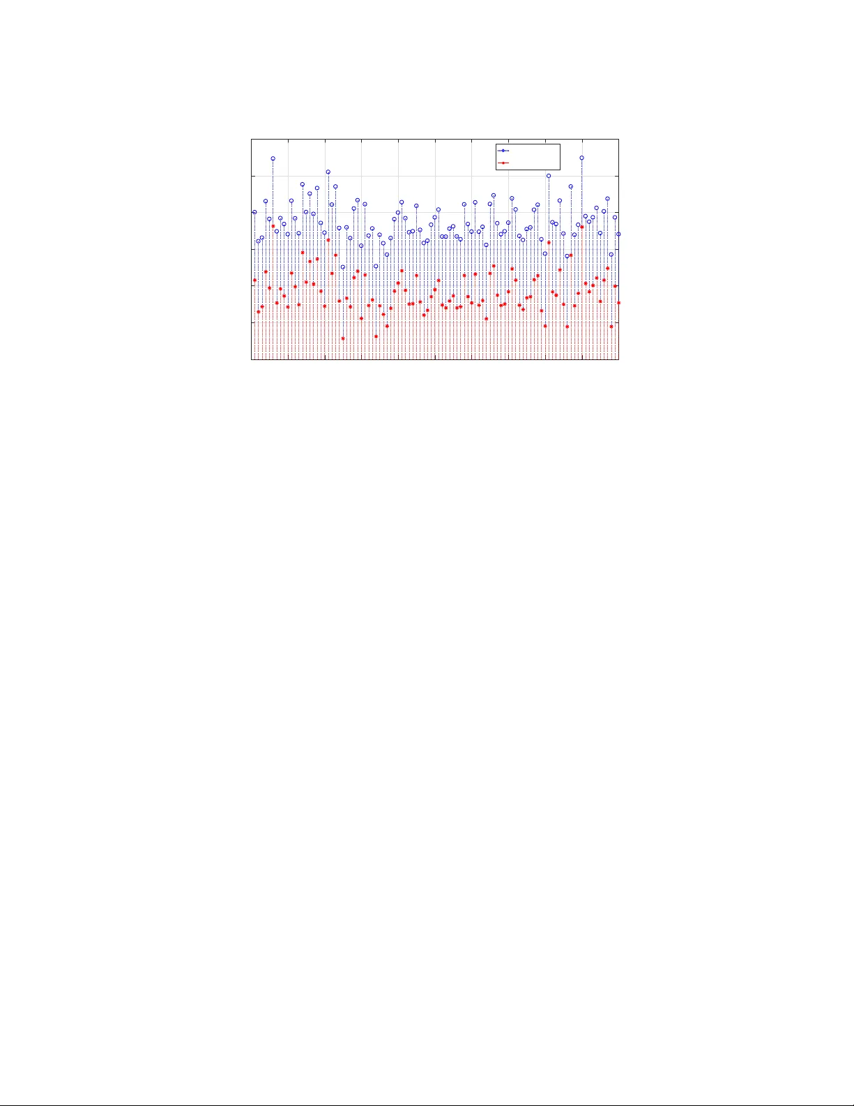
Adaptiv e MPC under Time V arying Uncertain t y: Robust and Sto c hastic Monimo y Bujarbaruah, Xiao jing Zhang, Marko T anask ovic, and F rancesco Borrelli ∗ April 13, 2021 Abstract This pap er deals with the problem of formulating an adaptive Mo del Predictiv e Con trol strategy for constrained uncertain systems. W e consider a linear system, in presence of b ounded time v arying additiv e uncertain ty . The uncertain ty is decoupled as the sum of a pro cess noise with kno wn b ounds, and a time v arying offset that w e wish to identify . The time v arying offset uncertain ty is assumed unkno wn p oint-wise in time. Its domain, called the F easible Parameter Set, and its maximum rate of change are known to the control designer. As new data b ecomes av ailable, w e refine the F easible P arameter Set with a Set Mem b ership Metho d based approac h, using the kno wn b ounds on process noise. W e consider t wo separate cases of robust and probabilistic constrain ts on system states, with hard constraints on actuator inputs. In both cases, we r obustly satisfy the imp osed constrain ts for all p ossible v alues of the offset uncertaint y in the F easible P arameter Set. By imp osing adequate terminal conditions, w e prov e recursiv e feasibilit y and stability of the prop osed algorithms. The efficacy of the prop osed robust and sto chastic Adaptive MPC algorithms is illustrated with detailed n umerical examples. 1 In tro duction Mo del Predictiv e Control (MPC) is an established con trol metho dology for dealing with constrained, and p ossibly uncertain systems [1]–[3]. Primary challenges in MPC design include presence of distur- bances and/or unknown mo del parameters. Disturbances can b e handled by means of robust or c hance constrain ts, and such metho ds are generally well understo o d [4]–[11]. In this pap er, we are lo oking into metho ds for addressing the challenge p osed by mo del uncertainties when adaptation is introduced in the design. If the actual mo del of a system is unknown, adaptive con trol strategies ha ve b een applied for meeting con trol ob jectives and ensuring a system’s stability . Adaptiv e control for unconstrained systems has b een widely studied and is generally well-understoo d [12], [13]. In recen t times, this concept of online mo del adaptation has b een extended to MPC con troller design for systems sub ject to b oth robust and probabilistic constraints [14]–[31]. The v ast ma jorit y of literature on adaptive MPC for uncertain systems has focused on robust constrain t satisfaction. F or linear systems, w orks such as [17], [30], [31] hav e typically focused on impro ving p erformance with the adapted mo dels (e.g. lo w closed-lo op cost), while the constrain ts are ∗ M. Bujarbaruah, X. Zhang and F. Borrelli are with the Department of Mechanical Engineering, Universit y of California Berk eley , Berkeley , CA 94720 USA; e-mail: { monimo yb, xiao jing.zhang, fb orrelli } @b erkeley .edu. M. T anasko vic is with Univ erzitet Singidun um, Belgrade, Serbia; e-mail: mtanask ovic@singudun um.ac.rs. satisfied robustly for all p ossible mo deling errors and all disturbances realizations. Here, the domain (supp ort) of the mo del uncertaint y is not adapted in real-time, whic h ma y lead to sub optimal controllers. The work of [21], [28], [32] deal with b oth time inv ariant and time v arying system uncertaint y in Finite Impulse Response (FIR) domain and pro ve recursiv e feasibilit y and stability [3, Chapter 12] of the prop osed approac hes. Ho wev er, such FIR parametrization restricts application to primarily slow and stable systems. In [25], [33], [34], Linear P arameter V arying (LPV) models are considered, and recursiv e feasibilit y of robust constraints and closed-lo op stabilit y prop erties are ensured in presence of unkno wn, but time-invariant parameters only . The authors in [14] also formulate an adaptiv e MPC strategy for an LPV system using the concept of c omp arison mo dels , but do not consider any disturbances or pro cess noise. F or nonlinear systems, w orks suc h as [15], [16], [19] prop ose robust adaptiv e MPC algorithms, but since these require construction of inv arian t sets [3, Chapter 10] for such systems, they are computationally demanding. Literature on adaptiv e MPC for systems with pr ob abilistic constraints is more limited. The w ork in [23], [24] use data driven approaches for real-time mo del learning together with a sto c hastic MPC con troller, but without guarantees on feasibility and stability . In [27], [29] recursively feasible adaptive sto c hastic MPC algorithms are presen ted, but for static input-output system mo dels only . T o the b est of our knowledge, no adaptive MPC framew ork has b een presented in literature that ensures recursive feasibilit y and stability for systems in state-space under probabilistic constraints. In this pap er, we build on the work of [21], [28], [29], and propose a unified and tractable A daptive MPC framework for systems represen ted by state-space models, that can take in to account both robust and probabilistic state constrain ts, and hard input constrain ts, while guaranteeing recursive feasibilit y and stability . Sp ecifically , w e consider linear systems that are sub ject to b ounded additiv e uncertaint y , whic h is comp osed of: ( i ) a pro cess noise, and ( ii ) an unkno wn, but b ounded offset that w e try to estimate. Given an initial estimate of the offset’s domain, w e iteratively refine it using a Set Membership Metho d based approach [21], as new data b ecomes av ailable. In order to design an MPC controller with the unknown offset, we make sure the constraints on states and inputs are satisfied for all feasible offsets at a time instant. Here a “feasible offset” is an offset b elonging to the current estimation of the offset’s domain. As the feasible offset domain is up dated with data progressively , we obtain an on-line adaptation in the MPC algorithm. F urthermore, the offset uncertaint y present in the system is considered time v arying and its maxim um rate of c hange is assumed b ounded and kno wn [19], [28]. The main con tributions of this pap er can b e summarized as follo ws: • W e prop ose a Set Membership Metho d based mo del adaptation algorithm to estimate and up- date the time v arying offset uncertaint y , using a so-called F easible Parameter Set. The mo del adaptation algorithm guarantees containmen t of the true offset uncertaint y in the F easible Pa- rameter Set at all times. This extends the works of [21], [25], [28], [32], [35] to time v arying mo del uncertain ties in state space. • W e prop ose an adaptive MPC framew ork for systems p erturb ed by such additiv e time v arying offset uncertaint y and pro cess noise. The framework handles robust and c hance constraints on system states resp ectively , with hard input constraints, while using data to progressively obtain offset uncertain ty adaptation. With appropriately chosen terminal conditions, we guarantee re- cursiv e feasibility and Input to State Stabilit y (ISS) of the prop osed adaptive MPC algorithms, whic h is an addition to the work of [23], [24], [31], [36]. Compared to [15], [16], [19], computation of terminal inv ariant sets is simpler, as we fo cus on linear systems. Moreo ver, as opp osed to [17], [30], [31], w e utilize the mo del adaptation information in real-time for mo difying constrain ts. The pap er is organized as follows: in Section 2 we formulate the optimization problems to b e solv ed and also define the imp osed constrain ts. The offset uncertain t y adaptation framework is presented in Section 3. W e propose the Adaptive Robust MPC algorithm in Section 4 and Adaptive Sto chastic MPC algorithm in Section 5. The feasibility and stability prop erties of the aforementioned algorithms are discussed in Section 6. W e then present detailed numerical simulations in Section 7. 2 Problem F ormulation Giv en an initial state x S , we consider uncertain linear time-in v ariant systems of the form: x t +1 = Ax t + B u t + E θ a t + w t , x 0 = x S , (1) where x t ∈ R n is the state at time step t , u t ∈ R m is the input, and A and B are known system matrices of appropriate dimensions. At eac h time step t , the system is affecte d by an i.i.d. random pro cess noise w t ∈ W ⊂ R n , whose probabilit y distribution function (PDF) is assumed known, or can b e estimated empirically from data [37], [38]. F or simplicit y , W is assumed to b e a hyperrectangle containing zero as: W = { w : − ¯ w ≤ w ≤ ¯ w } . (2) W e also consider the presence of θ a t ∈ R p , a b ounded, time v arying offset uncertaint y , which enters the system through the constant known matrix E ∈ R n × p . Remark 1. In r e ality, the additive unc ertainty in the system c ould b e difficult to split into two p arts as c onsider e d in (1) . However, such a de c omp osition enables us to de al with p ar ametric mo del unc er- tainties. A lthough, we have formulate d the pr oblem with only additive unc ertainty in (1) , wher e A and B ar e known matric es, one c an also upp er b ound effe ct of p ar ametric unc ertainties in A and B with an additive unc ertain term (similar to offset E θ a t ) and pr op agate the system dynamics (1) with a chosen set of nominal ¯ A, ¯ B matric es. Assumption 1. We assume the true offset θ a t to b e time varying. The b ounds on the r ate of change of this offset ar e known and given by θ a t − θ a t − 1 = ∆ θ a t ∈ P , for al l t ≥ 0 , wher e the set P = { ∆ θ a ∈ R p : K θ ∆ θ a ≤ l θ , K θ ∈ R r θ × p , l θ ∈ R r θ } . (3) Assumption 2. We also assume that the true offset θ a t lies within a known and nonempty p olytop e Ω at al l times, which c ontains zer o in its interior. That is, θ a t ∈ Ω , ∀ t ≥ 0 , wher e, Ω = { θ : H θ 0 θ ≤ h θ 0 } , (4) for matric es H θ 0 ∈ R r 0 × p and h θ 0 ∈ R r 0 . 2.1 Constrain ts In this pap er w e study tw o different cases of constraint satisfaction, namely ( i ) robust constrain t on states and hard constraints on inputs, and ( ii ) chance constraints on states and hard constraints on inputs. W e define C ∈ R s × n , G ∈ R s × n , D ∈ R s × m , b ∈ R s , h ∈ R s , H u ∈ R o × m and h u ∈ R o . W e can then write the constraints ∀ t ≥ 0 as: Z 1 := { ( x, u ) : C x + D u ≤ b } , (5a) Z 2 := { ( x, u ) : P ( Gx ≤ h ) ≥ 1 − α, H u u ≤ h u } , (5b) where α ∈ (0 , 1) is the admissible probabilit y of constraint violation. W e assume the ab ov e state and input constrain t sets are compact and they con tain the origin. This assumption is key for the stability pro of in Section 6. 2.2 Infinite Horizon Optimization Problems Our goal is to design con trollers that solv e tw o infinite horizon optimal con trol problems, one with constrain ts Z 1 and the other one with Z 2 . They are defined as follows: min u 0 ,u 1 ( · ) ,... X t ≥ 0 ` ( ¯ x t , ¯ u t ) s.t. x t +1 = Ax t + B u t + E θ a t + w t , ¯ x t +1 = A ¯ x t + B ¯ u t + E θ a t , C x t + D u t ≤ b, ∀ w t ∈ W , x 0 = x S , ¯ x 0 = x S , t = 0 , 1 , . . . , (P1) and min u 0 ,u 1 ( · ) ,... X t ≥ 0 ` ( ¯ x t , ¯ u t ) s.t. x t +1 = Ax t + B u t + E θ a t + w t , ¯ x t +1 = A ¯ x t + B ¯ u t + E θ a t , P ( Gx t ≤ h ) ≥ 1 − α, H u u t ≤ h u , x 0 = x S , ¯ x 0 = x S , t = 0 , 1 , . . . , (P2) where θ a t is the time v arying offset present in the system, ¯ x t is the disturbance-free nominal state and ¯ u t = u t ( ¯ x t ) ∈ R m denotes the corresp onding nominal input. The nominal state is utilized to obtain the nominal cost, whic h is minimized in optimization problems (P1) and (P2). W e p oin t out that, as system (1) is uncertain, the optimal con trol problems (P1) and (P2) consist of finding input p olicies [ u 0 , u 1 ( · ) , u 2 ( · ) , . . . ], where u t : R n 3 x t 7→ u t = u t ( x t ) ∈ R m are feedback p olicies. W e approximate solutions to optimization problems (P1) and (P2) by solving corresp onding finite time constrained optimal control problems in a receding horizon fashion. In this pap er, we assume that the offset θ a t in (P1) and (P2) is not known exactly . Therefore, we prop ose a parameter estimation framework to refine our knowledge of θ a t as more data is collected, thus in tro ducing adaptation . 3 Uncertain t y Adaptation The domain of feasible offset θ a t is denoted b y Θ t at time step t , and is called the F e asible Par ameter Set [21]. The goal is to ensure that constrain ts (5a) and (5b) are satisfied for all θ t ∈ Θ t . This guaran tees constrain t satisfaction in presence of the true unknown offset θ a t ∈ Θ t . Our initial estimate for Θ 0 is Ω from Assumption 2, i.e., Θ 0 = Ω. The F easible Parameter Set is then adapted at ev ery time-step as new measuremen ts are a v ailable, utilizing Assumption 1 and Assumption 2. Based on only the measuremen ts at time step t , we denote the p otential domain of the feasible offset at time step t , S t t as: S t t = { θ t ∈ R p : − ¯ w + ¯ ν ≤ − x t + Ax t − 1 + B u t − 1 + E θ t ≤ ¯ w + ¯ ν } , where b ounds ¯ w are given by (2), and from (3), we apply: ¯ ν = min ν { E ν : K θ ν ≤ l θ } , ¯ ν = max ν { E ν : K θ ν ≤ l θ } . (6) No w, for any q ≤ t , the feasible set of offsets for time step t , based on information un til time step q , is obtained as: S q t = { θ t ∈ R p : − ¯ w + ( t − q + 1) ¯ ν ≤ − x q + Ax q − 1 + B u q − 1 + E θ t ≤ ¯ w + ( t − q + 1) ¯ ν } , Using all the ab ov e information un til time step t , we obtain the F easible Parameter Set at time step t , as: Θ t = Ω ∩  \ q =1 , 2 ,...,t S q t  . The ab ov e F easible P arameter Set at time step t can b e written as: Θ t = { θ t ∈ R p : H θ t θ t ≤ h θ t } , (7) where H θ t ∈ R r t × p and h θ t ∈ R r t , r t = r 0 + 2 t is the num b er of facets in the F easible Parameter Set p olytop e Θ t at any given t . As new data is obtained at the next time step ( t + 1), it can b e prov en that [28]: H θ t +1 = [( H θ t ) > , − E > , + E > ] > ∈ R r t +1 × p , h θ t +1 =   h θ t + ∆ h θ t − x t +1 + Ax t + B u t + ¯ w − ¯ ν x t +1 − Ax t − B u t + ¯ w + ¯ ν   ∈ R r t +1 , ∆ h θ t =  0 > r 0 , − ¯ ν > , ¯ ν > , . . . , − ¯ ν > , ¯ ν >  > ∈ R r t . (8) Prop osition 1. Assume that (2) and Assumption 1 hold. Then the F e asible Par ameter Set obtaine d using (7) – (8) is nonempty and c ontains the true offset at al l times, i.e, Θ t 6 = ∅ and θ a t ∈ Θ t for al l t ≥ 0 . Pr o of. See App endix. 4 Adaptiv e Robust MPC In this section we present formulation of the Adaptive Robust MPC algorithm. W e appro ximate the solutions to the infinite horizon optimal control problem (P1) b y solving a finite horizon problem in a receding horizon fashion. 4.1 Robust MPC Problem The MPC controller has to solve the following finite horizon robust optimal con trol problem at each time step: min U t ( · ) t + N − 1 X k = t ` ( ¯ x k | t , ¯ u k | t ) + Q ( ¯ x t + N | t ) s.t. x k +1 | t = Ax k | t + B u k | t + E θ k | t + w k | t , ¯ x k +1 | t = A ¯ x k | t + B ¯ u k | t + E ¯ θ t , C x k | t + D u k | t ≤ b, x t + N | t ∈ X R N , ∀ θ k | t ∈ Θ k | t , ∀ w k | t ∈ W , ∀ k = { t, . . . , t + N − 1 } , x t | t = x t , ¯ x t | t = x t , ¯ θ t ∈ Ω , (9) where x t is the measured state at time step t , x k | t is the prediction of state at time step k , obtained by applying predicted input p olicies [ u t | t , . . . , u k − 1 | t ] to system (1), and { ¯ x k | t , ¯ u k | t } with ¯ u k | t = u k | t ( ¯ x k | t ) denote the disturbance-free nominal state and corresp onding input resp ectively . W e use a nominal p oint estimate of offset, ¯ θ t ∈ Ω to propagate the nominal tra jectory . The predicted F easible P arameter Sets Θ k | t are elab orated in the following section. Notice, the ab ov e minimizes the nominal cost, comprising of p ositiv e definite stage cost ` ( · , · ) and terminal cost Q ( · ) functions. The terminal constraint X R N and terminal cost Q ( · ) are introduced to ensure feasibility and stability prop erties of the MPC controller [1], [3], as we highlight in Section 6. Remark 2. One may design p oint estimates ¯ θ t of the offset for p erformanc e impr ovement, i.e, lower c ost in (9) . F ol lowing [33], one option is to c onstruct the nominal offset estimate ¯ θ t r e cursively with L e ast Me an Squar e filter as ˜ θ t = ¯ θ t − 1 + µE > ( x t − ¯ x t | t − 1 ) , (10a) ¯ θ t = Pro j Ω ( ˜ θ t ) , (10b) wher e Pro j( · ) denotes the Euclide an pr oje ction op er ator, and sc alar µ ∈ R c an b e chosen such that 1 µ > k E k 2 . Prop osition 2. If sup t ≥ 0 k x t k < ∞ and sup t ≥ 0 k u t k < ∞ , then ¯ θ t ∈ Ω and sup ˜ m ∈ N ,w t ∈ W , ¯ θ 0 ∈ Ω ˜ m P t =0 k ˜ x t +1 | t k 2 1 µ k ¯ θ 0 − θ a 0 k 2 + ˜ m P t =0 k w t k 2 ≤ 1 , (11) wher e ˜ x t +1 | t = Ax t + B u t − ¯ x t +1 | t is the one step pr e diction err or, ignoring the effe ct of w t in close d-lo op. Pr o of. See App endix. With b ound (11) on pr e diction err or, finite gain ` 2 stability of the r esulting MPC algorithm c an b e trivial ly pr oven by fol lowing [33, The or em 14], [39, The or em 3.2]. However, sinc e we only fo cus on the r obust c onstr aint satisfaction asp e ct of (9) , we wil l use the nominal offset estimate ¯ θ t = 0 p × 1 for al l t ≥ 0 in the subse quent se ctions. 4.2 Predicted F easible Parameter Sets These Pr e dicte d F e asible Par ameter Sets are constructed along an MPC horizon at time step t , when the measurement at next time step ( t + 1) is yet to b e a v ailable. Definition 1. (Pr e dicte d F e asible Par ameter Sets) The Predicted F easible Parameter Sets at any time step t , ar e the pr e dicte d fe asible domains of the true offset θ a over a pr e diction horizon of length N , b ase d on the information until time step t . These sets ar e denote d as Θ k | t = { θ ∈ R p : H θ k | t θ ≤ h θ k | t } for al l k ∈ { t, t + 1 , . . . , t + N − 2 } , wher e H θ k +1 | t = H θ k | t ∈ R r t × p , (12a) h θ k +1 | t = h θ k | t +  0 > r 0 , − ¯ ν > , ¯ ν > , .., − ¯ ν > , ¯ ν >  > , (12b) with the terminal c ondition, Θ t + N | t = Ω , (13) wher e Ω is define d in Assumption 2. In principle, the Predicted F easible Parameter Sets in (12) are formed after measuring x t at any time step t , and expanding the obtained (from (7)) F easible Parameter Set Θ t o ver the entire horizon of length N , incorp orating parameter rate b ounds (3). Prop osition 3. The Pr e dicte d F e asible Par ameter Sets satisfy the pr op erty Θ k | t +1 ⊆ Θ k | t , for al l k ∈ { t + 1 , t + 2 , . . . , t + N } . Pr o of. See App endix. 4.3 Con trol P olicy Note that optimizing o ver p olicies U ( · ) in (9) is an intractable problem, as it in volv es searching ov er an infinite dimensional function space. Therefore, we restrict ourselv es to the affine disturbance feedbac k parametrization [8], [40] for con trol syn thesis. F or all k ∈ { t, . . . , t + N − 1 } ov er the MPC horizon (of length N ), the control p olicy is given as: u k | t ( x k | t ) : u k | t = k − 1 X j = t M k,j | t ( w j | t + E θ j | t ) + v k | t , (14) where M k | t are the planne d feedbac k gains at time step t and v k | t are the auxiliary inputs. Let us define w t = [ w > t | t , . . . , w > t + N − 1 | t ] > ∈ R nN , θ θ θ t = [ θ > t | t , . . . , θ > t + N − 1 | t ] > ∈ R pN and E = diag( E , E , . . . , E ) ∈ R nN × pN . Then the sequence of predicted inputs from (14) can be stac ked together and compactly written as u t = M t ( w t + E θ θ θ t ) + v t at any time step t , where M t ∈ R mN × nN and v t ∈ R mN are: M t =      0 · · · · · · 0 M t +1 ,t 0 · · · 0 . . . . . . . . . . . . M t + N − 1 ,t · · · M t + N − 1 ,t + N − 2 0      , v t = [ v > t | t , · · · , · · · , v > t + N − 1 | t ] > . 4.4 T ractable Reform ulation Using Section 4.2 and Section 4.3, w e solv e the follo wing tractable reform ulation of robust MPC problem (9): J ? R ( t, x t ) := min M t , v t t + N − 1 X k = t ` ( ¯ x k | t , v k | t ) + Q ( ¯ x t + N | t ) s.t. x k +1 | t = Ax k | t + B u k | t + E θ k | t + w k | t , ¯ x k +1 | t = A ¯ x k | t + B v k | t , u k | t = k − 1 X j = t M k,j | t ( w j | t + E θ j | t ) + v k | t , C x k | t + D u k | t ≤ b, x t + N | t ∈ X R N , ∀ θ k | t ∈ Θ k | t , ∀ w k | t ∈ W , ∀ k = { t, . . . , t + N − 1 } , x t | t = x t , ¯ x t | t = x t . (15) W e use state feedbac k to construct terminal set X R N = { x ∈ R n : Y R x ≤ z R , Y R ∈ R r R × n , z R ∈ R r R } , whic h is the maximal robust p ositive in v ariant set [41] obtained with a state feedbac k controller u = K x , dynamics (1) and constraints (5a). This set has the properties: X R N ⊆ { x | ( x, K x ) ∈ Z 1 } , ( A + B K ) x + w + E θ ∈ X R N , ∀ x ∈ X R N , ∀ w ∈ W , ∀ θ ∈ Ω . (16) Fixed p oint iteration algorithms to numerically compute (16) can b e found in [3], [39]. Notice that (15) is a time varying conv ex optimization problem with ∞− n umber of constraints. An efficien t wa y to reformulate (15) is shown in the App endix. After solving (15), in closed-lo op, w e apply , u t ( x t ) = u ? t | t = v ? t | t (17) to system (1). W e then resolve the problem again at the next ( t + 1)-th time step, yielding a receding horizon strategy . Algorithm 1 Adaptive Robust MPC 1: Set t = 0; initialize F easible Parameter Set Θ 0 = Ω; 2: Compute the parameter rate of change b ounds ¯ ν and ¯ ν from (6); 3: F orm Predicted F easible P arameter Sets Θ k | t for k = { t, . . . , t + N } using (12) and (13); 4: Compute v ? t | t from (15) and apply u t = v ? t | t to (1); 5: Obtain x t +1 , and up date Θ t +1 as given in (8); 6: Set t = t + 1, and return to step 3. 5 Adaptiv e Sto chastic MPC In this section w e presen t the form ulation of the Adaptiv e Sto chastic MPC algorithm. Similar as b efore, we approximate (P2) by solving a finite horizon problem in receding horizon fashion. F or parametrization of con trol p olicies, w e use the same affine disturbance p olicy as in Section 4.3. 5.1 MPC Problem W e use Bonferroni’s inequality [42] to appro ximate the joint chance constraints on states (5b), giv en as: P ( g > j x t ≤ h j ) ≥ 1 − α j , H u u t ≤ h u , ∀ j ∈ { 1 , . . . , s } , (18) where α j ∈ (0 , 1), s P j =1 α j = α and g > j denotes the j -th row of matrix G for all j ∈ { 1 , . . . , s } . T o ensure satisfaction of state constraints in (18), it is sufficient to ensure [43]: P ( g > j x t +1 ≤ h j | x t ) ≥ 1 − α j , j ∈ { 1 , . . . , s } , ∀ t ≥ 0 . (19) Therefore, the sto chastic MPC controller has to solve the following optimal control problem at each time step: min M t , v t t + N − 1 X k = t ` ( ¯ x k | t , v k | t ) + Q ( ¯ x t + N | t ) s.t. x k +1 | t = Ax k | t + B u k | t + E θ k | t + w k | t , ¯ x k +1 | t = A ¯ x k | t + B v k | t , P ( g > j x k +1 | t ≤ h j | x k | t ) ≥ 1 − α j , u k | t = k − 1 X j = t M k,j | t ( w j | t + E θ j | t ) + v k | t , H u u k | t ≤ h u , x t + N | t ∈ X S N , ∀ [ θ t | t , . . . , θ k | t ] ∈ Θ t | t × . . . × Θ k | t , ∀ [ w t | t , . . . , w k − 1 | t ] ∈ W k − t , ∀ k = { t, . . . , t + N − 1 } , ∀ j ∈ { 1 , . . . , s } , x t | t = x t , ¯ x t | t = x t , (20) where the terminal constraint X S N and the terminal cost function Q ( · ) are in tro duced to ensure feasibility and stability prop erties of the MPC controller [1], [3]. 5.2 Chance Constrain t Reformulation The chance constraints in (20) can b e reform ulated as g > j ( Ax k | t + B u k | t + E θ k | t ) ≤ h j − F − 1 g > j w (1 − α j ) , ∀ [ θ t | t , . . . , θ k | t ] ∈ Θ t | t × . . . × Θ k | t , ∀ [ w t | t , . . . , w k − 1 | t ] ∈ W k − t , ∀ j ∈ { 1 , . . . , s } , ∀ k ∈ { t, . . . , t + N − 1 } , (21) where F − 1 g > j w ( · ) is the left quan tile function of g > j w . F rom (1) and (14), using w t = [ w > t | t , . . . , w > t + N − 1 | t ] > ∈ R nN , θ θ θ t = [ θ > t | t , . . . , θ > t + N − 1 | t ] > ∈ R pN , E = diag( E , E , . . . , E ) ∈ R nN × pN and M t ∈ R mN × nN from Section 4.3, we can write, x k | t = A k − t x t | t + B k ( v t + M t w t + M t E θ θ θ t ) + C k ( w t + E θ θ θ t ), where B k = [ A k − t − 1 B , . . . , B , 0 n × m , . . . , 0 n × m ] ∈ R n × mN and C k = [ A k − t − 1 , . . . , I n × n , 0 n × n , . . . , 0 n × n ] ∈ R n × nN [43]. Using this to rewrite LHS of (21), w e obtain: g > j ( Ax k | t + B u k | t + E θ k | t ) = g > j ( A k +1 − t x t + B k +1 v t ) + g > j ( B k +1 M t + A C k )( w t + E θ θ θ t ) + g > j ( E θ k | t ) . (22) Denoting, Γ ? k | t ( M t ) = max w t , θ θ θ t g > j ( B k +1 M t + A C k )( w t + E θ θ θ t ) + g > j ( E θ k | t ), and with (22), w e rewrite (21) as g > j ( A k +1 − t x t + B k +1 v t ) ≤ h j − Γ ? k | t ( M t ) − F − 1 g > j w (1 − α j ) , ∀ θ k | t ∈ Θ k | t , ∀ j ∈ { 1 , . . . , s } , ∀ k ∈ { t, . . . , t + N − 1 } . A t any given t , the chance constraints (21) are th us robustly satisfied for all offsets [ θ t | t , . . . , θ k | t ] ∈ Θ t | t × . . . × Θ k | t and [ w t | t , . . . , w k − 1 | t ] ∈ W k − t for all k ∈ { t, . . . , t + N − 1 } . 5.3 T ractable MPC Problem Using the previous results, (20) is equiv alen t to the follo wing deterministic optimization problem: J ? S ( t, x t ) := min M t , v t t + N − 1 X k = t ` ( ¯ x k | t , v k | t ) + Q ( ¯ x t + N | t ) s.t. x k +1 | t = Ax k | t + B u k | t + E θ k | t + w k | t , ¯ x k +1 | t = A ¯ x k | t + B v k | t , g > j ( A k +1 − t x t | t + B k +1 v t ) ≤ h j − Γ ? k | t ( M t ) − F − 1 g > j w (1 − α j ) , u k | t = k − 1 X j = t M k,j | t ( w j | t + E θ j | t ) + v k | t , H u u k | t ≤ h u , x t + N | t ∈ X S N , ∀ θ k | t ∈ Θ k | t , ∀ k = { t, . . . , t + N − 1 } , ∀ j ∈ { 1 , . . . , s } , x t | t = x t , ¯ x t | t = x t , (23) where the terminal set X S N = { x ∈ R n : Y S x ≤ z S , Y S ∈ R r S × n , z S ∈ R r S } has the prop erties: ( A + B K ) x + E θ + w ∈ X S N , H u ( K x ) ≤ h u , g > j ( A + B K ) x ≤ − g > j ( E θ ) + h j − F − 1 g > j w (1 − α j ) , ∀ j ∈ { 1 , . . . , s } , ∀ θ ∈ Ω , ∀ w ∈ W , ∀ x ∈ X S N . (24) Notice that (23) is a time varying conv ex optimization problem. An efficient w ay to reform ulate (23) is shown in the App endix. After solving (23), in closed-lo op, w e apply the first input, u t ( x t ) = u ? t | t = v ? t | t (25) to system (1). W e then resolve the problem again at the next ( t + 1)-th time step, yielding a receding horizon control design. Algorithm 2 Adaptive Sto chastic MPC 1: Set t = 0; initialize F easible Parameter Set Θ 0 = Ω; 2: Compute the parameter rate of change b ounds ¯ ν and ¯ ν from (6); 3: F orm Predicted F easible P arameter Sets Θ k | t for k = { t, . . . , t + N } using (12) and (13); 4: Compute v ? t | t from (23) and apply u t = v ? t | t to (1); 5: Obtain x t +1 , and up date Θ t +1 as given in (8); 6: Set t = t + 1, and return to step 3. 6 F easibilit y and Stabilit y Guaran tees In this section we discuss feasibilit y and stability prop erties of Algorithm 1 and Algorithm 2. Assumption 3. The stage c ost ` ( · , · ) in (15) and (23) is chosen as ` ( ¯ x k | t , v k | t ) = ¯ x > k | t P ¯ x k | t + v > k | t Rv k | t for some P = P >  0 and R = R >  0 , which is c ontinuous and p ositive definite. Assumption 4. The terminal c ost Q ( · ) in (15) (or (23) ) is chosen as a Lyapunov function in the terminal set X R N (or X S N ) for the nominal close d-lo op system x + = ( A + B K ) x , for al l ¯ x ∈ X R N (or X S N ). That is, Q (( A + B K ) x ) − Q ( x ) ≤ − x > ( P + K > RK ) x . 6.1 F easibilit y Theorem 1. L et Assumptions 1-2 hold and c onsider the r obust optimization pr oblem (15) . L et this optimization pr oblem b e fe asible at time step t = 0 with Θ 0 = Ω with Ω define d in Assumption 2. Assume the F e asible Par ameter Set Θ t in (15) is adapte d b ase d on (7) - (8) . Then, (15) r emains fe asible at al l time steps t ≥ 0 , if the state x t is obtaine d by applying the close d-lo op MPC c ontr ol law (15) - (17) to system (1) . Pr o of. Let the optimization problem (15) b e feasible at time step t . Let us denote the corresp onding optimal input p olicies as [ u ? t | t , u ? t +1 | t ( · ) , . . . , u ? t + N − 1 | t ( · )]. Assume the MPC controller u ? t | t is applied to (1) in closed-lo op and Θ t +1 is up dated according to (8). Consider a candidate p olicy sequence at the next time step as: U t +1 ( · ) = [ u ? t +1 | t ( · ) , . . . , u ? t + N − 1 | t ( · ) , K x t + N | t +1 ] . (26) W e observe the follo wing t wo facts: ( i ) from Prop osition 2, Θ k | t +1 ⊆ Θ k | t , for all k ∈ { t + 1 , t + 2 , . . . , t + N } , and ( ii ) from (16), terminal set X R N is robust p ositiv e inv ariant for all w ∈ W , and for all θ ∈ Ω, with state feedback controller K x . Using ( i ) w e conclude [ u ? t +1 | t ( · ) , u ? t +2 | t ( · ) , . . . , u ? t + N − 1 | t ( · )] is an ( N − 1) step feasible sequence at ( t + 1) (excluding terminal condition), since at previous time step t , it robustly satisfied all stage constraints in (15) for Θ k | t , for all k ∈ { t + 1 , t + 2 , . . . , t + N − 1 } . With this feasible sequence, x t + N | t +1 ∈ X R N . Using ( ii ) we conclude, app ending the ( N − 1) step feasible sequence with K x t + N | t +1 ensures x t + N +1 | t +1 ∈ X R N , satisfying the terminal constrain t at ( t + 1). 6.2 Input to State Stabilit y W e denote the N -step robust controllable set [3, Chapter 10] to the terminal set X R N under the MPC p olicy (17) by X R 0 , which is compact and con tains the origin. Definition 2. (Input to State Stability [44]): Consider system (1) in close d-lo op with the MPC c on- tr ol ler (17) , obtaine d fr om (7) - (8) - (15) , given by x t +1 = Ax t + B v ? t | t + E θ a t + w t , ∀ t ≥ 0 . (27) The origin is define d as Input to State Stable (ISS), with a r e gion of attr action X R 0 ⊂ R n , if ther e exists K ∞ functions α 1 ( · ) , α 2 ( · ) , α 3 ( · ) , a K function σ ( · ) and a function V ( · , · ) : R × X R 0 7→ R ≥ 0 c ontinuous at the origin such that, α 1 ( k x t k ) ≤ V ( t, x ) ≤ α 2 ( k x t k ) , ∀ x ∈ X R 0 , ∀ t ≥ 0 , V ( t + 1 , x t +1 ) − V ( t, x t ) ≤ − α 3 ( k x t k ) + σ ( k w i + E θ a i k L ∞ ) , wher e k · k denotes the Euclide an norm and signal norm k d i k L ∞ = sup i = { 0 , 1 ,...,t } k d i k . F unction V ( · , · ) is c al le d an ISS Lyapunov function for (27) . Theorem 2. L et Assumptions 1-4 hold. Then, the optimal c ost of (15) , i.e, J ? R ( · , · ) is an ISS Lyapunov function for close d-lo op system (27) . Pr o of. F rom Assumption 3 we kno w that at time step t , α 1 ( k x t k 2 ) ≤ ` ( x t , 0) ≤ J ? R ( t, x t ) for some α 1 ( · ) ∈ K ∞ . Moreov er, since (15) is a parametric QP , J ? R ( t, 0) = 0, and X R 0 is compact, using similar argumen ts as [8, Theorem 23], w e kno w J ? R ( t, x t ) ≤ α 2 ( k x t k 2 ) for som e α 2 ( · ) ∈ K ∞ . Note that as opp osed to [8], our α 2 ( · ) is not obtained via Lipschitz con tin uity of the v alue function, since in our case, V ( t, x ) is assumed contin uous only at the origin. The existence of α 2 ( · ) is ensured by the compactness of the constrain t sets in (5). No w sa y J ? R ( t, x t ) = t + N − 1 X k = t ` ( ¯ x ? k | t , v ? k | t ) + Q ( ¯ x ? t + N | t ) , = ` ( ¯ x ? t | t , v ? t | t ) + q ( ¯ x ? t +1 | t ) , (28) where [ ¯ x ? t | t , . . . , ¯ x ? t + N | t ] is the optimal predicted nominal tra jectory under the optimal nominal input sequence U ? t ( ¯ x t ) = [ u ? t | t ( ¯ x t | t ) , . . . , u ? t + N − 1 | t ( ¯ x t + N − 1 | t )] applied to nominal dynamics in (15), and q ( ¯ x ? t +1 | t ) pro vides the total cost from ( t + 1) to ( t + N ) under p olicy U ? t ( ¯ x t ). W e prov ed that (26) is a feasible p olicy sequence for (15) at time step ( t + 1), where x t +1 = ¯ x t +1 is obtained with (27). With this feasible sequence, the optimal cost of (15) at ( t + 1) is b ounded as J ? R ( t + 1 , x t +1 ) ≤ t + N − 1 X k = t +1 ` ( ¯ x k | t +1 , v ? k | t ) + Q ( ¯ x t + N | t +1 ) , = q ( ¯ x t +1 | t +1 ) , (29) where w e ha v e used Assumption 4 and the feasible nominal tra jectory ¯ x k | t +1 = A k − t − 1 ( Ax t + B v ? t | t + w t + E θ a t ) + k − 1 P i = t +1 A k − 1 − i B u ? i | t ( ¯ x k | t +1 ), for k = { t + 2 , . . . , t + N } . Moreo ver, w e know that ¯ x t +1 | t +1 = ¯ x ? t +1 | t + w t + E θ a t . (30) Com bining (28)–(30) w e obtain, J ? R ( t + 1 , x t +1 ) − J ? R ( t, x t ) = q ( ¯ x ? t +1 | t + w t + E θ a t ) − ` ( ¯ x ? t | t , v ? t | t ) − q ( ¯ x ? t +1 | t ) , ≤ − ` ( ¯ x ? t | t , v ? t | t ) + L q k w t + E θ a t k , ≤ − ` ( ¯ x ? t | t , 0) + L q k w t + E θ a t k , ≤ − α 3 ( k x t k 2 ) + L q k w i + E θ a i k L ∞ , with α 1 ( · ) = α 3 ( · ) , where q ( · ) is L q -Lipsc hitz, as q ( · ) is a sum of quadratic terms in compact (5a). Hence the origin of (27) is ISS. Remark 3. F e asibility and stability of Algorithm 2 c an b e pr oven in the exact same manner and henc e is omitte d. 7 Numerical Sim ulations W e consider the following infinite horizon optimal con trol problem with unknown offset θ a t that satisfies Assumption 1 and Assumption-2: min u 0 ,u 1 ( · ) ,... X t ≥ 0 k ¯ x t k 2 2 + 10 k ¯ u t k 2 2 s.t. x t +1 = Ax t + B u t ( x t ) + E θ a t + w t , ¯ x t +1 = A ¯ x t + B ¯ u t + E ¯ θ t , P n  − 5 − 2 . 5  ≤ x t ≤  5 2 . 5  o ≥ 1 − α, − 4 ≤ u t ( x t ) ≤ 4 , ∀ w t ∈ W , ∀ θ t ∈ Θ t , x 0 = x S , ¯ x 0 = x S , t = 0 , 1 , . . . , (31) Figure 1: F easible Parameter Set Ev olution where A =  1 . 2 1 . 5 0 1 . 3  and B = [0 , 1] > , and F easible Parameter Set Θ t is up dated based on (7)–(8) for all time steps t ≥ 0. F or the robust MPC controller we pick α = 0 and for the sto chastic MPC α = 0 . 4, which w e split using Bonferroni’s inequality as α 1 = α 2 = α/ 2 for eac h of the t wo individual state constraints. Process noise w t ∈ W = { w ∈ R 2 : || w || ∞ ≤ 0 . 1 } . The initial F easible Parameter Set is defined as Ω = Θ 0 = { θ ∈ R 2 : [ − 0 . 5 , − 0 . 5] > ≤ θ ≤ [0 . 5 , 0 . 5] > } . The true offset parameter θ a t is time v arying, with rate b ounded by the p olytop e P := [ − 0 . 05 , − 0 . 05] > ≤ ∆ θ a t ≤ [0 . 05 , 0 . 05] > . F or n umerical simulations, we generate a true offset that starts from θ a 0 = [0 . 49 , 0 . 49] > , and has a rate of c hange ∆ θ a t = [ − 0 . 0395 , − 0 . 0395] > as sho wn in Fig. 1. The matrix E ∈ R 2 × 2 is pic ked as the identit y matrix. The Adaptive Robust MPC in (15), (17), and the Adaptive Sto chastic MPC in (23), (25) are implemen ted with a control horizon of N = 6, and the feedback gain K in (16) and (24), is chosen to b e the optimal LQR gain for system x + = Ax + B u with parameters Q LQR = I and R LQR = 10. Initial state for b oth algorithms is x S = [ − 3 . 21 , − 0 . 25] > . Fig. 1 sho ws the recursiv e adaptation of the F easible Parameter Set and time ev olution of the true offset θ a t . The true parameter lies within Ω, and is alw ays captured by Θ t at all times. This ev olution is k ept identical for all simulation scenarios with both the algorithms. Fig. 2 shows the Mon te Carlo sim ulations for 100 different sampled tra jectories with Adaptiv e Robust MPC, whic h highligh ts satisfaction of constraints in (31) robustly ( α = 0) for all feasible offset uncertainties θ t ∈ Θ t and pro cess noise w t ∈ W , for all t ≥ 0. Suc h robust satisfaction of constraints is crucial for safety critical applications. On the other hand, Adaptive Sto chastic MPC could b e applied in scenarios which are not safet y critical, and where constraint violations are tolerated to improv e p erformance (for example, low er closed-lo op cost). Fig. 3 shows Mon te Carlo simulations for 100 different sampled tra jectories from Adaptiv e Sto c hastic MPC with the same pro cess noise sequences as used for the previous example. This highlights satisfaction of c hance constraints in (31) for all feasible offset uncertain ties θ t ∈ Θ t for all t ≥ 0. The total empirical constrain t violation probabilit y is appro ximately 18%, whic h is lo wer than 0 5 10 15 20 25 Time [s] -5 0 5 x 1 Constraints 0 5 10 15 20 25 Time [s] -5 0 5 x 2 Constraints Figure 2: Mon te Carlo Sim ulation of Robust Case the allo w ed maxim um v alue of 40%. The closed-lo op costs, ∞ P t =0 ` ( x ? t | t , v ? t | t ), of b oth the algorithms for 0 5 10 15 20 25 Time [s] -5 0 5 x 2 Constraints 0 5 10 15 20 25 Time [s] -5 0 5 x 1 Constraints Figure 3: Mon te Carlo Sim ulation of Sto c hastic Case the ab o ve Monte Carlo Simulations (under identical disturbance ( w t ) realizations, θ a t , initial conditions and MPC horizon lengths for b oth algorithms) are compared in Fig. 4. The Adaptive Sto chastic MPC algorithm deliv ers a reduction of 13% in av erage closed-lo op cost compared to Adaptiv e Robust MPC. This indicates p erformance gain at the exp ense of hard constrain t violations. Additionally , Fig. 5 sho ws the closed-lo op MPC cost at each time step t , ` ( x ? t | t , v ? t | t ), plotted o ver 100 different tra jectories, for the en tire length of simulation duration. It can b e inferred from Fig. 5 that the bulk of the closed-lo op cost reduction due to Adaptive Sto c hastic MPC ov er all simulated tra jectories seen in Fig. 4, occurs near the constraint violation zone (b et ween 2 seconds to 4 seconds). 0 10 20 30 40 50 60 70 80 90 100 Monte Carlo Simulation Count 550 600 650 700 750 800 850 Robust Stochastic Figure 4: Comparison of Closed-Lo op Cost ∞ P t =0 ` ( x ? t | t , v ? t | t ) Ac kno wledgemen t W e ac knowledge Ugo Rosolia for helpful discussions and reviews. This w ork w as partially funded by Office of na v al Researc h Gran t ONR-N00014-18-1-2833. 8 Conclusions In this pap er we prop osed an adaptive MPC framework that handles b oth robust and probabilistic constrain ts. A Set Membership Metho d based approac h is used to learn a b ounded and time v arying offset uncertain ty in the model with av ailable data from the system. W e prov ed recursiv e feasibility and input to state stability of resulting MPC algorithms in presence of b ounded additive disturbance/noise. W e sho w ed the v alidity and efficacy of the prop osed approac hes in detailed n umerical simulations. App endix Pro of of Prop osition 1 W e pro ve Prop osition 1 using induction, following the proof of the same in [28]. A t time step t = 0 we kno w that Θ 0 = Ω and from Assumption 2, Ω is nonempty and θ a 0 ∈ Ω. Now using inductive argumen t, let us assume that the claim holds true for some t ≥ 0. That is, for some nonempty Θ t , w e ha v e θ a t ∈ Θ t . No w we must prov e Θ t +1 6 = φ and θ a t +1 ∈ Θ t +1 . Let us define the following matrices: H θ t = [( H θ 0 ) > , ( ¯ H θ t ) > ] > ∈ R r t × p , h θ t = [( h θ 0 ) > , ( ¯ h θ t ) > ] > ∈ R r t , ∆ h θ t = [( 0 r 0 ) > , (∆ ¯ h θ t ) > ] > ∈ R r t , 0 2 4 6 8 10 12 14 16 18 Time [s] 0 100 200 300 400 500 Robust Stochastic Figure 5: Stage Costs ( ` ( x ? t | t , v ? t | t )) in Closed-Lo op where r t = r 0 + 2 t, ∀ t ≥ 0 is the num b er of faces of the F easible Parameter Set p olytop e Θ t . Now from Assumption 2 w e know: H θ 0 θ a t +1 ≤ h θ 0 , (32) and from inductiv e assumptions w e know that ¯ H θ t θ a t ≤ ¯ h θ t . Therefore, we can ensure the following holds: ¯ H θ t θ a t +1 ≤ ¯ h θ t + ∆ ¯ h θ t . (33) Moreo ver, we kno w that: − E θ a t +1 ≤ − x t +1 + Ax t + B u t + ¯ w − ¯ ν, (34a) + E θ a t +1 ≤ x t +1 − Ax t − B u t + ¯ w + ¯ ν. (34b) Hence, from (32), (33) and (34) w e can ha ve, H θ t +1 θ a t +1 ≤ h θ t +1 , where H θ t +1 = [( H θ 0 ) > , ( ¯ H θ t ) > , − E > , + E > ] > ∈ R r t +1 × p , h θ t +1 =     h θ 0 ¯ h θ t + ∆ ¯ h θ t − x t +1 + Ax t + B u t + ¯ w − ¯ ν x t +1 − Ax t − B u t + ¯ w + ¯ ν     ∈ R r t +1 . This prov es that Θ t +1 is nonempty and con tains the actual offset uncertaint y θ a t +1 at the ( t + 1)-th time step. This concludes the pro of. Pro of of Prop osition 2 Utilizing the con traction prop erty of Euclidean pro jection in (10b) similar to [33], we can write 1 µ k ¯ θ t +1 − θ a t +1 k 2 − 1 µ k ¯ θ t − θ a t k 2 ≤ 1 µ k ˜ θ t +1 − θ a t +1 k 2 − 1 µ k ¯ θ t − θ a t k 2 , where k · k is the Euclidean norm. This gives 1 µ k ¯ θ t +1 − θ a t +1 k 2 − 1 µ k ¯ θ t − θ a t k 2 ≤ 1 µ k ˜ θ t +1 − θ a t k 2 + 2 µ ( ˜ θ t +1 − ¯ θ t ) > ( ¯ θ t − θ a t ) + 2 µ ˜ θ > t +1 ( θ a t − θ a t +1 ) , = 1 µ k µE > ( ˜ x t +1 | t + w t ) k 2 + 2( ˜ x t +1 | t + w t ) > E ( ¯ θ t − θ a t ) + 2 µ ˜ θ > t +1 ( θ a t − θ a t +1 ) , ≤ 1 µ k µE > ( ˜ x t +1 | t + w t ) k 2 + 2( ˜ x t +1 | t + w t ) > E ( ¯ θ t − θ a t ) + 2 µ k ˜ θ t +1 kk ( θ a t − θ a t +1 ) k . Consider Ω and P sets from Assumption 1 and Assumption 2. Define sup ω ∈ Ω k ω k = ω M and sup p ∈P k p k = p M . Then the ab o ve inequality can b e written as 1 µ k ¯ θ t +1 − θ a t +1 k 2 − 1 µ k ¯ θ t − θ a t k 2 ≤ 1 µ k µE > ( ˜ x t +1 | t + w t ) k 2 + 2( ˜ x t +1 | t + w t ) > E ( ¯ θ t − θ a t ) + 2 µ ω M p M , ≤ ( µ k E k 2 − 1) k ˜ x t +1 | t + w t k 2 − k ˜ x t +1 | t k 2 + k w t k 2 + 2 µ ω M p M , ≤ −k ˜ x t +1 | t k 2 + k w t k 2 , since from Remark 2 we know 1 µ > k E k 2 , and we hav e used x t +1 − ¯ x t +1 | t = ˜ x t +1 | t + w t and ˜ x t +1 | t = E ( θ a t − ¯ θ t ). Summing b oth sides of the inequality from 0 to ˜ m leads to a telescopic sum on the LHS, and we obtain, 1 µ k ¯ θ ˜ m +1 − θ a ˜ m +1 k 2 + ˜ m X t =0 k ˜ x t +1 | t k 2 ≤ ˜ m X t =0 k w t k 2 + 1 µ k ¯ θ 0 − θ a 0 k 2 , whic h, up on division by RHS on b oth sides gives sup ˜ m ∈ N ,w t ∈ W , ¯ θ 0 ∈ Ω ˜ m P t =0 k ˜ x t +1 | t k 2 1 µ k ¯ θ 0 − θ a 0 k 2 + m P t =0 k w t k 2 ≤ 1 . Pro of of Prop osition 3 F rom the definition of Θ t +1 | t in (12), w e see that, H θ t +1 = [( H θ t +1 | t ) > , − E > , + E > ] > , h θ t +1 =   h θ t +1 | t − x t +1 + Ax t + B u t + ¯ w − ¯ ν x t +1 − Ax t − B u t + ¯ w + ¯ ν   . So Θ t +1 | t +1 ⊆ Θ t +1 | t . No w, the matrices of the Predicted F easible P arameter Sets at next time step, H θ k | t +1 and h θ k | t +1 for all k ∈ { t + 2 , . . . , t + N − 1 } are formed from H θ t +1 and h θ t +1 b y construction. Therefore, for all k ∈ { t + 2 , . . . , t + N − 1 } , H θ k | t +1 = [( H θ k | t ) > , − E > , + E > ] > , h θ k | t +1 =   h θ k | t − x t +1 + Ax t + B u t + ¯ w − ¯ ν x t +1 − Ax t − B u t + ¯ w + ¯ ν   , where H θ k | t and h θ k | t are given by (12). So, for all k ∈ { t + 2 , . . . , t + N − 1 } , each of the sets for Θ k | t +1 are formed by the same inequalities whic h form Θ k | t , app ended by tw o extra ro ws from the new measuremen t. Therefore, Θ k | t +1 ⊆ Θ k | t for all k ∈ { t + 2 , . . . , t + N − 1 } . Moreo ver, from (13), Θ t + N | t = Ω. Using this, H θ t + N | t +1 = [( H θ 0 ) > , − E > , + E > ] > , h θ t + N | t +1 =   h θ 0 − x t +1 + Ax t + B u t + ¯ w − ¯ ν x t +1 − Ax t − B u t + ¯ w + ¯ ν   , and therefore Θ t + N | t +1 ⊆ Θ t + N | t = Ω from the definition of Ω in (4). This prov es the prop osition. Dualization of Robust Problem In this section w e show how the robust MPC problem (15) can b e reform ulated for efficient solving. The constraints in (15) can be compactly written with similar notations as [8]: F R v t + max w t , θ θ θ t ( F R M t + G R )( w t + E θ θ θ t ) ≤ c R + H R x t , (35) where w e denote, v t = [ v > t | t , v > t +1 | t , . . . , v > t + N − 1 | t ] > ∈ R mN , θ θ θ t = [ θ > t | t , . . . , θ > t + N − 1 | t ] > ∈ R pN for all θ k | t ∈ Θ k | t , for all k ∈ { t, . . . , t + N − 1 } , E = diag( E , . . . , E ) ∈ R nN × pN and w t = [ w > t | t , . . . , w > t + N − 1 | t ] > ∈ R nN . The matrices ab ov e in (35) F R ∈ R ( sN + r R ) × mN , G R ∈ R ( sN + r R ) × nN , c R ∈ R sN + r R and H R ∈ R ( sN + r R ) × n are obtained as: F R =        D 0 s × m · · · 0 s × m C B D · · · 0 s × m . . . . . . . . . . . . C A N − 2 B C A N − 3 B · · · D Y R A N − 1 B Y R A N − 2 B · · · Y R B        , G R =        0 s × n 0 s × n · · · 0 s × n C 0 s × n · · · 0 s × n . . . . . . . . . . . . C A N − 2 C A N − 3 · · · 0 s × n Y R A N − 1 Y R A N − 2 · · · Y R        , c R = [ b > , . . . , b > , z > R ] , H R = − [ C > , ( C A ) > , . . . , ( C A N − 1 ) > , ( Y R A N ) > ] > . F or k = { t, . . . , t + N − 1 } , denote the set of polytop es S R k | t = { w ∈ W , θ ∈ Θ k | t : S R k | t ( w + E θ ) ≤ h R k | t } . Then we can define a p olytop e S R = { w t + E θ θ θ t ∈ R nN : S R ( w t + E θ θ θ t ) ≤ h R , S R ∈ R a R × nN , h R ∈ R a R } with, S R = diag( S R t | t , . . . , S R t + N − 1 | t ) , h R = [( h R t | t ) > , . . . , ( h R t + N − 1 | t ) > ] > . No w (35) can b e written with auxiliary decision v ariables Z R ∈ R a R × ( sN + r R ) using duality of linear programs as, F R v t + Z > R h R ≤ c R + H R x t , ( F R M t + G R ) = Z > R S R , Z R ≥ 0 , whic h is a tractable linear programming problem that can b e efficiently solved with any existing solver for real-time implemen tation of Algorithm 1. Dualization of Sto c hastic Problem In this section we show ho w the sto chastic MPC problem (23) can b e reform ulated for efficient solving. The state constrain ts in (23) can be compactly written as: F (1) S v t + max w t , θ θ θ t ( F (2) S ¯ M t + G S )  w t + E θ θ θ t θ θ θ t  ≤ c S + H S x t . (37) where v t , θ θ θ t , E , w t are defined in Section 4.3, and ¯ M t =  M t mN × nN 0 mN × pN 0 pN × nN 0 pN × pN  . The matrices F (1) S ∈ R ( sN + r S ) × mN , F (2) S ∈ R ( sN + r S ) × ( mN + pN ) , G S ∈ R ( sN + r S ) × ( nN + pN ) , c S ∈ R sN + r S and H S ∈ R ( sN + r S ) × n ab o v e in (37), are obtained as: F (1) S =  ( G B t +1 ) > , ( G B t +2 ) > , . . . , ( G B t + N ) > , ( Y S B t + N ) >  > , F (2) S = diag( G, G, . . . , Y S )        B t +1 0 n × p · · · 0 n × p B t +2 0 n × p · · · 0 n × p . . . . . . . . . . . . B t + N 0 n × p · · · 0 n × p B t + N 0 n × p · · · 0 n × p        , G S = diag( G, G, . . . , Y S )        A C t A C t +1 . . . A C t + N − 1 E nN × pN C t + N 0 n × pN        , c S = [ h j − F − 1 g > j w (1 − α j ) , . . . , h j − F − 1 g > j w (1 − α j ) , z > S ] , ∀ j ∈ { 1 , . . . , s } , H S = − [( GA ) > , ( GA 2 ) > , . . . , ( GA N ) > , ( Y S A N ) > ] > . F or k = { t, . . . , t + N − 1 } , denote the set of p olytop es S S k | t = { w ∈ W , θ ∈ Θ k | t : S S k | t  w + E θ θ  ≤ h S k | t } , then w e can define a p olytop e S S = { w t , θ θ θ t ∈ R ( nN + pN ) : S S  w t + E θ θ θ t θ θ θ t  ≤ h S , S S ∈ R a S × ( nN + pN ) , h S ∈ R a S } with, S S = diag( S S t | t , . . . , S S t + N − 1 | t ) , h S = [( h S t | t ) > , . . . , ( h S t + N − 1 | t ) > ] > . Now (37) can b e written with auxiliary decision v ariables Z S ∈ R a S × ( sN + r S ) using duality of linear programs as: F (1) S v t + Z > S h S ≤ c S + H S x t , (38a) ( F (2) S ¯ M t + G S ) = Z > S S S , Z S ≥ 0 . (38b) Moreo ver, (23) imp oses input constraints given by H u u k | t ≤ h u , for all k ∈ { t, . . . , t + N − 1 } , and for all t ≥ 0. This can b e written as: ¯ H u v t + max w t , θ θ θ t ¯ H u ( M t ( w t + E θ θ θ t )) ≤ ¯ h u , (39) where ¯ H u = diag( H u , . . . , H u ) ∈ R oN × mN , ¯ h u = [ h > u , . . . , h > u ] > ∈ R oN . Similar to (38), (39) can b e written with auxiliary decision v ariables Z u ∈ R a R × oN as: ¯ H u v t + Z > u h R ≤ ¯ h u , (40a) ¯ H u M t = Z > u S R , Z u ≥ 0 , (40b) using S R and h R from the previous section. Clearly , (38) and (40) constitute a tractable linear pro- gramming problem that can b e efficiently solved with any existing solver for real-time implementation of the Algorithm 2. References [1] D. Q. Ma yne, J. B. Rawlings, C. V. Rao, and P . O. Scok aert, “Constrained mo del predictiv e con trol: Stability and optimalit y,” Automatic a , v ol. 36, no. 6, pp. 789–814, 2000. [2] M. Morari and J. H. Lee, “Model predictiv e control: Past, present and future,” Computers & Chemic al Engine ering , vol. 23, no. 4, pp. 667–682, 1999. [3] F. Borrelli, A. Bemp orad, and M. Morari, Pr e dictive Contr ol for Line ar and Hybrid Systems . Cam bridge Universit y Press, 2017. [4] M. V. Kothare, V. Balakrishnan, and M. Morari, “Robust constrained mo del predictive con trol using linear matrix inequalities,” A utomatic a , vol. 32, no. 10, pp. 1361–1379, 1996. [5] A. T. Sch w arm and M. Nik olaou, “Chance-constrained model predictiv e con trol,” AIChE Journal , v ol. 45, no. 8, pp. 1743–1752, 1999. [6] J. M. Carson I I I, B. A¸ cıkme ¸ se, R. M. Murray, and D. G. MacMartin, “A robust mo del predictive con trol algorithm augmented with a reactive safety mo de,” Automatic a , v ol. 49, no. 5, pp. 1251– 1260, 2013. [7] W. Langson, I. Chrysso choos, S. Rak o vic, and D. Q. Mayne, “Robust mo del predictive con trol using tub es,” Automatic a , vol. 40, no. 1, pp. 125–133, 2004. [8] P . J. Goulart, E. C. Kerrigan, and J. M. Maciejowski, “Optimization ov er state feedbac k p olicies for robust con trol with constraints,” Automatic a , v ol. 42, no. 4, pp. 523–533, 2006. [9] D Limon, I Alv arado, T Alamo, and E. Camacho, “Robust tub e-based mp c for tracking of con- strained linear systems with additiv e disturbances,” Journal of Pr o c ess Contr ol , vol. 20, no. 3, pp. 248–260, 2010. [10] R. T emp o, G. Calafiore, and F. Dabbene, R andomize d algorithms for analysis and c ontr ol of unc ertain systems: with applic ations . Springer Science & Business Media, 2012. [11] X. Zhang, M. Kamgarp our, A. Georghiou, P . Goulart, and J. Lygeros, “Robust optimal con trol with adjustable uncertain ty sets,” A utomatic a , v ol. 75, pp. 249–259, 2017. [12] S. Sastry and M. Bo dson, A daptive Contr ol: Stability, Conver genc e and R obustness . Courier Cor- p oration, 2011. [13] M. Krstic, I. Kanellak op oulos, and P . V. Kokoto vic, Nonline ar and adaptive c ontr ol design . Wiley, 1995. [14] H. F ukushima, T.-H. Kim, and T. Sugie, “Adaptive mo del predictiv e control for a class of con- strained linear systems based on the comparison mo del,” Au tomatic a , vol. 43, no. 2, pp. 301–308, 2007. [15] D. DeHaan and M. Gua y, “Adaptiv e robust mp c: A minimally-conserv ativ e approac h,” in 2007 A meric an Contr ol Confer enc e , Jul. 2007, pp. 3937–3942. [16] V. Adetola, D. DeHaan, and M. Guay, “Adaptive mo del predictiv e con trol for constrained non- linear systems,” Systems & Contr ol L etters , vol. 58, no. 5, pp. 320–326, 2009. [17] A. Aswani, H. Gonzalez, S. S. Sastry, and C. T omlin, “Prov ably safe and robust learning-based mo del predictive control,” A utomatic a , vol. 49, no. 5, pp. 1216–1226, 2013. [18] G. Cho wdhary, M. M ¨ uhlegg, J. P . How, and F. Holzapfel, “Concurren t learning adaptive mo del predictiv e control,” in A dvanc es in A er osp ac e Guidanc e, Navigation and Contr ol , Springer, 2013, pp. 29–47. [19] X. W ang, Y. Sun, and K. Deng, “Adaptiv e mo del predictive control of uncertain constrained systems,” in 2014 Americ an Contr ol Confer enc e , Jun. 2014, pp. 2857–2862. [20] G. Marafioti, R. R. Bitmead, and M. Hovd, “Persisten tly exciting model predictive con trol,” International Journal of A daptive Contr ol and Signal Pr o c essing , vol. 28, no. 6, pp. 536–552, 2014. [21] M. T anasko vic, L. F agiano, R. Smith, and M. Morari, “Adaptive receding horizon control for constrained mimo systems,” Automatic a , v ol. 50, no. 12, pp. 3019–3029, 2014. [22] A. W eiss and S. D. Cairano, “Robust dual control MPC with guaranteed constrain t satisfaction,” in 53r d IEEE Confer enc e on De cision and Contr ol , Dec. 2014, pp. 6713–6718. [23] C. J. Ostafew, A. P . Sc ho ellig, and T. D. Barfo ot, “Learning-based nonlinear mo del predictive con- trol to improv e vision-based mobile rob ot path-tracking in challenging outdoor environmen ts,” in 2014 IEEE International Confer enc e on R ob otics and A utomation (ICRA) , May 2014, pp. 4029– 4036. [24] L. Hewing and M. N. Zeilinger, “Cautious mo del predictive con trol using gaussian pro cess regres- sion,” arXiv pr eprint arXiv:1705.10702 , 2017. [25] M. Lorenzen, F. Allg¨ ow er, and M. Cannon, “Adaptiv e model predictive con trol with robust constrain t satisfaction,” IF AC-Pap ersOnLine , vol. 50, no. 1, pp. 3313–3318, 2017. [26] D Limon, J C alliess, and J. Maciejowski, “Learning-based nonlinear mo del predictive con trol,” IF A C-Pap ersOnLine , vol. 50, no. 1, pp. 7769–7776, 2017. [27] T. A. N. Heirung, B. E. Ydstie, and B. F oss, “Dual adaptive mo del predictive con trol,” Automat- ic a , vol. 80, pp. 340–348, 2017. [28] M. T anask ovic, L. F agiano, and V. Gligoro vski, “Adaptiv e model predictiv e con trol for linear time v arying MIMO systems,” Automatic a , vol. 105, pp. 237 –245, 2019. [29] M. Bujarbaruah, X. Zhang, and F. Borrelli, “Adaptiv e MPC with c hance constraints for FIR systems,” in 2018 Annual A meric an Contr ol Confer enc e (ACC) , Jun. 2018, pp. 2312–2317. [30] B. A. H. Vicente and P . A. T ro dden, “Stabilizing predictive control with p ersistence of excitation for constrained linear systems,” Systems & Contr ol L etters , vol. 126, pp. 58 –66, 2019. [31] R. Soloperto, M. A. M ¨ uller, S. T rimp e, and F. Allg¨ ow er, “Learning-based robust model predictive con trol with state-dep endent uncertaint y,” in IF AC Confer enc e on Nonline ar Mo del Pr e dictive Contr ol , Madison, Wisconsin, USA, Aug. 2018. [32] M. T anask o vic, L. F agiano, R. Smith, P . Goulart, and M. Morari, “Adaptive mo del predictiv e con trol for constrained linear systems,” in 2013 Eur op e an Contr ol Confer enc e (ECC) , Jul. 2013, pp. 382–387. [33] M. Lorenzen, M. Cannon, and F. Allg¨ ow er, “Robust MPC with recursiv e mo del up date,” Auto- matic a , vol. 103, pp. 461 –471, 2019. [34] X. Lu and M. Cannon, “Robust adaptiv e tub e model predictive con trol,” in 2019 Americ an Contr ol Confer enc e (ACC) , Jul. 2019, pp. 3695–3701. [35] M. Bujarbaruah, X. Zhang, U. Rosolia, and F. Borrelli, “Adaptiv e MPC for iterative tasks,” 2018 IEEE Confer enc e on De cision and Contr ol (CDC) , pp. 6322–6327, 2018. [36] T. Koller, F. Berkenk amp, M. T urchetta, and A. Krause, “Learning-based mo del predictive control for safe exploration,” in 2018 IEEE Confer enc e on De cision and Contr ol (CDC) , IEEE, 2018, pp. 6059–6066. [37] M. W aterman and D. Whiteman, “Estimation of probability densities b y empirical densit y func- tions,” International Journal of Mathematic al Educ ation in Scienc e and T e chnolo gy , vol. 9, no. 2, pp. 127–137, 1978. [38] M.-H. Masson and T. Denœux, “Inferring a p ossibilit y distribution from empirical data,” F uzzy sets and systems , v ol. 157, no. 3, pp. 319–340, 2006. [39] B. Kouv aritakis and M. Cannon, Mo del pr e dictive c ontr ol: Classic al, r obust and sto chastic . Springer, 2016. [40] J. L¨ ofb erg, Minimax appr o aches to r obust mo del pr e dictive c ontr ol . Link¨ oping Universit y Elec- tronic Press, 2003, vol. 812. [41] I. Kolmano vsky and E. G. Gilb ert, “Theory and computation of disturbance in v ariant sets for discrete-time linear systems,” Mathematic al Pr oblems in Engine ering , v ol. 4, no. 4, pp. 317–367, 1998. [42] M. F arina, L. Giulioni, and R. Scattolini, “Sto chastic linear mo del predictive control with chance constrain ts–a review,” Journal of Pr o c ess Contr ol , v ol. 44, pp. 53–67, 2016. [43] M. Korda, R. Gondhalek ar, J. Cigler, and F. Oldewurtel, “Strongly feasible sto chastic mo del predictiv e con trol,” in 2011 50th IEEE Confer enc e on De cision and Contr ol and Eur op e an Contr ol Confer enc e , Dec. 2011, pp. 1245–1251. [44] H. Li, A. Liu, and L. Zhang, “Input-to-state stabilit y of time-v arying nonlinear discrete-time systems via indefinite difference ly apunov functions,” ISA tr ansactions , vol. 77, pp. 71–76, 2018.