Nearly Consistent Finite Particle Estimates in Streaming Importance Sampling

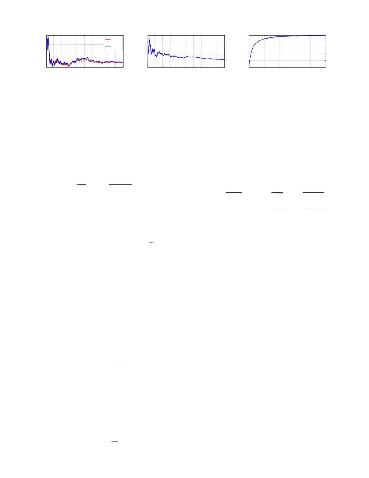
1 Nearly Consistent Finite P article Estimates in Streaming Importance Sampling Alec K oppel ∗ , Amrit Singh Bedi ∗ , Brian M. Sadler ∗ , and V ´ ıctor Elvira † Abstract —In Bayesian infer ence, we seek to compute inf or - mation about random variables such as moments or quantiles on the basis of av ailable data and prior information. When the distribution of random variables is intractable, Monte Carlo (MC) sampling is usually requir ed. Importance sampling is a standard MC tool that approximates this unavailable distrib ution with a set of weighted samples. This procedur e is asymptotically consistent as the number of MC samples (particles) go to infinity . Howev er , retaining infinitely many particles is intractable. Thus, we propose a way to only keep a finite representative subset of particles and their augmented importance weights that is nearly consistent . T o do so in an online manner , we (1) embed the posterior density estimate in a reproducing kernel Hilbert space (RKHS) through its kernel mean embedding; and (2) sequentially project this RKHS element onto a lower -dimensional subspace in RKHS using the maximum mean discrepancy , an integral probability metric. Theoretically , we establish that this scheme results in a bias determined by a compression parameter , which yields a tunable tradeoff between consistency and memory . In experiments, we observe the compr essed estimates achieve comparable performance to the dense ones with substantial reductions in repr esentational complexity . I . I N T R O D UC T I O N Bayesian inference is de v oted to estimating unkno wns by considering as them random variables and constructing a posterior distribution. This posterior distribution incorporates the information of a vailable observ ations (likelihood function) which is merged with prior kno wledge about the unknown (prior distrib ution) [3]. Its application is widespread, spanning statistics [4], signal processing [5], machine learning [6], genetics [7], communications [8], econometrics [9], robotics [10], among many other examples. Bayesian inference is only possible in a v ery small subset of problems (e.g., when the underlying model between observations and the hidden state is linear and corrupted by Gaussian noise [11]). In some cases, it is possible to linearize nonlinear models and still obtain closed-form (but approximate) solutions [12]. Beyond linear- ity , Bayesian inference may be tackled by Gaussian Processes when smoothness and unimodality are present [13]. Ho wev er , in most models of interest, closeed-form expressions are not av ailable, and the posterior distrib ution of the unknowns must be approximated. The standard approximation methodologies in Bayesian inference are either (a) Monte Carlo (MC) algorithms [14], A. K oppel and A.S. Bedi contributed equally to this work. A preliminary version of this work has appeared as [1], [2] with no proofs and a different (heuristic) projection rule for quantifying the difference between distrib utions. ∗ U.S. Army Research Laboratory , Adelphi, MD 20783, USA. E-mails: { alec.e.koppel.ci v , brian.m.sadler6.civ } @mail.mil, amrit0714@gmail.com † School of Mathematics, Univ ersity of Edinburgh, Peter Guthrie T ait Road, Edinbur gh, EH9 3FD United Kingdom: victor .elvira@ed.ac.uk which include Markov chain Monte Carlo (MCMC) methods [15], importance sampling (IS) [16], and particle filters (PFs) [17]; or (b) v ariational algorithms [18]. The later approach approximates the posterior by using an optimization algorithm to select within a parametrized family (e.g., by minimizing the KL div ergence). V ariational algorithms can optimize the parameters sequentially via the solution of a stochastic opti- mization problem [19]. In recent years, efforts to approximate the expectation by sampling hav e been in vestigated, e.g., see [20]. Unfortunately , unless the prior belongs to a simple exponential family , the parametric update is defined by a non- con ve x objectiv e, meaning that asymptotic unbiasedness is mostly beyond reach. Mixture models have been considered [21], but their con ver gence is challenging to characterize and the subject of recent work on resampling [22]. In contrast, MC is a general approach to Bayesian inference based upon sampling (i.e., the simulation of samples/particles), and is known to generate (weighted) samples that ev entually con ver ge to the true distribution/quantity of interest [23], [24]. Howe ver , the scalability of Monte Carlo methods is still an ongoing challenge from se v eral angles, in that to obtain consistency , the number of particles must go to infinity , and typically its scaling is exponential in the parameter dimension [25]. These scalability problems are the focus of this work, which we specifically study in the context of importance sampling (IS), a very relev ant family of MC methods. W e focus on IS, as compared with Marko v chain Monte Carlo (MCMC), due to advantages such as, e.g., no burn-in period, simple parallelization [26], built-in approximation of the nor- malizing constant that is useful in many practical problems (e.g., model selection), and the ability to incorporate adaptive mechanisms without compromising its conv ergence [27]. IS methods approximate expectations of arbitrary functions of the unknown parameter via weighted samples generated from one or sev eral proposal densities [28], [16]. Their con ver gence in terms of the integral approximation error , which vanishes as the number of samples increases, has been a topic of interest recently [28], [23], and various statistics to quantify their performance have been proposed [29]. Our goal is to alleviate the dependence of the conv ergence rate on the representational complexity of the posterior esti- mate. T o do so, we propose projecting the posterior density onto a finite statistically significant subset of particles after ev ery particle is generated. 1 Howe v er , doing so directly in a measure space is often intractable to ev aluate. By embedding 1 Doing so may be generalized to scenarios where projection can be performed after generating a fixed number T of particles, a form of mini- batching, b ut this is omitted for simplicity . 2 this density in a reproducing kernel Hilbert space (RKHS) via its kernel mean embedding [30], we may compute projections of distributions via parametric computations in volving the RKHS. More specifically , kernel mean embeddings extend the idea of feature mapping to spaces of probability distributions, which, under some re gularity conditions [30, Sec. 3.8], ad- mits a bijection between probability distributions and RKHS elements. Contributions. Based upon this insight, we propose a com- pression scheme that operates online within importance sam- pling, sequentially deciding which particles are statistically significant for the integral estimation. T o do so, we in vok e the idea of distribution embedding [30] and map our unnormalized distributional estimates to RKHS, in contrast to [31], [32]. W e show that the empirical kernel mean embedding estimates in RKHS are parameterized by the importance weights and particles. Then, we propose to sequentially project embed- ding estimates onto subspaces of the dictionary of particles, where the dictionary is greedily selected to ensure compressed estimates are close to the uncompressed one (according to some metric). This greedy selection is achiev ed with a custom variant of matching pursuit [33] based upon the Maximum Mean Discrepancy , which is an easily computable way to ev aluate an integral probability metric by virtue of the RKHS mean embedding. The underpinning of this idea is similar to gradient projections in optimization, which has been exploited recently to surmount memory challenges in kernel and Gaus- sian process regression [34], [35]. W e establish that the asymptotic bias of this method is a tunable constant depending on the compression parameter . These results yield an approach to importance reweighting that mitigates particle degeneracy , i.e., retaining a large number of particles with small weights [36], by directly compressing the embedding estimate of the posterior in the RKHS domain, rather than statistical tests that require sub-sampling in the distributional space [27], [37]. The compression is performed online , without waiting until the total number of samples N are av ailable, which is typically impractical. Experiments demonstrate that this approach yields an effecti ve tradeoff of consistency and memory , in contrast to the classical curse of dimensionality of MC methods. Additional Context. Dimensionality reduction of nonparamet- ric estimators been studied in disparate conte xts. A number of works fix the sparsity dimension and seek the best N - term approximation in terms of estimation error . When a likelihood model is av ailable, one terms the resulting active set a Bayesian cor esets [38]. Related approaches called “herding” assume a fixed number of particles and characterize the resulting error in a kernel-smoothed density approximation [39], [40], [41], [42]. In these works, little guidance is provided on how to determine the number of points to retain. In contrast, dynamic memory methods automatically tune the number of particles to ensure small model bias. For instance, in [43], a rule for retainment based on gradient pro- jection error (assuming the likelihood is av ailable) is proposed, similar to those arising in kernel regression [35]. Most similar to our work is the setting where a lik elihood/loss is unav ailable and one must resort to metrics on density estimates, i.e., sta- tistical tests, for whether new particles are significant. Specif- ically , in particle filters, multinomial resampling schemes can be used with Chi-squared tests to determine whether the cur- rent number of particles should increase/decrease [44], [45]. The performance of these approaches have only characterized when their b udget parameter goes to null or sparsity dimension goes to infinity . In contrast, in this w ork, we are especially focused on finite-sample analysis when budget parameters are left fixed, in order to elucidate the tradeoffs between memory and consistency , both in theory and practice. I I . E L E M E N T S O F I M P O RTA N C E S A M P L I N G In Bayesian inference [46][Ch. 7], we are interested in computing expectations I ( φ ) := E x [ φ ( x )   y 1: K ] = Z x ∈X φ ( x ) p ( x | y 1: K ) d x (1) on the basis of a set of av ailable observ ations y 1: K := { y 1: K } K k =1 , where φ : X → R is an arbitrary function, x is a random v ariable taking values in X ⊂ R p which is typically interpreted as a hidden parameter, and y is some observation process whose realizations y 1: K are assumed to be informati ve about parameter x . For e xample, φ ( x ) = x yields the computation of the posterior mean, and φ ( x ) = x p denotes the p -th moment. In particular , define the posterior density 2 p  x   y 1: K  = p  y 1: K   x  p ( x ) p ( y 1: K ) . (2) W e seek to infer the posterior (2) with K data points y 1: K av ailable at the outset. Even for this setting, estimating (2) has unbounded complexity [47], [48] when the form of the posterior is unknown. Thus, we prioritize efficient estimates of (2) from an online stream of samples from an importance density to be subsequently defined. Begin by defining posterior q ( x ) and un-normalized posterior e q ( x ) as q ( x ) = e q ( x ) / Z , e q ( x ):= e q ( x   y 1: K )= p  y 1: K   x  p ( x ) , (3) where e q ( x ) integrates to normalizing constant Z := p ( y 1: K ) 3 . In most applications, we only hav e access to a collection of observations y 1: K drawn from a static conditional density p ( y 1: K   x ) and a prior for p ( x ) . Therefore, the inte gral (1) cannot be ev aluated, and hence one must resort to numerical integration such as Monte Carlo methods. In Monte Carlo, we approximate (1) by sampling. Hypothetically , we could draw N samples x ( n ) ∼ q ( x ) and estimate the expectation in (1) by the sample average E q ( x ) [ φ ( x )] ≈ 1 N N X n =1 φ ( x ( n )) , (4) but typically it is difficult to obtain samples x ( n ) from posterior q ( x ) of the random variable. T o circumvent this 2 Throughout, densities are with respect to the Lebesgue measure on R p . 3 Note that q ( x ) and e q ( x ) depend on the data { y 1: K } k ≤ K , although we drop the dependence to ease notation. 3 issue, define the importance density π ( x ) 4 with the same (or larger) support as true density q ( x ) , and multiply and divide by π ( x ) inside the integral (1), yielding Z x ∈X φ ( x ) q ( x ) d x = Z x ∈X φ ( x ) q ( x ) π ( x ) π ( x ) d x , (5) where the ratio q ( x ) /π ( x ) is the Radon-Nikodym deriv ati ve, or unnormalized density , of the target q with respect to the proposal π . Then, rather than requiring samples from the true posterior , one may sample from the importance density x ( n ) ∼ π ( x ) , n = 1 , ..., N , and approximate (1) as I N ( φ ) := 1 N N X n =1 q ( x ( n )) π ( x ( n )) φ ( x ( n )) = 1 N Z N X n =1 g ( x ( n )) φ ( x ( n )) , (6) where g ( x ( n )) ≡ e q ( x ( n )) π ( x ( n )) , (7) are the importance weights. Note that (6) is unbiased, i.e., E π ( x ) [ I N ( φ )] = E q ( x ) [ φ ( x )] and consistent with N . Moreo ver , its variance depends on the importance density π ( x ) approx- imation of the posterior [16]. Example priors and measurement models include Gaussian, Student’ s t, and uniform. Which choice is appropriate depends on the context [46]. The normalizing constant Z can be also estimated with IS as ˆ Z := 1 N N X n =1 g ( x ( n )) . (8) Note that in Eq. (6), the unknown Z can be replaced by ˆ Z in 8. Then, the new estimator is giv en by I N ( φ ) := 1 N ˆ Z N X n =1 g ( x ( n )) φ ( x ( n )) (9) = 1 P N j =1 g ( x ( j )) N X n =1 g ( x ( n )) φ ( x ( n )) = N X n =1 w ( n ) φ ( x ( n )) , where the normalized w ( n ) weights are defined w ( n ) ≡ g ( x ( n )) P N u =1 g ( x ( u )) , (10) for all n . The whole IS procedure is summarized in Algorithm 1. The function I N ( φ ) is the normalized importance sampling (NIS) estimator . It is important to note that the estimator I N ( φ ) can be viewed as integrating a function φ with respect to density µ N defined as µ N ( x ) := N X n =1 w ( n ) δ x ( n ) , (11) 4 In general, the importance density could be defined over an y obser- vation process π ( x   { y k } ) , not necessarily associated with time indices k = 1 , . . . , K . W e define it this way for simplicity . Algorithm 1 IS: Importance Sampling with streaming samples Require: Observation model p ( y   x ) and prior p ( x ) or target density q ( x ) (if kno wn), importance density π ( x ) . Set of observations { y 1: K } K k =1 . for N = 0 , 1 , 2 , . . . do Simulate one sample from importance dist. x ( n ) ∼ π ( x ) Compute weight g ( x ( n )) [cf. (6)] Compute normalized weights w ( n ) by di viding by esti- mate for summand (8): w ( n ) = g ( x ( n )) P N u =1 g ( x ( u )) for all n. Estimate the expectation with the self-normalized IS as I N ( φ ) = N X n =1 w ( n ) φ ( x ( n )) The posterior density estimate is giv en by µ N = N X n =1 w ( n ) δ x ( n ) end for which is called the particle approximation of q . Here δ x ( n ) denotes the Dirac delta measure ev aluated at x ( n ) . This delta expansion is one reason importance sampling is also referred to as a histogram filter, as they quantify weighted counts of samples across the space. Subsequently , we leav e the argument (an ev ent, or measurable subset) of the delta δ x ( n ) as implicit. As stated in [28], [24], [23], for consistent estimates of (1), we require that N , the number of samples x ( n ) generated from the importance density , and hence the parameterization of the importance density , to go to infinity N → ∞ . There- fore, when we generate an infinite stream of particles, the parameterization of the importance density grows unbounded as it accumulates ev ery particle previously generated. W e are interested in allowing N , the number of particles, to become large (possibly infinite), while the importance density’ s com- plexity is moderate, thus overcoming an instance of the curse of dimensionality in Monte Carlo methods. In the next section, we propose a method to do so. I I I . C O M P R E S S I N G T H E I M P O RTA N CE D I S T R I B U T I O N In this section, we detail our proposed sequential compres- sion scheme for ov ercoming the curse of dimensionality in importance sampling. Ho wev er , to de velop such a compression scheme, we first re write importance sampling estimates in vector notation to illuminate the dependence on the number of past particles generated. Then, because directly defining projections over measure spaces is intractable, we incorporate a distributional approximation called a mean embedding [30], ov er which metrics can be easily e valuated. This permits us to develop our main projection operator . Begin by noting the curse of dimensionality in importance sampling can be succinctly encapsulated by rewriting the last step of Algorithm 1 in vector notation. Specifically , define g n ∈ R n , w n ∈ R n and X n = [ x (1); · · · x ( n )] ∈ R p × n . 4 Fig. 1: Approximating the distributions via kernel mean embedding. Then, after each new sample x ( n ) is generated from the importance distribution, we incorporate it into the empirical measure (11) through the parameter updates g n =[ g n − 1 ; g ( x ( n ))] , w n = z n g n , X n = [ X n − 1 ; x ( n )] , (12) where we define z n := 1 / ( 1 T n g n ) and 1 n is the all ones column vector with dimension n . The unnormalized posterior density estimate parameterized by g n and dictionary X n is giv en by ˜ µ n = n X u =1 g n ( u ) δ x ( u ) , (13) where we define g n ( u ) := g ( x ( u )) is the importance weight (6) and δ x ( u ) is the Dirac delta function, both ev aluated at sample x ( u ) . Denote as Ω X n the measure space “spanned” by Dirac measures centered at the samples stored in dictionary X n . More specifically , giv en measurable space (Ω , Σ , λ ) , where Ω is a set of outcomes, Σ is a σ -algebra whose elements are subsets, and λ : Σ → R denotes the Lebesgue measure, we define the restricted σ -algebra as Σ X n = { F ∩ { x ( u ) } u ≤ n : F ∈ Σ } . The measure space associated with Σ X n and the Lebesgue measure λ X n ov er this restricted σ -algebra we denote in shorthand as Ω X n (see [49] for more details). W e note that the unnormalized posterior density in (13) is a linear combination of (nonnegati ve) Dirac measures with mass g n ( u ) for each sample x ( u ) . The question is how to select a subset of columns of X n and modify the weights g n such that with an infinite stream of x ( n ) , we ensures the number of columns of X n is finite and the empirical integral estimate tends to its population counterpart, i.e., the integral estimation error becomes very small (or goes to zero) as n tends to infinity [50]. Henceforth, we refer to the number of columns in matrix X n which parameterizes (13) as the model order denoted by M n . A. K ernel Mean Embedding In this subsection, we introduce kernel mean embedding which maps the measure estimate in the measure space Ω X n to the corresponding reproducing kernel Hilbert space (RKHS) denoted by H X n as shown in Fig. 1. There is a kernel associated with with RKHS defined as κ : X × X → R and κ ( x , · ) ∈ H X n . In order to appropriately select a subset of X n which w ould define an approximator for ˜ µ n in (13), we emplo y the notion of kernel mean embedding [30] of Dirac measures, and then perform approximation in the corresponding RKHS H X n . Doing so is motiv ated by the fact that operations inv olv- ing distributions embedded in the RKHS may be ev aluated in closed form, whereas in general measure spaces it is often intractable. The explicit value of the map for ˜ µ n to RKHS is giv en by β n = n X u =1 g n ( u ) κ ( x ( u ) , · ) , (14) and β n ∈ H X n . W e remark here that the associated kernel κ with RKHS is assumed to be a characteristic kernel which ensure that the mapping ˜ µ n → β n is injectiv e [51, Def. 3.2]. A characteristic kernel is imperative to make sure that k β P − β Q k H = 0 if and only if P = Q for measures P and Q , i.e., that it satisfies the identity of indiscernibles. This makes sure that there is no information loss by introducing the mapping via kernel mean embedding. For practical purpose, we are interested in obtaining the value of the underlying posterior density associated with the mean embedding, which necessitates a way to inv ert the embedding. Doing so is achiev able by computing the distributional pre-image [52], which for a given β n ∈ H X n is given by g ? := argmin g ∈ R n    β n − n X u =1 g ( u ) κ ( x ( u ) , · )    2 H , (15) where P n u =1 g ( u ) κ ( x ( u ) , · ) is the kernel mean embedding for the Dirac measure P n u =1 g ( u ) δ d x ( u ) and g = g ? is obtained as the solution of (15). Therefore, for a giv en β n ∈ H X n , we could reco ver the corresponding distrib ution in the measure space Ω X n by solving (15). Note that (15) exhibits a closed form solution with g ? = g n , as the distributional measures hav e a Dirac measure structure. This motiv ates us to perform the compression in the RKHS H X n parameterized by X n . Specifically , giv en past particles collected in a dictionary X n , we seek to select the subset of columns of X n to formulate its compressed variant D n . W e propose to project the kernel mean embedding β n onto subspaces H D n = span { κ ( d u , · ) } M n u =1 that consist only of functions that can be represented using dictionary D n = [ d 1 , . . . , d M n ] ∈ R p × M n . More precisely , H D n is defined as a subspace in the RKHS H X n that can be expressed as a linear combination of kernel ev aluations at points { d u } M n u =1 . W e enforce efficienc y by selecting dictionaries D n such that M n  n . The ev entual goal is to achieve a finite memory M n = O (1) as n → ∞ or M n n → 0 as n → ∞ , while ensuring the underlying integral estimate has minimal bias, i.e., that we can obtain nearly consistent finite particle estimates. B. Gr eedy Subspace Pr ojections Next, we de velop a way to only retain statistically sig- nificant particles by appealing to ideas from subspace based projections [53], inspired by [35], [34]. T o do so, we begin by rewriting the evolution of the mean embedding in (14) as β n = β n − 1 + g n ( n ) κ ( x ( n ) , · ) . (16) W e note that the update in (16) can be written as β n = argmin f ∈H X n k f −  β n − 1 + g n ( n ) κ ( x ( n ) , · )  k 2 H , (17) 5 Algorithm 2 Compressed Kernelized IS (CKIS) Require: Unnormalized tar get distribution e q ( x ) , importance distribution π ( x ) . for n = 0 , 1 , 2 , . . . , N do Simulate one sample from importance dist. x ( n ) ∼ π ( x ) Compute the importance weight g ( x ( n )) ≡ ˜ q ( x ( n )) π ( x ( n )) Normalize weights w ( n ) by estimate for summand (8): w ( j ) := w ( j ) z n , j = 1 , ..., n. , z n = n X u =1 w ( u ) Update the mean embedding via last sample & weight [cf. (16)] ˜ β n = β n − 1 + g n ( n ) κ ( x ( n ) , · ) . Append dictionary ˜ D n = [ D n − 1 ; x ( n )] and importance weights ˜ g n = [ g n − 1 ; g ( x ( n ))] Compress the mean embedding as (cf. Algorithm 3) ( β n , D n , g n ) = MMD-OMP ( ˜ β n , ˜ D n , ˜ g n ,  n ) Evaluate the pre-image to calculate ˆ µ n using (15) Estimate the expectation as ˆ I n = P | D n | u =1 w ( u ) φ ( x ( u )) end for where the equality employs the fact that β n can be represented using only the elements in H X n = span { κ ( x ( u ) , · ) } u ≤ n . Observe that (17) defines a projection of the update  β ˜ µ n − 1 + g n ( n ) κ ( x ( n ) , · )  onto the subspace defined by H X n , which we propose to replace at each iteration by a projection onto a subspace defined by dictionary D n , which is extracted from the particles observed thus far . The process by which we select D n will be discussed next. T o be precise, we replace the update (17) in which the number of particles grows at each step by the subspace projection onto H D n as β n = argmin f ∈H D n k f −  β ˜ µ n − 1 + g n ( n ) κ ( x ( n ) , · )  k 2 H := P H D n [ β n − 1 + g n ( n ) κ ( x ( n ) , · )] . (18) Let us define ˜ β n := β n − 1 + g n ( n ) κ ( x ( n ) , · ) , which means that β n = P H D n [ ˜ β n ] . Let us denote the corresponding dictionary update as ˜ g n =[ g n − 1 ; g ( x ( n ))] , ˜ D n = [ D n − 1 ; x ( n )] w n = z n g n , (19) where D n − 1 has M n − 1 number of elements and ˜ D n has ˜ M n = M n − 1 + 1 . Using the expression for mean embedding in (14), we may write the projection in (18) as follo ws g n := argmin g ∈ R M n    M n X s =1 g ( s ) κ ( d s , · ) − ˜ M n X u =1 ˜ g n ( u ) κ ( ˜ d u , · )    2 H (20) = argmin g ∈ R M n  g T K D n , D n g − 2 g T K D n , ˜ D n ˜ g n + ˜ g n K ˜ D n , ˜ D n ˜ g n  , where we expand the square and define the kernel cov ariance matrix K D n , ˜ D n whose ( s, u ) th entry is given by κ ( d s , ˜ d u ) . The other matrices K ˜ D n , ˜ D n and K D n , D n are similarly de- fined. The problem in (20) may be solved explicitly by Algorithm 3 MMD based Orthogonal Matching Pursuit (MMD-OMP) Require: kernel mean embedding ˜ β n defined by dict. ˜ D n ∈ R p × ˜ M n , coeffs. ˜ g ∈ R ˜ M n , approx. budget  n > 0 initialize β = ˜ β n , dictionary D = ˜ D n with indices I , model order M = ˜ M n , coeffs. g = ˜ g n . while candidate dictionary is non-empty I 6 = ∅ do for j = 1 , . . . , M do Find minimal approx. error with dictionary element d j remov ed γ j = MMD h ˜ β n , X k ∈I \{ j } g ( k ) κ ( d k , · ) i . end for Find dictionary index minimizing approximation error: j ? = arg min j ∈I γ j if minimal approx. error exceeds threshold γ j ? >  n stop else Prune dictionary D ← D I \{ j ? } , remov e the columns associated with index j ? Revise set I ← I \ { j ? } and model order M ← M − 1 . Update weights g defined by current dictionary D g = argmin w ∈ R M   ˜ β n − M X u =1 w ( u ) κ ( d u , · )   H end end while Assign g n = g and Ev aluate the projected kernel mean embedding as β n = P M u =1 g n ( u ) κ ( d u , · ) retur n β n , D n , g n of complexity M ≤ ˜ M s.t. MMD [ ˜ β n , β n ] ≤  n computing gradients and solving for g n to obtain g n = K − 1 D n , D n K D n ˜ D n ˜ g n . (21) Then, the projected estimate of the mean embedding ˜ β n is giv en by β n = P H D n [ ˜ β n ] = M n X s =1 g n ( s ) κ ( d s , · ) , (22) where g n is obtained as a solution to (21). Now , for a gi ven dictionary D n , we know how to obtain the projected version of the mean embedding for each n . Next, we discuss the procedure to obtain D n at each n . C. Dictionary Update The selection procedure for the dictionary D n is based upon greedy sparse approximation, a topic studied in compressi ve sensing [54]. The function ˜ β n := β n − 1 + g n ( n ) κ ( x ( n ) , · ) is parameterized by dictionary ˜ D n , whose model order is ˜ M n = M n − 1 + 1 . W e form D n by selecting a subset of M n columns from ˜ D n that are best for approximating the kernel mean embedding ˜ β n in terms of maximum mean discrepancy (MMD). As previously noted, numerous approaches are pos- sible for sparse representation. W e make use of destructi ve 6 orthogonal matching pursuit (OMP) [55] with allowed error tolerance  n to find a dictionary matrix D n based on the one that includes the latest sample point ˜ D n . W ith this choice, we can tune the stopping criterion to guarantee the per-step estimates of mean embedding are close to each other . W e name the compression procedure MMD-OMP and it is summarized in Algorithm 3. From the procedure in Algorithm 3, note that the projection operation in (18) is performed in a manner that ensures that MMD [ ˜ β n , β n ] ≤  n for all n , and we recall that β n is the compressed version of ˜ β n . I V . B A L A N C I NG C O N S I S T E N C Y A N D M E M O RY In this section, we characterize the conv ergence behavior of our posterior compression scheme. Specifically , we establish conditions under which the asymptotic bias is proportional to the kernel bandwidth and the compression parameter using posterior distrib utions giv en by Algorithm 2. T o frame the discussion, we note that the NIS estimator (9) I N ( φ ) , whose particle complexity goes to infinity , is asymptotically consis- tent [56][Ch. 9, Theorem 9.2], and that the empirical posterior µ N ( · ) contracts to its population analogue at a O (1 / N ) rate where N is the number of particles. T o establish consistency , we first detail the technical conditions required. A. Assumptions and T echnical Conditions Assumption 1 Recall the definition of the tar get distrib ution q fr om Sec. II (following (2) ). Denote the inte gral of test function φ : X → R as q ( φ ) . (i) Assume that φ is absolutely integr able, i.e., q ( | φ | ) < ∞ , and has absolute value at most unit | φ | ≤ 1 . (ii) The test function has absolutely continuous second derivative, and R x ∈X φ 00 ( x ) d x < ∞ . Assumption 2 The kernel function associated with RKHS is such that R x ∈X κ x ( n ) ( x ) = 1 , R x ∈X x κ x ( n ) ( x ) = 0 , and σ 2 κ = R x ∈X x 2 κ x ( n ) ( x ) > 0 . Assumption 3 Let I N ( φ ) and ˆ I N ( φ ) be the inte gral estima- tors for test function φ associated with the uncompr essed and compr essed posterior densities. W e define the appr oximation err or for φ / ∈ F wher e F := { f ∈ H | k f k H ≤ 1 } , as I ( φ, f ) = sup | φ |≤ 1  E [ ˆ I N ( φ ) − I N ( φ )]  − sup f ∈F  E [ ˆ I N ( f ) − I N ( f )]  , (23) W e assume that I ( φ, f ) ≤ G , where G is a finite constant. Assumption 1(i) is a textbook condition in the analysis of Monte Carlo methods, and appears in [56]. Assumptions 1(ii) and 2 are required conditions for establishing consistency of kernel density estimates and are standard – see [57][Theorem 6.28]. W e begin by noting that under Assumption 1, we hav e classical statistical consistency of importance sampling as the number of particles becomes large as stated in Lemma 2 in Appendix A. This result enables characterizing the bias of Algorithm 2, given next in Lemma 1. Assumption 3 is non- standard and we use it to bound the error due to continuity conditions imposed by operating in the RKHS. W e note that if φ ∈ F which is the case for most practical applications, then G = 0 . Lemma 1 Define the second moment of the true unnormalized density ρ as in Lemma 2. Then, under Assumptions 1-3, the estimator of Alg. 2 satisfies   sup | φ |≤ 1  E [ ˆ I N ( φ ) − I ( φ )]    ≤ N X n =1  n + 24 N ρ + G. (24) wher e  n is the compression budget for each n . Proof : Inspired by [23], begin by denoting ˆ I N ( φ ) as the integral estimate giv en by Algorithm 2. Consider the bias of the integral estimate ˆ I N ( φ ) − I ( φ ) , and add and subtract I N ( φ ) , the uncompressed normalized importance estimator that is the result of Algorithm 1, to obtain ˆ I N ( φ ) − I ( φ ) = ˆ I N ( φ ) − I N ( φ ) + I N ( φ ) − I ( φ ) . (25) T ake the expectation on both sides with respect to the popu- lation posterior (2) to obtain E [ ˆ I N ( φ ) − I ( φ )] = E [ ˆ I N ( φ ) − I N ( φ )] + E [ I N ( φ ) − I ( φ )] . (26) Let’ s compute the sup of both sides of (26) over range | φ | ≤ 1 and use the fact that a sup of a sum is upper-bounded by the sum of individual terms: sup | φ |≤ 1  E [ ˆ I N ( φ ) − I ( φ )]  ≤ sup | φ |≤ 1  E [ ˆ I N ( φ ) − I N ( φ )]  + sup | φ |≤ 1 ([ E [ I N ( φ ) − I ( φ )]) . (27) Now add and subtract the supremum ov er the space F := { f ∈ H | k f k H ≤ 1 } to the first term on the right hand side of (27) to write sup | φ |≤ 1  E [ ˆ I N ( φ ) − I ( φ )]  (28) ≤ sup f ∈F  E [ ˆ I N ( f ) − I N ( f )]  + sup | φ |≤ 1 ([ E [ I N ( φ ) − I ( φ )]) + sup | φ |≤ 1  E [ ˆ I N ( φ ) − I N ( φ )]  − sup f ∈F  E [ ˆ I N ( f ) − I N ( f )]  | {z } I ( φ,f ) ≤ G Observe that the last line on the right-hand side of the pre- ceding expression defines the integral function approximation error I ( φ, f ) defined in (23), which is upper-bounded by constant G (Assumption 3). Now , compute the absolute value of both sides of (28), and to the second term on the first line, pull the absolute value inside the supremum. Doing so allows us to apply (49) (Lemma 2) to the second term on the first line, the result of which is:   sup | φ |≤ 1  E [ ˆ I N ( φ ) − I ( φ )]    ≤ sup f ∈F  E [ ˆ I N ( f ) − I N ( f )]  + 24 N ρ + G, (29) where G is defined in Assumption 3 and note that G = 0 if φ ∈ H . It remains to address the first term on the right 7 hand side of (29), which noticeably defines an instance of an integral probability metric (IPM) [Muller 1997], i.e., sup f ∈F  E [ ˆ I N ( f ) − I N ( f )]  = sup f ∈F  Z f ( x ) d ˆ µ N − Z f ( x ) d ˜ µ N  , (30) where ˆ µ N is the pre-image unnormalized density estimate obtained by solving (15). The IPM in (30) is exactly equal to Maximum Mean Discrepancy (MMD)[58] for test functions in the RKHS f ∈ H . This observation allows us to write sup f ∈F  E [ ˆ I N ( f ) − I N ( f )]  = k β N − γ N k H . (31) where γ N is the kernel mean embedding corresponding to the uncompressed measure estimate ˜ µ N . Next, consider the term k β N − γ N k H and add and subtract the per step uncompressed estimate ˜ β N [cf. (19)] to obtain k β N − γ N k H = k ( β N − ˜ β N ) + ( ˜ β N − γ N ) k H ≤k β N − ˜ β N k H + k ˜ β N − γ ν N k H ≤  N + k ˜ β N − γ N k H , (32) where the last inequality holds from the fact that k β N − ˜ β N k H ≤  N (cf. Algorithm 3). Now we substitute the values of ˜ β N and γ N using the update in (16), and we get k β N − γ N k H ≤  N + k β N − 1 − γ N − 1 k H . (33) Using the above recursion, we easily obtain k β N − γ N k H ≤ N X n =1  n . (34) Hence, using the upper bound of (34) in (31), and then substituting the result into (29) yields   sup | φ |≤ 1  E [ ˆ I N ( φ ) − I ( φ )]    ≤ N X n =1  n + 24 N ρ + G. (35) as stated in Lemma 1.  W ith this technical lemma in place, we are ready to state the main result of this paper . Theorem 1 Define ρ = π ( g 2 ) q ( g 2 ) as the variance of the unnor- malized importance density with r espect to importance weights g as in Lemma 2. Then under Assumptions 1-3, we have the following approximate consistency r esults: (i) for diminishing compression budget  n = α n with α ∈ (0 , 1) , the estimator of Alg. 2 satisfies   sup | φ |≤ 1  E [ ˆ I N ( φ ) − I ( φ )]    ≤ α 1 − α + O  1 N  + G. (36) T o obtain a δ accurate inte gral estimate, we need at least N ≥ O  1 δ  particles and compr ession attenuation rate sufficiently lar ge such that 0 < α ≤ 1 / (1 + (2 /δ )) . (ii) for constant compr ession budget  n =  > 0 and memory M := O  1  1 / (2 p )    sup | φ |≤ 1  E [ ˆ I N ( φ ) − I ( φ )]    ≤ O  N M 1 / 2 p + 1 N  (37) and O  1 δ  ≤ N ≤ O  δ M 1 / (2 p )  , (38) which implies that M ≥ O  1 δ 4 p  . Proof : Consider the statement of Lemma 24 and to proceed next, we characterize the beha vior of the term P N n =1  n since it ev entually determines the final bias in the integral estimation. Theorem 1(i) : Diminishing compression budget: Let us con- sider  n = ( α ) n with α = (0 , 1) , which implies that N X n =1  n = α (1 − α N ) 1 − α ≤ α 1 − α . (39) Substituting (39) into the right hand side of (35), we get   sup | φ |≤ 1  E [ ˆ I N ( φ ) − I ( φ )]    ≤ α 1 − α + 24 N ρ. (40) T o obtain a δ accurate integral estimate, we need N ≥ 48 ρ δ and 0 < α ≤ 1 / (1 + (2 /δ )) . Theorem 1(ii) : Constant compression budget: Let us consider  n =  , which implies that N X n =1  n = N . (41) Using (41) in (35), we can write   sup | φ |≤ 1  E [ ˆ I N ( φ ) − I ( φ )]    ≤ N  + 24 N ρ. (42) For a constant compression budget  , from Theorem 2, we hav e M ∞ ≤ O  1  2 p  := M . (43) If we are giv en a maximum memory requirement M , then we can choose  as  = G M 1 / (2 p ) , (44) where G is a bound on the unnomalized weight g ( x ( u )) ≤ G for all u . Using this lower bound value of  in (42), we get   sup | φ |≤ 1  E [ ˆ I N ( φ ) − I ( φ )]    ≤ N G M 1 / 2 p + 24 N ρ. (45) 0 2 4 6 8 10 x 0 0.05 0.1 p ( x ) Fig. 2: Particle histogram for direct sampling experiment. 8 100 200 300 400 500 600 700 800 900 1000 Iteration, n 0.5 0.51 0.52 0.53 ˆ I n IS CKIS (a) Integral estimate. 100 200 300 400 500 600 700 800 900 1000 Iteration, n 0 0.002 0.004 0.006 0.008 0.01 Approx. error (b) Integral Error between Algs. 1 - 2. 0 200 400 600 800 1000 Iteration, n 0 10 20 30 40 M n (c) Model Order . Fig. 3: Simulation results for Alg. 2 run with Gaussian kernel ( h = 0 . 01 ) and compression budget  = 3 . 5 for the problem (48). The memory- reduction scheme nearly preserves statistical consistency , while yielding reasonable complexity , whereas Alg. 1 attains exact consistency as its memory grows unbounded with index n . All the plots are averaged over 10 iterations. Note that the first term in the abov e expression increases with N and the second term decreases with N , hence we obtain a tradeof f between memory and accuracy for the importance sampling based estimator . For a given memory M (number of elements we could store in the dictionary) and the required accuracy δ , we obtain the following bound on the number of iterations N 48 ρ δ ≤ N ≤ δ M 1 / (2 p ) 2 G , (46) which implies that for increased accuracy we need to run for more iterations but need more memory , and vice versa.  Theorem 1 establishes that the compressed kernelized im- portance sampling scheme proposed in Section III is nearly asymptotically consistent. Note that the right hand side in (36) consists of three terms depending upon α , 1 N , and G . If we ignore G , which actually depends upon the approximation associated with function φ ( · ) , the other two terms can be made arbitrarily small by making α close to zero and a very high N . Hence, the integral estimation can be made arbitrarily close to exact integral. Ho wev er , when these parameters are fix ed positiv e constants, they provide a tunable tradeoff between bias and memory . That is, when the compression budget is a positiv e constant, then the memory of the posterior distribution representation is finite, as we formalize next. Theorem 2 Under Assumptions 1-2 (in Section IV -A), for compact featur e space X and bounded importance weights g ( x ( n ) ) , the model order M n for Algorithm 2, for all n is bounded by 1 ≤ M n ≤ O  1  2 p  . (47) Theorem 2 (proof in Appendix B) contrasts with the classical bottleneck in the number of particles required to represent an arbitrary posterior , which grows unbounded [23]. While this is a pessimistic estimate, experimentally we observe orders of magnitude reduction in complexity compared to exact importance sampling, which is the focus of the subsequent section. Observ e, ho wev er , that this memory-reduction does not come for free, as once the compression b udget is fixed, the memory is fixed by the ratio 1  2 p that e ventually results in a lower bound on the accuracy of the integral estimate. V . E X P E R I M E N T S A. Dir ect Importance Sampling In this section, we conduct a simple numerical experiment to demonstrate the efficac y of the proposed algorithm in terms of balancing model parsimony and statistical consistency . W e consider the problem of estimating the expected value of function φ ( x ) with the target q ( x ) and the proposal π ( x ) giv en by φ ( x ) = 2 sin  π (1 . 5 x )  , q ( x ) = 1 √ 2 π exp  − ( x − 1) 2 2  , π ( x ) = 1 √ 4 π exp  − ( x − 1) 2 4  , (48) to demonstrate that generic Monte Carlo inte gration allo ws one to track generic quantities of random variables that are dif ficult to compute under more typical probabilistic hypotheses. For (48), since q ( x ) is known, this is referred to as “direct impor- tance sampling”. W e run Algorithm 1, i.e., classic importance sampling, and Algorithm 2 for the aforementioned problem. For Algorithm 2, we select compression budget  = 3 , and used a Gaussian kernel with bandwidth h = 0 . 01 . W e track the normalized integral estimate (9), absolute integral approx- imation error , and the number of particles that parameterize the empirical measure (model order). W e first represent the histogram of the particles generated in Fig. 2. In Fig. 3a, we plot the un-normalized integral approximation error for Algorithms 1 - 2, which are close, and the magnitude of the dif ference depends on the choice of compression budget. V ery little error is incurred by kernel mean embedding and memory-reduction. The magnitude of the error relative to the number of particles generated is displayed in Fig. 3b: observe that the error settles on the order of 10 − 3 . In Fig. 3c, we display the number of particles retained by Algorithm 2, which stabilizes to around 56 , whereas the complexity of the empirical measure giv en by Algorithm 1 grows linearly with sample index n , which noticeably grows unbounded . B. Indir ect Importance Sampling As discussed in Sec. II, in practice we do not kno w the tar get distribution q ( x ) and hence we use Bayes rule as described in (7) to calculate q ( x ( n ) ) at each instant t . W e consider the observation model y t = b + sin (2 π x ) + η t where η t ∼ N (0 , σ 2 ) . From the equality in (7), we need the likelihood 9 0 500 1000 1500 Iteration, n -0.2 0 0.2 ˆ I n IS CKIS (a) Integral estimate. 0 500 1000 1500 Iteration, n 0 0.05 0.1 0.15 0.2 Approx. error (b) Integral Error between Algs. 1 - 2. 0 500 1000 1500 Iteration, n 0 10 20 30 40 M n (c) Model Order . Fig. 4: Simulation results for Alg. 2 with indirect IS, run with Gaussian kernel ( h = 0 . 012 ) and compression budget  = 10 − 3 for the problem (48). The memory-reduction scheme nearly preserves statistical consistency , while yielding reasonable complexity , whereas Alg. 1 attains exact consistency as its memory grows unbounded with index n . All the plots are averaged over 10 iterations. and a prior distribution to calculate q ( x ( n ) ) using Bayes Rule [cf. (2)]. Here we fix the likelihood (measurement model) and prior as P  { y k } k ≤ K   x ( n )  = 1 (2 π σ 2 1 ) K/ 2 exp  − k y − x ( n ) k 2 2 σ 2 1  , P  x ( n )  = 1 (2 π σ 2 2 ) exp  − ( x ( n ) ) 2 2 σ 2 2  . W e set K = 10 , b = 5 , σ = 0 . 1 , σ 1 = 0 . 4 , σ 2 = 1 . 6 , and compression budget  = 10 − 3 . A uniform distribution U [3 , 7] is used as the importance distribution. The results are reported in Fig. 4. W e observe a comparable tradeoff to that which may be gleaned from Section V: in particular, we are able to obtain complexity reduction by orders of magnitude with extremely little integral estimation error . This suggests the empirical validity of our compression-rule based on un-normalized importance weights operating in tandem with kernel smoothing. C. Sour ce Localization In this section we present a sensor network localization experiment based on range measurements.The results illustrate the ability to succinctly represent the unknown distribution of the source signal location, yielding a model that is both parsimonious and nearly consistent. Consider the problem of localizing a static target in two-dimensional space R 2 with range measurements from the source collected in a wireless sensor network (WSN). Since the observation model is non- linear , the posterior distribution of the location of the target is intractable, and hence finding the least-squares estimator is not enough. This problem is well-studied in signal processing [59] and robotics [60]. Let x = [ x, y ] T denote the random unknown tar get location. W e assume six sensors with locations { h i } 6 i =1 at locations [1 , − 8] T , [8 , 10] T , [ − 15 , − 17] T , [ − 8 , 1] T , [10 , 0] T , and [0 , 10] T , respecti vely . The true location of the target is at [3 . 5 , 3 . 5] T . The measurement at each sensor i is related to the true target location x via the following nonlinear function of range y i,j = − 20 log( k x − h i k ) + η i for i = 1 to 6 and j = 1 to N , where N i is the number of measurements collected by sensor i . Here, η i ∼ N (0 , 1) models the range estimation error . For the experiment, we consider a Gaussian prior on the target location x with mean [3 . 5 , 3 . 5] T and identity covariance matrix. W e use the actual target location as the mean for the Gaussian prior because we are interested in demonstrating that the proposed technique successfully balances particle growth and model bias. In practice, for a general possibly misspecified prior , we can appeal to advanced adaptiv e algorithms – for example see [37], [27]. Fig. 5 shows the performance of the proposed algorithm compared against classical (uncompressed) normalized impor- tance sampling. Fig. 5a shows that the final estimated value of the target location for compressed and uncompressed versions of the algorithms are close. W e plot the squared error in Fig. 5b and both algorithms conv erge with close limiting estimates. Further , in Fig. 5c we observe that the model order for the compressed distrib ution settles to 21 , whereas the classical algorithm requires its number of particles in its importance distribution to gro w unbounded. The memory-reduction comes at the cost of very little estimation error (Fig. 5a). V I . C O N C L U S I O N S W e focused on Bayesian inference where one streams simulated Monte Carlo samples to approximate an unknown posterior via importance sampling. Doing so may consistently approximate any function of the posterior at the cost of infinite memory . Thus, we proposed Algorithm 2 (CKIS) to approximate the posterior by a kernel density estimate (KDE) projected onto a nearby lo wer -dimensional subspace, which allows online compression as particles arriv e in perpetuity . W e established that the bias of CKIS depends on kernel band- width and compression b udget, providing a tradeoff between statistical accuracy and memory . Experiments demonstrated that we attain memory-reduction by orders of magnitude with very little estimation error . This motiv ates future application to memory-ef ficient versions of Monte Carlo approaches to nonlinear signal processing problems such as localization, which has been eschewed due to its computational burden. A P P E N D I X A P RO O F O F C O N S I S T E N C Y O F I M P O RTA N C E S A M P L I N G Here we state a result on the sample complexity and asymptotic consistency of IS estimators in terms of inte gral error . W e increase the granularity of the proof found in the literature so that the modifications required for our results on compressed IS estimates are laid bare. Lemma 2 [23][Theorem 2.1] Suppose π , the pr oposal distri- bution is absolutely continuous w .r .t. q , the population poste- rior , and both ar e defined over X . Then define their Radon- Nikodyn derivative: dq dπ ( x ) := g ( x ) R X g ( x ) π ( d x ) , ρ := π ( g 2 ) q ( g 2 ) wher e g is the unnormalized density of q with respect to π . Mor eover , ρ is its second moment (“variance” of unnormalized density). Under Assumption 1(i), Alg. 1 contracts to the true posterior as sup | φ |≤ 1 | E [ I N ( φ ) − I ( φ )] | ≤ 12 N ρ, E  ( I N ( φ ) − I ( φ )) 2  ≤ 4 N ρ , (49) 10 2.5 3 3.5 4 4.5 2.5 3 3.5 4 4.5 -900 -850 -800 -750 Compressed Uncompressed Target (a) Location estimate. 20 40 60 80 100 Iterations, t 0 0.05 0.1 0.15 0.2 Squared error Uncompressed Compressed (b) Squared error estimate. 0 20 40 60 80 100 Iterations, t 0 50 100 Model Order Uncompressed Compressed (c) Model Order . Fig. 5: Simulation results for Alg. 2 run with Gaussian kernel ( h = 0 . 0001 ) and compression budget  = 0 . 002 . Observe that the memory- reduction scheme (compressed) nearly preserves statistical consistency , while yielding a finite constant limiting model complexity , whereas the original uncompressed version (uncompressed) attains exact consistency but its memory grows linearly with particle index t . and hence approac hes exact consistency as N → ∞ . Proof : This is a more detailed proof than giv en in [23][Theorem 2.1] dev elop for greater completeness and co- herence. Let us denote the empirical random measure by π N as π N := 1 N N P n =1 δ x ( n ) , and x ( n ) ∼ π , where π N is the occupancy measure, which when weighted, yields the importance sampling empirical measure (11). Note that the integral approximation at N is denoted by I N ( φ ) . W ith the abov e notation is hand, it holds that π N ( g ) = Z 1 N N X n =1 g ( x ) δ x ( n ) ( x ) dx = 1 N N X n =1 g ( x ( n )) , (50) and similarly π N ( φg ) = Z 1 N N X n =1 δ x ( n ) ( x ) φ ( x ) g ( x ) dx = 1 N N X n =1 φ ( x ( n )) g ( x ( n )) . (51) From the above equalities, we can write the estimator bias as I N ( φ ) − I ( φ ) = π N ( φg ) π N ( g ) − I ( φ ) (52) = π N ( φg ) π N ( g ) −  I ( φ ) π N ( g ) π N ( g )  (53) = 1 π N ( g )  π N ( φg ) − I ( φ ) π N ( g )  (54) = 1 π N ( g ) π N (( φ − I ( φ )) g ) . (55) Let us define ¯ φ := φ − I ( φ ) and note that π ( ¯ φg ) = 0 . (56) Rewriting the bias, we get I N ( φ ) − I ( φ ) = 1 π N ( g ) π N  ¯ φg  = 1 π N ( g )  π N  ¯ φg  − π  ¯ φg  , (57) where the second equality holds from (56). The first term in the bracket is an unbiased estimator for the second one, so that E  π N  ¯ φg  − π  ¯ φg  = 0 . (58) T aking the expectation on both sides of (57), we get E [ I N ( φ ) − I ( φ )] = E  1 π N ( g )  π N  ¯ φg  − π  ¯ φg   . (59) Since it equals zero, we can add the expression in (58) to the right hand side of (59) to obtain E [ I N ( φ ) − I ( φ )] = E  1 π N ( g )  π N  ¯ φg  − π  ¯ φg   + E  π N  ¯ φg  − π  ¯ φg  (60) = E  1 π N ( g )  π N  ¯ φg  − π  ¯ φg   + E  1 π ( g )  π N  ¯ φg  − π  ¯ φg   . (61) T aking the expectation operator outside, we get E [ I N ( φ ) − I ( φ )] = E   1 π N ( g ) − 1 π ( g )   π N  ¯ φg  − π  ¯ φg   = E  1 π N ( g ) π ( g )  π ( g ) − π N ( g )   π N  ¯ φg  − π  ¯ φg   . (62) Next, we split the set of integration to A = { 2 π N M C ( g ) > π ( g ) } and its compliment using the property E [ f ( X )] = E [ f ( X )1 A ( X )] + E [ f ( X )1 A c ( X )] , where 1 A the indicator function of the set A selecting A = { 2 π N M C ( g ) > π ( g ) } , which takes v alue 1 if x ∈ A and 0 if x / ∈ A . W e get | E [ I N ( φ ) − I ( φ )] | ≤ | E [ I N ( φ ) − I ( φ )] 1 { 2 π N ( g ) >π ( g ) } | + | E [ I N ( φ ) − I ( φ )] 1 { 2 π N ( g ) ≤ π ( g ) } | . (63) Consider the second term of (63), and use the fact that | φ | ≤ 1 , and so | µ N ( φ ) | , | I ( φ ) | ≤ 1 since they are mean v alues w .r .t. probability measures µ N , q respectiv ely . Then we use E [1 A ] = P ( A ) and obtain | E [ I N ( φ ) − I ( φ )] | ≤| E [ I N ( φ ) − I ( φ )] 1 { 2 π N ( g ) >π ( g ) } | + 2 P  2 π N ( g ) ≤ π ( g )  . (64) The constant 2 comes from the fact that | I N ( φ ) − I ( φ ) | ≤ | I N ( φ ) | + | I ( φ ) | ≤ 2 . For the first term on the right hand side of (64), from the set condition (, it holds that 1 π N M C ( g ) π ( g ) < 2 π 2 ( g ) , (65) 11 which implies that | E [ I N ( φ ) − I ( φ )] | ≤ 2 π ( g ) 2 E  | π ( g ) − π N ( g ) || π N ( ¯ φg ) − π  ¯ φg  |  + 2 P  2 π N ( g ) ≤ π ( g )  . (66) Finally , to upper bound the first term on the right hand side of (66), we first bound the expectation using Cauchy-Schwartz E [ | π ( g ) − π N ( g ) || π N ( ¯ φg ) − π ( ¯ φg ) | ] ≤ E [( π ( g ) − π N ( g )) 2 ] 1 2 E [( π N ( ¯ φg ) − π ( g )) 2 ] 1 2 (67) The first expectation on the right hand side of (67) is bounded as follows: by definition of π N we have for x n ∼ π independent that E [( π ( g ) − π N ( g )) 2 ] = E [( π ( g ) − 1 N N X n =1 g ( x ( n )) 2 )] = 1 N 2 E [( N X n =1 g ( x ( n )) − N π ( g )) 2 ] , (68) which since E [ g ( x ( n ))] = π ( g ) and by independence of the x ( n ) is equal to = 1 N 2 V ar ( N X n =1 g ( x ( n ))) = 1 N 2 N X n =1 V ar ( g ( x ( n ))) , and since x ( n ) is identically distrib uted, x ( n ) ∼ π , this is equal to N N 2 V ar u ∼ π ( g ) = 1 N ( π ( g 2 ) − π ( g ) 2 ) ≤ 1 N π ( g 2 ) . The second expectation on the right hand side of (67) is bounded in a similar way along with the fact that | φ | ≤ 1 so that | ¯ φ | ≤ 2 . Then we utilize these upper bounds on the right hand side of (63) to obtain | E [ I N ( φ ) − I ( φ )] | ≤ 2 π ( g ) 2 E  | π ( g ) − π N ( g ) || π N ( ¯ φg ) − π  ¯ φg  |  + 2 P  2 π N ( g ) ≤ π ( g )  (69) ≤ 2 π ( g ) 2 1 √ N π ( g 2 ) 1 / 2 2 √ N π ( g 2 ) 1 / 2 ] + 2 P  2 π N ( g ) ≤ π ( g )  (70) where the inequalities follow from the fact that the test function is bounded | φ | . Next, note that P  2 π N ( g ) ≤ π ( g )  = P  2  π N ( g ) − π ( g )  ≤ − π ( g )  ≤ P  2 | π N ( g ) − π ( g ) | ≥ π ( g )  , (71) where the first equality is obtained by subtracting − 2 π ( g ) from both sides inside the bracket. Next, we use the Markov inequality , giv en by P ( X ≥ a ) ≤ E ( X ) a . Utilizing this, we can write P  2 | π N ( g ) − π ( g ) | ≥ π ( g )  ≤ 2 E  | π N ( g ) − π ( g ) |  π ( g ) ≤ 4 N π ( g 2 ) π ( g ) 2 . This implies that P  2 π N ( g ) ≤ π ( g )  ≤ 4 N π ( g 2 ) π ( g ) 2 . (72) Finally , using the upper bound in (72) in (70), we obtain sup | φ |≤ 1 | E [ I N ( φ ) − I ( φ )] | ≤ 12 N π ( g 2 ) π ( g ) 2 (73) which proves the result.  A P P E N D I X B P RO O F O F T H E O R E M 2 W e begin by presenting a lemma which allo ws us to relate the stopping criterion of our sparsification procedure to a Hilbert subspace distance. Lemma 3 Define the distance of an arbitrary featur e vector x evaluated by the feature transformation ψ ( x ) := κ ( x , · ) to H D = span { ψ ( d n ) } M n =1 , the subspace of the r eal space spanned by a dictionary D of size M , as dist ( ψ ( x ) , H D ) = min y ∈H D | ψ ( x ) − v T φ D | . (74) This set distance simplifies to the following least-squar es pr ojection when D ∈ R p × M is fixed dist ( ψ ( x ) , H D ) =    ψ ( x ) − ψ ( x ) ψ T D K − 1 D , D ψ D    . (75) Proof: The distance to the subspace H D is defined as dist ( ψ ( x ) , H D n ) = min y ∈H D | ψ ( x ) − v T ψ D | = min v ∈ R M | ψ ( x ) − v T ψ D | , (76) where the first equality comes from the fact that the dictionary D is fixed, so v ∈ R M is the only free parameter . Now plug in the minimizing weight vector ˜ v ? = ψ ( x n ) K − 1 D n , D n ψ D n into (76) which is obtained in an analogous manner to the logic which yields (15) - (21). Doing so simplifies (76) to the following dist ( ψ ( x n ) , H D n ) =    ψ ( x n ) − ψ ( x n )[ K − 1 D n , D n ψ D n ] T ψ D n    =    ψ ( x n ) − ψ ( x n ) ψ T D n K − 1 D n , D n ψ D n    . (77)  Next, we establish that the model order is finite. Proof : Consider the model order of the kernel mean em- bedding β n and β n − 1 generated by Algorithm 2 and denoted by M n and M n − 1 , respectiv ely , at two arbitrary subsequent instances n and n − 1 . Suppose the model order of the estimate β n is less than or equal to that of β n − 1 , i.e. M n ≤ M n − 1 . This relation holds when the stopping criterion of MMD-OMP ( defined in Algorithm 2), stated as min j =1 ,...,M n − 1 +1 γ j >  , is not satisfied for the updated dictionary matrix with the newest sample point x ( n ) appended: ˜ D n = [ D n − 1 ; x ( n )] [cf. (19)], which is of size M n − 1 + 1 . Thus, the negation of the termination condition of MMD-OMP in Algorithm 2 must hold for this case, stated as min j =1 ,...,M n − 1 +1 γ j ≤  . (78) Observe that the left-hand side of (78) lower bounds the approximation error γ M n − 1 +1 for removing the most re- cent sample x ( n ) due to the minimization ov er j , that 12 is, min j =1 ,...,M n − 1 +1 γ j ≤ γ M n − 1 +1 . Consequently , if γ M n − 1 +1 ≤  , then (78) holds and the model order does not grow . Thus it suffices to consider γ M n − 1 +1 . The definition of γ M n − 1 +1 with the substitution of β n in (78) allows us to write γ M n − 1 +1 = min u ∈ R M n − 1    β n − 1 + g ( x ( n )) κ x ( n ) ( x ) − X k ∈I \{ M n − 1 +1 } u k κ d k ( x )    = min u ∈ R M n − 1    X k ∈I \{ M n − 1 +1 } g ( x ( k )) κ d k ( x ) (79) + g ( x ( n )) κ x ( n ) ( x ) − X k ∈I \{ M n − 1 +1 } u k κ d k ( x )    , where we denote κ x ( n ) ( x ) = κ ( x ( n ) , · ) and the k th column of D n as d k . The minimal error is achie ved by considering the square of the expression inside the minimization and expanding terms to obtain    X k ∈I \{ M n − 1 +1 } g ( x ( k )) κ d k ( x ) + g ( x ( n )) κ x ( n ) ( x ) − X k ∈I \{ M n − 1 +1 } u k κ d k ( x )    2 =    g T κ D n ( x ) + g ( x ( n )) κ x ( n ) ( x ) − u T κ D n ( x )    2 = g T K D n , D n g + g ( x ( n )) 2 + u T K D n , D n u + 2 g ( x ( n )) w T κ D n ( x ( n )) − 2 g ( x ( n )) u T κ D n ( x ( n )) − 2 w T K D n , D n u . (80) T o obtain the minimum, we compute the stationary solution of (80) with respect to u ∈ R M n − 1 and solve for the minimizing ˜ u ? , which in a manner similar to the logic in (15) - (21), is giv en as ˜ u ? = [ g ( x ( n )) K − 1 D n , D n κ D n ( x ( n )) + g ] . Plug ˜ u ? into the expression in (79) and, using the short-hand notation P k u k κ d k ( x ) = u T κ D n ( x ) . Simplifies (79) to    g T κ D n ( x ) + g ( x ( n )) κ x ( n ) ( x ) − u T κ D n ( x )    =    g T κ D n ( x ) + g ( x ( n )) κ x ( n ) ( x ) − [ g ( x ( n )) K − 1 D n , D n κ D n ( x ( n )) + g ] T κ D n ( x )    =    g ( x ( n )) κ x ( n ) ( x ) − [ g ( x ( n )) K − 1 D n , D n κ D n ( x ( n ))] T κ D n ( x )    = g ( x ( n ))    κ x ( n ) ( x ) − κ D n ( x n ) T K − 1 D n , D n κ D n ( x )    (81) Notice that the right-hand side of (81) may be identified as the distance to the subspace H D n in (77) defined in Lemma 3 scaled by a factor of g ( x ( n )) . W e may upper-bound the right-hand side of (81) as g ( x ( n ))    κ x ( n ) ( x ) − κ D n ( x ( n )) T K − 1 D n , D n κ D n ( x )    = g ( x ( n )) dist ( κ x ( n ) ( x ) , H D n ) (82) where we hav e applied (75) regarding the definition of the subspace distance on the right-hand side of (82) to replace the absolute value term. Now , when the MMD-OMP stopping criterion is violated, i.e., (78) holds, this implies γ M n − 1 +1 ≤  . Therefore, the right-hand side of (82) is upper-bounded by  , and we can write g ( x ( n )) dist ( κ x ( n ) ( x ) , H D n ) ≤ . (83) After rearranging the terms in (83), we can write dist ( κ x ( n ) ( x ) , H D n ) ≤  g ( x ( n )) , (84) where we hav e divided both sides by g ( x ( n )) . Observe that if (84) holds, then γ M n ≤  holds, but since γ M n ≥ min j γ j , we may conclude that (78) is satisfied. Consequently the model order at the subsequent step does not gro w which means that M n ≤ M n − 1 whenev er (84) is valid. Now , let’ s take the contrapositive of the preceding expres- sions to observe that growth in the model order ( M n = M n − 1 + 1 ) implies that the condition dist ( κ x ( n ) ( x ) , H D n ) >  g ( x ( n )) (85) holds. Therefore, each time a new point is added to the model, the corresponding map κ x ( x ( n )) is guaranteed to be at least a distance of  g ( x ( n )) from e very other feature map in the current model. In canonical works such as [25], [61], the largest self-normalized importance weight is sho wn to be bounded by a constant. Under the additional hypothesis that the un-normalized importance weight is bounded by some constant W , then we hav e via (85) dist ( κ x ( n ) ( x ) , H D n ) >  W . Therefore, For a fixed compression budget  , the MMD-OMP stopping criterion is violated for the newest point whenev er distinct dictionary points d k and d j for j, k ∈ { 1 , . . . , M n − 1 } , satisfy the condition dist ( κ x ( d j ) , κ d k ( x )) >  W . Next, we follow a similar argument as provided in the proof of Theorem 3.1 in [62]. Since X is compact and κ x is continuous, the range κ x ( X ) of the feature space X is compact. Therefore, the minimum number of balls (covering number) of radius κ (here, κ =  W ) needed to cover the set κ x ( X ) is finite (see, e.g., [63]) for a finite compression budget  . The finiteness of the co vering number implies that the number of elements in the dictionary M N will be finite and using [62, Proposition 2.2], we can characterize the number of elements in the dictionary as 1 ≤ M N ≤ C  W   2 p , where C is a constant depending upon the space X .  R E F E R E N C E S [1] A. S. Bedi, A. K oppel, B. M. Sadler , and V . Elvira, “Compressed stream- ing importance sampling for efficient representations of localization distributions, ” in 2019 53rd Asilomar Conference on Signals, Systems, and Computers . IEEE, 2019, pp. 477–481. [2] A. K oppel, A. S. Bedi, B. M. Sadler , and V . Elvira, “ A projection operator to balance consistency and complexity in importance sampling, ” in Neural Information Pr ocessing Systems, Symposium on Advances in Appr oximate Bayesian Inference , 2019. [3] C. Robert and G. Casella, Monte Carlo statistical methods . Springer Science & Business Media, 2013. [4] C. Robert, The Bayesian choice: fr om decision-theor etic foundations to computational implementation . Springer Science & Business Media, 2007. [5] J. V . Candy , Bayesian signal processing: classical, modern, and particle filtering methods . John Wiley & Sons, 2016, vol. 54. [6] K. P . Murphy , Machine learning: a probabilistic perspective . MIT press, 2012. [7] M. A. Beaumont and B. Rannala, “The bayesian rev olution in genetics, ” Natur e Reviews Genetics , vol. 5, no. 4, p. 251, 2004. [8] E. Karseras, W . Dai, L. Dai, and Z. W ang, “Fast variational bayesian learning for channel estimation with prior statistical information, ” in IEEE SP A WC , June 2015, pp. 470–474. 13 [9] O. Jangmin, J. W . Lee, S.-B. Park, and B.-T . Zhang, “Stock trading by modelling price trend with dynamic bayesian networks, ” in IDEAL . Springer , 2004, pp. 794–799. [10] K. M. Wurm, A. Hornung, M. Bennewitz, C. Stachniss, and W . Burgard, “Octomap: A probabilistic, flexible, and compact 3d map representation for robotic systems, ” in ICRA , vol. 2, 2010. [11] R. E. Kalman, “ A ne w approach to linear filtering and prediction problems, ” Tr ansactions of the ASME–Journal of Basic Engineering , vol. 82, no. Series D, pp. 35–45, 1960. [12] M. Hoshiya and E. Saito, “Structural identification by extended kalman filter , ” Journal of engineering mechanics , vol. 110, no. 12, pp. 1757– 1770, 1984. [13] C. E. Rasmussen, “Gaussian processes in machine learning, ” in Ad- vanced lectures on machine learning . Springer, 2004, pp. 63–71. [14] R. M. Neal, Pr obabilistic inference using Markov chain Monte Carlo methods . Department of Computer Science, University of T oronto T oronto, ON, Canada, 1993. [15] L. Martino and V . Elvira, “Metropolis sampling, ” Wile y StatsRef: Statis- tics Reference Online , pp. 1–18, 2014. [16] V . Elvira, L. Martino, D. Luengo, and M. F . Bugallo, “Generalized multiple importance sampling, ” Statistical Science , vol. 34, no. 1, pp. 129–155, 02 2019. [17] P . M. Djuric, J. H. K otecha, J. Zhang, Y . Huang, T . Ghirmai, M. F . Bugallo, and J. Miguez, “Particle filtering, ” IEEE signal processing magazine , vol. 20, no. 5, pp. 19–38, 2003. [18] D. M. Blei, A. Kucukelbir , and J. D. McAuliffe, “V ariational inference: A review for statisticians, ” Journal of the American statistical Associa- tion , vol. 112, no. 518, pp. 859–877, 2017. [19] T . P . Minka, “Expectation propagation for approximate bayesian infer- ence, ” arXiv preprint , 2013. [20] M. D. Hof fman, D. M. Blei, C. W ang, and J. Paisley , “Stochastic variational inference, ” The Journal of Machine Learning Resear ch , vol. 14, no. 1, pp. 1303–1347, 2013. [21] Q. Liu and D. W ang, “Stein variational gradient descent: A general pur- pose bayesian inference algorithm, ” in Advances in neural information pr ocessing systems , 2016, pp. 2378–2386. [22] J. Zhang, R. Zhang, and C. Chen, “Stochastic particle-optimization sampling and the non-asymptotic con vergence theory , ” arXiv preprint arXiv:1809.01293 , 2018. [23] S. Agapiou, O. Papaspiliopoulos, D. Sanz-Alonso, A. Stuart et al. , “Importance sampling: Intrinsic dimension and computational cost, ” Statistical Science , vol. 32, no. 3, pp. 405–431, 2017. [24] V . Elvira and L. Martino, “ Advances in importance sampling, ” W ile y StatsRef: Statistics Reference Online, arXiv:2102.05407 , 2021. [25] T . Bengtsson, P . Bickel, B. Li et al. , “Curse-of-dimensionality revisited: Collapse of the particle filter in very large scale systems, ” in Pr obability and statistics . Ints. of Math. Stats., 2008, pp. 316–334. [26] C. P . Robert, V . Elvira, N. T awn, and C. Wu, “ Accelerating mcmc algorithms, ” W iley Interdisciplinary Reviews: Computational Statistics , vol. 10, no. 5, p. e1435, 2018. [27] M. F . Bugallo, V . Elvira, L. Martino, D. Luengo, J. Miguez, and P . M. Djuric, “ Adapti ve importance sampling: past, present, and future, ” IEEE Signal Pr oc. Mag. , vol. 34, no. 4, pp. 60–79, 2017. [28] A. B. Owen, “Monte carlo theory , methods and examples, ” 2013. [29] V . Elvira, L. Martino, and C. P . Robert, “Rethinking the effecti ve sample size, ” arXiv preprint , 2018. [30] B. K. Sriperumbudur , A. Gretton, K. Fukumizu, B. Sch ¨ olkopf, and G. R. Lanckriet, “Hilbert space embeddings and metrics on probability measures, ” JMLR , vol. 11, no. Apr , pp. 1517–1561, 2010. [31] L. Martino and V . Elvira, “Compressed monte carlo with application in particle filtering, ” Information Sciences , vol. 553, pp. 331–352, 2021. [32] L. Martino, V . Elvira, J. L ´ opez-Santiago, and G. Camps-V alls, “Com- pressed particle methods for expensive models with application in astronomy and remote sensing, ” IEEE Tr ansactions on Aer ospace and Electr onic Systems , 2021. [33] Y . Pati, R. Rezaiifar, and P . Krishnaprasad, “Orthogonal Matching Pur- suit: Recursive Function Approximation with Applications to W a velet Decomposition, ” in Asilomar Conference , 1993. [34] A. Koppel, “Consistent online gaussian process regression without the sample complexity bottleneck, ” in ACC . IEEE, 2019. [35] A. Koppel, G. W arnell, E. Stump, and A. Ribeiro, “Parsimonious online learning with kernels via sparse projections in function space, ” Journal of Machine Learning Resear ch , vol. 20, no. 3, pp. 1–44, 2019. [36] T . Li, S. Sun, T . P . Sattar , and J. M. Corchado, “Fight sample degeneracy & impoverishment in particle filters, ” Expert Systems w/ apps. , vol. 41, no. 8, pp. 3944–3954, 2014. [37] V . Elvira, L. Martino, D. Luengo, and M. F . Bugallo, “Impro ving population monte carlo: Alternative weighting and resampling schemes, ” Signal Pr ocessing , vol. 131, pp. 77–91, 2017. [38] T . Campbell and T . Broderick, “ Automated scalable bayesian inference via hilbert coresets, ” The Journal of Mac hine Learning Resear c h , vol. 20, no. 1, pp. 551–588, 2019. [39] Y . Chen, M. W elling, and A. Smola, “Super-samples from kernel herding, ” in Pr oceedings of the T wenty-Sixth Confer ence on Uncertainty in Artificial Intelligence , 2010, pp. 109–116. [40] S. Lacoste-Julien, F . Lindsten, and F . Bach, “Sequential kernel herding: Frank-wolfe optimization for particle filtering, ” in 18th International Confer ence on Artificial Intelligence and Statistics , 2015. [41] N. Keri ven, A. Bourrier , R. Gribonv al, and P . P ´ erez, “Sketching for large-scale learning of mixture models, ” Information and Infer ence: A Journal of the IMA , vol. 7, no. 3, pp. 447–508, 2018. [42] F . Futami, Z. Cui, I. Sato, and M. Sugiyama, “Bayesian posterior approximation via greedy particle optimization, ” in Proceedings of the AAAI Conference on Artificial Intelligence , vol. 33, 2019, pp. 3606– 3613. [43] T . Campbell and T . Broderick, “Bayesian coreset construction via greedy iterativ e geodesic ascent, ” in International Confer ence on Machine Learning , 2018, pp. 698–706. [44] S.-H. Jun and A. Bouchard-C ˆ ot ´ e, “Memory (and time) efficient sequen- tial monte carlo, ” in Proceedings of the 31st International Conference on Machine Learning , ser. Proceedings of Machine Learning Research, E. P . Xing and T . Jebara, Eds., vol. 32, no. 2. Bejing, China: PMLR, 22–24 Jun 2014, pp. 514–522. [45] V . Elvira, J. M ´ ıguez, and P . M. Djuri ´ c, “ Adapting the number of particles in sequential monte carlo methods through an online scheme for conv ergence assessment, ” IEEE T ransactions on Signal Processing , vol. 65, no. 7, pp. 1781–1794, 2016. [46] S. S ¨ arkk ¨ a, Bayesian filtering and smoothing . Cambridge, 2013, vol. 3. [47] B. Li, T . Bengtsson, and P . Bickel, “Curse-of-dimensionality revisited: Collapse of importance sampling in very large scale systems, ” Rapport technique , vol. 85, 205. [48] S. T . T okdar and R. E. Kass, “Importance sampling: a review , ” Wile y Inter disciplinary Reviews: Comp. Stat. , vol. 2, no. 1, pp. 54–60, 2010. [49] R. Wheeden, R. Wheeden, and A. Zygmund, Measure and Integr al: An Introduction to Real Analysis , ser . Chapman & Hall/CRC Pure and Applied Mathematics. T aylor & Francis, 1977. [50] S. Ghosal, J. K. Ghosh, A. W . V an Der V aart et al. , “Conv ergence rates of posterior distributions, ” Annals of Statistics , vol. 28, no. 2, pp. 500– 531, 2000. [51] K. Muandet, K. Fukumizu, B. Sriperumbudur, and B. Sch ¨ olkopf, 2017. [52] P . Honeine and C. Richard, “Preimage problem in kernel-based machine learning, ” IEEE Signal Pr ocessing Magazine , vol. 28, no. 2, pp. 77–88, 2011. [53] R. Rockafellar , “Monotone operators and the proximal point algorithm, ” SIAM J. Control Opt. , vol. 14, no. 5, pp. 877–898, 1976. [Online]. A vailable: https://doi.org/10.1137/0314056 [54] D. Needell, J. T ropp, and R. V ershynin, “Greedy signal reco very re view , ” in Signals, Systems and Computers, 2008 42nd Asilomar Conference on . IEEE, 2008, pp. 1048–1050. [55] P . V incent and Y . Bengio, “Kernel matching pursuit, ” Machine Learning , vol. 48, no. 1, pp. 165–187, Jul 2002. [Online]. A v ailable: https://doi.org/10.1023/A:1013955821559 [56] A. B. Owen, Monte Carlo theory, methods and examples , 2013. [57] L. W asserman, All of nonparametric statistics . Springer Science & Business Media, 2006. [58] R. Fortet and E. Mourier , “Conver gence de la r ´ epartition empirique vers la r ´ epartition th ´ eorique, ” in Annales scientifiques de l’ ´ Ecole Normale Sup ´ erieur e , vol. 70, no. 3, 1953, pp. 267–285. [59] A. M. Ali, S. Asgari, T . C. Collier , M. Allen, L. Girod, R. E. Hudson, K. Y ao, C. E. T aylor, and D. T . Blumstein, “ An empirical study of collaborativ e acoustic source localization, ” Journal of Signal Processing Systems , vol. 57, no. 3, pp. 415–436, 2009. [60] S. Thrun, W . Burgard, and D. Fox, Pr obabilistic r obotics , 2005. [61] P . Bickel, B. Li, T . Bengtsson et al. , “Sharp failure rates for the bootstrap particle filter in high dimensions, ” in Pushing the limits of contemporary statistics . Ints. of Math. Stats., 2008, pp. 318–329. [62] Y . Engel, S. Mannor, and R. Meir, “The kernel recursive least-squares algorithm, ” IEEE T ransa. Signal Pr ocess. , vol. 52, no. 8, pp. 2275–2285, 2004. [63] M. Anthony and P . L. Bartlett, Neural network learning: Theor etical foundations . Cambridge, 2009.