Policy Iterations for Reinforcement Learning Problems in Continuous Time and Space -- Fundamental Theory and Methods

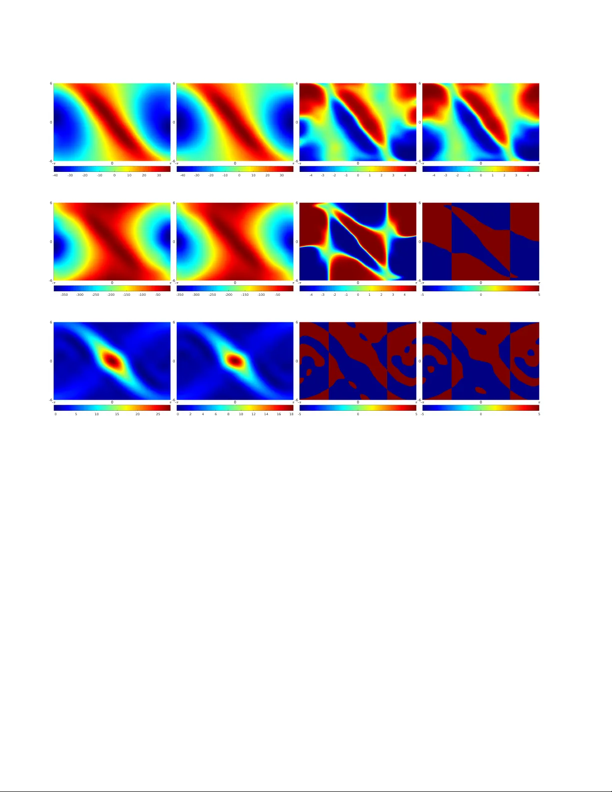
P olicy Iterations f or Reinf or cement Lear ning Pr oblems in Continuous T ime and Space — Fundamental Theory and Methods ? Jaeyoung Lee a , ∗ , Richard S. Sutton b a Department of Electrical and Computer Engineering, University of W aterloo, W aterloo, ON, Canada, N2L 3G1. b Department of Computing Science, University of Alberta, Edmonton, AB, Canada, T6G 2E8. Abstract Policy iteration (PI) is a recursi ve process of polic y e valuation and improv ement for solving an optimal decision-making/control problem, or in other words, a reinforcement learning (RL) problem. PI has also served as the fundamental for developing RL methods. In this paper , we propose two PI methods, called differential PI (DPI) and inte gral PI (IPI), and their variants, for a general RL frame work in continuous time and space (CTS), where the en vironment is modeled by a system of ordinary differential equations (ODEs). The proposed methods inherit the current ideas of PI in classical RL and optimal control and theoretically support the existing RL algorithms in CTS: TD-learning and value-gradient-based (V GB) greedy policy update. W e also provide case studies including 1) discounted RL and 2) optimal control tasks. Fundamental mathematical properties — admissibility , uniqueness of the solution to the Bellman equation (BE), monotone improv ement, con ver gence, and optimality of the solution to the Hamilton-Jacobi-Bellman equation (HJBE) — are all inv estigated in-depth and impro ved from the existing theory , along with the general and case studies. Finally , the proposed ones are simulated with an inv erted-pendulum model and their model-based and partially model-free implementations to support the theory and further inv estigate them beyond. K ey wor ds: policy iteration, reinforcement learning, optimization under uncertainties, continuous time and space, iterativ e schemes, adaptiv e systems 1 Introduction Policy iteration (PI) is a class of approximate dynamic programming (ADP) for recursi vely solving an optimal decision-making/control problem by alternating between policy evaluation to obtain the v alue function (VF) w .r .t. the current polic y (a.k.a. the current control la w in control theory) and policy impr ovement to improv e the policy by optimizing it using the obtained VF (Sutton and Barto, 2018; Puterman, 1994; Lewis and Vrabie, 2009). PI was ﬁrst proposed by How ard (1960) in a stochastic en viron- ment known as the Markov decision process (MDP) and has served as a fundamental principle for dev eloping RL methods, especially for an en vironment modeled or approx- imated by an MDP in discrete time and space. Con ver gence ? The authors gratefully ackno wledge the support of Alberta Innov ates–T echnology Futures, the Alberta Machine Intelligence Institute, DeepMind, the Natural Sciences and Engineering Re- search Council of Canada, and the Japanese Science and T echnol- ogy agency (JST) ERA TO project JPMJER1603: HASUO Meta- mathematics for Systems Design. ∗ Corresponding author. T el.: +1 587 597 8677. Email addresses: jaeyoung.lee@uwaterloo.ca (Jaeyoung Lee), rsutton@ualberta.ca (Richard S. Sutton). of such PIs towards the optimal solution has been proven, with the ﬁnite-time con ver gence for a ﬁnite MDP (Puter- man, 1994, Theorems 6.4.2 and 6.4.6); the forward-in-time computation of PI like the other ADP methods alleviates the problem known as the curse of dimensionality (Powell, 2007). A discount factor γ ∈ [0 , 1] is normally introduced to both PI and RL to suppress the future rew ard and thereby hav e a ﬁnite return. Sutton and Barto (2018) give a com- prehensiv e ov ervie w of PI and RL algorithms with their practical applications and recent success. On the other hand, the dynamics of a real physical task is in the majority of cases modeled as a system of (ordinary) differential equations (ODEs) inevitably in continuous time and space (CTS). PI has also been studied in such a contin- uous domain mainly under the framework of deterministic optimal control, where the optimal solution is characterized by the partial differential Hamilton-Jacobi-Bellman (HJB) equation (HJBE). Howe ver , an HJBE is extremely difﬁcult or hopeless to solve analytically , except for a very few ex- ceptional cases. PI methods in this ﬁeld are often referred to as successive approximations of the HJBE (for recursiv ely solving it!), and the main difference among them lies in their policy ev aluation — the earlier PI methods solve the asso- ciated differ ential Bellman equation (BE) (a.k.a. L yapunov or Hamiltonian equation) to obtain each VF for the target policy (e.g., Leake and Liu, 1967; Kleinman, 1968; Saridis and Lee, 1979; Beard, Saridis, and W en, 1997; Abu-Khalaf and Lewis, 2005 to name a few). Murray , Cox, Lendaris, and Saeks (2002) proposed a trajectory-based policy ev al- uation that can be viewed as a deterministic Monte-Carlo prediction (Sutton and Barto, 2018). Moti vated by those two approaches abov e, Vrabie and Le wis (2009) proposed a par- tially model-free 1 PI scheme called integral PI (IPI), which is more relev ant to RL in that the associated BE is of a tem- poral difference (TD) form — see Lewis and Vrabie (2009) for a comprehensiv e overvie w . Fundamental mathematical properties of those PIs, i.e., conv ergence, admissibility , and monotone improvement of the policies, are in vestigated in the literature abov e. As a result, it has been shown that the policies generated by PI methods are always monotonically improv ed and admissible; the sequence of VFs generated by PI methods in CTS is shown to con verge to the optimal solution, quadratically in the LQR case (Kleinman, 1968). These fundamental properties are discussed, improved, and generalized in this paper in a general setting that includes both RL and optimal control problems in CTS. On the other hand, the aforementioned PI methods in CTS were all designed via L yapunov’ s stability theory (Khalil, 2002) to ensure that the generated policies all asymptotically stabilizes the dynamics and yield ﬁnite returns (at least on a bounded region around an equilibrium state), provided that so is the initial policy . Here, the dynamics under the initial policy needs to be asymptotically stable to run the PI meth- ods, which is, howe ver , quite contradictory for IPI — it is partially model-free, b ut it is hard or ev en impossible to ﬁnd such a stabilizing policy without knowing the dynamics . Be- sides, compared with the RL problems in CTS, e.g., those in (Doya, 2000; Mehta and Meyn, 2009; Fr ´ emaux, Sprekeler , and Gerstner, 2013), this stability-based approach restricts the range of the discount factor γ and the class of the dy- namics and the cost (i.e., reward) as follows. (1) When discounted, the discount factor γ ∈ (0 , 1) must be larger than some threshold so as to hold the asymp- totic stability of the target optimal policy (Gaitsgory , Gr ¨ une, and Thatcher, 2015; Modares, Le wis, and Jiang, 2016). If not, there is no point in considering stability: PI ﬁnally con ver ges to that (possibly) non-stabilizing optimal solution, ev en if the PI is conv ergent and the initial policy is stabilizing . Furthermore, the threshold on γ depends on the dynamics (and the cost), and thus it cannot be calculated without knowing the dynamics, a contradiction to the use of any (partially) model-free methods such as IPI. Due to these restrictions on γ , the PI methods mentioned abov e for nonlinear optimal control focused on the problems without discount fac- tor , rather than discounted ones. (2) In the case of optimal regulations, (i) the dynamics is 1 The term “partially model-free” in this paper means that the algorithm can be implemented using some partial kno wledge (i.e., the input-coupling terms) of the dynamics f in (1). assumed to ha ve at least one equilibrium state; 2 (ii) the goal is to stabilize the system optimally for that equi- librium state, although bifurcation or multiple isolated equilibrium states to be considered may exist; (iii) for such optimal stabilization, the cost is crafted to be pos- itiv e (semi-)deﬁnite — when the equilibrium state of interest is transformed to zero without loss of general- ity (Khalil, 2002). Similar restrictions exist in optimal tracking problems that can be transformed into equiv- alent optimal regulation problems (e.g., see Modares and Le wis, 2014). In this paper, we consider a general RL framework in CTS, where reasonably minimal assumptions were imposed — 1) the global existence and uniqueness of the state trajectories, 2) (whenev er necessary) continuity , differentiability , and/or existence of maximum(s) of functions, and 3) no assump- tion on the discount factor γ ∈ (0 , 1] — to include a broad class of problems. The RL problem in this paper not only contains those in the RL literature (e.g., Doya, 2000; Mehta and Meyn, 2009; Fr ´ emaux et al., 2013) in CTS but also considers the cases be yond stability frame work (at least the- oretically), where state trajectories can be still bounded or ev en diver ge (Proposition 2.2; §5.4; Appendices §§G.2 and G.3 on pages 31–34). It also includes input-constrained and unconstrained problems presented in both RL and optimal control literature as its special cases. Independent of the research on PI, se v eral RL methods hav e been proposed in CTS based on RL ideas in the discrete do- main. Adv antage updating was proposed by Baird III (1993) and then reformulated by Doya (2000) under the en viron- ment represented by a system of ODEs; see also T allec, Blier , and Ollivier (2019)’ s recent extension of advantage updating using deep neural networks. Doya (2000) also ex- tended TD( λ ) to the CTS domain and then combined it with his proposed policy improvement methods such as the value-gradient-based (VGB) greedy policy update. See also Fr ´ emaux et al. (2013)’ s extension of Doya (2000)’ s contin- uous actor-critic with spiking neural networks. Mehta and Meyn (2009) proposed Q-learning in CTS based on stochas- tic approximation. Unlike in MDP , ho we ver , these RL meth- ods were rarely relev ant to the PI methods in CTS due to the gap between optimal control and RL — the proposed PI methods bridge this gap with a direct connection to TD learning in CTS and VGB greedy policy update (Doya, 2000; Fr ´ emaux et al., 2013). The inv estigations of the ADP for the other RL methods remain as a future work or see our preliminary result (Lee and Sutton, 2017). 1.1 Main Contributions In this paper , the main goal is to build up a theory on PI in a general RL framew ork, from the ideas of PI in classical RL and optimal control, when the time domain and the state- action space are all continuous and a system of ODEs models 2 For an example of a dynamics with no equilibrium state, see (Haddad and Chellaboina, 2008, Example 2.2). 2 the en vironment. As a result, a series of PI methods are proposed that theoretically support the existing RL methods in CTS: TD learning and VGB greedy policy update. Our main contributions are summarized as follows. (1) Motiv ated by the PI methods in optimal control, we propose a model-based PI named differential PI (DPI) and a partially model-free PI called IPI, for our general RL framework. The proposed schemes do not necessar- ily require an initial stabilizing policy to run and can be considered a sort of fundamental PI methods in CTS. (2) By case studies that contain both discounted RL and optimal control framew orks, the proposed PI methods and theory for them are simpliﬁed, improved, and spe- cialized, with strong connections to RL and optimal control in CTS. (3) Fundamental mathematical properties regarding PI (and ADP) — admissibility , uniqueness of the solution to the BE, monotone impro vement, conv ergence, and optimal- ity of the solution to the HJBE — are all inv estigated in- depth along with the general and case studies. Optimal control case studies also examine the stability properties of PI. As a result, the existing properties for PI in opti- mal control are improved and rigorously generalized. Simulation results for an inv erted-pendulum model are also provided, with the model-based and partially model-free im- plementations to support the theory and further in vestigate the proposed methods under an admissible (but not neces- sarily stabilizing) initial policy , with the strong connections to ‘bang-bang control’ and ‘RL with simple binary reward, ’ both of which are beyond the scope of our theory . Here, the RL problem in this paper is formulated stability-freely (which is well-deﬁned under the minimal assumptions), so that the (initial) admissible policy is not necessarily stabiliz- ing in the theory and the proposed PI methods for solving it. 1.2 Or ganizations This paper is organized as follows. In §2, our general RL problem in CTS is formulated along with mathematical backgrounds, notations, and statements related to BEs, pol- icy improvement, and the HJBE. In §3, we present and discuss the two main PI methods (i.e., DPI and IPI) and their variants, with strong connections to the existing RL methods in CTS. W e show in §4 the fundamental properties of the proposed PI methods: admissibility , uniqueness of the solution to the BE, monotone improvement, con ver gence, and optimality of the solution to the HJBE. Those properties in §4 and the Assumptions made in §§2 and 4 are simpliﬁed, improv ed, and relax ed in §5 with the follo wing case studies: 1 ) concav e Hamiltonian formulations (§5.1); 2 ) discounted RL with bounded VF/reward (§5.2); 3 ) RL problem with local Lipschitzness (§5.3); 4 ) nonlinear optimal control (§5.4). In §6, we discuss and provide the simulation results of the main PI methods. Finally , conclusions follow in §7. W e separately provide Appendices (see page 19 below and thereafter) that contain a summary of notations and termi- nologies (§A), related works and highlights (§B), details re- garding the theory and implementations (§§C–E, and H), a pathological e xample (§F), additional case studies (§G), and all the proofs (§I). Throughout the paper , any section start- ing with an alphabet as abov e will indicate a section in the appendices. 1.3 Notations and T erminologies The following notations and terminologies will be used throughout the paper (see §A for a complete list of notations and terminologies, including those not listed below). In any mathematical statement, iff stands for “if and only if ” and s.t. for “such that”. “ . = ” indicates the equality relationship that is true by deﬁnition . (Sets, vectors, and matrices). N and R are the sets of all natural and real numbers, respecti vely . R n × m is the set of all n -by- m real matrices. A T is the transpose of A ∈ R n × m . R n . = R n × 1 denotes the n -dimensional Euclidean space. k x k is the Euclidean norm of x ∈ R n , i.e., k x k . = ( x T x ) 1 / 2 . (Euclidean topology). Let Ω ⊆ R n . Ω is said to be compact iff it is closed and bounded. Ω o denotes the interior of Ω ; ∂ Ω is the boundary of Ω . If Ω is open, then Ω ∪ ∂ Ω (resp. Ω ) is called an n -dimensional manifold with (resp. without) boundary . A manifold contains no isolated point. (Functions, sequences, and con vergence). A function f : Ω → R m is said to be C 1 , denoted by f ∈ C 1 , iff all of its ﬁrst-order partial deriv atives exist and are continuous over the interior Ω o ; ∇ f : Ω o → R m × n denotes the gradient of f . f ( E ) . = { f ( x ) : x ∈ E } for E ⊆ Ω denotes the image of E under f . A sequence of functions h f i i ∞ i =1 , abbreviated by h f i i or f i , is said to conv erge locally uniformly iff for each x ∈ Ω , there is a neighborhood of x on which h f i i conv erges uniformly . For any two functions f 1 , f 2 : R n → [ −∞ , ∞ ) , we write f 1 6 f 2 iff f 1 ( x ) ≤ f 2 ( x ) for all x ∈ R n . 2 Preliminaries Let X . = R l be a state space and T . = [0 , ∞ ) the underlying time space. An m -dimensional manifold U ⊆ R m with or without boundary is called an action space. W e also denote X T . = R 1 × l for notational con venience. The en vironment in this paper is described in CTS by a system of ODEs: ˙ X t = f ( X t , U t ) , U t ∈ U (1) where t ∈ T is time instant, U ⊆ R m is an action space, and the dynamics f : X × U → X is a continuous function; X t , ˙ X t ∈ X denote the state vector and its time deriv ativ e, at time t , respectiv ely; the action trajectory t 7→ U t is a continuous function from T to U . W e assume that t = 0 is the initial time without loss of generality 3 and that 3 If the initial time t 0 is non-zero, then proceed with the time variable t 0 = t − t 0 , which satisﬁes t 0 = 0 at the initial time t = t 0 . 3 Assumption. The state trajectory t 7→ X t satisfying (1) is uniquely deﬁned over the entire time interval T . 4 A policy π refers to a continuous function π : X → U that determines the state trajectory t 7→ X t by U t = π ( X t ) for all t ∈ T . For notational efﬁcienc y , we employ the G - notation G x π [ Y ] , which means the value Y when X 0 = x and U t = π ( X t ) for all t ∈ T . Here, G stands for “Generator , ” and G x π can be thought of as the corresponding notation of the expectation E π [ · | S 0 = x ] in the RL literature (Sutton and Barto, 2018), without playing any stochastic role. Note that the limits and integrals are exchangeable with G x π [ · ] in order (whenev er those limits and integrals are deﬁned for any X 0 ∈ X and any action trajectory t 7→ U t ). For example, for any continuous function v : X → R , G x π  Z v ( X t ) dt  = Z G x π  v ( X t )  dt = Z v  G x π [ X t ]  dt, where the three mean the same: R v ( X t ) dt when X 0 = x and U t = π ( X t ) ∀ t ∈ T . Also note: G x π [ U t ] = G x π [ π ( X t )] . Finally , the time-deri vati ve ˙ v : X × U → R of a C 1 function v : X → R is given by ˙ v ( X t , U t ) = ∇ v ( X t ) f ( X t , U t ) — applying the chain rule and (1). Here, X t ∈ X and U t ∈ U are free v ariables, and ˙ v is continuous since so are f and ∇ v . 2.1 RL pr oblem in Continuous T ime and Space The RL problem considered in this paper is to ﬁnd the best policy π ∗ that maximizes the inﬁnite horizon value function (VF) v π : X → [ −∞ , ∞ ) deﬁned as v π ( x ) . = G x π  Z ∞ 0 γ t · R t dt  , (2) where the rew ard R t is determined by a continuous reward function r : X × U → R as R t = r ( X t , U t ) ; γ ∈ (0 , 1] is the discount factor . Throughout the paper , the attenuation rate α . = − ln γ ≥ 0 will be used interchangeably for simplicity . For a policy π , we denote f π ( x ) . = f ( x, π ( x )) and r π ( x ) . = r ( x, π ( x )) ; both are continuous as so are f , r , and π by deﬁnitions. Assumption. A maximum of the re war d function r : r max . = max  r ( x, u ) : ( x, u ) ∈ X × U  exists and for γ = 1 , r max = 0 . 5 Note that the integrand t 7→ γ t R t is continuous since so are t 7→ X t , t 7→ U t , and r . So, by the abov e assumption on r , 4 Not imposed on our problem for generality but strongly related to this Assumption is Lipschitz continuity of f and f π . See §5.3 for related discussions; for more study , see (Khalil, 2002, Section 3.1) with the system ˙ x = f 0 ( t, x ) , where f 0 ( t, x ) . = f ( x, U t ) or f π ( x ) . 5 If r max 6 = 0 and γ = 1 , then proceed with the reward function r 0 ( x, u ) . = r ( x, u ) − r max whose maximum is now zero. the time integral and thus the VF v π in (2) are well-deﬁned in the Lebesque sense (Folland, 1999, Chapter 2.3) and, as stated belo w , uniformly upper-bounded. Lemma 2.1 Ther e exists a constant v ∈ R s.t. v π 6 v for any policy π ; v = 0 for γ = 1 and otherwise, v = r max /α . By Lemma 2.1, the VF is always less than some constant, but it is still possible that v π ( x ) = −∞ for some x ∈ X . In this paper , the ﬁnite VFs are characterized by the notion of admissibility gi ven below . Deﬁnition. A policy π (or its VF v π ) is said to be admissible, denoted by π ∈ Π a (or v π ∈ V a ), iff v π ( x ) is ﬁnite for all x ∈ X . Here , Π a and V a denote the sets of all admissible policies and admissible VFs, respectively . T o make our RL problem feasible, we assume: Assumption. Ther e exists at least one admissible policy , and every admissible VF is C 1 . (3) The following proposition gi ves a criterion for admissibility and boundedness. Proposition 2.2 A policy π is admissible if ther e exist a function ξ : X → R and a constant α < α , both possibly depending on the policy π , such that ∀ x ∈ X : G x π [ R t ] ≥ ξ ( x ) · exp( α t ) for all t ∈ T . (4) Mor eover , v π is bounded if so is ξ . Remark. The criterion (4) means that the re war d R t un- der π does not diverg e to −∞ exponentially with the rate α or higher . F or γ = 1 (i.e., α = 0 ), it means exponential con ver gence R t → 0 . The condition (4) is fairly general and so satisﬁed by the examples in §§5.2, G.2, and G.3. 2.2 Bellman Equations with Boundary Condition Deﬁne the Hamiltonian function h : X × U × X T → R as h ( x, u, p ) . = r ( x, u ) + p f ( x, u ) (5) (which is continuous as so are f and r ) and the γ -discounted cumulativ e reward R η up to a given time horizon η > 0 as R η . = Z η 0 γ t · R t dt as a short-hand notation. The following lemma then shows the equi valence of the Bellman-like (in)equalities. Lemma 2.3 Let ∼ be a binary relation on R that belongs to { = , ≤ , ≥} and v : X → R be C 1 . Then, for any policy π , v ( x ) ∼ G x π  R η + γ η · v ( X η )  (6) holds for all x ∈ X and all horizon η > 0 iff α · v ( x ) ∼ h ( x, π ( x ) , ∇ v ( x )) ∀ x ∈ X . (7) 4 By splitting the time-integral in (2) at η > 0 , we can easily see that the VF v π satisﬁes the Bellman equation (BE): v π ( x ) = G x π  R η + γ η · v π ( X η )  (8) that holds for any x ∈ X and any η > 0 . Assuming v π ∈ V a and using (8), we obtain its boundary condition at η = ∞ . Proposition 2.4 Suppose that π is admissible. Then, lim t →∞ G x π  γ t · v π ( X t )  = 0 ∀ x ∈ X . By the application of Lemma 2.3 to the BE (8) under (3), the follo wing differ ential BE holds whenever π ∈ Π a : α · v π ( x ) = h ( x, π ( x ) , ∇ v π ( x )) , (9) where the function x 7→ h ( x, π ( x ) , ∇ v π ( x )) is continuous since so are the associated functions h , π , and ∇ v π . When- ev er necessary , we call (8) the integr al BE to distinguish it from the differ ential BE (9). In what follows, we state that the boundary condition (12), the counterpart of that in Proposition 2.4, is actually neces- sary and sufﬁcient for a solution v of the BE (10) or (11) to be equal to the corresponding VF v π and ensure π ∈ Π a . Theorem 2.5 (Policy Evaluation) F ix the horizon η > 0 and suppose there exists a function v : X → R s.t. either of the followings holds for a policy π : (1) v satisﬁes the integr al BE: v ( x ) = G x π  R η + γ η · v ( X η )  ∀ x ∈ X ; (10) (2) v is C 1 and satisﬁes the differ ential BE: α · v ( x ) = h ( x, π ( x ) , ∇ v ( x )) ∀ x ∈ X . (11) Then, π is admissible and v = v π iff lim k →∞ G x π  γ k · η · v ( X k · η )  = 0 ∀ x ∈ X . (12) For suf ﬁciency , the boundary condition (12) can be replaced by the conditions on v and r π (and R t ) in Theorem C.4 in §C. These conditions are particularly related to the optimal control framew ork in §5.4 but applicable to any case in this paper as an alternative to (12) (see §C for more). 2.3 P olicy Impr ovement Deﬁne a partial order among policies: π 4 π 0 iff v π 6 v π 0 . Then, we say that a policy π 0 is improved o ver π iff π 4 π 0 . In CTS, the Bellman inequality in Lemma 2.6 for v = v π ensures this policy improv ement over an admissible policy π . The inequality becomes the BE (9) when v = v π and π = π 0 . Lemma 2.6 If v ∈ C 1 is upper-bounded (by zer o if γ = 1 ) and satisﬁes for a policy π 0 α · v ( x ) ≤ h ( x, π 0 ( x ) , ∇ v ( x )) ∀ x ∈ X , then π 0 is admissible and v 6 v π 0 . In what follo ws, for the e xistence of a maximally impro ving policy , we assume on the Hamiltonian function h : Assumption. Ther e exists a function u ∗ : X × X T → U such that u ∗ is continuous and u ∗ ( x, p ) ∈ arg max u ∈U h ( x, u, p ) ∀ ( x, p ) ∈ X × X T . (13) Here, (13) simply means that for each ( x, p ) , the function u 7→ h ( x, u, p ) has its maximum at u ∗ ( x, p ) ∈ U . Then, for any admissible policy π , there exists a continuous function π 0 : X → U such that π 0 ( x ) ∈ arg max u ∈U h ( x, u, ∇ v π ( x )) ∀ x ∈ X . (14) W e call such π 0 a maximal policy (over π ∈ Π a ). Giv en u ∗ , a maximal policy π 0 can be directly obtained by π 0 ( x ) = u ∗ ( x, ∇ v π ( x )) . (15) In general, there may exist multiple maximal policies, but if u ∗ in (13) is unique , then π 0 satisfying (14) is uniquely gi ven by (15). For non-afﬁne optimal control problems, Leake and Liu (1967) and Bian, Jiang, and Jiang (2014) imposed as- sumptions similar to the above Assumption on u ∗ plus its uniqueness. Here, the e xistence of u ∗ is ensured if U is com- pact; u ∗ is unique if the function u 7→ h ( x, u, p ) is strictly concav e and C 1 for each ( x, p ) — (i) see §D for details and more; (ii) for such examples, see §5.1; Cases 1 and 2 in §6. Theorem 2.7 (Policy Improv ement) Suppose π is admissible. Then, the policy π 0 given by (14) is also admissible and satisﬁes π 4 π 0 . 2.4 Hamilton-J acobi-Bellman Equation (HJBE) Under the Assumptions made so far , the optimal solution of the RL problem can be characterized via (i) the HJBE (16): α · v ∗ ( x ) = max u ∈U h ( x, u, ∇ v ∗ ( x )) ∀ x ∈ X (16) and (ii) the associated policy π ∗ : X → U such that π ∗ ( x ) ∈ arg max u ∈U h ( x, u, ∇ v ∗ ( x )) ∀ x ∈ X , (17) both of which are the keys to prove the con ver gence of PIs tow ards the optimal solution v ∗ (and π ∗ ) in §4. Note that once a C 1 solution v ∗ : X → R to the HJBE (16) exists, then so does a continuous function (i.e., a policy) π ∗ satisfying (17), by the Assumption of the existence of a continuous function u ∗ satisfying (13), and is given by π ∗ ( x ) = u ∗ ( x, ∇ v ∗ ( x )) . (18) In what follows, we show that satisfying the HJBE (16) and (17) is necessary for ( v ∗ , π ∗ ) to be optimal ov er the entire admissible space. Theorem 2.8 If there e xists an optimal policy π ∗ whose VF v ∗ satisﬁes v 6 v ∗ for any v ∈ V a , then v ∗ and π ∗ satisfy the HJBE (16) and (17) , respectively . 5 There may e xist another optimal policy π 0 ∗ than π ∗ , b ut their VFs are always the same by π ∗ 4 π 0 ∗ and π 0 ∗ 4 π ∗ and equal to a solution v ∗ to the HJBE (16) by Theorem 2.8. In this paper , if exist, π ∗ denotes any one of the optimal policies, and v ∗ is the unique common VF for them which we call the optimal VF . In general, they denote a solution v ∗ to the HJBE (16) and an associated HJB policy π ∗ s.t. (17) holds (or an associated function π ∗ satisfying (17) that is potentially discontinuous — see §§4.1 and E.1). Remark 2.9 The re war d function r has to be appropriately designed in such a way that the function u 7→ h ( x, u, p ) for each ( x, p ) at least has a maximum (so that (13) holds for some u ∗ ). Otherwise, the maximal policy π 0 in (14) and/or the solution v ∗ to the HJBE (16) (and accor dingly , π ∗ in (17) ) may not exist since neither do the maxima in those equations. Such a pathological example is given in §F for a simple non-af ﬁne dynamics f . In §5.1.2, we r evisit this issue and pr opose a technique applicable to a class of non-afﬁne RL pr oblems to ensure the existence and continuity of u ∗ . W e note that the optimality of the HJB solution ( v ∗ , π ∗ ) is studied more in §E, e.g., the suf ﬁcient conditions and case studies, in connection with the PIs presented in §3 below . 3 Policy Iterations Now , we are ready to state our two main PI schemes, DPI and IPI. Here, the former is a model-based approach, and the latter is a partially model-free PI. Their simpliﬁed (par- tially model-free) versions discretized in time will be also discussed after that. Until §6, we present and discuss those PI schemes in an ideal sense without introducing (i) any function approximator , such as neural network, and (ii) any discretization in the state space. 6 3.1 Differ ential P olicy Iteration (DPI) Our ﬁrst PI, named differential policy iteration (DPI), is a model-based PI scheme extended from optimal control to our RL framew ork (e.g., see Leake and Liu, 1967; Beard et al., 1997; Abu-Khalaf and Lewis, 2005). Algorithm 1 describes the whole procedure of DPI — it starts with an initial admissible policy π 0 (line 1) and performs policy ev aluation and improv ement until v i and/or π i con ver ges (lines 2–5). In policy evaluation (line 3), the agent solves the differential BE (19) to obtain the VF v i = v π i − 1 for the last policy π i − 1 . Then, v i is used in policy impr ovement (line 4) so as to obtain the next policy π i by maximizing the associated Hamiltonian function in (20). Here, if v i = v ∗ , then π i = π ∗ by (17) and (20). 6 When we implement any of the PI schemes, both are obviously required (except linear quadratic re gulation (LQR) cases) since the structure of the VF is veiled and it is impossible to perform the policy ev aluation and improvement for an (uncountably) inﬁnite number of points in the continuous state space X (see also §6 for implementation examples, with §H for details). Algorithm 1: Differential Policy Iteration (DPI) 1 Initialize: ( π 0 , an initial admissible policy; i ← 1 , iteration index; 2 repeat 3 Policy Evaluation: given π i − 1 , ﬁnd a C 1 function v i : X → R satisfying the differential BE: α · v i ( x ) = h ( x, π i − 1 ( x ) , ∇ v i ( x )) ∀ x ∈ X ; (19) 4 Policy Improv ement: ﬁnd a policy π i such that π i ( x ) ∈ arg max u ∈U h ( x, u, ∇ v i ( x )) ∀ x ∈ X ; (20) 5 i ← i + 1 ; until con ver gence is met. Basically , DPI is model-based (see the deﬁnition (5) of h ) and does not rely on any state trajectory data. On the other hand, its policy ev aluation is closely related to TD learning methods in CTS (Doya, 2000; Fr ´ emaux et al., 2013). T o see this, note that (19) can be expressed w .r .t. ( X t , U t ) as G x π i − 1 [ δ t ( v i )] = 0 for all x ∈ X and t ∈ T , where δ t denotes the TD error deﬁned as δ t ( v ) . = R t + ˙ v ( X t , U t ) − α · v ( X t ) for any C 1 function v : X → R . Fr ´ emaux et al. (2013) used δ t ( v ) as the TD error in their model-free actor-critic and approximated v and the model-dependent part ˙ v of δ t ( v ) by a spiking neural network. δ t ( v ) is also the TD error in TD(0) in CTS (Doya, 2000), where ˙ v ( X t , U t ) is approximated by ( v ( X t ) − v ( X t − ∆ t )) / ∆ t in backward time, for a sufﬁciently small time step ∆ t chosen in the interval (0 , α − 1 ) ; under this backward-in-time approximation, δ t ( v ) can be expressed in a similar form to the TD error in discrete-time as δ t ( v ) ≈ R t + ˆ γ d · V ( X t ) − V ( X t − ∆ t ) (21) for V . = v / ∆ t and ˆ γ d . = 1 − α ∆ t ≈ e − α ∆ t ( = γ ∆ t ). Here, the discount factor ˆ γ d belongs to (0 , 1) if so is γ , thanks to ∆ t ∈ (0 , α − 1 ) , and ˆ γ d = 1 whenev er γ = 1 . In summary , policy ev aluation of DPI solves the differential BE (19) that idealizes the existing TD learning methods in CTS (Doya, 2000; Fr ´ emaux et al., 2013). 3.2 Inte gral P olicy Iteration (IPI) Algorithm 2 describes the second PI, integral policy iteration (IPI), whose difference from DPI is that (19) and (20) for the policy ev aluation and improvement are replaced by (22) and (23), respectively . The other steps are the same as DPI, except that the time horizon η > 0 is initialized (line 1) before the main loop. In policy evaluation (line 3), IPI solves the integral BE (22) for a giv en ﬁxed horizon η > 0 without using the explicit knowledge of the dynamics f of the system (1) — there are no explicit terms of f in (22), and the information on 6 Algorithm 2: Integral Policy Iteration (IPI) 1 Initialize:      π 0 , an initial admissible policy; η > 0 , time horizon; i ← 1 , iteration index; 2 repeat 3 Policy Evaluation: given π i − 1 , ﬁnd a C 1 function v i : X → R satisfying the integral BE: v i ( x ) = G x π i − 1  R η + γ η · v i ( X η )  ∀ x ∈ X ; (22) 4 Policy Improv ement: ﬁnd a policy π i such that π i ( x ) ∈ arg max u ∈U  r ( x, u ) + ∇ v i ( x ) f c ( x, u )  ∀ x ∈ X ; (23) 5 i ← i + 1 ; until con ver gence is met. the dynamics f is implicitly captured by the state trajectory data { X t : 0 ≤ t ≤ η } generated under π i − 1 at each of the i th iteration, for a number of initial states X 0 ∈ X . Note that by Theorem 2.5, solving the integral BE (22) for a ﬁxed η > 0 and its differential version (19) in DPI are equiv alent (as long as v i satisﬁes the boundary condition (28) in §4). In policy impro vement (line 4), we consider the decomposi- tion (24) of the dynamics f : f ( x, u ) = f d ( x ) + f c ( x, u ) , (24) where f d : X → X called a drift dynamics is independent of the action u and assumed unknown , and f c : X × U → X is the corresponding input-coupling dynamics assumed known a priori ; 7 both f d and f c are assumed continuous. Since the term ∇ v π ( x ) f d ( x ) does not contribute to the maximization with respect to u , policy improvement (14) can be rewritten under the decomposition (24) as π 0 ( x ) ∈ arg max u ∈U  r ( x, u ) + ∇ v π ( x ) f c ( x, u )  ∀ x ∈ X (25) by which the policy improvement (line 4) of Algorithm 2 is directly obtained. Note that the policy improvement (23) in Algorithm 2 and (25) are partially model-free — the maxi- mizations do not depend on the unknown drift dynamics f d . The policy e valuation and improv ement of IPI are com- pletely and partially model-free, respectiv ely . Thus the whole procedure of Algorithm 2 is partially model-free, i.e., it can be done ev en when a drift dynamics f d is completely unknown. In addition to this partially model-free nature, the horizon η > 0 in IPI can be any value — it can be large or small — as long as the cumulativ e rew ard R η has no signiﬁcant error when approximated in practice. In this sense, the time horizon η plays a similar role as the num- ber n in the n -step TD predictions in discrete-time (Sutton 7 There are an inﬁnite number of ways of choosing f d and f c ; one typical choice is f d ( x ) = f ( x, 0) and f c ( x, u ) = f ( x, u ) − f d ( x ) . and Barto, 2018). Indeed, if η = n ∆ t for some n ∈ N and a sufﬁciently small ∆ t > 0 , then by the forward-in-time approximation R η ≈ G n · ∆ t , where G n . = R 0 + γ d · R ∆ t + γ 2 d · R 2∆ t + · · · + γ n − 1 d · R ( n − 1)∆ t and γ d . = γ ∆ t ∈ (0 , 1] , the integral BE (22) is expressed as V i ( x ) ≈ G x π i − 1  G n + γ n d · V i ( X η )  , (26) where V i . = v i / ∆ t . W e can also apply a higher-order ap- proximation of R η — for instance, under the trapezoidal approximation, we have V i ( x ) ≈ G x π i − 1 h G n + 1 2 · ( γ n d · R η − R 0 ) + γ n d · V i ( X η ) i , which employs the end-point reward R η while (26) does not. Note that the TD error (21) is not easy to generalize for such multi-step TD predictions. When n = 1 , on the other hand, the n -step BE (26) becomes V i ( x ) ≈ G x π i − 1  R 0 + γ d · V i ( X ∆ t )  ∀ x ∈ X , (27) which is similar to the BE in discrete-time (Sutton and Barto, 2018) and G x π [ δ t ( v )] ≈ 0 for the TD error (21) in CTS. 3.3 V ariants with T ime Discr etizations As discussed in §§3.1 and 3.2 above, the BEs in DPI and IPI can be discretized in time in order to (1) approximate ˙ v i = ∇ v i · f in DPI, model-freely; (2) calculate the cumulativ e rew ard R η in IPI; (3) yield TD formulas similar to the BEs in discrete-time. For instance, for a sufﬁciently small ∆ t , the discretized BE corresponding to DPI and TD(0) in CTS (Doya, 2000) is: V π ( x ) ≈ G x π  R ∆ t + ˆ γ d · V π ( X ∆ t )  ∀ x ∈ X , where V π . = v π / ∆ t . The discretized BE for IPI is ob viously of the form (27) for n = 1 and (26) for n > 1 (or one of the BEs with a higher-order approximation of R η ). If the integral BE (8) is discretized with the trapezoidal approximation for n = 1 , then we also hav e V π ( x ) ≈ G x π h 1 2 · ( R 0 + γ d · R ∆ t ) + γ d · V π ( X ∆ t ) i ∀ x ∈ X . Combining any one of those BEs, discretized in time, with the follo wing policy improvement: π 0 ( x ) ∈ arg max u ∈U  r ( x, u ) + ∆ t · ∇ V π ( x ) f c ( x, u )  ∀ x ∈ X , where ∆ t · ∇ V π replaces ∇ v π in (25), we can further obtain a partially model-free variant of the proposed PI methods. For example, a one-step IPI v ariant ( n = 1 ) is sho wn in §5.2 (when the reward or initial VF is bounded). These variants are practically important since they contain neither ˙ v i nor ˙ V i (both of which depend on the full-dynamics f ) nor the cumulativ e reward R η (which has been approximated out in the variants of IPI). As these variants are approximate 7 versions of DPI and IPI, they also approximately satisfy the same properties as DPI and IPI shown in the subsequent sections. 4 Fundamental Properties of Policy Iterations This section shows the fundamental properties of DPI and IPI — admissibility , the uniqueness of the solution to each policy ev aluation, monotone impro vement, and con ver gence (tow ards an HJB solution). W e also discuss the optimality of the HJB solution (§§4.2 and E.1) based on the con ver gence properties of PIs. In any mathematical statements, h v i i and h π i i denote the sequences of the solutions to the BEs and the policies, both generated by Algorithm 1 or 2 under: Boundary Condition. If π i − 1 is admissible, then lim t →∞ G x π i − 1  γ t · v i ( X t )  = 0 ∀ x ∈ X . (28) Theorem 4.1 π i − 1 is admissible and v i = v π i − 1 ∀ i ∈ N . Mor eover , the policies ar e monotonically impr oved, that is, π 0 4 π 1 4 · · · 4 π i − 1 4 π i 4 · · · . Theorem 4.2 (Con vergence) Denote ˆ v ∗ ( x ) . = sup i ∈ N v i ( x ) . Then, ˆ v ∗ is lower semicontinuous; v i → ˆ v ∗ a. pointwise; b . uniformly on Ω ⊂ X if Ω is compact and ˆ v ∗ is continuous over Ω ; c. locally uniformly if ˆ v ∗ is continuous. In what follows, ˆ v ∗ always denotes the con ver ging function ˆ v ∗ ( x ) . = sup i ∈ N v i ( x ) = lim i →∞ v i ( x ) in Theorem 4.2. 4.1 Con ver gence towar ds v ∗ and π ∗ Now , we provide con ver gence v i → v ∗ to a solution v ∗ of the HJBE (16). One core technique is to use the PI operator T : V a → V a deﬁned on the space V a of admissible VFs as ( T v π i − 1 . = v π i for any i ∈ N ; T v π . = v π 0 for any other v π ∈ V a , where π 0 is a maximal policy over the giv en policy π ∈ Π a . Let T N be the N th recursion of T deﬁned as T 0 v . = v and T N v . = T N − 1 ( T v ) for v ∈ V a . Then, the VF sequence h v i i satisﬁes v i = T i − 1 v 1 for all i ∈ N . In what follows, we denote v ∗ a (unique) ﬁxed point of T . Proposition 4.3 If v ∗ is a ﬁxed point of T , then v ∗ = v ∗ , i.e., v ∗ is a solution v ∗ to the HJBE (16) . By Proposition 4.3, conv ergence v i → v ∗ implies that h v i i con ver ges towards a solution v ∗ to the HJBE (16). In what follows, we ﬁrst show the conv ergence v i → v ∗ under: Assumption 4.4 T has a unique ﬁxed point v ∗ . Theorem 4.5 Under Assumption 4.4, ther e exists a metric d : V a × V a → [0 , ∞ ) such that T is a contraction (and thus continuous) under d and v i → v ∗ in the metric d . Theorem 4.5 shows the con ver gence v i → v ∗ in a metric d under which T is continuous. Howe ver , there is no informa- tion about which metric it is. In what follows, we focus on locally uniform con ver gence, in connection to Theorem 4.2. Let d Ω be a pseudometric on V a deﬁned for Ω ⊆ X as d Ω ( v , w ) . = sup    v ( x ) − w ( x )   : x ∈ Ω  for v , w ∈ V a . Then, uniform con vergence v i → v ∗ on Ω becomes equiv a- lent to conv ergence v i → v ∗ in the pseudometric d Ω . Theorem 4.6 Suppose ˆ v ∗ ∈ V a and for each compact subset Ω of X , T is continuous under d Ω . If Assumption 4.4 is true, then v i → v ∗ locally uniformly and v ∗ = ˆ v ∗ . The conv ergence condition in Theorem 4.6 comes from Leake and Liu (1967)’ s approach that is now extended to our RL framew ork. The next theorem is motiv ated by the con ver gence results of PIs for optimal control of input-af ﬁne dynamics (Saridis and Lee, 1979; Beard et al., 1997; Mur- ray et al., 2002; Abu-Khalaf and Lewis, 2005; Vrabie and Lewis, 2009) and provides the conditions for stronger con- ver gence tow ards v ∗ and π ∗ . Assumption 4.7 F or each x ∈ X , the argmax -corr espondence p 7→ arg max u ∈U h ( x, u, p ) has a closed graph. That is, for each x ∈ X and any sequence h p k i in X T con ver ging to p ∗ ,    u k ∈ arg max u ∈U h ( x, u, p k ) lim k →∞ u k = u ∗ ∈ U = ⇒ u ∗ ∈ arg max u ∈U h ( x, u, p ∗ ) . Assumption 4.8 ( a. h∇ v i i con ver ges locally uniformly; b . h π i i con ver ges pointwise. Theorem 4.9 Under Assumptions 4.7 and 4.8, ˆ v ∗ is a solu- tion v ∗ to the HJBE (16) such that v ∗ ∈ C 1 and (1) v i → v ∗ , ∇ v i → ∇ v ∗ both locally uniformly; (2) π i → π ∗ pointwise, for a function π ∗ satisfying (17) . Remark 4.10 If the argmax -set is a singleton (so the max- imal function u ∗ satisfying (13) is unique), then Assump- tion 4.7 is equivalent to continuity of p 7→ u ∗ ( x, p ) for each x ∈ X and thus implied by the continuity of u ∗ assumed in §2.3! In this particular case, π ∗ in Theorem 4.9 is uniquely given by (18) hence continuous (i.e., π ∗ satisﬁes our deﬁni- tion of a policy). F or such examples, see §§5.1.1 and G.3. In summary , we hav e established the follo wing con ver gence properties: ( C 1 ) con ver gence v i → v ∗ in a metric; ( C 2 ) locally uniform con ver gence v i → v ∗ ; ( C 3 ) locally uniform con ver gence ∇ v i → ∇ v ∗ , and pointwise con ver gence π i → π ∗ , 8 under certain conditions and the minimal assumptions made in this section and §2. (W eak/Strong Con vergence) Theorem 4.5 ensures weak con ver gence ( C 1 ) under Assumption 4.4 only . Theorem 4.6 giv es strong conv ergence ( C 2 ), provided that the following additional conditions hold: (i) continuity of T in the uniform pseudometric d Ω ; (ii) the con vergence within the admissible space V a : lim i →∞ v i ∈ V a , i.e., ˆ v ∗ ∈ V a . W e note that (1) the unique ﬁxed point v ∗ therein and in Assumption 4.4 is a solution v ∗ to the HJBE (16) (Proposition 4.3); (2) whenev er ( C 2 ) is true, both v ∗ and v ∗ therein are char- acterized by Theorem 4.2 as v ∗ = v ∗ = ˆ v ∗ . (Stronger Con vergence) If the con vergence described in Assumptions 4.7 and 4.8 are all true, then Theorem 4.9 en- sures the stronger conv ergence properties ( C 2 ) and ( C 3 ) for v ∗ = ˆ v ∗ ∈ C 1 , wherein the limit function ˆ v ∗ ( = lim i →∞ v i ) becomes a solution v ∗ to the HJBE (16). In this case, (1) T is ne ver used, hence no assumption is imposed on T ; (2) π ∗ in ( C 3 ) is not necessarily a policy by our deﬁnition due to its possible discontinuity (see also Remark 4.10); (3) the concave Hamiltonian formulation in §5.1 ensures π i → π ∗ locally uniformly for a policy π ∗ , with both Assumptions 4.7 and 4.8b r elaxed (e.g., Theorem 5.1). 4.2 Optimality of the HJB Solution: Sufﬁcient Conditions For each type of con ver gence above, we provide a suf ﬁcient condition for v ∗ in the HJBE (16) to be optimal in the sense that for any given initial admissible policy π 0 , v i → v ∗ in the respectiv e manner with monotonicity v i 6 v i +1 ∀ i ∈ N . For the optimality of v ∗ with the stronger con vergence, ( C 2 ) and ( C 3 ), we additionally assume that: Assumption 4.11 The solution v ∗ to the HJBE (16) , if ex- ists, is unique over C 1 and upper-bounded (by zer o if γ = 1 ). Those sufﬁcient conditions for optimality and related dis- cussions are presented in Appendix §E.1. 5 Case Studies W ith strong connections to RL and optimal control in CTS, this section studies the special cases of the general RL prob- lem formulated in §2. In those case studies, the proposed PI methods and theory for them are simpliﬁed and improv ed as summarized in T able 1. The blanks in T able 1 are ﬁlled with “ Assumed” or, in simpliﬁed policy improvement sec- tions, “No”. The connections to stability theory in optimal control are also made in this section. The optimality of the HJB solution ( v ∗ , π ∗ ) for each case is studied and summa- rized in §E.2; more case studies are given in §G. For simplicity , we let f x ( u ) . = f ( x, u ) and r x ( u ) . = r ( x, u ) for x ∈ X . Both f x and r x are continuous for each x since so are f and r . The mathematical terminologies employed in this section are given in §A, with a summary of notations. 5.1 Concave Hamiltonian F ormulations Here, we study the special settings of the reward function r , which make the function u 7→ h ( x, u, p ) strictly concave and C 1 (after some input-transformation in the cases of non- afﬁne dynamics). In these cases, policy improvement maxi- mizations (13), (14), and (17) become conv ex optimizations whose solutions exist and are gi v en in closed-forms. W e will see that this dramatically simpliﬁes the policy improvement itself and strengthen the con ver gence properties. Although we focus on certain classes of dynamics — the input-afﬁne and then a class of non-afﬁne ones — the idea is extendible to a general nonlinear system of the form (1) (see §G.1 for such an extension). 5.1.1 Case I: Input-afﬁne Dynamics First, consider the following case: for each x ∈ X , (1) f x is af ﬁne , i.e., the input-coupling term f c ( x, u ) in the decomposition (24) is linear in u , so that the dynamics f can be represented as f ( x, u ) = f d ( x ) + F c ( x ) u (29) for a matrix-valued continuous function F c : X → R l × m ; (2) r x is strictly concave and repr esented by r ( x, u ) = r ( x ) − c ( u ) (30) where r : X → R is continuous, c : U → R is strictly con ve x and C 1 , and its gradient ∇ c is surjective , i.e., ∇ c ( U o ) = R 1 × m . Here, U o is the interior of U . This framework includes those in (Rekasius, 1964; Beard et al., 1997; Doya, 2000; Abu-Khalaf and Le wis, 2005; Vra- bie and Lewis, 2009; Lee, Park, and Choi, 2015) as spe- cial cases; it still contains a broad class of dynamics such as Newtonian dynamics (e.g., robot manipulator and ve- hicle models). In this case, the mapping u 7→ h ( x, u, p ) is strictly concave and C 1 (see the deﬁnition (5) of h ). Hence, as mentioned in §2.3 (see §D for the behind the- ory), the unique maximal function u ∗ ≡ u ∗ ( x, p ) satisfying (13) corresponds to the unique regular point ¯ u ∈ U ◦ s.t. −∇ c ( ¯ u ) + p F c ( x ) = 0 , where the gradient ∇ c T : U o → R m is strictly monotone and bijectiv e on its domain U o (see §I.3). Rearranging it w .r .t. ¯ u , we obtain the closed-form so- lution u ∗ of (13): u ∗ ( x, p ) = σ  F T c ( x ) p T  , (31) where σ . = ( ∇ c T ) − 1 denotes the in verse of ∇ c T . Here, the mapping σ : R m → U o is also strictly monotone and continuous (see §I.3); thus, u ∗ is continuous. Substituting (31) into (15), we obtain the unique closed-form solution of the policy improvement maximization (14) (or (25)): π 0 ( x ) = σ  F T c ( x ) ∇ v T π ( x )  (32) a.k.a. the value-gradient-based (VGB) greedy policy update (Doya, 2000). This simpliﬁes the policy improvement of DPI and IPI (and their variants) shown in §3 as 9 T able 1 Summary of Case Studies: Relaxations and Simpliﬁcations of the Assumptions and Policy Improvement Problem Formulation Concav e Hamiltonian Discounted RL with bounded RL with local Lipschitzness (b) Nonlinear optimal control (b) LQR VF (a) state trj. Section 5.1 / G.1 5.2 G.2 5.3 5.4 G.3 Global existence and uniqueness of state trjs. T rue, conditionally (c) T rue Existence of an admissible policy , i.e., V a 6 = ∅ T rue C 1 -regularity (3) and continuity of admissible VFs Continuous, conditionally (b) Assumptions 4.4 and 4.11 (w .r .t. T and the HJBE) Existence of a continuous maximal function u ∗ T rue Boundary conditions (12) and (28) T rue, conditionally (d) T rue T rue, conditionally (e) Assumptions 4.7 and 4.8 for ( C2 ) and ( C3 ) Relaxed (f ) Simpliﬁed policy improvement Y es Y es (a) Once the initial VF v π 0 in the PI methods is bounded, so is v π i for all i ∈ N ; a stronger case is when the reward function r is bounded. (b) f and/or f π is assumed locally Lipschitz. (c) T rue if f π is locally Lipschitz in §G.2 and in addition, in §§5.3 and 5.4, if π ∈ Π a (see the modiﬁed deﬁnitions of Π a therein). (d) T rue if v and v i are bounded — this makes sense only when the target VF is bounded. (e) See Theorems 5.16 (attracti veness and asymptotic stability) and 5.17 (conditions in Theorem C.4 of §C), both for (12). See also Theorem 5.19 for (28). (f ) Assumptions 4.7 and 4.8 are reduced to Assumption 4.8a (see Theorems 4.9, 5.1, and 5.4). Policy Improv ement: update the next policy π i by π i ( x ) = σ  F T c ( x ) ∇ v T i ( x )  . Similarly , the HJB policy π ∗ satisfying (17) is also uniquely giv en by (18) and (31), i.e., π ∗ ( x ) = σ  F T c ( x ) ∇ v T ∗ ( x )  , un- der (29) and (30). Moreover , Theorem 4.9 can be simpliﬁed and strengthened, with Assumptions 4.7 and 4.8b relaxed . Theorem 5.1 Under (29) , (30) , and Assumption 4.8a, ˆ v ∗ is a solution v ∗ to the HJBE (16) such that v ∗ ∈ C 1 and v i → v ∗ , ∇ v i → ∇ v ∗ , and π i → π ∗ , all locally uniformly . Remark 5.2 Assumption 4.8a is necessary for con ver gence in Theorem 5.1 and, in fact so ar e similar uniform conver - gence assumptions on h∇ v i i for conver gence given in the existing literatur e on PIs for optimal contr ol (e.g., Saridis and Lee, 1979; Bear d et al., 1997; Murray , Cox, and Saeks, 2003; Abu-Khalaf and Lewis, 2005; Bian et al., 2014 to name a few). This is due to the fact that even the uniform con ver gence of v i (e.g ., Theorem 4.2c) implies nothing about the con ver gence of its gradient ∇ v i ; it cannot even ensure the differ entiability of the limit function ˆ v ∗ (Rudin, 1964; Thomson, Bruckner , and Bruckner, 2001). Her e, Assump- tion 4.8a or any type of (uniform) conver gence of h∇ v i i is by no means trivial to pr ove, and thus its r elaxation r emains as a future work (even in the optimal contr ol frameworks in the existing literatur e, which are similar to that in §5.4 under (29) – (30) , to the best authors’ knowledge). One way to effecti vely take the input constraints into con- siderations is to construct the action space U as U =  u ∈ R m : | u j | ≤ u max ,j , 1 ≤ j ≤ m  , where u j ∈ R is the j th element of u , and u max ,j ∈ (0 , ∞ ] is the corresponding physical constraint. In this case, c in (30) can be chosen as c ( u ) = lim v → u Z v 0 ( s T ) − 1 ( u ) · Γ d u (33) for a positiv e deﬁnite matrix Γ ∈ R m × m and a continuous function s : R m → U o that is strictly monotone, odd, and bijectiv e and makes c ( u ) in (33) ﬁnite at any point u on the boundary ∂ U ; 8 This formulation giv es a closed-form expression σ ( u ) = ( ∇ c T ) − 1 ( u ) = s (Γ − 1 u ) and includes the sigmoidal examples (Cases 1 and 2) in §6 as special cases — see also (Doya, 2000; Abu-Khalaf and Lewis, 2005) for similar sigmoidal examples. Another well-known example is the unconstrained problem: U = R m ( u max ,j = ∞ for each j ) and s ( u ) = u / 2 , (34) by which (33) becomes c ( u ) = u T Γ u ; the LQR case in §G.3 with E = 0 shows such an example. Remark 5.3 Once r x is strictly concave for each x ∈ X , the r ewar d function r can be always repr esented as r ( x, u ) = r ( x ) − c ( x, u ) , (35) wher e r and c ar e continuous; c x . = c ( x, · ) for each x ∈ X is strictly conve x. In this general case, if c x is C 1 and its gradient ∇ c x is surjective for each x ∈ X , then the unique maximal function u ∗ and policy π 0 over π ∈ Π a can be obtained in the same way to (31) and (32) as ( u ∗ ( x, p ) = σ x  F T c ( x ) p T  π 0 ( x ) = σ x  F T c ( x ) ∇ v T π ( x )  8 ∂ U = { u ∈ R m : u j = u max ,j for some j = 1 , 2 , · · · , m } . 10 for the inver se σ x of ( ∇ c x ) T . In addition, if ( x, u ) 7→ σ x ( u ) is continuous, then Theorem 5.1 (speciﬁcally , Lemma I.7 in §I.3) can be generalized with σ r eplaced by σ x . Some examples of such σ x ar e as follows. (1) Γ in (33) is a continuous function over X . In this case, σ x is given by σ x ( u ) = s (Γ − 1 ( x ) · u ) . (2) In the LQR setting (§G.3), σ x ( u ) = Γ − 1 ( u / 2 − E T x ) and whenever E = 0 , σ x ( u ) = σ ( u ) = Γ − 1 u / 2 . 5.1.2 Case II: a Class of Non-afﬁne Dynamics If f x is not afﬁne, then the choice of the reward function r is critical. Provided in §F is such an example, where a choice of r in the form of (30) and (33) fails to giv e closed-form solutions to policy improvement and the HJBE (16). More- ov er , in the unconstrained case, such a choice of r may result in a pathological Hamiltonian h as shown in §F . Such pathological behavior and dif ﬁculty , on the other hand, can be avoided for the non-afﬁne dynamics f of the form: f ( x, u ) = f d ( x ) + F c ( x ) ϕ ( u ) , (36) where ϕ : U → A ⊆ R m is a continuous function from the action space U to another action space A and has its in verse ϕ − 1 : A o → U o between the interiors. Note that (36) corresponds to the decomposition (24) with the input- coupling part f c ( x, u ) = F c ( x ) ϕ ( u ) and includes the input- afﬁne dynamics (29) as a special case ϕ ( u ) = u and A = U . Motiv ated by Kiumarsi, Kang, and Lewis (2016), we propose to set the reward function r under (36) as r ( x, u ) = r ( x ) − c ( ϕ ( u )) , (37) where r : X → R and c : A → R are functions that satisfy the properties of r and c in (30) but w .r .t. the action space A in place of U . Under (36) and (37), the proposed PIs ha ve the following properties, e xtended from §5.1.1 (e.g., from Theo- rem 5.1), although the argmax-set “ arg max u ∈U h ( x, u, p ) ” in this case may not be a singleton (another maximizer may exist on the boundary ∂ U ). Theorem 5.4 Let ˜ σ ( u ) . = ϕ − 1 [ σ ( u )] . Under (36) and (37) , a. a maximal policy π 0 over π ∈ Π a is explicitly given by π 0 ( x ) = ˜ σ  F T c ( x ) ∇ v T π ( x )  ; b . if the policies ar e updated in policy impro vement by π i ( x ) = ˜ σ  F T c ( x ) ∇ v T i ( x )  , then under Assumption 4.8a, ˆ v ∗ is a solution v ∗ to the HJBE (16) s.t. v ∗ ∈ C 1 and v i → v ∗ , ∇ v i → ∇ v ∗ , and π i → π ∗ , all locally uniformly , wher e π ∗ ( x ) = ˜ σ  F T c ( x ) ∇ v T ∗ ( x )  . Similarly to Remark 5.3, the results are extendible to the general case where ϕ and/or c depends on the state x ∈ X . 5.2 Discounted RL with Bounded VF Boundedness of a VF is stronger than admissibility . Like- wise, when discounted, a bounded VF can have stronger properties and statements than admissible ones. One exam- ple is continuity in the ne xt proposition; the extension to the general cases ( γ = 1 and/or v π ∈ V a ) is by no means tri vial. Proposition 5.5 Suppose that f π is locally Lipschitz and that γ ∈ (0 , 1) . Then, v π is continuous if v π is bounded. Continuity is a necessary condition to be C 1 . In the RL prob- lem formulation in §2, we have assumed the C 1 -regularity (3) and thereby continuity on every admissible VF , but no proof was provided regarding them; Proposition 5.5 above bridges this gap when the VF is discounted and bounded. In this case, the boundary condition (12) is also true as follows. Proposition 5.6 If v : X → R is bounded and γ ∈ (0 , 1) , then v satisﬁes the boundary condition (12) for any policy π . Moreov er , when the VF is discounted and bounded, the BE (10) (resp. (11)) has the unique solution v = v π ov er all bounded (resp. bounded C 1 ) functions, and the boundedness is preserved under the policy improvement operation. Corollary 5.7 Let γ ∈ (0 , 1) and π be a policy . Then, (1) if there exists a bounded function v satisfying the inte- gral BE (10) or with v ∈ C 1 , the differ ential BE (11) , then v π is bounded (hence, admissible) and v = v π . (2) if v π is bounded (hence, admissible), then so is v π 0 and we have π 4 π 0 , where π 0 is a maximal policy over π . In fact, if the reward function r is bounded, then so is the VF for any giv en policy (so long as the state trajectory t 7→ X t exists); hence the above results become stronger as follows. Assumption 5.8 r is bounded and γ ∈ (0 , 1) . Corollary 5.9 Under Assumption 5.8, the followings hold for any given policy π and any maximal policy π 0 over π : (1) v π and v π 0 ar e bounded (hence, admissible); π 4 π 0 ; (2) v π is continuous if f π is locally Lipschitz; (3) if a bounded function v satisﬁes the inte gral BE (10) or with v ∈ C 1 , the differ ential BE (11) , then v = v π . For a given policy π , the VF properties in Corollary 5.9 are also true when γ ∈ (0 , 1) and r π (but not necessarily r ) is bounded (see and slightly modify the proof of Corollary 5.9 in §I.3). In this case (and the general cases where γ ∈ (0 , 1) , and v π is bounded somehow), Proposition 5.5, Corollary 5.7, and mathematical induction show that T N v π for any N ∈ N satisﬁes the properties of the VFs in Corollary 5.9. In other words, if for the initial policy π 0 , Assumption. r π 0 (or the VF v π 0 ) is bounded and γ ∈ (0 , 1) 11 which is weaker than Assumption 5.8, then the sequences h v i i and h π i i generated by DPI or IPI satisfy: for any i ∈ N , (1) v i = v π i − 1 , (2) v π i − 1 is bounded and π i − 1 4 π i , (3) v π i − 1 is continuous if f π i − 1 is locally Lipschitz, under the boundedness of each v i to ensure the boundary condition (28) to be true by Proposition 5.6. Algorithm 3: V ariants of IPI and DPI with Bounded v π 0 1 Initialize:      π 0 , an initial policy s.t. v π 0 is bounded; ∆ t > 0 , a small time step ( 0 < ∆ t  1 ); i ← 1 ; 2 repeat (under γ ∈ (0 , 1) ) 3 Policy Evaluation: given policy π i − 1 , ﬁnd a bounded C 1 function V i : X → R such that for all x ∈ X , (IPI V ariant): V i ( x ) ≈ G x π i − 1  R 0 + γ d · V i ( X ∆ t )  ; (DPI V ariant): for α d . = α ∆ t ( = − ln γ d ), α d · V i ( x ) = h  x, π i − 1 ( x ) , ∆ t · ∇ V i ( x )  ; 4 Policy Improv ement: ﬁnd a policy π i s.t. for all x ∈ X , π i ( x ) ∈ arg max u ∈U  r ( x, u ) + ∆ t · ∇ V i ( x ) f c ( x, u )  ; 5 i ← i + 1 ; until con ver gence is met. Algorithm 3 shows the respectiv e variants of IPI and DPI when γ ∈ (0 , 1) and the VF v π 0 w .r .t. the initial policy π 0 is bounded. Here, the boundedness of v π 0 can be made by that of r or r π 0 . In policy ev aluation, the variants of IPI and DPI solve, for V i . = v i / ∆ t , the discretized BE (27) and the dif ferential BE (19), respecti vely; the other steps of both variants are the same and derived from their originals (Al- gorithms 1 and 2) by replacing η and v i with the small time step ∆ t and ∆ t · V i , respectiv ely . Implementation examples of both variants in Algorithm 3 are giv en and discussed in §6 with sev eral types of (bounded) rew ard functions r and a function approximator for V i . The other types of variants (e.g., IPI with the n -step prediction (26)) can be also ob- tained by replacing the BE in policy ev aluation with one of the other BEs in §3 (e.g., (26)). Since these variants all as- sume both γ ∈ (0 , 1) and the boundedness of the initial VF v π 0 , it is sufﬁcient to ﬁnd a bounded C 1 function V i in each policy e valuation (line 3) for holding the properties abov e regarding h v i i and h π i i without assuming the boundary con- dition (28) on v i ( = ∆ t · V i ). 5.3 RL with Local Lipschitzness Let ( Π Lip . = the set of all locally Lipschitz policies, C 1 Lip . = { v ∈ C 1 : ∇ v is locally Lipschitz } . In §§5.3 and 5.4, we consider the RL problems, where Assumption. The dynamics f and the maximal function u ∗ in (13) are locally Lipschitz, and always use the notations π 0 and π ∗ to denote the maximal and HJB policies given by (15) and (18), respectively . The Assumption implies continuity of f and u ∗ and ensures: (1) π 0 and π ∗ are locally Lipschitz (i.e., π 0 , π ∗ ∈ Π Lip ) so long as v π in (15) and v ∗ in (18) are C 1 Lip , respectiv ely; (2) the dynamics f π under π ∈ Π Lip is locally Lipschitz, and thereby the state trajectory t 7→ G x π [ X t ] for each x ∈ X is uniquely deﬁned and C 1 ov er the maximal existence interval [0 , t max ( x ; π )) ⊆ T (see Khalil, 2002, Section 3.1 and Theorem 3.1 therein). Here, t max ( x ; π ) ∈ (0 , ∞ ] is deﬁned for and depends on both initial state x and π ∈ Π Lip ; whene ver t max ( x ; π ) < ∞ , G x π ( k X t k ) → ∞ as t → t max ( x ; π ) . T o circumvent this ﬁnite-time explosion issue, we set v π ( x ) to “ −∞ ” whene ver t max ( x ; π ) is ﬁnite, that is, redeﬁne v π as v π ( x ) . =      G x π  Z ∞ 0 γ t · R t dt  if t max ( x ; π ) = ∞ , −∞ , otherwise. (38) Here, existence and uniqueness of the state trajectories were not assumed; t max ( · ; π ) and thus v π in (38) are well-deﬁned as long as π ∈ Π Lip . Hence, with slight ab use of notation, we restrict the admissible sets Π a and V a by redeﬁning them as Π a . = { π ∈ Π Lip : v π ( x ) is ﬁnite for all x ∈ X } , V a . = { v π : π ∈ Π a } . Note that for each x ∈ X , the value v π ( x ) is ﬁnite and the state trajectory t 7→ G x π [ X t ] is deﬁned uniquely and C 1 ov er the entire time interval T if π ∈ Π a (or equiv alently , if v π ∈ V a ). Here, the global existence of the unique state trajectories was assumed in the general RL problem formulated in §2 but now is encapsulated by admissibility . In what follows, we provide the policy improv ement theorem extended from Theorem 2.7, without assuming any existence and uniqueness of the state trajectories, but under Assumption. V a ⊂ C 1 Lip to ensure the maximal policy π 0 ∈ Π Lip whenev er π ∈ Π a . Theorem 5.10 (Policy Improv ement) If there e xist a com- pact subset Ω ⊂ X and K ∞ functions ρ 1 , ρ 2 such that for a policy π ∈ Π a , ρ 1 ( k x k Ω ) ≤ v − v π ( x ) ≤ ρ 2 ( k x k Ω ) ∀ x ∈ X , wher e k x k Ω . = inf y ∈ Ω k x − y k , then π 0 ∈ Π a and π 4 π 0 . 12 5.4 Nonlinear Optimal Control The objective of optimal control is to stabilize the system (1) w .r .t. a given equilibrium point ( x e , u e ) while minimizing a giv en cost functional. Here, any point in X × U such that ˙ x e = f ( x e , u e ) ≡ 0 is called an equilibrium point ( x e , u e ) ; it can be transformed to (0 , 0) and thus let ( x e , u e ) = (0 , 0) without loss of generality (Khalil, 2002) and assume that f (0 , 0) = 0 . Note that if a policy π satisﬁes π (0) = 0 , then we hav e 0 = f π (0) , i.e., x e = 0 is an equilibrium point of the system (1) under π . The optimal control frame work in this subsection is a partic- ular case of the locally Lipschitz RL problem in §5.3 abo ve. Hence, we impose the same assumptions on it: the local Lip- schitzness of f and u ∗ , with π 0 and π ∗ denoting the respec- tiv e policies given by (15) and (18), the inclusion V a ⊂ C 1 Lip , and the extended deﬁnition (38) of the VF v π for π ∈ Π Lip . On the other hand, we deﬁne a class of policies Π 0 as Π 0 . = { π ∈ Π Lip : π (0) = 0 } and, with slight abuse of notation, redeﬁne Π a and V a by Π a . = { π ∈ Π 0 : v π ( x ) is ﬁnite for all x ∈ X } and V a . = { v π : π ∈ Π a } . Here, we have merely added the condition π (0) = 0 into the deﬁnitions of Π a and V a in §5.3. W ith these notations, x e = 0 comes to be an equilibrium point of the system (1) under π ∈ Π 0 ( ⊇ Π a ). Similarly to §5.3, this subsection does not assume existence and uniqueness of the state trajectories; π ∈ Π a (or v π ∈ V a ) ensures: for e very x ∈ X , the state trajectory t 7→ G x π [ X t ] is uniquely deﬁned and C 1 ov er T . In addition, the boundary conditions (12) and (28) are not assumed but either proven to be true or replaced by their sufﬁcient ones shown in §C (e.g., see Theorem 5.17). Whenev er necessary , we use the cost functions c . = − r and c π . = − r π , the cost VF J π . = − v π , and J ∗ . = − v ∗ , rather than − r , − r π , − v π , and − v ∗ , respectiv ely , for simplicity and consistency to optimal control conv entions; the cost at time t ∈ T is denoted by C t . = c ( X t , U t ) = − R t . W e consider a positiv e deﬁnite cost function c , i.e., assume c ( x, u ) > 0 ∀ ( x, u ) 6 = (0 , 0) , and c (0 , 0) = 0 . (39) Then, by (39) and the deﬁnition, the value J π ( x ) is always restricted to [0 , ∞ ] and, similarly to (38), J π ( x ) = ∞ when- ev er t max ( x ; π ) < ∞ ; otherwise, J π ( x ) = G x π  R ∞ 0 γ t C t dt  . Lemma 5.11 c π for π ∈ Π 0 is positive deﬁnite. Lemma 5.12 Let π ∈ Π a . Then, a. J π is positive deﬁnite; b . x 7→ ˙ J π ( x, π ( x )) is negative semideﬁnite iff αJ π 6 c π (40) and c. x 7→ ˙ J π ( x, π ( x )) is negative deﬁnite iff αJ π ( x ) < c π ( x ) ∀ x ∈ X \ { 0 } . (41) In what follows, we assume that c π for any π ∈ Π 0 is radially non v anishing 9 (§A.4). Giv en the conditions in Lemma 5.12, J π is, in fact, a L yapuno v function (Khalil, 2002) for the system ˙ X t = f π ( X t ) as shown in the following theorem. Theorem 5.13 The equilibrium point x e = 0 of dynamics f π under π ∈ Π a is stable if (40) holds, asymptotically stable if (41) is true, and globally asymptotically stable if γ = 1 or , in addition to (41) , J π is radially unbounded. Remark 5.14 Whenever γ = 1 , (i) (41) is true since α = 0 and c π is positive deﬁnite by Lemma 5.11; (ii) admissibility dir ectly implies global asymptotic stability by Theorem 5.13 (her e, the radial unboundedness of J π is not assumed!). Next, we show global attractiveness (hence, global asymp- totic stability) ensures uniqueness of the solution to the BEs. Deﬁnition 5.15 x e is globally attractive under π iff t max ( x ; π ) = ∞ and lim t →∞ G x π [ X t ] = x e ∀ x ∈ X . Theorem 5.16 (Policy Evaluation) Let x e = 0 under π ∈ Π 0 be globally attractive . If there exists a function v : X → R s.t. v is continuous at 0 , v (0) = 0 , and the BE (10) or , with v ∈ C 1 , the BE (11) holds, then π ∈ Π a and v = v π . The uniqueness of the solution to the BE can be also giv en under other conditions. When discounted, it has a more gen- eral condition than both (40) and (41) for stability as well as contains the cases where x e = 0 is not necessarily (globally) attractiv e, and the state trajectories could even div erge. Theorem 5.17 (Policy Evaluation) Let J ( . = v ) be positive deﬁnite and κ · J 6 c π for a policy π ∈ Π 0 and a constant κ > 0 . Then, π ∈ Π a and v = v π if either of a or b below is true. a. v is C 1 , radially unbounded, and satisﬁes the BE (11) or alternatively , the BE (10) for arbitrary small η > 0 ; b . v satisﬁes the BE (10) for a ﬁxed η > 0 , c π is radially unbounded, and there exist a function ζ : X → R and α < α , possibly depending on π , s.t. for each x ∈ X , G x π [ C t ] ≤ ζ ( x ) exp( α t ) ∀ t ∈ [0 , t max ( x ; π )) . (42) The policy improv ement theorem in §5.3, i.e., Theorem 5.10, can be also extended as follows. Theorem 5.18 (Policy Improv ement) Let π ∈ Π a and J π is radially unbounded. Then π 0 ∈ Π a and J π 0 6 J π . From the theory and discussions above, we propose the fol- lowing three conditions for the PI methods in the optimal control frame work: for all i ∈ N and J i . = − v i , 9 This assumption excludes any function c π such that as r → ∞ , inf k x k≥ r c π ( x ) → 0 (e.g., c π ( x ) = x 2 exp ( − x 2 ) ) and is used in Theorem 5.13 for proving global asymptotic stability for γ = 1 . 13 (A) π 0 ∈ Π a , (B) J i ∈ C 1 Lip is positi ve deﬁnite and radially unbounded, (C) if γ 6 = 1 , ( x e = 0 under π i − 1 is globally attractive, or there exists κ i > 0 s.t. κ i · J i 6 c π i − 1 . Those three conditions are devised in order to run PI (for IPI, together with (D) or (E) below), without assuming the existence of unique state trajectories and the boundary con- dition (28). Here, (C) is imposed only when γ 6 = 1 ( α > 0 ), in which case, if κ i < α , then the inequality in (C) is weak er than both of the stability conditions α J i 6 c π i − 1 and αJ i ( x ) < c π i − 1 ( x ) ∀ x 6 = X \ { 0 } (43) that correspond to (40) and (41), respectively . For running IPI under discounting γ ∈ (0 , 1) , we impose an additional condition on each π i − 1 : (D) if γ 6 = 1 , then a. c π i − 1 is radially unbounded; b. there are α i ∈ [0 , α ) and a function ζ i s.t. (42) holds ∀ x ∈ X . Here, (D a ) is true if x 7→ c ( x, u ) is radially unbounded; (D b ) is true for any policy π i − 1 that makes ev ery state tra- jectory bounded or ev en div erge exponentially with the rate smaller than α . For instance, if x e = 0 under π i − 1 is glob- ally attractiv e (so that (C) is true) or state trajectories are globally bounded, then (D b ) is always valid with α i = 0 and ζ i ( x ) = inf t ∈ T G x π i − 1 [ C t ] < ∞ , where ζ i ( x ) is ﬁnite by boundedness of t 7→ G x π [ X t ] and continuity of both c and t 7→ G x π [ X t ] . Another condition for discounted IPI that can replace the condition (D) is (E) if γ 6 = 1 , the BE (22) holds for arbitrary small η > 0 . In practice, it is impossible to solv e the BE (22) for inﬁnitely many η ’ s; one best practice for (E) is to implement IPI with one sufﬁciently small η > 0 . W e also note that when γ = 1 , (C) – (E) become irrelev ant — in this case, only (A) and (B) are required to run both IPI and DPI. Theorem 5.19 Under (A) – (C) (for IPI, with (D) or (E) ), (1) π i − 1 ∈ Π a and J i = J π i − 1 > J π i for all i ∈ N ; (2) x e = 0 under π i − 1 is globally asymptotically stable (hence, globally attractive) if (43) is true (or if γ = 1 ). W ithout assuming the boundary condition (28) and existence of unique state trajectories, the other properties in §4 can be also extended under the above conditions (A) – (C) (for IPI, together with (D) or (E) ), by following the same proofs in §4, b ut with Theorem 4.1 therein replaced by Theorem 5.19. Note that the radial unboundedness of J i in (B) makes sense only when J π i − 1 or the optimal cost VF J ∗ is radially un- bounded. For the latter case, it is guaranteed that J π for e very π ∈ Π a is radially unbounded by optimality 0 6 J ∗ 6 J π . Limitations also exist. First, it is difﬁcult to check (C) – (E) and that J π i − 1 is radially unbounded; J ∗ is unknown until we hav e found at the end. Secondly , the results cannot be applied to the locally admissible cases, where the VF (equiv alently J π ) is ﬁnite only around the equilibrium point x e = 0 locally , not globally over X . Lastly , not easy to verify in general is the local Lipschitzness assumptions on u ∗ and ∇ J π which are necessary for π 0 ∈ Π Lip . An example that is free from these limitations is the LQR (see §G.3). Remark 5.20 This article is the ﬁrst to deﬁne admissibility without asymptotic stability to the best authors’ knowledge. This concept can be broadly applied, e.g., to the discounted LQR cases in §G.3 where the system may not be stable un- der an admissible policy due to γ ∈ (0 , 1) . In fact, when γ = 1 , admissibility of a policy π (i.e., π ∈ Π a ) implies global asymptotic stability under π , with J π served as a L ya- puon v function, as discussed in Remark 5.14. This re veals that asymptotic stability can be excluded fr om the deﬁnition of admissibility , even in the existing optimal contr ol frame- works (as long as the VF is C 1 ). W e also believe that our concept of admissibility can be generalized even when v π (or equivalently , J π ) is locally ﬁnite around the equilibrium x e = 0 (i.e., locally admissible), not globally . Remark. If the dynamics f is non-afﬁne , then the cost func- tion c has to be properly designed (e.g ., by the techniques intr oduced in §§5.1.2 and G.1) to avoid the pathological Hamiltonian discussed in Remark 2.9 and §5.1.2. Note that as shown in §F , such a pathological phenomenon can hap- pen even when c is positive deﬁnite (and quadratic when unconstrained), which is a typical choice in optimal contr ol. 6 In verted-P endulum Simulation Examples T o support the theory and further in vestigate the proposed PI methods, we simulate the variants of DPI and IPI shown in Algorithm 3 applied to an inv erted-pendulum model: ¨ ϑ t = − 0 . 01 ˙ ϑ t + 9 . 8 sin ϑ t − U t cos ϑ t , where ϑ t ∈ R and U t ∈ U are the angular position of and the external torque input to the pendulum at time t , respectiv ely; the action space is given by U = [ − u max , u max ] ⊂ R , with the torque limit u max = 5 [N · m]. Letting X t . = [ ϑ t ˙ ϑ t ] T , then the dynamics can be expressed as (1) and (29) with f d ( x ) =  x 2 9 . 8 sin x 1 − 0 . 01 x 2  and F c ( x ) =  0 − cos x 1  , where x = [ x 1 x 2 ] T ∈ X ( = R 2 ). In the simulations, we set the discount factor γ = 0 . 1 and the time step ∆ t = 10 [ms]; the zero initial policy π 0 ( x ) ≡ 0 is employed. The solution V i of the policy ev aluation at each iteration i is represented by a linear function approximator V as V i ( x ) ≈ V ( x ; θ i ) . = θ T i φ ( x ) , (44) 14 (a) Case 1: concave Hamiltonian with bounded reward — DPI (b) Case 2: optimal control — DPI (c) Case 1: concave Hamiltonian with bounded reward —IPI (d) Case 3: bang-bang control — IPI with r ( x, u ) = cos x 1 (e) Case 4: bang-bang control with binary reward – DPI (f) Case 4: bang-bang control with binary reward – IPI Fig. 1. The trajectories of the pendulum angular -position ϑ t generated by the policies obtained during and after the PIs for each case study . All of the trajectories start from X 0 = ( π , 0) , and the yello w re gions correspond to those ϑ t -trajectories at iterations i = (3) , 4 , 5 , · · · , 49 . for its weights θ i ∈ R L and features φ : X → R L , with L = 121 . Each policy ev aluation determines θ i by the least- squares solution θ ∗ i minimizing the Bellman errors over the set of initial states uniformly distributed as the ( N × M )-grid points over the region Ω = [ − π , π ] × [ − 6 , 6] ⊂ X . Here, N and M are the total numbers of the grids in the x 1 - and x 2 - directions, respecti vely; we choose N = 20 and M = 21 , so the total 420 number of grid points in Ω are used as initial states. When inputting to V , the ﬁrst component x 1 of x is normalized to a value within [ − π , π ] by adding ± 2 π k to it for some k ∈ Z . In what follows, we simulate four different settings, whose learning objective is to swing up and eventually settle down the pendulum at the upright position θ t = 2 π k for some k ∈ Z , under the torque limit | U t | ≤ u max . For each case, we basically consider the reward function r giv en by (30) and (33) with s ( u ) = u max tanh( u /u max ) . (45) As the inv erted pendulum dynamics is input-afﬁne, this set- ting corresponds to the concave Hamiltonian formulation in §5.1.1 (with a bounded r if r is bounded). The implementa- tion details (the features φ , policy e valuation, and policy im- prov ement) are provided in §H; the MA TLAB/Octav e source code for the simulations is also available online. 10 6.1 Case 1: Concave Hamiltonian with Bounded Rewar d First, we consider the reward function r given by (30) and (33) with s ( · ) giv en by (45), Γ = 10 − 2 , and r ( x ) = cos x 1 . As mentioned above, this setting corresponds to the concav e Hamiltonian formulation in §5.1, resulting in the following policy improvement update rule (see §H for details): π i ( x ) ≈ π ( x ; θ ∗ i ) = − 5 tanh  cos x 1 · ∇ x 2 φ ( x ) · θ ∗ i / 5  . (46) As r (hence r ) is bounded, this setting also corresponds to “discounted RL under Assumption 5.8” in §5.2. Therefore, the initial and subsequent VFs in PIs are all bounded; the properties in §§5.1.1 and 5.2 are all true; the Assumptions in T able 1 w .r .t. §§5.1.1 and 5.2 are also all relaxed. Figs. 1(a), (c) and Figs. 2(a)–(d) show the trajectories of ϑ t under the policies obtained during PI and the estimates of the optimal solution ( v ∗ , π ∗ ) ﬁnally obtained at the iteration i = 50 , respecti vely; the yello w re gions in Fig. 1 correspond to the trajectories of ϑ t generated by the intermediate poli- 10 github .com/JaeyoungLee-UoA/PIs-for -RL-Problems-in-CTS/ 15 (a) ˆ V 50 in Case 1 — DPI (b) ˆ V 50 in Case 1 — IPI (c) ˆ π 50 in Case 1 — DPI (d) ˆ π 50 in Case 1 — IPI (e) ˆ V 50 in Case 2 — DPI (f) ˆ V 50 in Case 3 — IPI w/ (47) (g) ˆ π 50 in Case 2 — DPI (h) ˆ π 50 in Case 3 — IPI w/ (47) (i) ˆ V 50 in Case 4 — DPI (j) ˆ V 50 in Case 4 — IPI (k) ˆ π 50 in Case 4 — DPI ( ` ) ˆ π 50 in Case 4 — IPI Fig. 2. The optimal value function ˆ V 50 ( x ) = V ( x ; θ ∗ i ) | i =50 (left sides) and the optimal policy ˆ π 50 ( x ) = π ( x ; θ ∗ i ) | i =50 (right sides), estimated by DPI and IPI variants ov er Ω . The horizontal and vertical axes correspond to x 1 ( = ϑ ) and x 2 ( = ˙ ϑ ), respectively . cies obtained by the PIs at iterations i = (3) , 4 , 5 , · · · , 49 . Although both DPI and IPI variants generate rather dif ferent trajectories of ϑ t in Figs. 1(a), (c), due to the difference in the estimates of the VF and policy (e.g., see Figs. 2(a)–(d)), both methods hav e achiev ed the learning objective merely after the ﬁrst iteration. Here, the difference in the ϑ t -trajectories mainly comes from the dif ferent initial behaviors near ϑ = π — see the differences in the policies in Figs. 2(c), (d) (and also the VF estimates in Figs. 2(a), (b)) near the borderlines ϑ = ± π . Also note that both DPI and IPI methods have achiev ed our learning objectiv e without using an initial sta- bilizing policy that is usually required in the optimal control setting under the total discounting γ = 1 (e.g., Abu-Khalaf and Le wis, 2005; Vrabie and Le wis, 2009; Lee et al., 2015). 6.2 Case 2: Optimal Control A better performance can be obtained if the state rew ard function r in Case 1 is replaced by r ( x ) = − x 2 1 −  · x 2 2 with  = 10 − 2 . This setting corresponds to the nonlinear optimal control in- troduced and discussed in §5.4. In this case, whenev er input to r , the ﬁrst component x 1 is normalized to a value within [ − π , π ] . Here, r is still not bounded due to the existence of the term −  · x 2 2 , but Algorithm 3 (without assuming the boundedness of v π 0 ) can be successfully applied as shown in Figs. 1(b), 2(e), and 2(g). Fig. 1(b) illustrates the trajec- tories of ϑ t under the policies obtained by the DPI variant. Compared with Case 1, this setting giv es a better initial and asymptotic performance — every trajectory of ϑ t in Fig. 1(b) is almost the same as the ﬁnal one (f aster con vergence of the PI) and con ver ges to the goal state x = (0 , 0) more rapidly than any trajectories of ϑ t in Case 1. In particular , the initial behavior near ϑ = ± π has been improv ed, so that the poli- cies in this case swing up the pendulum much faster than Case 1. One possible explanation about this is that the higher magnitude of the gradient of r near x 1 = ± π expedites the initial swing-up process (note, in Case 1, ∇ r ( ± π , x 2 ) = 0 for any x 2 ). See also the difference of the ﬁnal VF and pol- icy in Figs. 2(e), (g) (Case 2) from those in Figs. 2(a)–(d) (Case 1). The results for IPI are almost similar to DPI in this case, so their ﬁgures are omitted. 16 6.3 Case 3: Bang-bang Control If Γ → 0 , the reward function r and the policy update rule (46) in Case 1 (§6.1) are simpliﬁed to r ( x, u ) = cos x 1 and π i ( x ) ≈ π ( x ; θ ∗ i ) = − 5 · sign  cos x 1 · ∇ x 2 φ ( x ) · θ ∗ i  (see §H for details), a bang-bang type discrete control. The PI methods can be also applied to optimize this bang-bang type controller . Note that this case is be yond our scope of the theory dev eloped in §§2–5 since the policy is discrete, not continuous. F or this bang-bang control frame work, Fig. 1(d) shows the ϑ t -trajectories under the discrete policies obtained by the IPI v ariant in Algorithm 3. Though the fast switching behavior of the control U t is inevitable near x = (0 , 0) , due to sign( · ) , the initial and asymptotic control performance, compared with Case 1, has been increased in the limit Γ → 0 up to the performance of optimal control (Case 2). By limiting Γ → 0 , the control policy in Case 2 can be also made a bang-bang type control, but in this case, with r ( x, u ) = − x 2 1 −  · x 2 2 with  = 10 − 2 . (47) W e have observed that the performance of the PI methods in this case is almost same as that shown in Fig. 1(d) for the previous case “ r ( x, u ) = cos x 1 ”, deriv ed from Case 1. Figs. 2(f) and (h) show the env elopes of the VF and the bang- bang policy under (47), both of which are consistent with the en velopes for Γ = 10 − 2 shown in Figs. 2(e) and (g). 6.4 Case 4: Bang-bang Control with Binary Rewar d In RL problems, the re ward is often binary and sparely giv en only at or near the goal state. T o inv estigate this case, we also consider the bang-bang policy given in the previous subsection, but with the binary rew ard function: r ( x, u ) = ( 1 , if | x 1 | ≤ 6 /π and | x 2 | ≤ 1 / 2 0 , otherwise, This giv es the rew ard signal R t = 1 near the goal state x = (0 , 0) only . Figs. 1(e) and (f) illustrate the θ t -trajectories under the policies generated by the DPI and IPI variants (i.e., Algorithm 3), respectiv ely . Though the initial perfor- mance is neither stable ( i = 1 ) nor consistent to each other ( i = 1 , 2 ), both PI methods eventually con v erge to the same seemingly near-optimal point ( i = 3 , 4 , · · · , 50 ). Note that the performance after learning ( i = 50 ) for both cases is the same as that of Cases 2 and 3 until around t = 3[ s ] as can be seen from Figs. 1(b) and (d)–(f). Figs. 2(i)–( ` ) also show the estimates of the optimal VF and policy at i = 50 . Although the details are a bit different, we can see that both meth- ods ﬁnally result in similar consistent estimates of the VF and policy . In this binary reward case, the shapes of the VF shown in Figs. 2(i) and (j) are distinguished from the oth- ers illustrated in Figs. 2(a),(b),(e), and (f) due to the reward information condensed near the goal state x = (0 , 0) only . Even in this situation, our PI methods were able to achiev e the goal at the end, as sho wn in Figs. 1(e) and (f). For the DPI variant, we have simulated this case with M = 20 , in- stead of M = 21 . 6.5 Discussions W e hav e simulated the v ariants of DPI and IPI (Algorithm 3) under the four scenarios above. Some of them ha ve achieved the learning objectiv e immediately at the ﬁrst iteration, and in all of the simulations, the proposed methods were able to achiev e the goal, ev entually . On the other hand, the imple- mentations of the PIs have the following issues. (1) The least-squares solution θ ∗ i of each policy ev aluation minimizes the Bellman error over a ﬁnite number of initial states in Ω (as detailed in §H), meaning that it is not the optimal choice to minimize the Bellman error ov er the entire region Ω . As mentioned in §3, the ideal policy e valuation cannot be implemented precisely— ev en when Ω is compact, it is a continuous space and thus contains an (uncountably) inﬁnite number of points that we cannot fully cover in practice. (2) As the dimension of the data matrix in the least squares is L × ( N M ) = 121 × 420 (see §H), calculating the least-squares solution θ ∗ i is computationally expensiv e, and the numerical error (and thus the conv ergence) is sensiti ve to the choice of the parameters such as (the number of) the features φ , the time step ∆ t , dis- counting factor γ , and of course, N and M . In our experiments, we have observed that Case 2 (optimal control) was least sensitiv e to those parameters. (3) The VF parameterization. Since the pendulum is sym- metric at x 1 = 0 , the VFs and policies obtained in Fig 2 are all symmetric, and thus it might be sufﬁcient to approximate the VF over [0 , π ] × [ − 6 , 6] ⊂ Ω , with a less number of weights, and use the symmetry of the problem. Due to the over -parameterization, we hav e observed that the weight vector θ ∗ i in certain situations nev er con ver ges but oscillates between tw o values, ev en after the VF V i has almost conv erged over Ω . All of these algorithmic and practical issues are beyond the scope of this paper and remain as a future work. 7 Conclusions In this paper, we proposed fundamental PI schemes called DPI (model-based) and IPI (partially model-free) to solve the general RL problem formulated in CTS. W e pro ved their fundamental mathematical properties: admissibility , unique- ness of the solution to the BE, monotone improvement, con- ver gence, and the optimality of the solution to the HJBE. Strong connections to the RL methods in CTS—TD learning and VGB greedy policy update—were made by providing the proposed ones as their ideal PIs. Case studies simpliﬁed and improv ed the proposed PI methods and the theory for them, with strong connections to RL and optimal control in 17 CTS. Numerical simulations were conducted with model- based and partially model-free implementations to support the theory and further in vestigate the proposed PI methods beyond, under an initial policy that is admissible but not stable. Unlike the existing PI methods in the stability-based framew orks, an initial stabilizing policy is not necessarily required to run the proposed ones. W e believ e that this w ork provides the theoretical background, intuition, and improv e- ment to both (i) PI methods in optimal control and (ii) RL methods, to be dev eloped in the future and dev eloped so far in CTS domain. References Abu-Khalaf, M. and Lewis, F . L. Nearly optimal control laws for nonlinear systems with saturating actuators using a neural network HJB approach. Automatica , 41(5):779–791, 2005. Baird III, L. C. Advantage updating. T echnical report, DTIC Document, 1993. Beard, R. W ., Saridis, G. N., and W en, J. T . Galerkin approxi- mations of the generalized Hamilton-Jacobi-Bellman equation. Automatica , 33(12):2159–2177, 1997. Bian, T ., Jiang, Y ., and Jiang, Z.-P . Adaptiv e dynamic program- ming and optimal control of nonlinear nonafﬁne systems. Au- tomatica , 50(10):2624–2632, 2014. Doya, K. Reinforcement learning in continuous time and space. Neural computation , 12(1):219–245, 2000. Folland, G. B. Real analysis: modern techniques and their appli- cations . John Wile y & Sons, 1999. Fr ´ emaux, N., Sprekeler, H., and Gerstner , W . Reinforcement learn- ing using a continuous time actor -critic framew ork with spiking neurons. PLoS Comput. Biol. , 9(4):e1003024, 2013. Gaitsgory , V ., Gr ¨ une, L., and Thatcher , N. Stabilization with discounted optimal control. Syst. Contr ol Lett. , 82:91–98, 2015. Haddad, W . M. and Chellaboina, V . Nonlinear dynamical systems and contr ol: a Lyapunov-based appr oach . Princeton Uni versity Press, 2008. How ard, R. A. Dynamic dro gramming and Markov processes . T ech. Press of MIT and John W iley & Sons Inc., 1960. Khalil, H. K. Nonlinear systems . Prentice Hall, 2002. Kiumarsi, B., Kang, W ., and Lewis, F . L. H ∞ control of non- afﬁne aerial systems using off-polic y reinforcement learning. Unmanned Systems , 4(01):51–60, 2016. Kleinman, D. On an iterati ve technique for Riccati equation com- putations. IEEE T rans. Autom. Cont. , 13(1):114–115, 1968. Leake, R. J. and Liu, R.-W . Construction of suboptimal control sequences. SIAM Journal on Control , 5(1):54–63, 1967. Lee, J. Y . and Sutton, R. Policy iteration for discounted rein- forcement learning problems in continuous time and space. In Pr oc. the Multi-disciplinary Conf. Reinfor cement Learning and Decision Making (RLDM) , 2017. Lee, J. Y ., Park, J. B., and Choi, Y . H. Integral reinforcement learning for continuous-time input-afﬁne nonlinear systems with simultaneous inv ariant explorations. IEEE T rans. Neural Net- works and Learning Systems , 26(5):916–932, 2015. Lewis, F . L. and Vrabie, D. Reinforcement learning and adaptiv e dynamic programming for feedback control. IEEE Circuits and Systems Magazine , 9(3):32–50, 2009. Mehta, P . and Meyn, S. Q-learning and pontryagin’s minimum principle. In Pr oc. IEEE Int. Conf. Decision and Contr ol, held jointly with the Chinese Contr ol Confer ence (CDC/CCC) , pages 3598–3605, 2009. Modares, H., Lewis, F . L., and Jiang, Z.-P . Optimal output- feedback control of unknown continuous-time linear systems using off-polic y reinforcement learning. IEEE T rans. Cybern. , 46(11):2401–2410, 2016. Modares, H. and Lewis, F . L. Linear quadratic tracking control of partially-unknown continuous-time systems using reinforce- ment learning. IEEE T ransactions on Automatic Contr ol , 59 (11):3051–3056, 2014. Murray , J. J., Cox, C. J., Lendaris, G. G., and Saeks, R. Adaptive dynamic programming. IEEE T rans. Syst. Man Cybern. P art C-Appl. Rev . , 32(2):140–153, 2002. Murray , J. J., Cox, C. J., and Saeks, R. E. The adaptiv e dynamic programming theorem. In Stability and Control of Dynamical Systems with Applications , pages 379–394. Springer, 2003. Powell, W . B. Appr oximate dynamic pr ogramming: solving the curses of dimensionality . W iley-Interscience, 2007. Puterman, M. L. Markov decision pr ocesses: discrete stochastic dynamic progr amming . John Wile y & Sons, 1994. Rekasius, Z. Suboptimal design of intentionally nonlinear con- trollers. IEEE T ransactions on Automatic Contr ol , 9(4):380– 386, 1964. Rudin, W . Principles of mathematical analysis , v olume 3. McGraw-hill New Y ork, 1964. Saridis, G. N. and Lee, C. S. G. An approximation theory of optimal control for trainable manipulators. IEEE Tr ans. Syst. Man Cybern. , 9(3):152–159, 1979. Sutton, R. S. and Barto, A. G. Reinfor cement learning: an intr o- duction . Second Edition, MIT Press, Cambridge, MA (av ailable at http://incompleteideas.net/book/the-book.html), 2018. T allec, C., Blier , L., and Ollivier , Y . Making deep Q-learning methods robust to time discretization. In International Confer- ence on Machine Learning (ICML) , pages 6096–6104, 2019. Thomson, B. S., Bruckner, J. B., and Bruckner, A. M. Elementary r eal analysis . Prentice Hall, 2001. Vrabie, D. and Lewis, F . L. Neural network approach to continuous-time direct adapti ve optimal control for partially un- known nonlinear systems. Neural Netw . , 22(3):237–246, 2009. 18 P olicy Iterations f or Reinf or cement Lear ning Problems in Continuous T ime and Space — Fundamental Theory and Methods: Appendices Jaeyoung Lee, a Richard S. Sutton b a Department of Electrical and Computer Eng., University of W aterloo, W aterloo, ON, Canada, N2L 3G1 (jaeyoung.lee@uwaterloo.ca) b Department of Computing Science, University of Alberta, Edmonton, AB, Canada, T6G 2E8 (rsutton@ualberta.ca) Abstract This supplementary document provides additional studies and all the details of the contents presented by Lee and Sutton (2020), as listed below . Roughly speaking, we present related works, details of the theory , algorithms, and implementations, additional case studies, and all the proofs, with the same abbreviations, terminologies, and notations. All the numbers of equations, sections, theorems, lemmas, etc. that do not contain any alphabet will refer to those in the main paper (Lee and Sutton, 2020), whereas any numbers starting with an alphabet correspond to those in the Appendices herein. A Notations and T erminologies . . . . . . . . . . . . . . . . . . . . . . . . . . . . . . . . . . . . . . . . . . . . 20 A.1 Abbreviations . . . . . . . . . . . . . . . . . . . . . . . . . . . . . . . . . . . . . . . . . . . . . . . . . . 20 A.2 Sets, V ectors, and Matrices . . . . . . . . . . . . . . . . . . . . . . . . . . . . . . . . . . . . . . . . . . . 20 A.3 Euclidean T opology . . . . . . . . . . . . . . . . . . . . . . . . . . . . . . . . . . . . . . . . . . . . . . . 20 A.4 Functions, Sequences, and Conv ergence . . . . . . . . . . . . . . . . . . . . . . . . . . . . . . . . . . . . 20 A.5 Reinforcement Learning . . . . . . . . . . . . . . . . . . . . . . . . . . . . . . . . . . . . . . . . . . . . 21 A.6 Policy Iteration . . . . . . . . . . . . . . . . . . . . . . . . . . . . . . . . . . . . . . . . . . . . . . . . . 21 A.7 Optimal Control and LQRs . . . . . . . . . . . . . . . . . . . . . . . . . . . . . . . . . . . . . . . . . . . 21 B Highlights and Related W orks . . . . . . . . . . . . . . . . . . . . . . . . . . . . . . . . . . . . . . . . . . . 22 C More on the Bellman Equations with the Boundary Condition . . . . . . . . . . . . . . . . . . . . . . . . . 23 D Existence and Uniqueness of the Maximal Function u ∗ . . . . . . . . . . . . . . . . . . . . . . . . . . . . . 25 E Theory of Optimality . . . . . . . . . . . . . . . . . . . . . . . . . . . . . . . . . . . . . . . . . . . . . . . . 25 E.1 Sufﬁcient Conditions for Optimality . . . . . . . . . . . . . . . . . . . . . . . . . . . . . . . . . . . . . . 26 E.2 Case Studies of Optimality . . . . . . . . . . . . . . . . . . . . . . . . . . . . . . . . . . . . . . . . . . . 28 F A Pathological Example (Kiumarsi et al., 2016) . . . . . . . . . . . . . . . . . . . . . . . . . . . . . . . . . 30 G Additional Case Studies . . . . . . . . . . . . . . . . . . . . . . . . . . . . . . . . . . . . . . . . . . . . . . . 30 G.1 General Concav e Hamiltonian Formulation . . . . . . . . . . . . . . . . . . . . . . . . . . . . . . . . . . 30 G.2 Discounted RL with Bounded State Trajectories . . . . . . . . . . . . . . . . . . . . . . . . . . . . . . . 31 G.3 Linear Quadratic Regulations (LQRs) . . . . . . . . . . . . . . . . . . . . . . . . . . . . . . . . . . . . . 32 H Implementation Details . . . . . . . . . . . . . . . . . . . . . . . . . . . . . . . . . . . . . . . . . . . . . . . 34 H.1 Structure of the VF Approximator V i . . . . . . . . . . . . . . . . . . . . . . . . . . . . . . . . . . . . . 34 H.2 Least-Squares Solution of Policy Evaluation . . . . . . . . . . . . . . . . . . . . . . . . . . . . . . . . . . 34 H.3 Rew ard Function and Policy Improvement Update Rule . . . . . . . . . . . . . . . . . . . . . . . . . . . 35 I Proofs . . . . . . . . . . . . . . . . . . . . . . . . . . . . . . . . . . . . . . . . . . . . . . . . . . . . . . . . . 35 I.1 Proofs in §2 Preliminaries . . . . . . . . . . . . . . . . . . . . . . . . . . . . . . . . . . . . . . . . . . . 36 I.2 Proofs in §4 Fundamental Properties of PIs . . . . . . . . . . . . . . . . . . . . . . . . . . . . . . . . . . 37 I.3 Proofs in §5 Case Studies . . . . . . . . . . . . . . . . . . . . . . . . . . . . . . . . . . . . . . . . . . . 39 I.4 Proofs of Some Facts in §G.3 LQRs . . . . . . . . . . . . . . . . . . . . . . . . . . . . . . . . . . . . . . 46 19 A Notations and T erminologies W e provide a complete list of notations and terminologies used in the main paper and the appendices. In any statement, iff and s.t. stand for if and only if and such that , respectiv ely . “ . = ” denotes the equality relationship that is true by deﬁnition . A.1 Abbr eviations ADP approximate dynamic programming BE Bellman equation CTS continuous time and space DPI differential policy iteration IPI integral policy iteration HJB Hamilton-Jacobi-Bellman HJBE Hamilton-Jacobi-Bellman equation LQR linear quadratic regulation MDP Markov decision process ODE ordinary differential equation PI policy iteration RBF radial basis function RL reinforcement learning TD temporal dif ference VF value function VGB v alue-gradient-based A.2 Sets, V ectors, and Matrices N set of all natural numbers R set of all real numbers C set of all complex numbers Z set of all integers R n × m set of all n -by- m real matrices R n n -dimensional Euclidean space . = R n × 1 For a matrix A ∈ R n × m and a vector x ∈ R m , A T transpose of A rank ( A ) rank of A k x k Euclidean norm of x , i.e., k x k . = ( x T x ) 1 / 2 k x k Ω distance of x from a subset Ω ⊂ R m , i.e., k x k Ω . = inf {k x − y k : y ∈ Ω } | | | A | | | induced norm of A , i.e., | | | A | | | . = sup k x k =1 k Ax k I identity matrix with a compatible dimension A.3 Euclidean T opology Let Ω ⊆ R n . Ω o denotes the interior of Ω . ∂ Ω denotes the boundary of Ω . Ω is said to be compact iff it is closed and bounded. If Ω is open, then Ω ∪ ∂ Ω (resp. Ω ) is called an n -dimensional manifold with (resp. without ) boundary . By this deﬁnition, a manifold contains no isolated point. A.4 Functions, Sequences, and Conver gence Let Ω ⊆ R n and f : Ω → R m be a function. f ∈ C k (i.e., f is C k ) iff the k th order partial deriv atives of f all exist and are continuous, over the interior Ω o . ∇ f : Ω o → R m × n denotes the gradient of f . f is locally Lipschitz if f for each x ∈ Ω , there exists L > 0 and a neighborhood N x of x s.t. for all y , z ∈ N x , k f ( y ) − f ( z ) k ≤ L k y − z k . (A.1) f is globally Lipschitz if f ∃ L > 0 s.t. (A.1) holds ∀ y , z ∈ Ω . f ∈ C 1 Lip (i.e., f is C 1 Lip ) if f f is locally Lipschitz and C 1 . f is odd iff f ( − x ) = f ( x ) for all x ∈ Ω . f with m = n is strictly monotone iff for each x , x 0 ∈ Ω , ( f ( x ) − f ( x 0 )) T ( x − x 0 ) > 0 whenev er x 6 = x 0 . f ( E ) . = { f ( x ) : x ∈ E } , the image of E ⊆ Ω under f . A sequence h a i i ∞ i =1 is abbreviated as h a i i or a i for notational simplicity . A sequence of functions h f i i con ver ges (to f ) pointwise if f f i ( x ) → f ( x ) for each x ∈ Ω ; uniformly on E ⊆ Ω iff sup x ∈ E k f i ( x ) − f ( x ) k → 0 ; locally uniformly iff for each x ∈ Ω , there is a neighbor- hood of x on which f i → f uniformly . For any two functions f 1 , f 2 : R n → [ −∞ , ∞ ) , we write f 1 6 f 2 ⇐ ⇒ f 1 ( x ) ≤ f 2 ( x ) x ∈ R n . A function f : Ω → R is said to be positive semideﬁnite iff f (0) = 0 and f > 0 ; ne gative semideﬁnite iff − v is positiv e semideﬁnite; positive deﬁnite iff f (0) = 0 and f ( x ) > 0 for all x 6 = 0 ; ne gative deﬁnite iff − f is positive deﬁnite; radially unbounded iff inf k x k≥ r | f ( x ) | → ∞ as r → ∞ ; radially non vanishing iff inf k x k≥ r | f ( x ) | 6→ 0 as r → ∞ ; con ve x iff for each x, x 0 ∈ Ω and β ∈ (0 , 1) , (1) x β . = β x + (1 − β ) x 0 ∈ Ω (i.e., Ω is conve x ), (2) f ( x β ) ≤ β · f ( x ) + (1 − β ) · f ( x 0 ) ; concave if f − f is con ve x; 20 strictly con ve x iff f is con vex and for any β ∈ (0 , 1) , f ( x β ) < β · f ( x ) + (1 − β ) · f ( x 0 ) whenever x 6 = x 0 ; strictly concave iff − f is strictly conv ex. f : [0 , ∞ ) → [0 , ∞ ) is said to be K ∞ iff f (0) = 0 and f is strictly increasing, radially unbounded, and continuous; A square matrix P ∈ R n × n is positive (semi)deﬁnite iff so is z 7→ z T P z and P T = P ; ne gative (semi)deﬁnite iff so is z 7→ z T P z and P T = P . For P , P 0 ∈ R n × n , we denote P < P 0 (resp. P ≤ P 0 ) iff P 0 − P is positiv e deﬁnite (resp. positive semideﬁnite). A.5 Reinfor cement Learning l dimension ∈ N of the state space X m dimension ∈ N of action spaces (e.g., U and A ) An action space is an m -dimensional manifold in R m with or without boundary hence has no isolated point by deﬁnition. X , X T state space X . = R l and X T . = R 1 × l U action space ⊆ R m A a transformed action space ⊆ R m (§§5.1 and G.1) T time space T . = [0 , ∞ ) f , f x dynamics f : X × U → X and f x ( u ) . = f ( x, u ) f d drift dynamics f d : X → X f c input-coupling dynamics f c : X × U → X F c input-coupling matrix F c : X → R n × m (§5.1) r , r x rew ard function r : X × U → R ; r x ( u ) . = r ( x, u ) r max the re ward maximum “ max ( x,u ) r ( x, u ) ” γ discount factor ∈ (0 , 1] α attenuation rate α . = − ln γ ≥ 0 h Hamiltonian function h : X × U × X T → R u ∗ maximal function u ∗ ( x, p ) ∈ arg max u h ( x, u, p ) t time v ariable ∈ T η time horizon ∈ (0 , ∞ ] X t state vector ∈ X at time t ˙ X t the time deriv ativ e ∈ X of X t at time t U t action (also called control) vector ∈ U at time t A t a transformed action vector ∈ A at time t R t rew ard at time t , i.e., r ( X t , U t ) ∈ R R η discounted cumulati ve reward up to horizon η ˙ v time deriv ativ e dv ( X t ) /dt = ∇ v ( X t ) f ( X t , U t ) A policy is a continuous function from X to U ; for a polic y π , G x π [ Y ] value Y when X 0 = x and U t = π ( X t ) ∀ t ∈ T v π value function (VF) with respect to π v a uniform upper-bound of VFs ( ¯ v = 0 for γ = 1 and ¯ v = r max /α otherwise — see Lemma 2.1) f π closed-loop dynamics f π ( x ) . = f ( x, π ( x )) r π closed-loop re ward function r π ( x ) . = r ( x, π ( x )) π 0 an improv ed/maximal policy π 0 < π , i.e., v π 0 > v π When f π is locally Lipschitz, t max ( x ; π ) denotes the mini- mal time s.t. ∀ t ≥ t max ( x ; π ) , no state G x π [ X t ] e xists (§5.3). Π a set of all admissible policies Π Lip set of all locally Lipschitz policies V a set of all admissible VFs d , d Ω a metric and the uniform pseudometric, on V a T the PI operator v ∗ a solution to the HJBE or the optimal VF v ∗ a (unique) ﬁxed point of T π ∗ an HJB or optimal policy (or a function π ∗ that satisﬁes (17) and is potentially discontinuous). A.6 P olicy Iteration i iteration index ∈ N v i , V i solution to the BE at iteration i ; V i . = v i / ∆ t ˆ v ∗ limit function ˆ v ∗ ( x ) . = sup i v i ( x ) = lim i →∞ v i ( x ) π 0 , π i an initial policy and the policy at iteration i ∆ t small time step (0 < ∆ t  1) γ d discount factor . = γ ∆ t in discrete time ˆ γ d an approximation of γ d ≈ ˆ γ d . = 1 − α d α d attenuation rate . = α ∆ t = − ln γ d in discrete time A.7 Optimal Contr ol and LQRs c cost function c . = − r c π closed-loop cost function c π ( x ) . = c ( x, π ( x )) C t cost at time t , i.e., c ( X t , U t ) ∈ R J π cost v alue function J π . = − v π J i , J ∗ J i . = − v i and J ∗ . = − v ∗ Π 0 set of all policies π ∈ Π Lip s.t. π (0) = 0 Let A ∈ R l × l , B ∈ R m × l , and C ∈ R p × l . Then, A is Hurwitz iff every eigen value has a negati ve real part; ( A, B ) stabilizable iff ∃ K ∈ R m × l s.t. A − B K is Hurwitz; ( C, A ) observable iff for any η > 0 , the initial state X 0 can be determined from the history { ( C X t , U t ) } t ∈ [0 ,η ] , where { X t } t ∈ [0 ,η ] satisﬁes ˙ X t = AX t + B U t . 21 B Highlights and Related W orks First, we brieﬂy revie w the related works from RL and optimal control ﬁelds. W e also highlight the main aspects of (i) the proposed PI methods and the underlying theory , both developed by Lee and Sutton (2020), and (ii) the appendices herein. DPI & IPI. T wo main PI methods in our w ork are DPI, whose polic y e valuation is associated with the dif ferential BE, and IPI associated with the integral BE. The former was inspired by the model-based PI methods in optimal control (e.g., Rekasius, 1964; Leake and Liu, 1967; Saridis and Lee, 1979; Beard et al., 1997; Abu-Khalaf and Lewis, 2005; Bian et al., 2014) and has a direct connection to TD(0) in CTS (Doya, 2000; Fr ´ emaux et al., 2013) — see §3.1. As regards to the latter , the integral BE was ﬁrst introduced by Baird III (1993) in the ﬁeld of RL and then spotlighted in the optimal control community , resulting in a series of IPI methods applied to a class of input-afﬁne dynamics for optimal regulations (Vrabie and Lewis, 2009; Lee et al., 2015), robust control (W ang, Li, Liu, and Mu, 2016), and (discounted) LQ tracking control (Modares and Lewis, 2014; Zhu, Modares, Peen, Lewis, and Y ue, 2015; Modares et al., 2016), with a number of extensions to off-policy IPI methods (e.g., Bian et al., 2014; Lee et al., 2015; W ang et al., 2016; Modares et al., 2016). In our work (Lee and Sutton, 2020), (1) the proposed IPI was motiv ated by the ﬁrst IPI giv en by Vrabie and Lewis (2009) for nonlinear optimal regulations; (2) the ideas of DPI and IPI hav e generalized for a broad class of dynamics and rew ard functions in CTS sho wn in §2, which includes the existing RL tasks (Doya, 2000; Mehta and Meyn, 2009; Fr ´ emaux et al., 2013) and the case tasks of RL and optimal control presented in §§5 and G. Case Studies. (1) (§5.1. Concave Hamiltonian Formulation). A highlight is in §5.1, which draws the connection to the VGB greedy policy update (Doya, 2000), a general idea of simplifying policy improvement in input-constrained RL problems. There exist similar ideas in the optimal control ﬁeld for input-constrained (L yashevskiy, 1996; Abu-Khalaf and Lewis, 2005) and unconstrained optimal regulations (Rekasius, 1964; Saridis and Lee, 1979; Beard et al., 1997; Ab u-Khalaf and Lewis, 2005; Vrabie and Le wis, 2009; Lee et al., 2015) under input-af ﬁne dynamics, and e ven for the non-af ﬁne dynamics (Bian et al., 2014; Kiumarsi et al., 2016). (2) (§5.4. Nonlinear Optimal Contr ol). The e xisting PI methods for the optimal re gulations, presented in the literature abo ve and by Leake and Liu (1967), are strongly linked to §5.4, where we case-studied asymptotic stability and fundamental properties of DPI and IPI applied to a general optimal regulation problem with non-afﬁne dynamics and γ ∈ (0 , 1] . The asymptotic stability conditions given in Theorem 5.13 in §5.4 are similar to and inspired by Gaitsgory et al. (2015, Assumptions 2.3 and 3.8). (3) (§5.2 Discounted RL with Bounded VF). Another highlight is the discounted RL problem with bounded re ward function (§5.2). In this case, the VF is guaranteed to be bounded for any policy, by which the underlying PI theory becomes dramatically simpliﬁed and clear (see Corollary 5.9). This framew ork is akin to the RL tasks in a ﬁnite MDP , where the rew ard deﬁned for each state transition is bounded (Sutton and Barto, 2018). See also §6 for simulation examples of those case studies in §5.1, 5.2, and 5.4, for RL and optimal control. Admissibility & Asymptotic Stability . Theoretically , since we consider a stability-free RL framework (under the minimal assumptions in §2), we excluded asymptotic stability from the deﬁnition of an admissible policy . Here, the notion of admis- sibility in optimal control has been deﬁned with asymptotic stability (e.g., Beard et al., 1997; Abu-Khalaf and Lewis, 2005; Vrabie and Lewis, 2009; Modares and Lewis, 2014; Bian et al., 2014; Lee et al., 2015 to name a few), and this work is the ﬁrst to deﬁne admissibility in CTS without asymptotic stability . Con versely , in a general optimal control problem, we also showed that when γ = 1 , admissibility , according to our deﬁnition, implies asymptotic stability (if the associated VF is C 1 ) — see Theorem 5.13 and Remarks 5.14 and 5.20 in §5.4. This means that asymptotic stability can be removed from the def- inition of admissibility ev en in optimal contr ol . The admissibility in discounted optimal control was also in vestigated in §5.4 under the condition weaker than a L yapunov’ s global asymptotic stability criterion (e.g., see Theorem 5.17). (Mode of) Con vergence. W e characterized the conv ergence properties of the PI methods towards the optimal solution in the following three ways. Those three modes provide different conv ergence conditions and compensate for one another . (1) In the ﬁrst characterization, we employed Bessaga (1959)’ s con ver ge ﬁx ed point principle to sho w that the VFs generated by the PI methods con ver ge to the optimal one in a metric (Theorem 4.5). This ﬁrst-type con vergence, called con ver gence in a metric, is weaker than locally uniform con ver gence below but does not impose any other assumptions than the existence and uniqueness of a ﬁxed point that turns out to be the optimal VF by Corollary E.2. (2) The second way was to extend the approach of Leake and Liu (1967)’ s, suggesting continuity of the PI operator (see Theorem 4.6) as one of the additional conditions for locally uniform conv ergence. 22 (3) Lastly , we also generalized the conv ergence proof from the optimal control literature (Saridis and Lee, 1979; Beard et al., 1997; Murray et al., 2002; Abu-Khalaf and Lewis, 2005; Bian et al., 2014) to our RL framew ork, resulting in the strongest conv ergence among the three, under a certain condition other than the two above (see Theorem 4.9). In this direction, we highlight that for the proof of this third type conv ergence, the gradients of the VFs obtained by the PIs need to be assumed to con ver ge locally uniformly , even for the existing results in optimal control , as the conv ergence of the generated VFs does not imply any con ver gence of their deriv atives (see Remark 5.2). LQR. In §G.3, we discuss DPI and IPI applied to a class of the LQR tasks (Lancaster and Rodman, 1995, Chapter 16) where bilinear cost terms of states and controls exist. Here, DPI falls into a particular case of the existing general matrix-form PIs (Arnold III, 1984; Mehrmann, 1991), but this study slightly generalizes many existing PI methods for the LQRs (e.g., Kleinman, 1968; Vrabie et al., 2009; Lee, Park, and Choi, 2014) by taking such bilinear cost terms into considerations, with the relaxation of the positi ve deﬁnite matrix assumption imposed on the general matrix-form PI (Mehrmann, 1991, Theorem 11.3). C More on the Bellman Equations with the Boundary Condition Here, the theory on (the uniqueness of) the BEs established in §2.2 is elaborated with supplementary theorems and discussions. Let v : X → R be a function s.t. for a policy π , either of the followings holds: (1) v satisﬁes the integral BE: v ( x ) = G x π  R η + γ η · v ( X η )  ∀ x ∈ X , (10) (2) v is C 1 and satisﬁes the differential BE: α · v ( x ) = h ( x, π ( x ) , ∇ v ( x )) ∀ x ∈ X . (11) In §2.2, we showed that the boundary condition (12): lim k →∞ G x π  γ k · η · v ( X k · η )  = 0 ∀ x ∈ X (12) is necessary and sufﬁcient for the policy π being admissible and a solution v to the BE (10) or (11) being equal to the VF v π . In other words, the boundary condition (12) ensures admissibility of π and uniqueness of the solution v to the BE. Howe ver , except for a few cases, (12) is hard or ev en impossible to check as it is a condition at inﬁnity in time. The theorem below shows admissibility and weaker properties of the BEs but without the boundary condition (12). Theorem C.1 Let η > 0 be ﬁxed and suppose v satisﬁes either the inte gral BE (10) or , with v ∈ C 1 , the differ ential BE (11) . If v is upper bounded (by zer o if γ = 1 ), then (i) π is admissible and v 6 v π ; (ii) the limit in (12) exists and satisﬁes v ( x ) − v π ( x ) = lim k →∞ G x π  γ k · η · v ( X k · η )  ≤ 0 ∀ x ∈ X . Proof . Suppose v satisﬁes the integral BE (10) without loss of generality (or, con vert the differential BE (11) into (10) via Lemma 2.3 and ﬁx η > 0 ). Then, the repetitiv e applications of the BE (10) to itself k -times result in v ( x ) = G x π  R η + γ η · v ( X η )  = G x π  R 2 η + γ 2 η · v ( X 2 η )  = · · · = G x π  R k · η + γ k · η · v ( X k · η )  ∀ x ∈ X . Hence, taking the limit k → ∞ and noting that v π ( x ) = lim k →∞ G x π  R k · η ] , we have v ( x ) − v π ( x ) = lim k →∞ G x π  γ k · η · v ( X k · η )  ≤ sup x ∈X v ( x ) · lim k →∞ γ k · η = 0 ∀ x ∈ X , where the inequality is true since v is upper-bounded (by zero if γ = 1 ) and γ ∈ (0 , 1] . Now that we established v ≤ v π , the policy π is admissible as −∞ < v ( x ) ≤ v π ( x ) ≤ v < ∞ for all x ∈ X by Lemma 2.1, and the proof is completed. 2 In what follows, we introduce conditions sufﬁcient for the boundary condition (12) to be true. Lemma C.2 Suppose v is upper-bounded (by zer o if γ = 1 ). Then, v and a policy π satisfy the boundary condition (12) if one of the followings ( a or b ) is true: a. v is C 1 , and there exists a positive constant κ > 0 s.t. ˙ v ( x, π ( x )) ≥ ( α − κ ) · v ( x ) for all x ∈ X ; b . ther e exists a function ζ : X → R and a constant α < α , both possibly depending on π , s.t. ∀ x ∈ X : G x π [ v ( X t )] ≥ ζ ( x ) · exp( α t ) for all t ∈ T . 23 Proof . a. Denoting J . = − v , the inequality can be written as ˙ J ( x, π ( x )) ≤ ( α − κ ) · J ( x ) ∀ x ∈ X . Hence, the application of the Gr ¨ onwall (1919)’ s inequality results in G x π [ J ( X t )] ≤ e ( α − κ ) t · J ( x ) for all x ∈ X . That is, e − αt · J ≤ G x π [ e − αt J ( X t )] ≤ e − κt · J ( x ) ∀ x ∈ X where J ∈ R is a lower -bound of J . T ake J = 0 if γ = 1 (note: v ( = − J ) is assumed upper-bounded, by zero if γ = 1 ). Then, since κ > 0 , α ≥ 0 , and J = 0 whenev er α = 0 , both left and right sides con ver ge to zero as t → ∞ , resulting in lim t →∞ G x π [ e − αt J ( X t )] = 0 x ∈ X , which implies the boundary condition (12) since γ = e − α and J = − v . b . Since we assume v is upper bounded (by zero if α = 0 ), the inequality implies that ∀ x ∈ X : e − ( α − α ) t · ζ ( x ) ≤ G x π  e − αt · v ( X t )  ≤ ¯ υ · e − αt for all t ∈ T , where ¯ υ ∈ R is an upper-bound of v . Here, ¯ υ is ﬁnite and, if α = 0 , zero. Since α − α > 0 , α ≥ 0 , and ¯ υ = 0 whenever α = 0 , both left and right sides con ver ge to zero as t → ∞ , resulting in lim t →∞ G x π  e − αt · v ( X t )  = 0 for all x ∈ X . 2 Lemma C.3 If v ∈ C 1 satisﬁes either the integr al BE (10) for arbitrarily small η > 0 or the differ ential BE (11) , then α · v ( x ) = r π ( x ) + ˙ v ( x, π ( x )) ∀ x ∈ X . (C.1) Proof . If v ∈ C 1 satisﬁes the integral BE (10) for arbitrary small η > 0 , then rearranging the BE as  1 − γ η  · v ( x ) = G x π h R η + γ η ·  v ( X η ) − v ( X 0 )  i ∀ x ∈ X , dividing it by η , and limiting η → 0 yields (C.1). On the other hand, the differential BE (11) for v ∈ C 1 is also equiv alent to (C.1) by h ( x, u, ∇ v ( x )) = r ( x, u ) + ˙ v ( x, u ) (see the deﬁnition (5) of Hamiltonian h and note that ˙ v ( x, u ) = ∇ v ( x ) f ( x, u ) ). 2 Combining Lemmas C.2 and C.3 with Theorem 2.5, we obtain the following theorem, in which the boundary condition (12) is not assumed but prov en to be true by Lemmas C.2 and C.3, under the giv en conditions. Theorem C.4 Suppose v is upper bounded (by zer o if γ = 1 ) and satisﬁes r π 6 κ · v for a policy π and a constant κ > 0 . Then, π is admissible and v = v π if one of the followings ( a or b ) is true. a. v is C 1 and satisﬁes either the integr al BE (10) for arbitrarily small η > 0 or the differ ential BE (11) ; b . ( v satisﬁes the inte gral BE (10) for a ﬁxed horizon η > 0 ; ther e exist a function ξ : X → R and a constant α < α , both possibly depending on π , s.t. for all x ∈ X , G x π [ R t ] ≥ ξ ( x ) · exp( α t ) for all t ∈ T . (4) Proof . For both cases, π is admissible by Theorem C.1, and we prov e v = v π for each case as follows. a. v ∈ C 1 satisﬁes (C.1) by Lemma C.3, hence substituting the inequality r π 6 κ · v into (C.1) yields α · v ( x ) ≤ κ · v ( x ) + ˙ v ( x, π ( x )) ∀ x ∈ X , and the application of Lemma C.2a and Theorem 2.5 concludes v = v π . b . By r π 6 κ · v and (4), the following inequality holds: G x π [ v ( X t )] ≥ κ − 1 · G x π [ R t ] ≥ ζ ( x ) · exp( α t ) ∀ x ∈ X , where ζ . = κ − 1 · ξ and we substituted G x π [ r π ( X t )] = G x π [ R t ] . Therefore, v = v π by Lemma C.2b and Theorem 2.5. 2 24 In Theorem C.4a, the integral BE (10) can replace the differential BE (11), but only when η > 0 is arbitrary small. If the BE (10) is true for a ﬁxed η > 0 , then Theorem C.4b suggests an additional condition for v = v π , i.e., the inequality (4). W e note that for γ ∈ (0 , 1) (i.e., α > 0 ), the lower -bound (4) on R t is true for any policy π that makes ev ery state trajectory (i) bounded or (ii) ev en div erge exponentially with the rate smaller than α . For γ = 1 (i.e., α = 0 and r max = 0 — see §2.1), the inequality (4) implies exponential con ver gence R t → 0 . The conditions in Theorem C.4 are particularly related to the optimal control frame work in §5.4 b ut can be also applied to an y case in our work to replace the boundary conditions (12) and (28). For example, the boundary condition (28) can be replaced by the following one(s): (1) v i is upper-bounded (by zero if γ = 1 ) and satisﬁes r π i − 1 6 κ i · v i for a constant κ i > 0 ; (2) for IPI, either ( v i satisﬁes the integral BE (22) therein, for arbitrary small η > 0 , or ∃ a function ξ i : X → R and a constant α i < α s.t. G x π i − 1 [ R t ] ≥ ξ i ( x ) · exp( α i t ) for all ( x, t ) ∈ X × T . Theorem C.4 under the abov e condition(s) can replace Theorem 2.5 with the boundary condition (28), in the proofs and statements of Theorems (e.g., see Theorem 5.19 in §5.4, with Theorem 5.17 and their proofs in §I.3; see also Theorem 4.1 in §4 and its proof in §I.2). D Existence and Uniqueness of the Maximal Function u ∗ This appendix provides the details about the existence and uniqueness of the maximal function u ∗ in §2.3 satisfying u ∗ ( x, p ) ∈ arg max u ∈U h ( x, u, p ) ∀ ( x, p ) ∈ X × X T , (13) by which a maximal policy π 0 ov er π ∈ Π a , deﬁned as a continuous function π 0 : X → U s.t. π 0 ( x ) ∈ arg max u ∈U h ( x, u, ∇ v π ( x )) ∀ x ∈ X , (14) can be represented in a closed form: π 0 ( x ) = u ∗ ( x, ∇ v π ( x )) . (15) (1) (Existence) If U is compact , then for each ( x, p ) ∈ X × X T , the maximum of the function u 7→ h ( x, u, p ) exists by continuity of the Hamiltonian function h (Rudin, 1964, Theorem 4.16). That is, a function u ∗ : X × X T → U satisfying (13) always exists whenever U is compact. (2) (Uniqueness) If U is con vex and the function u 7→ h ( x, u, p ) is concave and C 1 for each ( x, p ) ∈ X × X T , then the maximization (13) falls into a con vex optimization in which any regular point ¯ u ∈ U o such that ∂ h ( x, ¯ u, p ) /∂ ¯ u = 0 , if exists, belongs to the argmax -set in (13) (Sundaram, 1996, Theorem 7.15) and thus can be the maximal argument u ∗ ( x, p ) satisfying (13). In this case, π 0 ( x ) in (14) corresponds to a regular point ¯ u for p = ∇ v π ( x ) . Besides, as ex empliﬁed in §5.1, if u 7→ h ( x, u, p ) is strictly concave , then such a regular point ¯ u , if exists, is unique, meaning that u ∗ ( x, p ) in (13) is determined uniquely (Sundaram, 1996, Theorems 7.14 and 7.15), hence so is each π 0 ( x ) by (15). E Theory of Optimality In this appendix, we provide a theory of optimality regarding (i) an HJB solution ( v ∗ , π ∗ ) : ∀ x ∈ X :      α · v ∗ ( x ) = max u ∈U h ( x, u, ∇ v ∗ ( x )) π ∗ ( x ) ∈ arg max u ∈U h ( x, u, ∇ v ∗ ( x )) (16) (17) and (ii) a ﬁxed point v ∗ of T (i.e., v ∗ ∈ V a s.t. T v ∗ = v ∗ ). Here, note that a ﬁxed point v ∗ of T is always a solution to the HJBE (16) by Proposition 4.3 (but not vice versa). Hence, if every solution v ∗ to the HJBE (16) is proven to be optimal, then so is every ﬁxed point v ∗ of T . W e ﬁrst state the following theorem regarding the optimality of the HJB solution ( v ∗ , π ∗ ) . 25 Theorem E.1 (Optimality) If a solution v ∗ ∈ C 1 to the HJBE (16) exists and is upper-bounded (by zero if γ = 1 ), then for any policy π ∗ satisfying (17) , a . π ∗ is admissible and v ∗ 6 v π ∗ ; b . v π 6 v ∗ if π satisﬁes the boundary condition: lim t →∞ G x π  γ t · v ∗ ( X t )  = 0 ∀ x ∈ X (E.1) (con versely , (E.1) is true if π is admissible and v π 6 v ∗ ); c . v ∗ = v π ∗ if either (i) the boundary condition (E.1) is true for π = π ∗ or (ii) r π ∗ 6 κ · v ∗ holds for a constant κ > 0 ; d . ( v ∗ , π ∗ ) is optimal if v 6 v ∗ for any v ∈ V a . Proof . a . Substituting (17) into the HJBE (16), we hav e α · v ∗ ( x ) = h ( x, π ∗ ( x ) , ∇ v ∗ ( x )) ∀ x ∈ X . (E.2) Then, π ∗ is admissible and v ∗ 6 v π ∗ by Lemma 2.6 or Theorem C.1. b . By the HJBE (16), v ∗ and any policy π satisfy α · v ∗ ( x ) ≥ h ( x, π ( x ) , ∇ v ∗ ( x )) ∀ x ∈ X , hence if π satisﬁes (E.1), then applying Lemma 2.3 and taking the limit η → ∞ results in v ∗ ( x ) ≥ lim η →∞ G x π  Z η 0 γ t · R t dt  | {z } = v π ( x ) + lim η →∞ G x π [ γ η · v ∗ ( X η )] | {z } =0 = v π ( x ) ∀ x ∈ X . Con versely , if π is admissible and v π 6 v ∗ , then Proposition 2.4 and the upper -boundedness of v ∗ (by zero if γ = 1 ) results in 0 = lim t →∞ G x π  γ t · v π ( X t )  ≤ lim t →∞ G x π  γ t · v ∗ ( X t )  ≤ sup x ∈X v ∗ ( x ) · lim t →∞ γ t ≤ 0 implying the boundary condition (E.1). c . The application of Theorems 2.5 and C.4a to (E.2) directly proves v ∗ = v π ∗ under the respective conditions. d . The ﬁrst part “ a ” and the condition “ v 6 v ∗ for any v ∈ V a ” imply that π ∗ is admissible and v 6 v ∗ 6 v π ∗ for any v ∈ V a ; substituting v = v π ∗ results in v ∗ = v π ∗ , which and the condition completes the proof. 2 Under the upper-boundedness of v ∗ ∈ C 1 in Theorem E.1, any policy π ∗ giv en by (17) dominates all policies π ’ s s.t. the boundary condition (E.1) holds. On the other hand, certain additional conditions (e.g., (E.1) holds for all admissible policies π ’ s) are required for the optimality condition “ v 6 v ∗ for all v ∈ V a ” in Theorem E.1d to be true (e.g., see case studies in §§E.2 and G.2) E.1 Sufﬁcient Conditions for Optimality Based on the properties of PIs — conv ergence (Theorems 4.2, 4.5, 4.6, and 4.9) and monotonicity (Theorem 4.1) — we provide suf ﬁcient conditions for optimality , where the notion of “optimality” can be interpreted in a weaker sense than or in a similar manner to that sho wn in Theorem 2.8 (e.g., see (E.4) belo w). In the latter case, once v ∗ is the optimal VF , any policy π ∗ satisfying (17) comes to be optimal ( ∵ v ∗ 6 v π ∗ by Theorem 2.7 and v π ∗ 6 v ∗ by optimality , hence v ∗ = v π ∗ ). Speciﬁcally , we establish the notions of weak and strong optimality along with the following conv ergence properties introduced in §4.1: ( C 1 ) (weak con vergence) T i − 1 v → v ∗ in a metric; ( C 2 ) (strong conv ergence) T i − 1 v → v ∗ locally uniformly; ( C 3 ) (additional con vergence) ∇ ( T i − 1 v ) → ∇ v ∗ locally uniformly and π i → π ∗ pointwise, where we replaced v i with T i − 1 v and v 1 = v . First, we show that Assumption 4.4 alone is sufﬁcient for v ∗ therein to be weak optimal, i.e., optimal in a metric. Note that v ∗ is a solution v ∗ to the HJBE (16) by Proposition 4.3. 26 Corollary E.2 Under Assumption 4.4, there exists a metric d on V a s.t. T is a contraction under d and for every v ∈ V a , v 6 T v 6 T 2 v 6 · · · 6 T i − 1 v i →∞ − − − → v ∗ , (E.3) wher e the conver gence is in the metric d . Proof . Apply Theorems 4.1 and 4.5. 2 Corollary E.2 characterizes v ∗ as the optimal VF in the weak sense ( C1 ) — as the unique limit point in a metric d , of ev ery monotonically increasing sequence of VFs generated by applying T recursiv ely (or one of the PI methods). Under the metric d , T is continuous since it is a contraction. Although the weak optimality of v ∗ in Corollary E.2 looks reasonable, the downside is that con ver gence (E.3) and continuity of T are w .r .t. an unknown metric d . With continuity of T under the uniform pseudometric d Ω , a stronger characterization of v ∗ is possible, as shown in the next corollary . Corollary E.3 If lim i →∞ T i − 1 v ∈ V a for every v ∈ V a and for each compact subset Ω of X , T is continuous under d Ω , then under Assumption 4.4, v 6 v ∗ for every v ∈ V a . Proof . Note that ˆ v ∗ = lim i →∞ v i = lim i →∞ T i − 1 v 1 ∈ V a pointwise by Theorem 4.2a. Therefore, we hav e ˆ v ∗ ∈ V a and the application of Theorems 4.1 and 4.6 for each v ( = v 1 ) ∈ V a completes the proof. 2 Under the giv en conditions on T , Corollary E.3 states that v ∗ in Assumption 4.4 is truly the optimal VF over the space V a of all admissible VFs. This characterization of optimality: v ∗ ∈ V a and v 6 v ∗ for e very v ∈ V a (E.4) is exactly the same as that in Theorem 2.8 and obviously stronger than that in Corollary E.2. Con versely , (E.4) implies that v ∗ is a ﬁxed point of T , as shown in Proposition E.4a below . Proposition E.4 ( a. If v ∗ ∈ V a is the optimal VF , then it is a ﬁxed point of T . b . The ﬁxed point of T is unique over V a if so is the solution of the HJBE (16). Proof . a. Let v ∗ ∈ V a be the optimal VF . Then, it satisﬁes the HJBE (16) by Theorem 2.8, hence we hav e v ∗ 6 T v ∗ by Theorem 2.7. By optimality , T v ∗ 6 v ∗ is obvious. Therefore, v ∗ = T v ∗ , i.e., v ∗ is a ﬁxed point of T . b . Suppose v ∗ is the unique solution to the HJBE (16), but there exists another VF v 0 ∗ 6 = v ∗ s.t. v 0 ∗ = T v 0 ∗ . Then, v 0 ∗ is a solution to the HJBE by Proposition 4.3 and thus by the uniqueness, v 0 ∗ = v ∗ , a contradiction. Therefore, if v ∗ is a unique solution to the HJBE (16) ov er V a , then it is the unique ﬁxed point of T . 2 By Proposition E.4b, the uniqueness of the ﬁxed point v ∗ of T can be replaced by that of the solution v ∗ to the HJBE over V a , and we have the following corollary that extends Theorems 4.1 and 4.9. Corollary E.5 Suppose that Assumption 4.8 holds for any initial admissible policy π 0 . Then, under Assumptions 4.7 and 4.11, the HJBE (16) has a unique solution v ∗ over C 1 s.t. (1) the str ong optimality (E.4) and Assumption 4.4 are true for v ∗ = v ∗ ; (2) for each initial admissible policy π 0 , there exists a function π ∗ s.t. (17) holds and the generated VFs and policies satisfy the str onger con ver gence, i.e., ( C 2 ) and ( C 3 ) . Proof . Theorems 4.1 and 4.9 imply that for a given admissible initial policy π 0 , there exists a solution v ∗ ∈ C 1 to the HJBE (16) s.t. (i) v π 0 6 v ∗ and (ii) the con ver gence ( C 2 ) and ( C 3 ) hold for a function π ∗ satisfying (17). Since the solution v ∗ is now unique over C 1 by Assumption 4.11 and π 0 is arbitrary , the former implies that v 6 v ∗ for any v ∈ V a . Moreov er , by Theorem E.1d, v ∗ is the optimal VF and thus satisﬁes the strong optimality (E.4) for v ∗ = v ∗ . Since V a ⊂ C 1 by (3), v ∗ is the unique solution of the HJBE ov er V a ( ⊂ C 1 ). Therefore, v ∗ is the unique ﬁxed point of T (i.e., Assumption 4.4 holds for v ∗ = v ∗ ) by Proposition E.4, which completes the proof. 2 27 Under the gi ven conditions in Corollary E.3 or E.5, (E.3) holds with locally uniform con verg ence ( C 2 ) (apply Theorem 4.1 for monotonicity) — stronger than conv ergence ( C 1 ) in a metric shown in Corollary E.2. In addition, Corollary E.5 provides the additional con ver gence ( C 3 ) without employing the PI operator T and any assumptions imposed on it. W e note that ev en the stronger (i.e., locally uniform) conv ergence of h π i i to wards π ∗ ∈ Π a can be obtained in the concave Hamiltonian formulation in §5.1, with both Assumptions 4.7 and 4.8b for any π 0 ∈ Π a in Corollary E.5 relaxed (see Corollary E.6 below). In summary , we characterized v ∗ in the Corollaries as a unique VF to which hT i − 1 v i for any v ∈ V a monotonically con ver ges (i.e., satisﬁes (E.3) with v ∗ = v ∗ ) in their respective manners, where v ∗ is assumed to be a unique ﬁxed point of T (Corollaries E.2 and E.3) or a unique solution of the HJBE (16) (Corollary E.5). Here, the uniqueness is truly necessary — otherwise, some sequence of VFs generated by PIs may con ver ge to another VF v 0 ∗ 6 = v ∗ . In this case, the optimality of v ∗ becomes vague and not decidable unless v 0 ∗ 6 v ∗ for any of such VFs v 0 ∗ . Since an optimal VF v ∗ is unique over V a as discussed in §2.4, any two different VFs v ∗ , v 0 ∗ ∈ V a cannot be the optimal at the same time. A similar characterization of v ∗ is possible without the assumptions and conditions imposed in the Corollaries, including the uniqueness of v ∗ and v ∗ , but by proving or imposing (i) the boundary condition (E.1) for a class of policies and (ii) one of the two conditions on ( v ∗ , π ∗ ) in Theorem E.1c. This approach will be employed in the next subsection (§E.2) to characterize the optimality of v ∗ (and π ∗ ) under the given respectiv e framew orks. E.2 Case Studies of Optimality W e no w provide and discuss the condition(s) for optimality of the HJB solution ( v ∗ , π ∗ ) under certain classes of RL problems shown in §5 Case Studies — speciﬁcally , the cases presented in §§5.1, 5.2, and 5.4. Concav e Hamiltonian Formulation (§5.1). Under (29) and (30), Corollary E.5 can be simpliﬁed and strengthened with the assumptions on the policies and policy improvement therein r elaxed . Corollary E.6 If Assumption 4.8a holds for any initial admissible policy π 0 , then under (29) , (30) , and Assumption 4.11, ther e exists a unique HJB solution ( v ∗ , π ∗ ) over V a × Π a s.t. Assumption 4.4 holds for v ∗ = v ∗ , π 4 π ∗ for all π ∈ Π a , v ∗ = v π ∗ , and for any initial admissible policy π 0 , v i → v ∗ , ∇ v i → ∇ v ∗ , and π i → π ∗ , all locally uniformly . Proof . Combine Lemma I.7 with Corollary E.5. Also note that the HJB policy π ∗ satisfying (17) is uniquely determined under (29) and (30) by π ∗ ( x ) = σ ( F T c ( x ) ∇ v T ∗ ( x )) — see §5.1.1 for details. 2 Here, we have directly extended Corollary E.5 to E.6 above in the same way as extending Theorem 4.9 to 5.1, by applying Lemma I.7 under the concave Hamiltonian formulation (29) and (30). Therefore, as discussed in Remark 5.3 and §5.1.2, Corollary E.6 (speciﬁcally , Lemma I.7) can be further extended to (1) the input-af ﬁne case where the re ward function r satisﬁes the conditions in Remark 5.3 and ( x, u ) 7→ σ x ( u ) is continuous; (2) the non-af ﬁne case (36) and (37) in a similar manner to Theorem 5.4, with ϕ and c possibly depending on the state x ∈ X . Discounted RL Problems with Bounded VFs (§§5.2). In this case, we can dramatically improve the optimality theory with respect to the solution v ∗ to the HJBE (16) and the HJB policy π ∗ in (17) (of course, under the Assumptions made in §2). Theorem E.7 Let γ ∈ (0 , 1) . If the HJBE (16) has a bounded C 1 solution v ∗ , then for any HJB policy π ∗ satisfying (17) , (1) v π ∗ is bounded (hence, admissible) and v ∗ = v π ∗ ; (2) π 4 π ∗ for any policy π . Mor eover , v ∗ is the unique solution to the HJBE (16) over all bounded C 1 functions v : X → R . Proof . The ﬁrst tw o parts can be pro ven by applying Proposition 5.6 with v = v ∗ and Theorem E.1b and c. For the uniqueness of v ∗ , note that if v 0 ∗ is another bounded C 1 solution to the HJBE, then we have v ∗ 6 v 0 ∗ and v 0 ∗ 6 v ∗ , hence v ∗ = v 0 ∗ . 2 28 Nonlinear Optimal Control (§5.4). Under the assumptions and notations in §5.4, the optimality of an HJB solution ( J ∗ , π ∗ ) , with J ∗ . = − v ∗ , can be characterized as follows, without assuming the existence of the unique state trajectories. Theorem E.8 Under the assumptions and notations in §5.4, if there exists an HJB solution ( v ∗ , π ∗ ) of (16) and (18) s.t. (1) J ∗ is C 1 Lip , positive deﬁnite, and radially unbounded; (2) if γ 6 = 1 , then either x e = 0 under π ∗ is globally attractive or κ ∗ J ∗ 6 c π ∗ holds for a constant κ ∗ > 0 , then, π ∗ ∈ Π a , J ∗ = J π ∗ , and J ∗ 6 J π for any policy π ∈ Π 0 such that t max ( x ; π ) = ∞ and lim t →∞ G x π [ γ t · J ∗ ( X t )] = 0 ∀ x ∈ X . (E.5) Mor eover , x e = 0 under π ∗ is globally asymptotically stable if γ = 1 or αJ ∗ ( x ) < c π ∗ ( x ) ∀ x ∈ X \ { 0 } . (E.6) Proof . The HJB polic y π ∗ satisﬁes (18); v ∗ ( = − J ∗ ) is C 1 Lip and ne gati ve deﬁnite. Hence, π ∗ ∈ Π 0 by Lemma I.13. Moreov er , the HJBE (16), (17), and the positive deﬁniteness of c , with J ∗ = − v ∗ and c = − r , imply that ˙ J ∗ ( x, π ∗ ( x )) = α · J ∗ ( x ) − c π ∗ ( x ) ≤ α · J ∗ ( x ) ∀ x ∈ X . J ∗ is continuous, positiv e deﬁnite, and radially unbounded. Hence, by Lemma I.12, there exist K ∞ functions ρ 1 and ρ 2 s.t. ρ 1 ( k x k ) ≤ J ∗ ( x ) ≤ ρ 2 ( k x k ) for all x ∈ X . Therefore, the application of Lemma I.10 proves that t max ( x ; π ∗ ) = ∞ for all x ∈ X . The remaining proof is divided into the following two cases. (1) If γ = 1 , then the HJBE (16) and (17) is reduced to ˙ J ∗ ( x, π ∗ ( x )) = − c π ∗ ( x ) ∀ x ∈ X , where c π ∗ is positive deﬁnite by Lemma 5.11. Therefore, x e = 0 under π ∗ is globally asymptotically stable (Khalil, 2002, Theorem 4.2), with J ∗ as the radially-unbounded L yapunov function, and Theorem 5.16 results in π ∗ ∈ Π a and J ∗ = J π ∗ . (2) For γ 6 = 1 , we ﬁrst pro ve π ∗ ∈ Π a and J ∗ = J π ∗ , then global asymptotic stability . If x e = 0 under π ∗ is globally attracti ve, then Theorem 5.16 proves π ∗ ∈ Π a and J ∗ = J π ∗ . Otherwise, if κ ∗ J ∗ 6 c π ∗ holds for some κ ∗ > 0 , then π ∗ ∈ Π a and J ∗ = J π ∗ by Theorem 5.17a. Here, note that the HJBE (16) and (17) imply the differential BE (11) for v = v ∗ and π = π ∗ . Now that π ∗ ∈ Π a and J ∗ = J π ∗ , x e = 0 under π ∗ is globally asymptotically stable if αJ ∗ ( x ) < c π ∗ ( x ) for all x ∈ X \ { 0 } , by Theorem 5.13 and the radial unboundedness of J ∗ . For any case, we have π ∗ ∈ Π a , J ∗ = J π ∗ , and global asymptotic stability under the given conditions. Moreover , J ∗ 6 J π for any policy π ∈ Π 0 s.t. (E.5) holds, by Theorem E.1b. So, the proof is completed. 2 The conditions on ( J ∗ , π ∗ ) in Theorem E.8 can be considered a limit version of the three conditions presented in §5.4: (A) π 0 ∈ Π a , (B) J i ∈ C 1 Lip is positi ve deﬁnite and radially unbounded, (C) if γ 6 = 1 , then either (i) x e = 0 under π i − 1 is globally attractive, or (ii) there exists κ i > 0 s.t. κ i · J i 6 c π i − 1 . So, similarly to the inequality in (C) , if κ ∗ < α , then the inequality κ ∗ J ∗ 6 c π ∗ is weaker than both of the stability conditions αJ ∗ 6 c π ∗ and (E.6) corresponding to (40) and (41), respectively . Remark. Suppose J ∗ is C 1 and positive deﬁnite. Then, x e = 0 under π ∗ ∈ Π 0 is asymptotically stable if (E.6) is true. This is because the HJBE (16) , (17) , and the condition yields ˙ J ∗ ( x, π ∗ ( x )) = αJ ∗ ( x ) − c π ∗ ( x ) < 0 for all x ∈ X \ { 0 } , implying the asymptotic stability under π ∗ ∈ Π 0 by the Lyapunov’ s theorem (Khalil, 2002, Theorem 4.1). Note that (E.6) is weaker than the stability condition given by Gaitsgory et al. (2015, Assumption 2.3): κ ∗ J ∗ ( x ) ≤ c ( x, u ) ∀ ( x, u ) ∈ X × U , for some κ ∗ > α . This inequality and the positive deﬁniteness of J ∗ indeed imply αJ ∗ ( x ) < κ ∗ J ∗ ( x ) ≤ c π ∗ ( x ) for all x ∈ X \ { 0 } , i.e., (E.6) , but not vice versa. The other condition given by Gaitsgory et al. (2015, Assumption 3.8) for global asymptotic stability can be r eplaced by the radial unboundedness of J ∗ (see Lemma I.12 in §I). Remark. The boundary condition (E.5) is true for any policy π ∈ Π 0 s.t. x e = 0 is globally attractive (or in particular , globally asymptotically stable) as in the proof of Theor em 5.16 (see §I.3). On the other hand, when discounted, (E.5) contains the cases where the state trajectories ar e (i) globally bounded as in §G.2 or (ii) even diverg e exponentially such as in the discounted LQR case in §G.3. 29 F A Pathological Example (Kiumarsi et al., 2016) Presented in this appendix is a counter-example where the dynamics is simple but non-afﬁne, and the design of the rew ard function r is critical. In this example, (i) a naive choice of r fails to giv e a closed-form solution of policy improvement and the HJBE; (ii) in the unconstrained case, such a choice results in a pathological Hamiltonian h such that the solutions (i.e., π 0 in (14) for π ∈ Π a , v ∗ in the HJBE (16), and π ∗ in (17)) do not exist. W e encourage the readers to revie w §D beforehand. See also §5.1.2 for a technique to avoid such a pathological behavior . Consider the scalar dynamics ( l = m = 1 ) with the action space U = [ − u max , u max ] for u max ∈ (0 , ∞ ] : ˙ X t = X 3 t + U 3 t . Suppose that the reward function r gi ven by (30) and (33) with Γ = 1 , that is, r ( x, u ) = r ( x ) − c ( u ) for a continuous function r : X → R and c : U → R giv en by c ( u ) = lim v → u Z v 0 ( s T ) − 1 ( u ) d u . Then, the Hamiltonian h : R × U × R → R in this case is given by h ( x, u, p ) = r ( x ) − c ( u ) + p · ( x 3 + u 3 ) . (F .1) (Input-constrained Case) First, we consider U = [ − 1 , 1] with s = tanh . In this case, since U is compact, a maximal function u ∗ ( x, p ) satisfying (13) for each ( x, p ) ∈ R 2 exists (see §D). Howe ver , a regular point u ∈ ( − 1 , 1) s.t. ∂ h ( x, u, p ) /∂ u = − tanh − 1 u + 3 pu 2 = 0 (F .2) cannot be expressed in a closed form since (F .2) is nonlinear in u . (Unconstrained Case) Next, consider (34), that is, u max = ∞ and s ( u ) = u/ 2 . In this case, the maximal function u ∗ does not exist since c ( u ) = u 2 and thus for any p > 0 and x ∈ R , the Hamiltonian (F .1) satisﬁes lim u →∞ h ( x, u, p ) = lim u →−∞ h ( x, u, − p ) = ∞ . Therefore, except for the trivial cases ∇ v π = 0 and ∇ v ∗ = 0 , the maximal policy π 0 in (14) and the solution v ∗ to the HJBE (16) (and accordingly , π ∗ in (17)) fail to exist since so do the maxima in those respectiv e equations. Note that the regular points u s.t. ∂ h ( x, u, p ) /∂ u = 0 , explicitly giv en by u = 0 and u = 2 / (3 p ) , are the local maximum and the local minimum, respectiv ely , but the global maximum does not exist in this case. The issue here is that even though c is strictly con vex, h is not (strictly) concave due to the cubic term u 3 in the dynamics f ( x, u ) = x 3 + u 3 . This means that the uniqueness of u ∗ is not guaranteed, and the existing regular points u ’ s satisfying ∂ h ( x, u, p ) /∂ u = 0 are not necessarily the maximum of the Hamiltonian h ( x, u, p ) (see §D). G Additional Case Studies This appendix provides additional case studies with (strong) connections to (i) the case studies in §5 and (ii) the theory established in the main article (Lee and Sutton, 2020) and §E. G.1 General Concave Hamiltonian F ormulation Here, we extend the methods and results in §5.1.1 to the general nonlinear system (1). The core idea is to introduce a continuous bijection ψ : U o → R m (which has a continuous inv erse ψ − 1 by Lemma I.4) and an m -dimensional action-dynamics: ˙ U t = A t , A t ∈ A (G.1) where A ⊆ R m is an action space, and the dif ferential action trajectory t 7→ A t is a continuous function from T to A , determining the rate of change of U t for all t ∈ T , by (G.1); the effecti ve action U t ∈ R m generates the real action U t by U t = ψ − 1 ( U t ) . (G.2) 30 Under (G.1) and (G.2), the results for the concave Hamiltonian formulation in §5.1 can be applied to the RL problem with the follo wing afﬁne dynamics  ˙ X t ˙ U t  =  f ( X t , ψ − 1 ( U t )) 0  +  0 I  A t , with ( X t , U t ) ∈ R l × m considered as its state and A t ∈ A as the action, and the extended rew ard function r e : r e ( x, u , a ) . = r ( x, ψ − 1 ( u )) − c ( a ) , where the real action U t ∈ U is determined by (G.2). Here, c : A → R satisﬁes the same properties as c in (30) and can be ( x, u ) -dependent in the same way to the x -dependent c in (35) (Remark 5.3). Note that the resulting IPI will be model-free — it does not explicitly depend on the input-coupling dynamics f c in (24) anymore and, of course, f d . When U = A = R m , similar ideas were presented by Murray et al. (2002) for input-af ﬁne optimal control and Lee, Park, and Choi (2012) for LQRs. G.2 Discounted RL with Bounded State T rajectories When γ ∈ (0 , 1) and the state trajectories are bounded, the properties and results similar to those in “§5.2 Discounted RL with Bounded VF” can be obtained as shown below . Deﬁnition. The state trajectories under π ar e said to be globally bounded if f for each x ∈ X , t 7→ G x π [ X t ] is bounded over T . Proposition G.1 If the state trajectories under π are globally bounded, and v is continuous, then under γ ∈ (0 , 1) , they satisfy the boundary condition (12) . Proof . Since t 7→ G x π [ X t ] is bounded and v is continuous, t 7→ G x π [ v ( X t )] is also bounded, for each x ∈ X . Hence, the proof can be done by applying Lemma I.9 in §I. 2 Corollary G.2 (Policy Evaluation) Let γ ∈ (0 , 1) and the state trajectories under π be globally bounded. Then, π is admissible, and v = v π is the unique solution to the BEs (10) and (11) over all continuous and C 1 functions, r espectively . Proof . Apply Theorem 2.5 and Proposition G.1. 2 By Corollary G.2, as long as the state trajectories under π i − 1 are globally bounded and γ ∈ (0 , 1) , π i − 1 is admissible, and the i th iteration of the PI methods can run without assuming the boundary condition (28) that is shown to be true by Proposition G.1. In this case, howe ver , the VF is not necessarily bounded (see the next example, LQR (§G.3), in which the admissible VF is always quadratic), and it is a bit unclear when and how the state trajectories are bounded. Some stability- related conditions sufﬁcient for global boundedness of the state trajectories are: (1) input-to-state stability (Khalil, 2002, Deﬁnition 4.7), ensuring that the state trajectories are globally bounded under any given policy whenever U is bounded; (2) global asymptotic stability (e.g., see the nonlinear optimal control in §5.4 and the LQR in §G.3); (3) global ultimate boundedness of the state trajectories (Khalil, 2002, Deﬁnition 4.6), which is stronger than the global boundedness of the state trajectories but weaker than global asymptotic stability . In general, stability of the system implies boundedness of the state trajectories within some region, but not vice versa . Note that the global boundedness of the state trajectories under π , including the above three special cases, guarantees their global existence and uniqueness over the entire time interval T , under locally Lipschitz f π , as can be shown by applying the following proposition for all x ∈ X . Proposition G.3 Let f π be locally Lipschitz and x ∈ X . If ther e exists a compact subset Ω x ⊂ X s.t. t 7→ G x π [ X t ] lies entir ely in Ω x , then the state trajectory t 7→ G x π [ X t ] is uniquely deﬁned and C 1 over T . Proof . See (Khalil, 2002, Section 3.1 with Theorem 3.3 therein). 2 The HJB solution ( v ∗ , π ∗ ) can be also characterized in the discounted case as the optimal solution among all the policies that make the state trajectories globally bounded. 31 Corollary G.4 Suppose γ ∈ (0 , 1) and the HJBE (16) has an upper-bounded solution v ∗ ∈ C 1 . Then, (1) π ∗ is admissible and v ∗ 6 v π ∗ , for any policy π ∗ s.t. (17) holds; (2) if the state trajectories under π (r esp. π ∗ ) ar e globally bounded, then v π 6 v ∗ (r esp. v ∗ = v π ∗ ). Proof . Obvious by Theorem E.1a–c and Proposition G.1 with v = v ∗ . 2 G.3 Linear Quadratic Re gulations (LQRs) A linear quadratic regulation (LQR) consists of            a linear dynamics: f ( x, u ) = A 0 x + B u, the unconstrained action space: U = R m , a quadratic positive cost function: c ( x, u ) =  x T u T  W  x u  ≥ 0 , with W . =  S E E T Γ  , (G.3) where ( A 0 , B , S ) for A 0 ∈ R l × l , B ∈ R l × m , S ∈ R l × l is stabilizable and observable, W ∈ R ( l + m ) × ( l + m ) is positiv e semideﬁnite and nondegenerate, 11 and Γ ∈ R m × m is positive deﬁnite. Note that the LQR (G.3) falls into a special case of the nonlinear optimal control in §5.4 whenev er the matrix W is positive deﬁnite. On other other hand, f x is afﬁne and r x is strictly concav e for each x ∈ X , with its dynamics satisfying (29) for f d ( x ) = A 0 x and F c ( x ) = B and its reward function r ( = − c ) given of the form (35) in Remark 5.3 for r ( x ) = − x T S x and c ( x, u ) = u T Γ u + 2 x T E u. Moreov er , whene ver E = 0 , it becomes (30) with c given by c ( u ) = u T Γ u , the unconstrained case “(33) and (34)”. Therefore, the LQR (G.3) is an example of the concave Hamiltonian formulation in §5.1.1. Also note that in LQR, f is obviously globally Lipschitz, ensuring the global existence of the unique state trajectories under any globally Lipschitz policy (Khalil, 2002, Theorem 3.2); if the policy π is linear, i.e., π ( x ) = − K x for a gain matrix K ∈ R m × l , (G.4) then the state trajectory t 7→ G x π [ X t ] is explicitly giv en by G x π [ X t ] = e ( A 0 − B K ) t x (Chen, 1998). Algorithm 4: IPI and DPI for the LQR (G.3) 1 Initialize: π 0 ( x ) = − K 0 x , the initial admissible policy; i ← 1 ; 2 repeat (under the LQR formulation (G.3)) 3 Policy Evaluation: given policy π i − 1 ( x ) = − K i − 1 x , ﬁnd a quadratic function v i ( x ) = − x T P i x , with P i = P T i , s.t. (IPI) v i satisﬁes the BE (10) for some η > 0 ; or (DPI) P i ∈ R l × l satisﬁes the matrix formula (G.5); 4 Policy Improv ement: K i ← Γ − 1 ( B T P i + E T ) ; 5 i ← i + 1 ; until con ver gence is met. In an LQR (G.3), under a linear policy (G.4), J π ( . = − v π ) is quadratic, if ﬁnite, and can be expressed as J π ( x ) = x T P π x for a positive deﬁnite matrix P π ∈ R l × l (e.g., see Lancaster and Rodman, 1995, Lemma 16.3.2 with Theorem 16.3.3.(d); Lee et al., 2014, Section 2). Moreover , the maximal policy π 0 in Remark 5.3 is linear again and can be represented as π 0 ( x ) = − K 0 x with K 0 = Γ − 1 ( B T P π + E T ) . 11 W is nondegenerate iff rank ( W ) = rank ( S ) + rank ( R ) , which is true when W is positive deﬁnite or E = 0 . 32 This observ ation giv es IPI and DPI for the LQR (G.3) shown in Algorithm 4, where DPI solves the matrix equation: ( A α i − 1 ) T P i + P i A α i − 1 = K T i − 1 E T + E K i − 1 − S − K T i − 1 Γ K i − 1 , (G.5) at each of the i th iteration of policy ev aluation. Here, we denote A α i − 1 . = A α − B K i − 1 for A α . = A 0 − αI / 2 where I ∈ R l × l denotes the identity matrix. Note that DPI (and IPI — see Theorem G.5a below) in Algorithm 4 is equiv alent to the existing matrix-form PIs (Arnold III, 1984; Mehrmann, 1991; see also Kleinman, 1968; Lee et al., 2014 for the case E = 0 ). In addition, if W is positiv e deﬁnite, then rearranging (43) using (G.5) yields the very stability condition: ( A 0 i − 1 ) T P i + P i A 0 i − 1 is negati v e deﬁnite, for J i ( = − v i ) to be the L yapuno v function for the linear dynamics f ( x, u ) = A 0 x + B u under the policy π i − 1 ( x ) = K i − 1 x (Khalil, 2002, Theorem 4.6). Here, each P i is assumed symmetric and proven below to be positive deﬁnite by P i = P π i − 1 . In fact, if the policy π is linear , the process X α t generated by ˙ X α t = A α X α t + B U α t (G.6) and U α t = π ( X α t ) for all t ∈ T yields the following expression (G.7) of J π , without the discount factor γ (or rate α ) in its cumulative cost (Anderson and Moore, 1989): J π ( x ) = G x π  Z ∞ 0 e − αt · C t dt  = G x,α π  Z ∞ 0 C t dt  , 12 (G.7) where G x,α π [ Y ] means G x π [ Y ] if α = 0 but otherwise the value Y w .r .t. the state X t = X α t and the action U t = U α t ∀ t ∈ T ; C t = c ( X t , U t ) is the quadratic cost at time t . Here, ( A α , B , S ) is stabilizable and observable since so is ( A 0 , B , S ) (§I.4). Therefore, any discounted LQR can be transformed into an equiv alent undiscounted total one, simply by replacing A 0 with A α . After the transformation into (G.6) and (G.7), we can see that a linear policy π is admissible iif X α t under π con ver ges to 0 (see Lancaster and Rodman, 1995, Proposition 16.2.9); the conv ergence X α t → 0 implies that any quadratic function J ( = − v ), say J ( x ) = x T P x for some P ∈ R l × l , satisﬁes the boundary condition (12) since G x π  γ t J ( X t )  = G x π  e − αt · X T t P X t  = G x,α π  J ( X t )  − → 0 as t → ∞ . 12 Therefore, by Theorem 4.1, π i in Algorithm 4 is admissible and P i = P π i − 1 for all i ∈ N , but without assuming the boundary condition (28) that is true in LQR, as shown above. As regards to the HJB solution ( v ∗ , π ∗ ) and the Assumptions in §4, the applications of the LQR theory (Lancaster and Rodman, 1995, Theorem 16.3.3), Proposition E.4, and Lemma I.7a with Remark 5.3 to (G.6) and (G.7) show that (1) ( v ∗ , π ∗ ) satisfying the HJBE (16) and (17) exists; (2) J ∗ ( . = − v ∗ ) and π ∗ are optimal and given by ( J ∗ ( x ) = x T P ∗ x for a positive deﬁnite P ∗ ∈ R l × l , π ∗ ( x ) = − K ∗ x with K ∗ . = Γ − 1 ( B T P ∗ + E T ); (3) Assumptions 4.4, 4.7, and 4.11 are all true. Applying the theory developed in this work, we ﬁnally obtain the following result regarding the PIs applied to the LQR. Theorem G.5 The sequences h K i i and h P i i gener ated by Algorithm 4 satisfy the followings: a . ∀ i ∈ N : π i ( x ) = − K i x is admissible and P i = P π i − 1 , b . 0 < P ∗ ≤ · · · ≤ P i +1 ≤ P i ≤ · · · ≤ P 1 , c . lim i →∞ P i = P ∗ and lim i →∞ K i = K ∗ . 12 The equality comes from the fact: G x π [ e − αt/ 2 X t ] = e − αt/ 2 · e ( A 0 − B K ) t x = e ( A α − B K ) t x = G x,α π [ X t ] for π ( x ) = − K x . 33 Proof . First, Theorem 4.1 and the optimality of P ∗ prov e the ﬁrst and second parts. Next, Theorem 4.2 implies that there exists P ∈ R l × l s.t. P i → P (see §I.4). Let M Ω . = sup x ∈ Ω k x k < ∞ for a compact subset Ω ⊂ X . Then, we have 0 ≤ sup x ∈ Ω   ( P i − P ) x   ≤ sup x ∈ Ω  | | | P i − P | | | · k x k  = M Ω · | | | P i − P | | | , where M Ω · | | | P i − P | | | → 0 by P i → P . Hence, ∇ v i giv en by ∇ v i ( x ) = − 2 x T P i con ver ges uniformly on any compact subset of X and by Lemma I.1, locally uniformly . Finally , by Theorem 5.1 with Remark 5.3, P = P ∗ and K i → K ∗ . 2 By extending the existing analytical results to the LQR (G.3), we can see more: the conver gence P i → P ∗ is quadratic (see §I.4). Therefore, PI methods hav e faster con ver gence rates than linear in both discrete and continuous domains: it is ﬁnite in a ﬁnite MDP (Puterman, 1994; Powell, 2007; Sutton and Barto, 2018) and quadratic in the LQR (G.3). Moreover , the latter could also imply the local quadratic conv ergence v i → v ∗ for a class of nonlinear optimal control problems in §5.4 as the nonlinear problem can be approximated near the equilibrium point ( x e , u e ) = (0 , 0) by an LQR (G.3) with A 0 = ∇ x f (0 , 0) , B = ∇ u f (0 , 0) , W = ∇ 2 c (0 , 0) whenev er the gradient ∇ f ( x, u ) ∈ R l × ( l + m ) and the Hessian ∇ 2 c ( x, u ) ∈ R ( l + m ) × ( l + m ) exist and are continuous, at (0 , 0) . Here, ∇ x f and ∇ u f denote the gradients of f ( x, u ) w .r .t. x and u , respectiv ely . Therefore, the rate of conv ergence is possibly , locally quadratic for the nonlinear optimal control problem in §5.4 when its linearization ( A 0 , B , W ) above exists and satisﬁes the assumptions on the LQR shown in this subsection—since c and thus W are positive deﬁnite, those assumptions are in fact guaranteed to be true, except stabilizability of ( A 0 , B ) . H Implementation Details This appendix provides details of the implementations of the PI methods (i.e., Algorithm 3) experimented in §6. H.1 Structur e of the VF Approximator V i Recall that in §6, the solution to the policy ev aluation, V i , is represented by a linear function approximator V as V i ( x ) ≈ V ( x ; θ i ) . = θ T i φ ( x ) , (44) for its weights θ i ∈ R L and features φ : X → R L , with the number of features L = 121 . Since the policy improv ement needs a differentiable structure, we choose radial basis functions (RBFs) as the features φ , rather than using (tile-coded) binary ones (Sutton and Barto, 2018). Hence, the j -th component of the feature vector φ is given by φ j ( x ) = exp  − ( x − c j ) T Σ − 1 ( x − c j )  where Σ . = diag { 1 , 2 } is a weighting matrix, and { c j ∈ Ω : 1 ≤ j ≤ L } is the set of RBF center points c j that are uniformly distributed within the compact region Ω = [ − π , π ] × [ − 6 , 6] ⊂ X . In the simulations in §6, we choose L = 11 × 11 = 121 ; the set of center points { c j } includes the origin (0 , 0) and a ﬁnite number of points on the boundary ∂ Ω . Whenev er inputting to the features φ , the ﬁrst component x 1 of x is normalized to a value within [ − π , π ] by adding ± 2 π k to it for some k ∈ Z . H.2 Least-Squar es Solution of P olicy Evaluation In the experiments in §6, the policy ev aluation (or the BE) in Algorithm 3 is solved by batch least squares, ov er the set of initial states { x k : 1 ≤ k ≤ N × M } , uniformly distributed as the ( N × M )-grid points ov er Ω , where N , M ∈ N are the total numbers of the grids in the x 1 - and x 2 -directions, respectiv ely . W e chose N = 20 and M = 21 , so at each of the i th iteration, the total 420 number of grid points x k ’ s in Ω are considered to determine the least-squares solution θ ∗ i of policy ev aluation, except for the DPI variant in Case 4 where we used M = 20 instead of 21 . T o describe the batch least square solution θ ∗ i , note that under the approximation (44), the BEs of the variants of DPI and IPI in Algorithm 3 can be expressed at each point x = x k as y T i ( x k ) · θ i + ε i ( x k ) = r ( x k , π i − 1 ( x k )) , (H.1) where ε i : X → R is the approximation error for each case, and y i : X → R L is gi ven by y i ( x ) . = ( G x π i − 1  φ ( X 0 ) − γ d · φ ( X ∆ t )  for the variant of IPI, α d · φ ( x ) − ∆ t · ∇ φ ( x ) · f π i − 1 ( x ) for the variant of DPI. 34 Concatenating the vectors as and denoting them by Y i . =  y i ( x 1 ) y i ( x 2 ) · · · y i ( x N M )  E i . =  ε i ( x 1 ) ε i ( x 2 ) · · · ε i ( x N M )  T R i . =  r ( x 1 , π i − 1 ( x 1 )) · · · r ( x N M , π i − 1 ( x N M ))  T the expression (H.1) can be compactly rewritten as Y T i · θ i + E i = R i , and the batch least-squares solution θ ∗ i minimizing the approximation error J ( θ i ) . = 1 2 kE i k 2 ov er { x k } is given by θ ∗ i =  Y i Y T i  − 1 Y i R i so long as rank ( Y i ) = L . At each of the i th iteration, we collected data Y i and R i at the distinct points { x k } ⊂ Ω and then performed the batch least squares to yield the minimizing solution θ ∗ i of policy ev aluation. H.3 Rewar d Function and P olicy Impr ovement Update Rule Recall that each experimental case in §6 basically considers the rew ard function r giv en by (30) and (33) with (45), that is, r ( x, u ) = r ( x ) − c ( u ) , with c ( u ) = lim v → u Z v 0 ( s T ) − 1 ( u ) · Γ d u and s ( u ) = u max tanh( u /u max ) (H.2) where Γ > 0 and the sigmoid function s gives the following expressions of the functions σ in (32) and c : σ ( u ) = u max tanh(Γ − 1 · u /u max ) = 5 tanh  (5Γ) − 1 · u  , c ( u ) = Γ · ( u 2 max / 2) · ln  u u + + · u u − −  = 12 . 5 · Γ · ln  u u + + · u u − −  for u ± . = 1 ± u/u max . Here, note that c ( u ) is ﬁnite for all u ∈ U and has its maximum at the end points u = ± u max as c ( ± u max ) = Γ · ( u 2 max ln 4) / 2 ≈ 17 . 3287 · Γ . As the in verted pendulum dynamics is input-afﬁne, the abov e rew ard setting (H.2) corresponds to the concave Hamiltonian formulation in §5.1.1. Hence, the policy improvement becomes the following simple update rule: π i ( x ) ≈ π ( x ; θ ∗ i ) = σ  ∆ t · F T c ( x ) · ∇ V T ( x ; θ ∗ i )  = − 5 tanh  ∆ t 5Γ · cos x 1 · ∇ x 2 φ ( x ) · θ ∗ i  (H.3) where ∇ x 2 φ ( x ) ∈ R 1 × L denotes the gradient of φ ( x 1 , x 2 ) with respect to the second component x 2 . Cases 1 and 2 in §6 are associated with the above update rule (H.3). In the limit Γ → 0 + , it is obvious that σ ( u ) → u max · sign( u ) and c ( u ) → 0 . In this case, thereby , the reward function (H.2) and the policy improvement update rule (H.3) become r ( x, u ) = r ( x ) and π i ( x ) ≈ π ( x ; θ ∗ i ) = − u max · sign  cos x 1 · ∇ x 2 φ ( x ) · θ ∗ i  . Cases 3 and 4 in §6 consider this type of bang-bang policies, with continuous (Case 3) and binary state-reward r (Case 4). I Proofs In this appendix, we provide all the proofs of the Theorems, Lemmas, Propositions, and Corollaries stated in the main work (Lee and Sutton, 2020). For the proof of properties of locally uniform con ver gence, the following lemma is necessary . Lemma I.1 A sequence of functions g i : X → R n con ver ges to g locally uniformly iff g i → g uniformly on every compact subset of X . Proof . The proof is a simple extension of Remmert (1991)’ s from n = 1 to any n ∈ N . For the proof, we generalize the metric d Ω by redeﬁning it as d Ω ( f , g ) . = sup x ∈ Ω k f ( x ) − g ( x ) k for a subset Ω ⊆ X and functions f , g from X to R n . Then, the uniform conv ergence g i → g on Ω is equiv alent to d Ω ( g i , g ) → 0 . Also note that X ( . = R l ) is a Euclidean space. 35 First, suppose that g i → g uniformly on ev ery compact subset of X , hence on ev ery closed ball B x ( r ) . = { y ∈ X : k x − y k ≤ r } . Since B x ( r ) contains an open ball B x ( r ) . = { y ∈ X : k x − y k < r } , g i → g uniformly on e very B x ( r ) . Hence, we conclude that g i → g locally uniformly ( ∵ each B x ( r ) is a neighborhood of each x ∈ X ). T o prove the con verse, suppose that g → g i locally uniformly so that g → g i uniformly on a neighborhood N x of each point x ∈ X . Let Ω be a compact subset of X . Then, since every neighborhood is open, {N x : x ∈ Ω } is an open cover of Ω , i.e., a collection of open sets N x s.t. S x ∈ Ω N x ⊃ Ω . By Heine-Borel Property (Thomson et al., 2001, Theorem 13.94), the open cov er {N x : x ∈ Ω } of Ω can be reduced to a ﬁnite subcov er of Ω , say {N x j } k j =1 , meaning that O . = S k j =1 N x j ⊃ Ω . Since g i locally uniformly con ver ges to g on each N x j , so does on their ﬁnite union O , hence on the subset Ω of O . This completes the proof since the compact set Ω ⊂ X is arbitrary . 2 I.1 Pr oofs in §2 Preliminaries Proof of Lemma 2.1 (§2.1). For any policy π and any x ∈ X , v π ( x ) ≤ lim η →∞  r max · Z η 0 γ t dt  = ( r max /α for γ ∈ (0 , 1) , 0 for γ = 1 (note that r max = 0 when γ = 1 ). This prov es the statement with v = r max /α for 0 < γ < 1 and v = 0 for γ = 1 . 2 Proof of Proposition 2.2 (§2.1). If the reward R t under a policy π satisﬁes (4) for α < α and for all x ∈ X , then v π ( x ) = Z ∞ 0 e − αt · G x π [ R t ] dt ≥ ξ ( x ) · Z ∞ 0 e − ( α − α ) t dt = ( α − α ) − 1 · ξ ( x ) > −∞ ∀ x ∈ X by deﬁnitions. This also shows that v π is lo wer-bounded if so is ξ . Finally , the proof is completed by Lemma 2.1. 2 Proof of Lemma 2.3 (§2.2). By the standard calculus and α . = − ln γ , d dt  γ t · v ( X t )  = γ t ·  ˙ v ( X t , U t ) − α · v ( X t )  . Hence, applying (7) and noting that h ( x, u, ∇ v ( x )) = r ( x, u ) + ˙ v ( x, u ) , we obtain that for any t ≥ 0 and x ∈ X , 0 ∼ G x π h γ t ·  h ( X t , U t , ∇ v ( X t )) − α · v ( X t )  i = G x π h γ t ·  R t + ˙ v ( X t , U t ) − α · v ( X t )  i = G x π  γ t · R t + d dt  γ t · v ( X t )   where ∼ is equal to = , ≤ , or ≥ . Then, integrating it from t = 0 to t = η yields (6). For the proof of the opposite direction, assume that v satisﬁes (6). Then, rearranging (6) as  1 − γ η  · v ( x ) ∼ G x π h R η + γ η ·  v ( X η ) − v ( X 0 )  i ∀ x ∈ X ∀ η > 0 , dividing it by η , and limiting η → 0 yields − ln γ · v ( x ) ∼ r π ( x ) + ˙ v ( x, π ( x )) ∀ x ∈ X , which implies (7) since α = − ln γ and h ( x, π ( x ) , ∇ v ( x )) = r π ( x ) + ˙ v ( x, π ( x )) . 2 Proof of Proposition 2.4 (§2.2). Fix x ∈ X and take the limit η → ∞ of (8). Then, we obtain v π ( x ) = lim η →∞ G x π  R η + γ η · v π ( X η )  = v π ( x ) + lim η →∞ G x π  γ η · v π ( X η )  . Hence, noting that v π ( x ) is ﬁnite by π ∈ Π a , we obtain the boundary condition lim η →∞ G x π  γ η · v π ( X η )  = 0 , which completes the proof as x ∈ X is arbitrary . 2 36 Proof of Theorem 2.5 (§2.2). Suppose v satisﬁes the integral BE (10) without loss of generality (or, conv ert the differential BE (11) into (10) via Lemma 2.3 and ﬁx η > 0 ). Then, the repetitiv e applications of (10) to itself k -times result in v ( x ) = G x π  R η + γ η · v ( X η )  = G x π  R 2 η + γ 2 η · v ( X 2 η )  = · · · = G x π  R k · η + γ k · η · v ( X k · η )  ∀ x ∈ X . T aking the limit k → ∞ and substituting (12), we obtain v ( x ) = lim k →∞ G x π  R k · η  | {z } = v π ( x ) + lim k →∞ G x π  γ k · η · v ( X k · η )  | {z } =0 = v π ( x ) ∀ x ∈ X . Therefore, v = v π and since v ( x ) is ﬁnite for each x ∈ X , π is admissible. The con verse is obvious by Proposition 2.4. 2 Proof of Lemma 2.6 (§2.3). The inequality in Lemma 2.6 is equiv alent to v ( x ) ≤ G x π 0  R η + γ η · v ( X η )  ∀ x ∈ X ∀ η > 0 . by Lemma 2.3. Then, taking the limit supremum at η → ∞ , we obtain for each x ∈ X : v ( x ) ≤ v π 0 ( x ) + lim sup η →∞ G x π 0  γ η · v ( X η )  ≤ v π 0 ( x ) ∀ x ∈ X where we have substituted lim sup η →∞ G x π 0 [ γ η · v ( X η )] ≤ sup x ∈X v ( x ) · lim η →∞ γ η = 0 which is true since v is upper-bounded (by zero if γ = 1 ) and γ ∈ (0 , 1] . Since v ( x ) is ﬁnite for all x ∈ X , we have −∞ < v ( x ) ≤ v π 0 ( x ) ≤ v < ∞ ∀ x ∈ X by Lemma 2.1. Therefore, π 0 is admissible and v 6 v π 0 . 2 Proof of Theorem 2.7 (§2.3). The policy π 0 giv en by (14) satisﬁes: h ( x, π 0 ( x ) , ∇ v π ( x )) ≥ h ( x, π ( x ) , ∇ v π ( x )) = α · v π ( x ) ∀ x ∈ X where we substituted the differential BE (9). Therefore, the application of Lemma 2.6 directly proves the theorem. 2 Proof of Theorem 2.8 (§2.4). By optimality and Lemma 2.1, v 6 v ∗ 6 v for any v ∈ V a , implying v ∗ ∈ V a . Since v ∗ is the VF for the policy π ∗ , v ∗ = v π ∗ and π ∗ ∈ Π a . Moreov er , the maximal policy π 0 ∗ ov er π ∗ ∈ Π a is also optimal since π ∗ 4 π 0 ∗ by Theorem 2.7 and π 0 ∗ 4 π ∗ by the optimality of π ∗ , resulting in v ∗ = v π ∗ = v π 0 ∗ ∈ V a . Therefore, the differential BE (9) w .r .t. the policy π = π 0 ∗ and the policy improvement (14) for π 0 = π 0 ∗ , both with v π ∗ = v π 0 ∗ = v ∗ , result in the HJBE (16). Comparing the HJBE (16) with the differential BE (9) for π = π ∗ and v π = v ∗ , we have (17). 2 I.2 Pr oofs in §4 Fundamental Pr operties of PIs Proof of Theorem 4.1. π 0 is admissible by initialization. Suppose for some i ∈ N that π i − 1 is admissible. Then, v i = v π i − 1 holds by Theorem 2.5 and the boundary condition (28); π i is also admissible and π i − 1 4 π i by Theorem 2.7. Therefore, the mathematical induction completes the proof. 2 Proof of Theorem 4.2. By Theorem 4.1 and Lemma 2.1, we have v 1 ( x ) ≤ · · · ≤ v i ( x ) ≤ v i +1 ( x ) ≤ · · · ≤ v < ∞ for each ﬁxed x ∈ X . That is, the sequence h v i ( x ) i in R is monotonically increasing and upper bounded by a constant v ∈ R . Hence, v i ( x ) conv erges to ˆ v ∗ ( x ) . = sup i ∈ N v i ( x ) by monotone con ver gence theorem (Thomson et al., 2001, Theorem 2.28), implying the pointwise con ver gence v i → ˆ v ∗ . Next, since every admissible VF is assumed C 1 (see (3)) and v i = v π i − 1 is admissible by Theorem 4.1, v i is continuous for each i ∈ N . Hence, ˆ v ∗ is lower semicontinuous (Folland, 1999, Proposition 7.11c) and the monotone sequence h v i i con verges to ˆ v ∗ uniformly on Ω if Ω is compact and ˆ v ∗ is continuous over Ω by Dini’ s theorem (Rudin, 1964, Theorem 7.13). Finally , v i → ˆ v ∗ uniformly on any compact Ω ⊂ X if ˆ v ∗ is continuous, hence the last statement is obvious by Lemma I.1. 2 37 Proof of Proposition 4.3 (§4.1). Since v ∗ is a ﬁxed point of T , T v ∗ = v ∗ ∈ V a . Let π ∗ be a policy s.t. π ∗ ( x ) ∈ arg max u ∈U h ( x, u, ∇ v ∗ ( x )) ∀ x ∈ X . (I.1) Then, we have v π ∗ = T v ∗ = v ∗ ∈ V a , hence π ∗ is admissible. Since any admissible policy π satisﬁes the differential BE (9), it is true for π = π ∗ , that is, α · v π ∗ ( x ) = h ( x, π ∗ ( x ) , ∇ v π ∗ ( x )) for all x ∈ X , from which and v π ∗ = v ∗ we ﬁnally obtain α · v ∗ ( x ) = h ( x, π ∗ ( x ) , ∇ v ∗ ( x )) ∀ x ∈ X . Therefore, the substitution of (I.1) concludes that a ﬁxed point v ∗ of T is a solution v ∗ to the HJBE (16). 2 Proof of Theorem 4.5 (§4.1). By Lemma I.2 below and Assumption 4.4, v ∗ is a unique ﬁxed point of T N for all N ∈ N . Hence, Bessaga (1959)’ s conv erse of the Banach (1922)’ s ﬁxed point theorem ensures that there exists a metric d on V a such that ( V a , d ) is a complete metric space and T is a contraction under d . Then, as v ∗ is the unique ﬁxed point of T , the Banach (1922)’ s ﬁxed point theorem (e.g., see Kirk and Sims, 2013, Theorem 2.2; or Thomson et al., 2001, Lemma 13.73) shows ∀ v 1 ∈ V a : lim i →∞ v i = lim i →∞ T i − 1 v 1 = v ∗ in the metric d , implying the conv ergence v i → v ∗ in the metric d . 2 Lemma I.2 (§4.1) If v ∗ is a unique ﬁxed point of T , then it is a unique ﬁxed point of T N for any N ∈ N . Proof . Suppose v ∗ is the unique ﬁxed point of T . Then, it is also a ﬁxed point of T N for any N ∈ N since T N v ∗ = T N − 1 ( T v ∗ ) = T N − 1 v ∗ = · · · = T v ∗ = v ∗ . T o show that v ∗ is the unique ﬁxed point of T N for all N ∈ N by contradiction, suppose that there exist M ∈ N and v ∈ V a s.t. T M v = v 6 = v ∗ . Then, the repetitive applications of Theorem 2.7 result in v 6 T v 6 T 2 v 6 · · · 6 T M v = v and thus T v = v . Since v ∗ is the unique ﬁxed point of T , we hav e a contradiction, v = v ∗ . Therefore, v ∗ is the unique ﬁxed point of T N for all N ∈ N , and the proof is completed. 2 Proof of Theorem 4.6 (§4.1). ˆ v ∗ ∈ V a and (3) imply ˆ v ∗ ∈ C 1 and thus continuity of ˆ v ∗ . Hence, v i locally uniformly con ver ges to ˆ v ∗ by Theorem 4.2c. This and Lemma I.1 imply that for each compact subset Ω of X , v i → ˆ v ∗ in the uniform pseudometric d Ω . By this and continuity of T under d Ω , we have ˆ v ∗ = lim i →∞ v i +1 = lim i →∞ T v i = T  lim i →∞ v i  = T ˆ v ∗ in the pseudometric d Ω , implying d Ω ( ˆ v ∗ , T ˆ v ∗ ) = 0 for e very compact subset Ω ⊂ X , hence ˆ v ∗ = T ˆ v ∗ . Therefore, we ﬁnally hav e ˆ v ∗ = v ∗ by Assumption 4.4, and the proof is completed. 2 Proof of Theorem 4.9 (§4.1). ∇ v i con ver ges locally uniformly by Assumption 4.8a. Hence, for each x ∈ X , there is a neighborhood N x of x on which ∇ v i con ver ges uniformly . Since a neighborhood N x of x contains an open ball B x . = { y ∈ X : k x − y k < r } centered at x , for some r > 0 , and ev ery open ball in X is conv ex, Lemma I.3 below ensures that for every x ∈ X , ˆ v ∗ is C 1 ov er B x and ∇ v i → ∇ ˆ v ∗ uniformly on B x . This and X = S x ∈X B x establish that ˆ v ∗ is C 1 and ∇ v i → ∇ ˆ v ∗ locally uniformly . (I.2) Since ˆ v ∗ is continuous ( ∵ it is C 1 ), Theorem 4.2c implies that v i → ˆ v ∗ locally uniformly . Let ˆ π ∗ : X → U be the function to which h π i i con v erges pointwise. Such a function ˆ π ∗ exists by Assumption 4.8b. Then, since each of the i th policy π i satisﬁes π i ( x ) ∈ arg max u ∈U h ( x, u, ∇ v i ( x )) ∀ x ∈ X , Assumption 4.7 and (I.2) imply that the limit function ˆ π ∗ holds ˆ π ∗ ( x ) ∈ arg max u ∈U h ( x, u, ∇ ˆ v ∗ ( x )) ∀ x ∈ X . (I.3) 38 Note that for each i ∈ N , v i = v π i − 1 ∈ V a by Theorem 4.1, hence π i − 1 satisﬁes the differential BE (9) for π = π i − 1 . That is, α · v i ( x ) = h ( x, π i − 1 ( x ) , ∇ v i ( x )) ∀ x ∈ X ∀ i ∈ N . Then, taking the pointwise limit i → ∞ on both sides and using continuity of h and (I.3) results in α · ˆ v ∗ ( x ) = h ( x, ˆ π ∗ ( x ) , ∇ ˆ v ∗ ( x )) = max u ∈U h ( x, u, ∇ ˆ v ∗ ( x )) ∀ x ∈ X . (I.4) Here, (I.4) and (I.3) are exactly the HJBE (16) and (17), respectiv ely , for v ∗ = ˆ v ∗ and π ∗ = ˆ π ∗ , completing the proof. 2 Lemma I.3 If ∇ v i uniformly con ver ges on an open con vex subset S ⊂ X , then ˆ v ∗ is C 1 over S and ∇ v i → ∇ ˆ v ∗ uniformly on S . Proof . Let x ∈ S and e j be the unit vector in X ( = R l ) whose j th element is 1 (and all the other ones are 0’ s). Since S is open, there exists θ > 0 s.t. for each j , both x + j . = x + θ 2 · e j and x − j . = x − θ 2 · e j belong to S . Deﬁne a function g j : [0 , 1] → S as g j ( β ) . = β x + j + (1 − β ) x − j for β ∈ [0 , 1] , where the dependencies on x and θ are implicit; by con ve xity of S , g j ( β ) ∈ S for all β ∈ [0 , 1] . Then, the composition v i ◦ g j pointwise con ver ges to ˆ v ∗ ◦ g j by Theorem 4.2a. Moreov er , the deri vati ve ( v i ◦ g j ) 0 (w .r .t. β ) can be expressed by chain rule as ( v i ◦ g j ) 0 ( β ) = θ · ∇ v i ( g j ( β )) e j = θ · ∂ v i ( z ) ∂ z j     z = g j ( β ) which reveals that ( v i ◦ g j ) 0 is continuous and con ver ges uniformly on [0 , 1] since so is ∇ v i on S (note that v i = v π i − 1 ∈ C 1 by Theorem 4.1 and the regularity Assumption (3)). Hence, the application of (Thomson et al., 2001, Theorem 9.34) shows that ˆ v ∗ ◦ g j is dif ferentiable (w .r .t. β ) and ( v i ◦ g j ) 0 → ( ˆ v ∗ ◦ g j ) 0 uniformly on [0 , 1] . (I.5) By deﬁnition, the deriv ativ e ( ˆ v ∗ ◦ g j ) 0 ( β ) at β = 1 / 2 satisﬁes ( ˆ v ∗ ◦ g j ) 0 (1 / 2) = lim  → 0 ˆ v ∗ ( g j (1 / 2 +  )) − ˆ v ∗ ( g j (1 / 2))  = lim  → 0 ˆ v ∗ ( x + θ · e j ) − ˆ v ∗ ( x )  = θ · ∂ ˆ v ∗ ( x ) ∂ x j . Since this is true for any j = { 1 , 2 , · · · , l } and any x ∈ S , the gradient ∇ ˆ v ∗ exists ov er S . Moreov er , (I.5) at β = 1 / 2 implies ∂ v i ( x ) ∂ x j → ∂ ˆ v ∗ ( x ) ∂ x j ∀ x ∈ S ∀ j ∈ { 1 , 2 , · · · , l } , hence ∇ v i uniformly con ver ges to ∇ ˆ v ∗ on S . This also implies that the conv ergent point ∇ ˆ v ∗ is continuous over S (Rudin, 1964, Theorem 7.12). That is, ˆ v ∗ is C 1 ov er S . 2 I.3 Pr oofs in §5 Case Studies Here, we prove all the mathematical statements, including Theorems, Lemmas, Propositions, and Corollaries, w .r .t. each case study presented in the main paper (Lee and Sutton, 2020, §5). For some proofs in §5.1, the follo wing lemmas are required. Lemma I.4 F or any two action spaces U and A , the in verse of a continuous bijection g : U o → A o is continuous. Proof . By deﬁnitions, U o and A o are open sets in R m . Hence, Brouwer (1911)’ s in variance of domain theorem implies that g ( O ) for every open subset O ⊆ U o is open. Hence, the inv erse g − 1 is continuous (Rudin, 1964, Theorem 4.8). 2 39 Lemma I.5 Let ψ : X 2 → U be a continuous function. If a sequence h g i i of continuous functions g i : X → X conver ges to g locally uniformly , then so does x 7→ ψ ( x, g i ( x )) to x 7→ ψ ( x, g ( x )) . Proof . Let Ω ⊂ X be compact. Then, by locally uniform conv ergence g i → g and Lemma I.1, we have the followings: (1) h g i i is uniformly equicontinuous over any compact subset S ⊂ X (Rudin, 1964, Theorem 7.24), that is, giv en δ > 0 , there exists δ 0 > 0 s.t.  k x − x 0 k < δ 0 = ⇒ k g i ( x ) − g i ( x 0 ) k < δ, ∀ x, x 0 ∈ S ∀ i ∈ N  ; (I.6) (2) h g i i is uniformly bounded on Ω (e.g., Rudin, 1964, Theorem 7.25); (3) g is continuous over Ω (Rudin, 1964, Theorem 7.12), hence the image g (Ω) is compact (Rudin, 1964, Theorem 4.14). In short, we have uniform equicontinuity (I.6) ov er any compact subset S ⊂ X and a uniform bound M > 0 over Ω , that is, k g i ( x ) k ≤ M and k g ( x ) k ≤ M ∀ x ∈ Ω ∀ i ∈ N . (I.7) Next, let ε > 0 and S 0 ⊂ X be a compact subset deﬁned as S 0 . = { y ∈ X : k y k ≤ M } . Then, the function ψ is uniformly continuous ov er the compact subset Ω × S 0 ⊂ X 2 (Rudin, 1964, Theorem 4.14), hence there exists δ > 0 such that k x − x 0 k < δ and k y − y 0 k < δ = ⇒   ψ ( x, y ) − ψ ( x 0 , y 0 )   < ε, ∀ x, x 0 ∈ Ω ∀ y , y 0 ∈ S 0 Since g i ( x ) , g ( x ) ∈ S 0 for each x ∈ Ω and i ∈ N by (I.7), the uniform equicontinuity (I.6) over the compact set S = S 0 ﬁnally results in: for any x, x 0 ∈ Ω and any i ∈ N , k x − x 0 k < δ ∗ = ⇒   ψ ( x, g i ( x )) − ψ ( x, g i ( x ))   < ε where δ ∗ . = min { δ, δ 0 } . That is, the sequence of functions x 7→ ψ ( x, g i ( x )) is uniformly equicontinuous o ver Ω . Moreov er , for each x ∈ X , y 7→ ψ ( x, y ) is continuous and g i ( x ) conv erges to g ( x ) , hence ψ ( x, g i ( x )) conv erges to ψ ( x, g ( x )) . Therefore, x 7→ ψ ( x, g i ( x )) con ver ges to x 7→ ψ ( x, g ( x )) uniformly on Ω (Royden, 1988, Lemma 39 in Chapter 7; or see Rudin, 1964, Exercise 16 in Chapter 7); since the compact set Ω is arbitrary , the proof is completed by Lemma I.1. 2 Proof of Properties of c (§5.1.1). The target properties are w .r .t. the gradient and the gradient in verse of c shown below: (1) ∇ c T is bijective , so that its inv erse σ . = ( ∇ c T ) − 1 exists; (2) ∇ c T and σ are strictly monotone and continuous . where c : U → R is a function giv en in (30). Here, we prove those properties of c . T o begin with, recall that c is assumed strictly con vex , C 1 , and its gradient ∇ c is surjective , i.e., ∇ c T ( U o ) = R m . First, we focus on ∇ c T . As c is assumed C 1 , continuity of ∇ c T is obvious. T o prove strict monotonicity , note that c satisﬁes Lemma I.6 below; by adding the two strict inequalities in Lemma I.6 and rearranging it, we obtain ( ∇ c ( u ) − ∇ c ( u 0 ))( u − u 0 ) > 0 ∀ u 6 = u 0 . (I.8) Hence, ∇ c T is strictly monotone. 13 Moreov er , ∇ c T is injectiv e — if not, ∃ u , u 0 ∈ U o s.t. u 6 = u 0 but ∇ c ( u ) = ∇ c ( u 0 ) , which and strict monotonicity of ∇ c directly lead us a contradiction “ 0 > 0 ”: 0 = 0 T ( u − u 0 ) = ( ∇ c ( u ) − ∇ c ( u 0 ))( u − u 0 ) > 0 . Therefore, the surjective mapping ∇ c T is also injective and thus bijectiv e. This ensures the existence of the inv erse σ ; since ∇ c T is continuous, so is its inv erse σ by Lemma I.4 above with A = R m . T o prove strict monotonicity of σ , let u . = σ ( u ) and u 0 . = σ ( u 0 ) for arbitrary u , u 0 ∈ R m . Then, we ob viously ha ve u = ∇ c T ( u ) and u 0 = ∇ c T ( u 0 ) and thus, by (I.8), we conclude that ( u − u 0 ) T ( σ ( u ) − σ ( u 0 )) > 0 whenev er u 6 = u 0 , hence σ is also strictly monotone. This completes the proof. 2 13 The conv erse (i.e., ∇ c T is strictly monotone = ⇒ c is strictly con ve x) is also true. This equivalence between con vexity of c and monotonicity of ∇ c T is known as Kachurovskii (1960)’ s theorem. 40 Lemma I.6 F or a strictly con vex C 1 function c : U → R and for any u , u 0 ∈ U o such that u 6 = u 0 , ( c ( u ) > c ( u 0 ) + ∇ c ( u 0 )( u − u 0 ) c ( u 0 ) > c ( u ) + ∇ c ( u )( u 0 − u ) , wher e the second inequality is due to the interc hange of u and u 0 of the ﬁrst one. Proof . Let g ( β ) . = c  β · u + (1 − β ) · u 0  for β ∈ [0 , 1] . Then, g is strictly conv ex and C 1 since so is c . By the mean value theorem, there exists ¯ β ∈ (0 , 1) such that g (1) − g (0) = g 0 ( ¯ β ) > lim β → 0 + g 0 ( β ) = ∇ c ( u 0 )( u − u 0 ) , where the strict inequality comes from the fact that the deri vati ve g 0 of a strictly con ve x C 1 function g is strictly increasing. 14 Then, the proof is completed by substituting the deﬁnition of g into the strict inequality . 2 Proof of Theorem 5.1 (§5.1.1). Combine Lemma I.7 below with Theorem 4.9. 2 Lemma I.7 (§5.1.1) Under (29) and (30) , a . Assumption 4.7 is true; b . if h∇ v i i locally uniformly conver ges to a function ξ , then h π i i locally uniformly conver ges to π ξ , wher e π ξ ( x ) . = σ ( F T c ( x ) · ξ T ( x )) . Proof . a. Under (29) and (30), the maximal function u ∗ in (13) is uniquely determined by (31) and thus continuous. This also implies that the argmax -set in (13) is a singleton, hence Assumption 4.7 is equiv alent to the continuity of p 7→ u ∗ ( x, p ) (see Remark 4.10) which is obviously true by continuity of u ∗ . b . For each i ∈ N , v i ∈ C 1 (i.e., ∇ v i is continuous) since v i ∈ V a by Theorem 4.1 and V a ⊂ C 1 by (3). The function ( x, y ) 7→ σ ( F T c ( x ) y ) is also continuous since so are F c and σ . Therefore, applying Lemma I.5 with ψ ( x, y ) = σ ( F T c ( x ) y ) , g i = ∇ v i , and g = ξ completes the proof. 2 Proof of Theorem 5.4 (§5.1.2). Denoting a . = ϕ ( u ) and considering a ∈ A o as the action transformed from u ∈ U o , we can formulate the input-afﬁne dynamics ¯ f and the rew ard function ¯ r from (36) and (37) as ( ¯ f ( x, a ) . = f ( x, ϕ − 1 ( a )) = f d ( x ) + F c ( x ) · a ¯ r ( x, a ) . = r ( x, ϕ − 1 ( a )) = r ( x ) − c ( a ) , (I.9) both of which are deﬁned for all ( x, a ) ∈ X × A o . The associated Hamiltonian ¯ h : X × A o × X T → R is giv en by ¯ h ( x, a, p ) = r ( x ) − c ( a ) | {z } ¯ r ( x,a ) + p · ( f d ( x ) + F c ( x ) · a | {z } ¯ f ( x,a ) ) = h ( x, ϕ − 1 ( a ) , p ) . (I.10) Here, both a 7→ ¯ r ( x, a ) and a 7→ ¯ h ( x, a, p ) are strictly concave and C 1 for each x ∈ X . Thus, similarly to the maximal function u ∗ in §5.1.1, a maximal function a ∗ : X × X T → A o such that a ∗ ( x, p ) ∈ arg max a ∈A o ¯ h ( x, a, p ) ∀ ( x, p ) ∈ X × X T exists and is continuous as it can be uniquely represented as (see §5.1.1) a ∗ ( x, p ) = σ  F T c ( x ) p T  ∀ ( x, p ) ∈ X × X T . (I.11) 14 Consider the inequalities for 0 ≤ x 1 < x 0 1 < x 2 < x 0 2 ≤ 1 : g ( x 0 1 ) − g ( x 1 ) x 0 1 − x 1 < g ( x 2 ) − g ( x 0 1 ) x 2 − x 0 1 < g ( x 0 2 ) − g ( x 2 ) x 0 2 − x 2 (e.g., see Sundaram, 1996, Theorem 7.5) and take the limits x 0 1 → x 1 and x 0 2 → x 2 , resulting in g 0 ( x 1 ) < g 0 ( x 2 ) for x 1 < x 2 . 41 Claim I.8 (§5.1.2) ϕ − 1  a ∗ ( x, p )  ∈ arg max u ∈U h ( x, u, p ) ∀ ( x, p ) ∈ X × X T . By (I.11) and Claim I.8, a maximal function u ∗ satisfying (13) for the RL problem (36) and (37) is given by u ∗ ( x, p ) = ˜ σ  F T c ( x ) p T  ∀ ( x, p ) ∈ X × X T , (I.12) where ˜ σ ( u ) . = ϕ − 1 [ σ ( u )] . Moreov er , u ∗ is continuous since so are both a ∗ and the inv erse ϕ − 1 by (I.11) and Lemma I.4, respectiv ely (note that u ∗ ( x, p ) = ϕ − 1  a ∗ ( x, p )  by Claim I.8 above). Therefore, substituting (I.12) into (15) and (18) result in the following respective closed-form expressions of a maximal policy π 0 ov er π ∈ Π a and a HJB policy π ∗ : π 0 ( x ) = ˜ σ ( F T c ( x ) ∇ v T π ( x )) and π ∗ ( x ) = ˜ σ ( F T c ( x ) ∇ v T ∗ ( x )) . Next, substituting (I.10) and π ∗ ( x ) = ϕ − 1 [ a ∗ ( x, ∇ v ∗ ( x ))] into the HJBE (16), we obtain the HJBE w .r .t. ¯ h , for the same v ∗ : α · v ∗ ( x ) = h ( x, π ∗ ( x ) , ∇ v ∗ ( x )) = ¯ h  x, a ∗ ( x, ∇ v ∗ ( x )) , ∇ v ∗ ( x )  = max a ∈A o ¯ h ( x, a, ∇ v ∗ ( x )) ∀ x ∈ X . In addition, the PI running on the original RL problem (36) and (37), with its polic y impro vement π i ( x ) = ˜ σ  F T c ( x ) ∇ v T i ( x )  , results in the same VFs as the PI running on the transformed one (I.9). This is because once a policy π is admissible, α · v π ( x ) = h ( x, π ( x ) , ∇ v π ( x )) = ¯ h ( x, ¯ π ( x ) , ∇ v π ( x )) ∀ x ∈ X for the policy ¯ π giv en by ¯ π ( x ) . = ϕ ( π ( x )) , by the differential BE (9) and (I.10). This implies that applied to the transformed RL problem, the policy ¯ π is admissible and its VF is equal to the original VF v π by Theorem 2.5. Therefore, the application of Theorem 5.1 to the transformed RL problem shows that for both cases, the limit function ˆ v ∗ is a solution v ∗ ∈ C 1 to the HJBE s.t. v i → v ∗ and ∇ v i → ∇ v ∗ both locally uniformly . For locally uniform conv ergence of h π i i tow ards π ∗ , apply Lemma I.5 with ψ ( x, y ) = ˜ σ ( F T c ( x ) y ) , g i = ∇ v i , and g = ∇ v ∗ . (Proof of Claim I.8). Fix ( x, p ) ∈ X × X T and note that the associated Hamiltonian ¯ h satisﬁes (see (I.10)) ¯ h ( x, a, p ) = h ( x, ϕ − 1 ( a ) , p ) ∀ a ∈ A o . (I.13) Since ϕ is a bijection between the interior spaces U o and A o , we have ϕ ( U o ) = A o , which and (I.13) imply max a ∈A o ¯ h ( x, a, p ) = max u ∈U o ¯ h ( x, ϕ ( u ) , p ) = max u ∈U o h ( x, u, p ) . (I.14) For simplicity , denote a ∗ ( x, p ) by a ∗ and u ∗ . = ϕ − 1 ( a ∗ ) . Here, a ∗ and u ∗ belong to the interiors A o and U o , respectiv ely . So, max a ∈A o ¯ h ( x, a, p ) = ¯ h ( x, a ∗ , p ) = h ( x, ϕ − 1 ( a ∗ ) , p ) = h ( x, u ∗ , p ) by (I.13). This and (I.14) imply that u ∗ satisﬁes u ∗ ( x, p ) ∈ arg max u ∈U o h ( x, u, p ) . This prov es the statement if ∂ U = ∅ . If not, suppose that there exists a ˜ u ∈ ∂ U on the boundary ∂ U s.t. h ( x, ˜ u, p ) > h ( x, u, p ) for all u ∈ U o . (I.15) Then, by continuity of h and the deﬁnition of a boundary , for ε = h ( x, ˜ u, p ) − h ( x, u ∗ , p ) > 0 , there exists ˆ u ∗ in the interior U o s.t. h ( x, ˜ u, p ) − h ( x, ˆ u ∗ , p ) < ε , which implies h ( x, ˆ u ∗ , p ) > h ( x, u ∗ , p ) , meaning that u ∗ ∈ U o is not a maximum of the mapping u 7→ h ( x, u, p ) o ver the interior U o , a contradiction. Therefore, there is no ˜ u ∈ ∂ U s.t. (I.15) holds; we conclude that u ∗ is a maximum of the mapping u 7→ h ( x, u, p ) over U o ∪ ∂ U = U . 2 Proof of Proposition 5.5 (§5.2). Fix the policy π and for simplicity , denote with slight abuse of notation v . = v π , X t ( x ) . = G x π [ X t ] , R t ( x ) . = G x π [ R t ] . Here, the dependencies on the policy π are implicit, and for each x ∈ X , the state trajectory t 7→ X t ( x ) is assumed to exist uniquely for all t ≥ 0 (see §2). Also note that R t ( x ) = r π ( X t ( x )) since R t ( x ) = G x π [ R t ] = r π ( G x π [ X t ]) = r π ( X t ( x )) . 42 Suppose v is bounded and ﬁx x 0 ∈ X . Then, by continuity of r π and continuous dependency of ( t, x ) 7→ X t ( x ) on x (Khalil, 2002, Theorem 3.5), we have: for any η > 0 and any β > 0 , there exists δ ≡ δ ( β , η ) > 0 such that k x − x 0 k < δ = ⇒   R t ( x ) − R t ( x 0 )   < β ∀ t ∈ [0 , η ] , from which and the integral BE (8), we obtain that whenev er k x − x 0 k < δ ,   v ( x ) − v ( x 0 )   ≤ Z η 0 γ t ·   R t ( x ) − R t ( x 0 )   dt + γ η ·   v  X η ( x )    + γ η ·   v  X η ( x 0 )    < β · η + 2 · γ η · M , where M > 0 is a bound of v , i.e., a positive constant such that sup x ∈X | v ( x ) | ≤ M . Since β , η > 0 are arbitrary , for giv en ε > 0 , choose β = ε/ 2 η and an y η > 0 s.t. γ η < ε/ (4 M ) . Then, we conclude that for any ε > 0 , there exists δ ≡ δ ( ε ) > 0 s.t. k x − x 0 k < δ = ⇒   v ( x ) − v ( x 0 )   < ε 2 + ε 2 = ε, the ε - δ statement of the continuity of v ( = v π ) at x 0 , and the proof is completed as x 0 ∈ X is arbitrary . 2 Proof of Proposition 5.6 (§5.2). If v is bouned, then since G x π [ v ( X t )] = v  G x π [ X t ]  , t 7→ G x π [ v ( X t )] for any policy π is bounded ov er T (uniformly in x ∈ X ), hence by Lemma I.9 below , v satisﬁes the boundary condition (12). 2 Lemma I.9 In the discounted case, the boundary condition (12) is true if t 7→ G x π [ v ( X t )] is bounded for each x ∈ X . Proof . For x ∈ X , let M x > 0 be a constant s.t. sup t ∈ T G x π  | v ( X t ) |  ≤ M x . Then, since γ ∈ (0 , 1) , we hav e 0 ≤ lim t →∞ G x π  γ t · | v ( X t ) |  ≤ lim t →∞ M x · γ t = 0 ∀ x ∈ X , implying the boundary condition (12). 2 Proof of Corollary 5.7 (§5.2). For the ﬁrst part, since v is bounded, Proposition 5.6 and Theorem 2.5 ensure v = v π , hence v π is bounded. Next, if v π is bounded (hence admissible), then we have v π 6 v π 0 6 v by Theorem 2.7 and Lemma 2.1, and thus v π 0 is also bounded. 2 Proof of Corollary 5.9 (§5.2). Under Assumption 5.8, we can choose α and ξ ( x ) in the lower bound (4) of G x π [ R t ] as α = 0 and a constant function ξ ( x ) ≡ inf { r ( y , u ) : ( y , u ) ∈ X × U } ∈ R . Hence, v π is bounded by Proposition 2.2, for any given policy π . The remaining proof is now obvious by Proposition 5.5 and Corollary 5.7. 2 Proof of Theorem 5.10 (§5.3). Since the differential BE (9) and the argmax -formula (14) are true for π ∈ Π a and the maximal policy π 0 ov er it, they satisfy the inequality (2.6) in Lemma 2.6 for v = v π . Hence, ˙ v π ( x, π 0 ( x )) ≥ − r π 0 ( x ) + α · v π ( x ) ≥ − ( r max − α · v π ( x )) = − α · ( v − v π ( x )) ∀ x ∈ X , where the last equality comes from Lemma 2.1. Let J π . = v − v π . Then, the inequality can be expressed as ˙ J π ( x, π 0 ( x )) ≤ αJ π ( x ) ∀ x ∈ X , by substituting ˙ v π = − ˙ J π and rearranging it. By π ∈ Π a and the Assumptions, we see that u ∗ and ∇ v π are locally Lipschitz. Hence, π 0 giv en by (15) is locally Lipschitz (i.e., π 0 ∈ Π Lip ); the application of Lemma I.10 below results in t max ( x ; π 0 ) = ∞ for all x ∈ X . Now that the state trajectories exist globally and uniquely , we conclude π 4 π 0 ∈ Π a by Theorem 2.7. 2 Lemma I.10 (§§5.3 and 5.4) If ther e exist a C 1 function J : X → R and K ∞ -functions ρ 1 and ρ 2 s.t. for all x ∈ X , ρ 1 ( k x k Ω ) ≤ J ( x ) ≤ ρ 2 ( k x k Ω ) (I.16) ˙ J ( x, π ( x )) ≤ λ · J ( x ) (I.17) for a compact subset Ω ⊂ X , a constant λ ∈ R , and a policy π ∈ Π Lip , then t max ( x ; π ) = ∞ for all x ∈ X . 43 Proof . First, t max ( x ; π ) ∈ (0 , ∞ ] is well-deﬁned for each x ∈ X since π ∈ Π Lip and thus f π is locally Lipschitz. Applying the Gr ¨ onwall (1919)’ s inequality to (I.17), we obtain G x π [ J ( X t )] ≤ e λt · J ( x ) and by (I.16), G x π [ ρ 1 ( k X t k Ω )] ≤ G x π [ J ( X t )] ≤ e λt · ρ 2 ( k x k Ω ) ∀ x ∈ X . Therefore, the proof is completed by applying Lemma I.11 below for each x ∈ X , with ρ = ρ 1 and ¯ ρ ( x, t ) = e λt ρ 2 ( k x k Ω ) . 2 Lemma I.11 (§§5.3 and 5.4) Let Ω ⊂ X be compact. Given a policy π and x ∈ X , if there exist functions ρ : [0 , ∞ ) → [0 , ∞ ) and ¯ ρ : X × [0 , ∞ ) → [0 , ∞ ) s.t. (1) both ρ and t 7→  ¯ ρ ( x, t ) − ¯ ρ ( x, 0)  ar e K ∞ ; (2) G x π [ ρ  k X t k Ω  ] ≤ ¯ ρ ( x, t ) for all t ∈ [0 , t max ( x ; π )) , then t max ( x ; π ) = ∞ . Proof . Since the in verse of a K ∞ function ρ − 1 exists and is also K ∞ (Khalil, 2002, Lemma 4.2), we obtain G x π [ k X t k Ω ] ≤ ˜ ρ ( x, t ) . = ρ − 1  ¯ ρ ( x, t )  ∀ t ∈ [0 , t max ( x ; π )) . For the proof, we suppose t max ( x ; π ) is ﬁnite and show a contradiction t max ( x ; π ) = ∞ . First, t 7→ G x π [ k X t k Ω ] is bounded by ˜ ρ max ( x ; π ) . = sup  ˜ ρ ( x, t ) : 0 ≤ t ≤ t max ( x ; π )  = ˜ ρ ( x, t max ( x ; π )) . Thus, the state trajectory t 7→ G x π [ X t ] , deﬁned for all t ∈ [0 , t max ( x )) , remains within the compact 15 set Ω( x ; π ) ⊃ Ω giv en by Ω( x ; π ) . =  y ∈ X : k y k Ω ≤ ˜ ρ max ( x ; π )  and thereby is uniquely deﬁned for all t ∈ T by Proposition G.3 in §G.2, leading to a contradiction: t max ( x ; π ) = ∞ . 2 Proof of Lemma 5.11 (§5.4). The positi ve deﬁniteness of c π is obvious by (39) and c π (0) = c (0 , π (0)) = 0 ( ∵ π (0) = 0 ). 2 Proof of Lemma 5.12 (§5.4). a. Since π ∈ Π a ⊆ Π 0 , (1) c π (0) = 0 by Lemma 5.11; (2) x e = 0 is an equilibrium point under π ( ∵ f π (0) = f (0 , π (0)) = f (0 , 0) = 0 ), that is, G 0 π [ X t ] ≡ 0 . Hence, G 0 π [ C t ] = c π  G 0 π [ X t ]  = c π (0) = 0 for all t ∈ T , implying J π (0) = 0 . By π ∈ Π a , we also have t max ( x ; π ) = ∞ and J π ( x ) = G x π  Z ∞ 0 γ t · C t dt  ∈ [0 , ∞ ) ∀ x ∈ X . Since c π (0) = 0 and c π ( x ) > 0 for any x 6 = 0 by Lemma 5.11, and t 7→ G x π [ C t ] is continuous ( ∵ so are c π and t 7→ G x π [ X t ] — see §5.3), we have that for each x 6 = 0 , there exists η > 0 s.t. inf 0 ≤ t<η G x π [ C t ] > 0 . Therefore, by the integral BE (8), J π ( x ) ≥  inf 0 ≤ t<η G x π [ C t ]  · Z η 0 γ t dt + γ η · G x π [ J π ( X η )] > γ η · G x π [ J π ( X η )] ≥ 0 ∀ x 6 = 0 , that is, J π ( x ) > 0 for each x 6 = 0 . This and J π (0) = 0 prove that J π is positi ve deﬁnite. b . and c. Since π ∈ Π a satisﬁes the differential BE (9), by Lemma C.3 with J π = − v π , c π = − r π , and ˙ J π = − ˙ v π , we have ˙ J π ( x, π ( x )) = αJ π ( x ) − c π ( x ) ∀ x ∈ X . (I.18) Here, ˙ J π (0 , π (0)) = 0 since both J π and c π are positi ve deﬁnite; the proof is now obvious by (40), (41), and (I.18). 2 15 Ω( x ; π ) is compact (i.e., closed and bounded) by its deﬁnition since (i) so is Ω and (ii) t max ( x ; π ) (hence, ˜ ρ max ( x ; π ) ) is ﬁnite. 44 Proof of Theor em 5.13 (§5.4). Given π ∈ Π a , the inequality (41) in Lemma 5.12 is true whene ver γ = 1 (i.e., α = 0 ) since c π is positi ve deﬁnite by Lemma 5.11. Therefore, the proof is obvious by Lemma 5.12 and L yapunov’ s stability theorems (Khalil, 2002, Theorems 4.1 and 4.2), except that the asymptotic stability is global when “ γ = 1 but J π is not radially unbounded (but r adially non vanishing) ”. T o prov e this case, ﬁx π ∈ Π a and let x e = 0 be asymptotically stable under π . B π ⊆ X denotes the basin of attraction under π , i.e., the set of all points x ∈ X s.t. X t ( x ) → 0 as t → ∞ , where X t ( x ) . = G x π [ X t ] denotes the state trajectory under π starting at X 0 = x ∈ X . Here, the dependency of X t ( x ) on π is implicit. Also note that (1) since B π is open (Khalil, 2002, Lemma 8.1) and contains the origin x e = 0 , there exists r > 0 such that k x k < r = ⇒ x ∈ B π ; (I.19) (2) since c π > 0 is positiv e deﬁnite by Lemma 5.11, continuous ( ∵ so is r and π ∈ Π a by deﬁnitions), and assumed radially non v anishing (i.e., lim r →∞ inf { c π ( x ) : k x k ≥ r } 6 = 0 — see §A.4), we have ϕ π ( r ) . = inf { c π ( x ) : k x k ≥ r } > 0 ∀ r > 0; (I.20) (3) by time-in variance X τ + t ( x ) = X t ( X τ ( x )) (and noting that t max ( x ; π ) = ∞ for all x ∈ X by π ∈ Π a ), we have x 6∈ B π = ⇒ X t ( x ) 6∈ B π for all t ≥ 0 (I.21) — if X τ ( x ) ∈ B π for some τ > 0 , then x ∈ B π ( ∵ lim t →∞ X τ + t ( x ) = lim t →∞ X t ( X τ ( x )) = 0 ). The proof will be done by contradiction. Suppose B π 6 = X . Then, it implies that there exists x 6∈ B π in X and r > 0 such that k X t ( x ) k ≥ r for all t ∈ T (I.22) by (I.21) and then the contraposition of (I.19). Finally , applying (I.20) and (I.22) to the cost VF for γ = 1 yields J π ( x ) = lim η →∞ Z η 0 c π ( X t ( x )) dt ≥ ϕ π ( r ) · lim η →∞ Z η 0 1 dt = ∞ , a contradiction to π ∈ Π a . Therefore, B π = X and thus the asymptotic stability under π ∈ Π a is global whenev er γ = 1 . 2 Proof of Theorem 5.16 (§5.4). Since x e = 0 under π is globally attractiv e, for each x ∈ X , (i) the state trajectory t 7→ G x π [ X t ] exists uniquely and globally ov er T , and (ii) G x π [ X t ] → 0 as t → ∞ . Hence, continuity of v at 0 and v (0) = 0 imply that G x π [ γ t v ( X t )] → 0 as t → ∞ , for all x ∈ X ; the proof is completed by Theorem 2.5. 2 Proof of Theorem 5.17 (§5.4). Since J ( . = − v ) is positi ve deﬁnite, v is upper-bounded by zero. κJ 6 c π is equiv alent to r π 6 κ · v by deﬁnitions. Therefore, if the state trajectories t 7→ G x π [ X t ] are uniquely deﬁned over T (i.e., t max ( x ; π ) = ∞ ), for all x ∈ X , then the inequality (42) in the case b is equiv alent to (4) for ξ = − ζ , and the application of Theorem C.4 concludes π ∈ Π a and v = v π for both cases a and b . The followings are the proofs of t max ( x ; π ) = ∞ for all x ∈ X for each case. Also note that c π is positi ve deﬁnite by Lemma 5.11 and π ∈ Π 0 . a . First, J satisﬁes αJ ( x ) = c π ( x ) + ˙ J ( x, π ( x )) ≥ κJ ( x ) + ˙ J ( x, π ( x )) for all x ∈ X , by Lemma C.3 and κJ 6 c π . That is, ˙ J ( x, π ( x )) ≤ ( α − κ ) · J ( x ) for all x ∈ X . Since J is assumed C 1 and radially unbounded, Lemma I.12 below implies that there exist K ∞ functions ρ 1 and ρ 2 s.t. ρ 1 ( k x k ) ≤ J ( x ) ≤ ρ 2 ( k x k ) for all x ∈ X . Therefore, the application of Lemma I.10 with Ω = { 0 } (i.e., with k · k Ω = k · k ) proves that t max ( x ; π ) = ∞ for all x ∈ X . b . Since c π is positiv e deﬁnite, continuous by deﬁnitions, and radially unbounded by assumption, there exists a K ∞ function ρ s.t. ρ ( k x k ) ≤ c π ( x ) for all x ∈ X by Lemma I.12. Hence, we obtain that for each x ∈ X , G x π [ ρ ( k X t k )] ≤ G x π [ c π ( X t )] = G x π [ C t ] ≤ ζ ( x ) · exp( αt ) ∀ t ∈ [0 , t max ( x ; π )); the application of Lemma I.11 for each x ∈ X , with ¯ ρ ( x, t ) = ζ ( x ) exp( αt ) , concludes t max ( x ; π ) = ∞ for all x ∈ X . 2 Lemma I.12 (Khalil, 2002, Lemma 4.3) If g : X → R is continuous, positive deﬁnite, and radially unbounded, then there exist K ∞ functions ρ 1 and ρ 2 s.t. ρ 1 ( k x k ) ≤ g ( x ) ≤ ρ 2 ( k x k ) for all x ∈ X . Proof of Theorem 5.18 (§5.4). J π is (i) positive deﬁnite (by Lemma 5.12a), (ii) C 1 Lip (by the regularity V a ⊂ C 1 Lip ), and (iii) radially unbounded. So, by Lemma I.12 above, there exist K ∞ functions ρ 1 and ρ 2 s.t. ρ 1 ( k x k ) ≤ J π ( x ) ≤ ρ 2 ( k x k ) for all x ∈ X . Since c is positiv e deﬁnite by (39), r max = − min { c ( x, u ) : ( x, u ) ∈ X × U } = 0 , hence v = 0 by Lemma 2.1. Therefore, we conclude π 0 ∈ Π a and J π 0 6 J π by Theorem 5.10 with Ω = { 0 } (i.e., k · k Ω = k · k ) and Lemma I.13 belo w . 2 45 Lemma I.13 (§5.4) Let v : X → R be C 1 Lip and negative deﬁnite. If a policy π is given by π ( x ) = u ∗ ( x, ∇ v ( x )) , then π ∈ Π 0 . Proof . Since v is C 1 and negati ve deﬁnite, we have ∇ v (0) = 0 ( ∵ x = 0 is the global maximum). Then, by the argmax - formula (13) of u ∗ and the deﬁnition (5) of the Hamiltonian h , we have at x = 0 : π (0) = u ∗ (0 , ∇ v (0)) = u ∗ (0 , 0) ∈ arg max u ∈U h (0 , u, 0) = arg max u ∈U r (0 , u ) , which implies π (0) = 0 since ( x, u ) = (0 , 0) is the unique global maximum of r by negati ve deﬁniteness of r ( = − c )—see (39). Moreov er , π is locally Lipschitz since so are both u ∗ and ∇ v . Therefore, we conclude that π ∈ Π 0 . 2 Proof of Theorem 5.19 (§5.4). First, π 0 ∈ Π a by (A) . Suppose π i − 1 ∈ Π a for some i ∈ N . Then, for γ = 1 , x e = 0 is globally asymptotically stable (hence globally attractive) under π i − 1 by Theorem 5.13, hence J i = J π i − 1 by Theorem 5.16 and v i ∈ C 1 Lip in (B) . In the same way , we hav e J i = J π i − 1 for γ ∈ (0 , 1) by Theorem 5.16 if x e = 0 under π i − 1 is globally attractiv e. Otherwise, the condition (B) and the inequality κ i · J i 6 c π i − 1 in (C) (for IPI, with (D) or (E) ) result in J i = J π i − 1 by Theorem 5.17. In short, we have sho wn that (i) J i = J π i − 1 by Theorems 5.16 and 5.17 for any case, and (ii) if γ = 1 , then x e = 0 under π i − 1 is globally asymptotically stable. Therefore, the followings are also obvious by the radial unboundedness of J i in (B) and Theorems 5.13 and 5.18: (1) x e = 0 under π i − 1 is globally asymptotically stable if (43) is true (or if γ = 1 as pr oven above) , (2) π i ∈ Π a and J π i 6 J π i − 1 . Now that π i ∈ Π a , the mathematical induction completes the proof. 2 I.4 Pr oofs of Some F acts in §G.3 LQRs In this appendix, for completeness, we provide proofs of some of the facts used in §G.3. Proof of Stabilizability and Observability of ( A α , B , S ) . Note that ( A, B ) is stabilizable iff rank ([ A − λI B ]) = l ∀ λ ∈ C such that Re λ ≥ 0 (Zhou and Doyle, 1998, Theorem 3.2). Since ( A 0 , B ) is stabilizable, therefore, we obtain rank ([ A α − λI B ]) = rank  [ A 0 − ( λ + α / 2) I B ]  = l (I.23) for all λ ∈ C such that Re λ ≥ − α / 2 with α ≥ 0 . Hence, (I.23) holds whenev er Re λ ≥ 0 , i.e., ( A α , B ) is stabilizable. Similarly , ( S, A ) is observable iff rank  [ A T − λI S ]  = l for all λ ∈ C (Zhou and Doyle, 1998, Theorem 3.3). Since rank  [ ( A α ) T − λI S ]  = rank  [ ( A 0 ) T − ¯ λI S ]  = l for all ¯ λ . = λ + α / 2 ∈ C and thus for all λ ∈ C , the observability of ( S, A α ) is now obvious by that of ( S, A 0 ) . 2 Proof of Existence of P s.t. P i → P . For x, y ∈ X , let B i : X 2 → R be deﬁned for J i ( x ) = x T P i x ( = − v i ( x ) ) as B i ( x, y ) . = J i ( x + y ) − J i ( x − y ) = 4 x T P i y , and denote ˆ J ∗ . = − ˆ v ∗ . Then, since J i → ˆ J ∗ pointwise by Theorem 4.2a, B i pointwise con ver ges to B deﬁned as B ( x, y ) . = ˆ J ∗ ( x + y ) − ˆ J ∗ ( x − y ) . Since B i is bilinear and symmetric, we have the following claim. Claim I.14 B is a. bilinear and b . symmetric. By Claim I.14, there exists a symmetric matrix P s.t. B ( x, y ) = 4 x T P y . Moreover , ˆ J ∗ (0) = 0 ( ∵ 0 = J i (0) → ˆ J ∗ (0) ). Therefore, ˆ J ∗ is quadratic (and thus continuous) as shown below: ˆ J ∗ ( x ) = ˆ J ∗ ( x ) − ˆ J ∗ (0) = B ( x/ 2 , x/ 2) = x T P x. 46 Next, let Ω . = { x ∈ X : k x k = 1 } . Then, Ω is ob viously compact, hence J i → ˆ J ∗ uniformly on Ω by Theorem 4.2b . Moreov er , since ˆ J ∗ 6 J i for ev ery i ∈ N by Theorem 4.1, every P i − P is positiv e semideﬁnite and thus represented as P i − P = N T i N i for some N i ∈ R l × l (Chen, 1998, Theorem 3.7.3). Therefore, by the deﬁnition of d Ω , d Ω ( J i , ˆ J ∗ ) = sup x ∈ Ω   x T ( P i − P ) x   = sup k x k =1 k N i x k 2 = | | | N i | | | 2 = | | | N T i N i | | | = | | | P i − P | | | ≥ 0 , where | | | N i | | | 2 = | | | N T i N i | | | holds since | | | · | | | is induced by the Euclidean norm k · k . Finally , since d Ω ( J i , ˆ J ∗ ) → 0 by the uniform con ver gence J i → ˆ J ∗ on Ω , we conclude that | | | P i − P | | | → 0 , i.e., P i → P . (Proof of Claim I.14). a. Bilinearity . Since B i is bilinear (i.e., B i ( x, y ) = 4 x T P i y ), B i ( x 1 + x 2 , y ) = B i ( x 1 , y ) + B i ( x 2 , y ) ∀ x 1 , x 2 , y ∈ X , where both sides con ver ge to B ( x 1 + x 2 , y ) and B ( x 1 , y ) + B ( x 2 , y ) , respectively . This prov es that for each y ∈ X , B ( · , y ) preserves the vector addition. Similarly , we can prove that B ( αx, y ) = αB ( x, y ) for all x, y ∈ X and α ∈ R . Therefore, B ( · , y ) is linear and in the same way , so is B ( x, · ) , meaning that B is bilinear . b . Symmetry . Since each P i is symmetric, so is each B i , hence for all x, y ∈ X , B i ( x, y ) = B i ( y , x ) ; by the pointwise con ver gence B i → B , we have B i ( x, y ) → B ( x, y ) and B i ( y , x ) → B ( y , x ) ; by the uniqueness of the limit point, B ( x, y ) = B ( y , x ) , for all x ∈ X . Therefore, B is symmetric. 2 Proof of Quadratic Con vergence P i → P ∗ . Note that the matrix formula (G.5) can be rewritten for i ∈ N \ { 1 } as ( A α i − 1 ) T P i + P i A α i − 1 = −S − K T i − 1 Γ K i − 1 , (I.24) where S . = S − E Γ − 1 E T is a Schur complement of W and thus positiv e semi-deﬁnite (Horn and Johnson, 1990); K i − 1 . = Γ − 1 B T P i − 1 . Here, by the policy improvement and deﬁnitions in §G.3, A α i − 1 in (I.24) can be rewritten as A α i − 1 = A α − B K i − 1 for A α . = A 0 − αI / 2 − B Γ − 1 E T , where A α is different from A α ( . = A 0 − αI / 2 ). Therefore, one can see that (I.24) is exactly same as the well-known matrix- form PI (Kleinman, 1968) for the LQR (G.3) with A 0 , S , and E replaced by A α , S and 0 , respectively . For the corresponding simpliﬁed LQR:      a linear dynamics: ˜ f ( x, u ) = A α x + B u, the unconstrained action space: U = R m , a quadratic positive cost function: ˜ c ( x, u ) = x T S x + u T Γ u, each policy ˜ π i ( x ) = −K i x is admissible by Theorem 4.1, meaning that the states under ˜ π i con ver ge to zero as t → ∞ (as discussed in §G.3). This con ver gence happens for the linear system iff A α i ( = A α − B K i ) is Hurwitz (Chen, 1998; Khalil, 2002) and thus also proves that ( A α , B ) is stabilizable. Since ( S, A α ) is observable, so is ( S , A α ) by Lancaster and Rodman (1995, Lemma 16.2.7) and nondegenerate W . Therefore, the quadratic con ver gence P i → P ∗ is directly proven by following Kleinman (1968)’ s proof (when ( A α , B ) is controllable) or generally , by Lee et al. (2014, Theorem 5 and Remark 4 with } → ∞ ). Additionally , this approach can provide an alternative proof of Theorem G.5. 2 References Abu-Khalaf, M. and Lewis, F . L. Nearly optimal control laws for nonlinear systems with saturating actuators using a neural network HJB approach. Automatica , 41(5):779–791, 2005. Anderson, B. and Moore, J. B. Optimal contr ol: linear quadratic methods . Prentice-Hall, Inc., 1989. Arnold III, W . Numerical solution of Algebraic matrix Riccati equations. T echnical report, Na val W eapons Center , China Lak e, CA, 1984. Baird III, L. C. Advantage updating. T echnical report, DTIC Document, 1993. Banach, S. Sur les op ´ erations dans les ensembles abstraits et leur application aux ´ equations int ´ egrales. Fund. math , 3(1):133–181, 1922. Beard, R. W ., Saridis, G. N., and W en, J. T . Galerkin approximations of the generalized Hamilton-Jacobi-Bellman equation. Automatica , 33(12):2159–2177, 1997. Bessaga, C. On the conv erse of Banach “ﬁxed-point principle”. Colloquium Mathematicae , 7(1):41–43, 1959. 47 Bian, T ., Jiang, Y ., and Jiang, Z.-P . Adaptiv e dynamic programming and optimal control of nonlinear nonafﬁne systems. Automatica , 50 (10):2624–2632, 2014. Brouwer , L. E. Beweis der inv arianz desn-dimensionalen gebiets. Mathematische Annalen , 71(3):305–313, 1911. Chen, C.-T . Linear system theory and design . Oxford Univ ersity Press, Inc., 1998. Doya, K. Reinforcement learning in continuous time and space. Neural computation , 12(1):219–245, 2000. Folland, G. B. Real analysis: modern techniques and their applications . John W iley & Sons, 1999. Fr ´ emaux, N., Sprekeler , H., and Gerstner, W . Reinforcement learning using a continuous time actor-critic framework with spiking neurons. PLoS Comput. Biol. , 9(4):e1003024, 2013. Gaitsgory , V ., Gr ¨ une, L., and Thatcher, N. Stabilization with discounted optimal control. Syst. Control Lett. , 82:91–98, 2015. Gr ¨ onwall, T . H. Note on the deriv ativ es with respect to a parameter of the solutions of a system of differential equations. Annals of Mathematics , 20(4):292–296, 1919. Horn, R. A. and Johnson, C. R. Matrix analysis . Cambridge univ ersity press, 1990. Kachurovskii, R. I. Monotone operators and con ve x functionals. Uspekhi Mat. Nauk , 15(4(94)):213–215, 1960. Khalil, H. K. Nonlinear systems . Prentice Hall, 2002. Kirk, W . A. and Sims, B. Handbook of metric ﬁxed point theory . Springer Science & Business Media, 2013. Kiumarsi, B., Kang, W ., and Lewis, F . L. H ∞ control of nonafﬁne aerial systems using off-policy reinforcement learning. Unmanned Systems , 4(01):51–60, 2016. Kleinman, D. On an iterative technique for Riccati equation computations. IEEE T rans. Autom. Cont. , 13(1):114–115, 1968. Lancaster , P . and Rodman, L. Algebraic Riccati equations . Oxford Univ ersity Press, 1995. Leake, R. J. and Liu, R.-W . Construction of suboptimal control sequences. SIAM Journal on Contr ol , 5(1):54–63, 1967. Lee, J. and Sutton, R. S. Policy iterations for reinforcement learning problems in continuous time and space — fundamental theory and methods. T o appear in Automatica, a preprint available at https://arxiv .org/abs/1705.03520 , 2020. Lee, J. Y ., Park, J. B., and Choi, Y . H. Integral Q-learning and explorized polic y iteration for adaptiv e optimal control of continuous-time linear systems. Automatica , 48(11):2850–2859, 2012. Lee, J. Y ., Park, J. B., and Choi, Y . H. On integral generalized policy iteration for continuous-time linear quadratic regulations. Automatica , 50(2):475–489, 2014. Lee, J. Y ., Park, J. B., and Choi, Y . H. Integral reinforcement learning for continuous-time input-af ﬁne nonlinear systems with simultaneous in variant explorations. IEEE T rans. Neural Networks and Learning Systems , 26(5):916–932, 2015. L yashevskiy , S. Constrained optimization and control of nonlinear systems: new results in optimal control. In Decision and Contr ol, 1996., Proceedings of the 35th IEEE Confer ence on , volume 1, pages 541–546, 1996. Mehrmann, V . L. The autonomous linear quadratic control pr oblem: theory and numerical solution , volume 163. Springer, 1991. Mehta, P . and Me yn, S. Q-learning and pontryagin’ s minimum principle. In Proc. IEEE Int. Conf. Decision and Contr ol, held jointly with the Chinese Control Conference (CDC/CCC) , pages 3598–3605, 2009. Modares, H., Lewis, F . L., and Jiang, Z.-P . Optimal output-feedback control of unknown continuous-time linear systems using off-polic y reinforcement learning. IEEE T rans. Cybern. , 46(11):2401–2410, 2016. Modares, H. and Le wis, F . L. Linear quadratic tracking control of partially-unkno wn continuous-time systems using reinforcement learning. IEEE Tr ansactions on Automatic Contr ol , 59(11):3051–3056, 2014. Murray , J. J., Cox, C. J., Lendaris, G. G., and Saeks, R. Adaptive dynamic programming. IEEE T rans. Syst. Man Cybern. P art C-Appl. Rev . , 32(2):140–153, 2002. Powell, W . B. Appr oximate dynamic pr ogr amming: solving the curses of dimensionality . Wile y-Interscience, 2007. Rekasius, Z. Suboptimal design of intentionally nonlinear controllers. IEEE T ransactions on Automatic Contr ol , 9(4):380–386, 1964. Remmert, R. Theory of complex functions , volume 122. Springer Science & Business Media, 1991. Royden, H. L. Real analysis (third edtion). New Jerse y: Printice-Hall Inc , 1988. Rudin, W . Principles of mathematical analysis , volume 3. McGraw-hill New Y ork, 1964. Saridis, G. N. and Lee, C. S. G. An approximation theory of optimal control for trainable manipulators. IEEE T rans. Syst. Man Cybern. , 9(3):152–159, 1979. Sundaram, R. K. A ﬁrst course in optimization theory . Cambridge university press, 1996. Sutton, R. S. and Barto, A. G. Reinfor cement learning: an intr oduction . Second Edition, MIT Press, Cambridge, MA (av ailable at http://incompleteideas.net/book/the-book.html), 2018. Thomson, B. S., Bruckner, J. B., and Bruckner, A. M. Elementary real analysis . Prentice Hall, 2001. 48 Vrabie, D. and Lewis, F . L. Neural network approach to continuous-time direct adaptiv e optimal control for partially unknown nonlinear systems. Neural Netw . , 22(3):237–246, 2009. Vrabie, D., Pastrav anu, O., Abu-Khalaf, M., and Le wis, F . L. Adaptive optimal control for continuous-time linear systems based on policy iteration. Automatica , 45(2):477–484, 2009. W ang, D., Li, C., Liu, D., and Mu, C. Data-based robust optimal control of continuous-time afﬁne nonlinear systems with matched uncertainties. Information Sciences , 366:121–133, 2016. Zhou, K. and Doyle, J. C. Essentials of r obust contr ol . Prentice hall Upper Saddle River , NJ, 1998. Zhu, L. M., Modares, H., Peen, G. O., Lewis, F . L., and Y ue, B. Adaptive suboptimal output-feedback control for linear systems using integral reinforcement learning. IEEE T r ansactions on Contr ol Systems T echnology , 23(1):264–273, 2015. 49

Policy Iterations for Reinforcement Learning Problems in Continuous Time and Space -- Fundamental Theory and Methods

Original Paper

Comments & Academic Discussion

Leave a Comment

Original Paper

Related Papers

Comments & Academic Discussion

Leave a Comment