Deep Reinforcement Learning Algorithm for Dynamic Pricing of Express Lanes with Multiple Access Locations

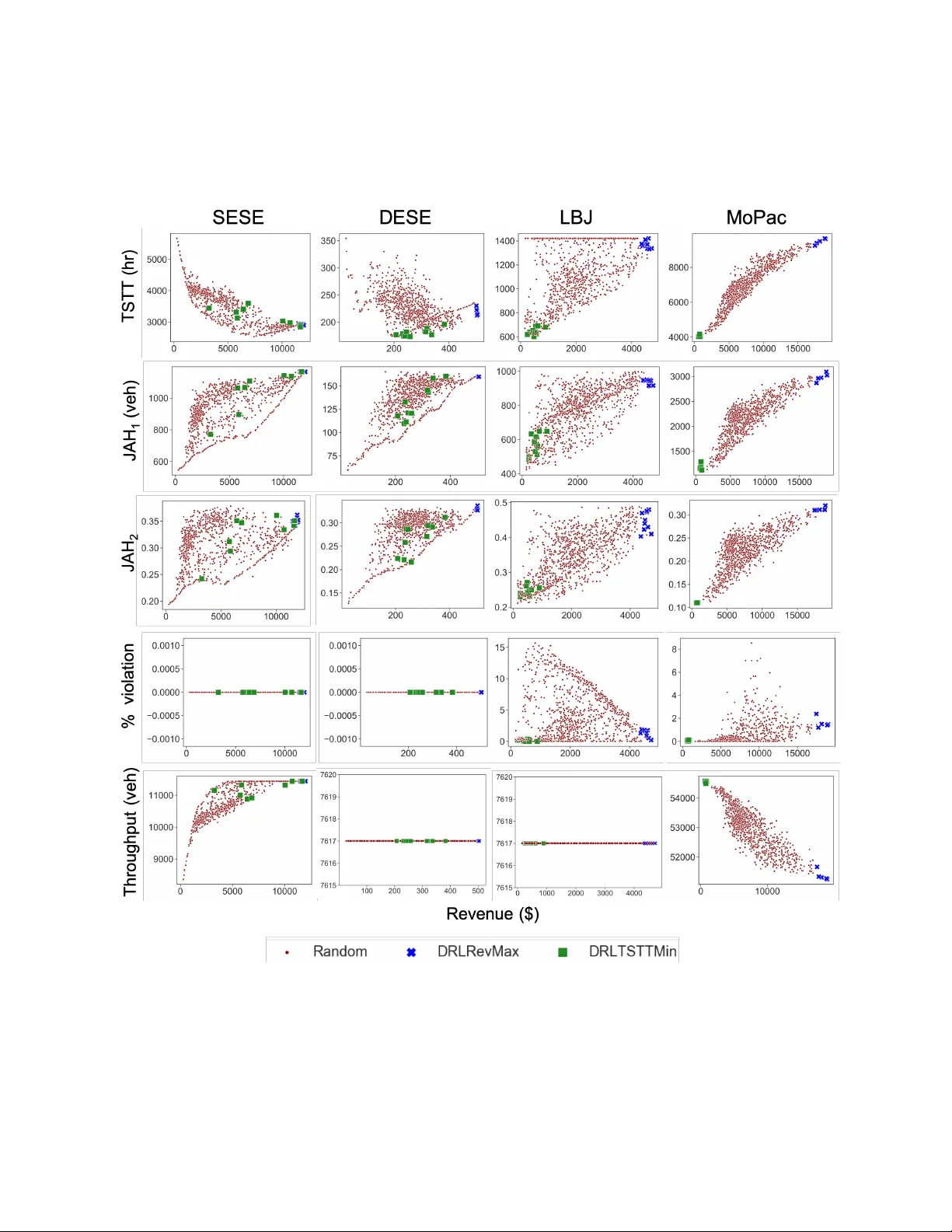
Deep Reinforcemen t Learning Algorithm for Dynamic Pricing of Express Lanes with Multiple Access Lo cations V enktesh P andey , Ev ana W ang, and Stephen D. Bo yles ∗ Abstract This article dev elops a deep reinforcement learning (Deep-RL) framew ork for dynamic pric- ing on managed lanes with multiple access lo cations and heterogeneity in tra v elers’ v alue of time, origin, and destination. This framework relaxes assumptions in the literature by con- sidering m ultiple origins and destinations, m ultiple access locations to the managed lane, en r oute diversion of tra velers, partial observ ability of the sensor readings, and sto c hastic demand and observ ations. The problem is formulated as a partially observ able Mark ov decision process (POMDP) and p olicy gradien t metho ds are used to determine tolls as a function of real-time ob- serv ations. T olls are mo deled as contin uous and sto c hastic v ariables, and are determined using a feedforward neural net work. The method is compared against a feedback con trol metho d used for dynamic pricing. W e sho w that Deep-RL is eﬀective in learning toll p olicies for maximizing rev enue, minimizing total system trav el time, and other joint weigh ted ob jectiv es, when tested on real-w orld transportation net works. The Deep-RL toll p olicies outperform the feedback con- trol heuristic for the reven ue maximization ob jective b y generating reven ues up to 9.5% higher than the heuristic and for the ob jectiv e minimizing total system trav el time (TSTT) by gener- ating TSTT up to 10.4% low er than the heuristic. W e also propose reward shaping metho ds for the POMDP to ov ercome undesired behavior of toll p olicies, like the jam-and-harvest behavior of reven ue-maximizing policies. Additionally , we test transferabilit y of the algorithm trained on one set of inputs for new input distributions and oﬀer recommendations on real-time imple- men tations of Deep-RL algorithms. The source co de for our exp eriments is av ailable online at https://github.com/venktesh22/ExpressLanes_Deep- RL . Keyw ords: Managed lanes, Express lanes, High occupancy/toll (HOT) lanes, Dynamic pricing, Deep reinforcement learning, T raﬃc control, F eedback con trol heuristic. ∗ All authors are aﬃliated with the Department of Civil, Architectural and En vironmental Engineering, The Univ ersity of T exas at Austin, Austin, TX, 78712 USA. Corresponding author’s e-mail: venktesh@utexas.edu . 1 1 In tro duction 1.1 Bac kground and Motiv ation Priced managed lanes (MLs), also referred to as express lanes or high-o ccupancy/toll lanes, are increasingly b eing used b y many cities to mitigate traﬃc congestion and provide reliable tra vel time by using the existing capacit y of the roadwa y . As of January 2019, there are 41 managed lane pro jects across the United States [6]. On these lanes, trav elers pay a toll whic h changes with the time of da y , or dynamically based on the congestion pattern, to experience less congested trav el time from their origin to their destination. In recent years, managed lane net works hav e b ecome increasingly complex, spanning longer corridors and ha ving m ultiple en trance and exit lo cations. F or example, the LBJ TEXpress lanes in Dallas, TX ha v e 17 en trance ramps and 18 exit ramps, and three tolling segmen ts with diﬀeren t time-v arying toll v alues [14]. Dynamic pricing for express lanes with multiple ac cess p oin ts is a complex control problem due to the heterogeneity in lane choice b eha vior of trav elers belonging to diﬀeren t classes. V ehicles diﬀer in their v alues of time and their destination of tra vel, b oth of which impact the pricing structure. Predicting driver b eha vior is diﬃcult. A recent study show ed that a binary logit mo del, commonly used for mo deling lane choice, is inadequate in predicting heterogeneit y in lane c hoice decisions [4]. Sev eral dynamic pricing algorithms ha ve b een explored in the literature that optimize tolls under v arying assumptions on driver b eha vior. These include metho ds using sto chastic dynamic program- ming [32], hybrid mo del predictive control (MPC) [27, 28], reinforcemen t learning (RL) [20, 36], and appro ximate dynamic programming [19]. While these algorithms do well against existing heuristics, they make some or all of the following restricting assumptions, whic h we relax: 1. Restricted access for tra velers: tra velers do not exit the managed lane once they enter till their exit is reac hed [32, 36] and that they only consider the ﬁrst entry p oint as the dec ision p oin t for the lane choice decision [27] 2. F ully observ able system: toll op erators hav e access to measuremen ts of traﬃc density through- out the net w ork for optimizing tolls [19, 20, 27, 32, 36] 3. Ignored trav eler heterogeneit y: a single v ehicle class is considered with a single origin and destination [19, 32, 36] 4. Simpliﬁed traﬃc dynamics: for example, the ﬂow dynamics on general-purpose lanes are assumed indep enden t of vehicles using the managed lane [32]; or the prop ortion of ﬂo w split at diverge p oin ts is assumed iden tical for all origins [27] In addition, there are relatively few analyses on the conﬂict b etw een optimization of multiple ob jectives with realistic constrain ts. Pandey and Boyles [19] sho wed that the rev en ue-maximizing tolls exhibit a jam-and-harvest (JAH) nature where the parallel general purpose lanes (GPLs) are 2 in tentionally jammed to congestion earlier in the sim ulation to harvest more rev enue to w ards the end. Handling such undesirable b eha vior of optimal p olicies has not b een studied in the literature. F urthermore, practical applicabilit y of these algorithms in the real world en vironmen ts is a less- explored question. Algorithms that optimize prices using a simulation model can be applied in real- time using lookup tables. Ho wev er, the transferabilit y analysis of suc h lo okup tables to new input distributions is not considered [19, 32, 36]. The hybrid MPC algorithm in T an and Gao [27] uses a sim ulation mo del to predict boundary traﬃc as an exogenous input and an optimization model that incorp orates real-time measuremen ts of traﬃc densities and vehicle queue length to optimize tolls o ver a ﬁnite horizon. The computation time for solving the mo del is in the range of 1 . 2–2 . 6 seconds for a 30 seconds optimization horizon, suﬃcient for a real-time implementation; how ev er, the tests conducted are limited with analysis only on one test netw ork under t wo scenarios of demand, assuming full observ ability of the system. Solving an MPC-based mo del with heterogeneous v ehicle classes and partial observ ability of the system is complex and not fully studied. W e th us require scalable algorithms for real-w orld net works that relax the assumptions on driver behavior and traﬃc ﬂo w, and transfer well from simulation settings to new input distributions. In this article, w e use deep reinforcement learning (Deep-RL) algorithms for optimizing tolls while relaxing simplifying assumptions in the earlier literature. In the recent y ears, Deep-RL algorithms ha ve b een successfully used for applications in pla ying computer games lik e Atari and planning motion of h umanoid rob ots lik e MuJoCo [2]. Similar algorithms ha ve b een applied in the areas of traﬃc signal control [25], activ e traﬃc managemen t (like ramp metering) [3], and control of au- tonomous vehicles in mixed autonom y [31]. These traﬃc con trol applications indicate the usefulness of Deep-RL algorithms for solving the dynamic pricing problem for managed lanes with complex access structure. W e form ulate and solve the dynamic pricing problem as a Deep-RL problem, and compare its p erformance against an existing feedback con trol metho d. W e focus our attention on pricing al- gorithms that rely on real-time densit y observ ations using sensors (suc h as lo op detectors) lo cated only at certain lo cations around the net work without access to an y information ab out the demand distribution or driv er characteristics lik e the v alue of time (VOT) distribution. Our framew ork th us relaxes assumptions in the literature by considering multiple origins and destinations, m ulti- ple access points to the managed lane facilit y , en r oute diversion of vehicles at each div erge point, and partial observ ability of the systems. W e in v estigate the usefulness of Deep-RL as a to ol for dynamic pricing, and explain its adv an tages and limitations b y exp eriments on four diﬀerent test net works. 1.2 Related W ork Man y control problems hav e b een studied in the area of transp ortation engineering. These include activ e traﬃc managemen t strategies suc h as ramp metering, v ariable sp eed limits, dynamic lane use 3 con trol, and adaptive traﬃc signal control (A TSC). Control problems in the area of transp ortation are broadly solv ed using three methods: op en-loop optimal control m ethods (that solv e the optimal con trol problem without incorporating real-time measuremen ts), closed-loop control metho ds lik e MPC (that incorp orate the feedback of real-time measurements and optimize o ver a rolling horizon), and lately RL metho ds where the optimal con trol is learn t with an iterativ e in teraction with the en vironment, p ossibly in sim ulated oﬄine settings which can then b e translated in real-time settings. A broad o verview of all control problems in the transportation domain is out of scop e of this article. The managed lane pricing problem is also a traﬃc control problem, where the chosen con trol directly impacts the driver b eha vior and th us the congestion pattern. There are three component mo dels to the ML pricing problem [10]: a lane choic e mo del that determines how tra velers c ho ose a lane given the tolls and tra vel times, a tr aﬃc ﬂow mo del that mo dels the in teraction of vehicles in sim ulated environmen ts, and a tol l pricing mo del which determines the toll pricing ob jectiv es and how the optimization problem is solved to ac hieve the b est v alue of the ob jectiv e. Pandey [18] presen ted a tabular comparison of comp onen t mo dels for the existing mo dels in the literature. In this research, w e focus on the tol l pricing mo dels . T oll pricing mo dels for MLs with a single access p oin t are commonly studied. Gardner et al. [10] argued that for ML with a single en trance and exit, the tolls minimizing the total system trav el time (TSTT) also utilize the managed lanes to full capacity at all times. The authors developed an analytical form ulation for tolls minimizing TSTT which send as man y vehicles to the ML at each time step as is the capacity of the lane. Lou et al. [16] used a self-learning approac h for optimizing toll prices where the a verage V OT v alues were learnt using real-time measurements. T oledo et al. [28] used a rolling horizon approach to optimize future tolls with predicted demand from traﬃc sim ulation; how ever, the metho d of exhaustiv e search to solve the non-con vex con trol problem do es not scale w ell for large managed lane net w orks. F or managed lanes with multiple access p oin ts, T an and Gao [27] presented a form ulation where the prop ortion of vehicles en tering the managed lane is optimized instead of directly optimizing the toll prices. The authors show ed a one-to-one mapping betw een optimal toll prices and the prop ortion v alues, and transformed the control problem in to a mixed-integer linear program which can b e solved eﬃcien tly for net works with multiple access p oin ts. Dorogush and Kurzhanskiy [8] used a similar metho d and optimized split ratios at eac h diverge, which are then used to determine toll prices; ho wev er, their analysis ignored the v ariation of incoming ﬂo w at each diverge. Apart from these optimal control based metho ds, Zh u and Ukkusuri [36] and P andey and Boyles [19] used RL methods, where the con trol problem is form ulated as a Marko v decision process (MDP) and the v alue function (or its equiv alent Q-function) is learned by iterative in teractions with the en vironment. Ho wev er, the tests are conducted for discrete state and action spaces assuming full observ ability of the system. The present article is guided b y adv ances in RL metho ds, and impro ves these earlier RL-based approac hes for dynamic pricing. Deep-RL improv es traditional RL b y using deep neural net works as function appro ximators, whic h 4 has been eﬀectiv e in v arious con trol problems. See Arulkumaran et al. [2] for a survey of Deep- RL applications. Deep-RL works w ell because it learns the system/en vironment characteristics b y rep eated interactions with the en vironment, without requiring kno wledge of the comp onen t mo del. It is a form of end-to-end learning where learning can b e done using direct observ ations, in contrast to the sequen tial learning metho ds which use observ ations to calibrate comp onent mo dels like the input V OT distribution and then optimize toll prices. Classical con trol metho ds that rely hea vily on the mo del behind the system can b e v ery complex, esp ecially for the dynamic pricing problem [27]. These metho ds require simplifying traﬃc ﬂow and driv er b ehavior assumptions for relaxing the non-conv ex optimal con trol problem. Considering the amount of uncertaint y in a dynamic pricing system, Deep-RL based metho ds can prov e eﬀective and we in vestigate this as a h yp othesis in this article. Application of Deep-RL algorithms for traﬃc con trol problems is not new. Belletti et al. [3] devel- op ed an “expert-level” control of coordinated ramp metering using Deep-RL methods with m ultiple agen ts and achiev ed precise adaptive metering without requiring model calibration that do es better than the traditional benchmark algorithm named ALINEA. W u et al. [31] used Deep-RL algorithms to solv e the control problem of selecting the acceleration and brak e of multiple autonomous v ehi- cles (A Vs) under conditions of mixed human v ehicles and A Vs to mitigate traﬃc congestion. When compared against classical approaches, their approach generated 10-20% low er TSTT. Other appli- cations of Deep-RL algorithms are in the domain of A TSC including traditional one signal con trol [11, 25], coordinated control of traﬃc signals [29], and large-scale m ultiagent control using Deep-RL metho ds [5]. See Y an et al. [33] for a review of RL algorithms in the area of A TSC. Inspired b y the open-source b enc hmark called FLO W [31], whic h is a microscopic deep reinforce- men t learning framework for traﬃc management, the multiclass mesoscopic traﬃc ﬂow environmen t dev elop ed in this article is made open-source so future tests on improving the algorithms for dy- namic pricing can b e b enc hmark ed. 1.3 Con tributions and Outline The key con tributions of this article are: • W e demonstrate the usefulness of Deep-RL algorithms for solving dynamic pricing con trol problem under partial observ abilit y , and sho w that it p erforms w ell against existing heuristics, without requiring restricting assumptions on driv er b eha vior or traﬃc dynamics. • W e apply multi-ob jectiv e optimization methods for join t optimization of m ultiple ob jectives and ov ercome undesirable JAH c haracteristics of rev enue-maximizing optimal p olicies. • W e conduct tests to verify the transferabilit y of learned Deep-RL algorithms to new input distributions and mak e recommendations on real-time implementation of the algorithm. • W e develop an op en-source framew ork for dynamic pricing using multiclass cell transmission mo del a v ailable for benchmarking future dynamic pricing exp erimen ts. 5 The rest of the pap er is organized as follows. Section 2 in tro duces the notation and presen ts the details of the mo del. Section 3 explains the chosen Deep-RL algorithms and the feedbac k control heuristic against whic h the algorithm is compared. Section 4 presents the experimental analysis of Deep-RL algorithms on four test netw orks and discusses transferability analysis, multi-ob jectiv e optimization, and comparison of the p erformance with another heuristic. Section 5 concludes the pap er and suggests topics for future w ork. 2 Mo del for Deep Reinforcemen t Learning 2.1 Net w ork Notation Consider the directed net work shown in Figure 1 whic h is an abstraction of a managed lane netw ork. The upp er set of links form MLs, the lo wer set of links form GPLs, and the ramps connect the t wo lanes at v arious access points. As we describ e the netw ork, we lab el the assumptions made in our mo del as “A#”. W e also lab el ideas for future work as “FW#”. O a d c b g k f l D i h Managed lane General purpos e lane O D e j Figure 1: Managed lane netw ork with multiple en trances and exits where links with higher thic kness are tolled, and links with a b o x are observ ed by the toll operator Let N represen t the set of all no des and A = { ( i, j ) | i, j ∈ N } represent the set of all links in the net work. Let N o denote the set of all origins and N d denote the set of all destinations. W e assume that origins and destinations connect to the net work through no des on the GPLs (A#1) and the only w ay to access the MLs is through on-ramps leading to wards the lane. This is a reasonable assumption as most current ML installations allow access to MLs only through ramps from the GPL. If there is a direct access to the ML from outside the net work, the current framework can still b e used b y appropriately adjusting the lane c hoice mo del explained in Section 2.2. The time horizon is divided in to equal time steps, eac h ∆ t units long. The set of all time perio ds is given by T = { t 0 , t 1 , t 2 , . . . , t T / ∆ t } , where T , an in tegral m ultiple of ∆ t , is the time horizon. T olls are up dated after every ∆ τ = m ∆ t time units, where m is a p ositiv e integer ﬁxed by the tolling agency . Deﬁne T τ = { k | t km ∈ T , where k ∈ { 0 , 1 , 2 , . . . }} as the set of time p erio ds where tolls are updated, indexed in increasing order of p ositiv e in tegers. Then, | T τ | = T / ∆ τ + 1. F or 6 example, Figure 2 sho ws diﬀerent elements of time where m = 4 and T = 16∆ t . F or the ﬁgure, T = { t 0 , t 1 , t 2 , . . . , t 16 } and T τ = { 0 , 1 , 2 , 3 , 4 } . Δ𝑡 Δ𝜏 𝑡 $ 𝑡 𝑡 % 𝑡 & 𝑡 ' 𝑡 ( 𝑡 ) 𝑡 * 𝑡 + 𝑡 , 𝑡 - 𝑡 %$ 𝑡 %% 𝑡 %& 𝑡 %' 𝑡 %( 𝑡 %) 𝑡 %* 0 1 2 3 4 Toll update steps Simulation update steps Figure 2: Represen tation of a time scale The demand betw een an origin and a destination is a random v ariable. A toll operator does not kno w the demand distribution, but only relies on the observ ed realizations of demand. How ever, for simulation purp oses, we mo del the demand of vehicles from origin r ∈ N o to destination s ∈ N d at time t ∈ T to b e a rectiﬁed Gaussian random v ariable with mean d rs ( t ) and standard deviation σ d , and ignore correlations of demand betw een diﬀerent origin-destination (OD) pairs and across time. The mean demand d rs ( t ) can b e estimated by observing the historical data of the managed lane facility or from the regional mo del. Let V denote the set of all v alues of VOT (assumed to b e a discrete distribution for the p opulation, A#2) and p v b e the prop ortion of demand with VOT v , for any v ∈ V . The p v v alues are unknown to a toll op erator. F or simulation purp oses, we choose the VOT distribution ( p v | v ∈ V ) and σ d to b e identical for all origin-destination pairs. Though dynamic traﬃc assignmen t mo dels ha v e b een used in the literature for optimization of toll prices for express lanes [35], we focus on real-time optimization of toll prices and ignore route-c hoice equilibration of tra velers (A#3). W e th us assume tra velers base their decisions only on real-time information provided at div erge p oin ts. The lane c hoice models are discussed in Section 2.2. T raﬃc ﬂo w models can either b e microscopic or macroscopic. With the exception of Belletti et al. [3], all other Deep-RL models in transp ortation domain use microsimulation to capture the v ehicle-to-vehicle in teractions. In this article, we use macroscopic mo dels to represen t traﬃc ﬂow for the simplicity they provide. In contrast to the cell-based representation of managed lane net work in macroscopic traﬃc mo dels from the literature, where MLs and GPLs are mo deled as part of the same cell [8, 27, 32], we divide each link into individual cells, where the links for GPLs are separate from that of MLs. This c hoice lets us use the cell transmission mo del (CTM) equations from Daganzo [7] for mo deling traﬃc ﬂo w. Let C ( i,j ) represen t the set of all cells for link ( i, j ) ∈ A and C = S ( i,j ) ∈ A C ( i,j ) denote the set of all cells in the net work. The length of eac h cell c ∈ C , denoted b y l c , is determined as usual (the distance tra veled at free ﬂo w in time ∆ t ) [7], and is assumed constant for all links in the netw ork (A#4). W e thus require all link lengths to b e integral m ultiples of the cell length. Let l ij , ν ij , q max ,ij , w ij , and k jam ,ij represen t the length, free-ﬂo w sp eed, 7 capacit y , back-w a ve sp eed, and jam density , respectively , for link ( i, j ) ∈ A as its fundamental diagram parameters, whic h we assume has a trap ezoidal shap e (A#5). A toll operator is assumed to manage the toll rate at eac h on-ramp and div erge p oin t b ey ond a div erge on a ML (A#6). W e assume this toll structure in con trast to the generic structure of separate toll v alues for eac h origin-destination (OD) pair, like in Y ang et al. [32] and T an and Gao [27], b ecause it inherently mo dels the constrain t that tra veling longer distance on the ML levies a higher toll than trav eling shorter distance. F or a detailed discussion on v arious options to c harge toll on a managed lane net work with m ultiple accesses, see Pandey and Boyles [21]. Let A toll represen t the links where tolls are collected. Figure 1 highlights these links in b old. W e denote the toll charged on link ( i, j ) ∈ A toll for any t ∈ T b y β ij ( t ). 2.2 Lane Choice Mo del T rav elers make routing decisions at eac h div erge locations while tra veling tow ards their destination. No des a, c, f , and h are the diverge lo cations for the netw ork in Figure 1. At eac h div erge no de, tra velers receiv e information ab out the current tra vel time and toll v alues. W e assume that the information ab out the curren t trav el time is provided by measuring instantaneous trav el time (A#7), and that all trav elers mak e their lane choice decision only using the instantaneous/real- time information and do not rely on historic information (obtained from prior exp erience) for making lane choices (A#8). Assumptions A#7 and A#8 are only made for simulation purposes, as the Deep-RL mo del only requires the realization of lane c hoice by each tra veler in form of observed densit y measurements at detector lo cations. If we hav e an estimate of experienced trav el time on eac h route, the sim ulations can b e based on exp erienced tra v el time. Assumptions A#3 and A#8 are related: b ecause w e assume no prior exp erience for the drivers, users do not ﬁnd an equilibrium o ver route c hoices. Considering dynamic equilibrium while optimizing a dynamic sto chastic con trol is a complex problem and will b e studied as part of the future w ork (FW#1). There are sev eral mo dels prop osed in the literature to model lane choice of tra velers, including a binary logit model that mo dels sto c hastic lane c hoice of tra velers o ver t wo routes connecting curren t div erge to the destination, and a decision route mo del that ev aluates deterministic lane c hoice of multiple vehicle classes comparing utilities o ver a set of routes connecting curren t div erge to the merge after the ﬁrst exit from the ML. F or a detailed discussion on the decision route mo del, refer to P andey and Bo yles [19]. A recen t analysis in Pandey and Bo yles [21] sho wed that a decision route model has the least error compared to the optimal route choice mo del for rational trav elers; ho wev er, a logit mo del can capture irrational driver b eha vior, where a rational tra veler is deﬁned as the one who alwa ys chooses the route minimizing her utility . Conceptually , the lane c hoice mo dels can b e categorized based on three characteristics: the n umber of routes o ver which tra velers compare the utility , whether or not the lane choice is sto c hastic/deterministic, and the heterogeneit y in vehicles’ v alue of time (single class vs multiple classes). T able 1 shows the com binations of categories and mo dels used in the literature. Certain combination ha ve not 8 b een used directly , but they could b e used. F or example, com bining decision routes with sto c hastic lane c hoice can result in mo dels like multinomial logit or mixed logit, but the assumption that the c hoices are indep enden t may not hold true (the choices in this setting b eing the diﬀerent routes). T able 1: Categorization of lane choice mo dels for managed lanes with m ultiple entrances and exits Num b er of V OT classes Num b er of routes o v er whic h the utility(s) is (are) compared Deterministic or Stochastic Reference(s) in the literature using this lane c hoice Single Tw o Deterministic [10] Single Tw o Sto c hastic [27][28][36][32] Single Decision routes Deterministic None Single Decision routes Sto c hastic None Multiple Tw o Deterministic [9] Multiple Tw o Sto c hastic None Multiple Decision routes Deterministic [19],[20] Multiple Decision routes Sto c hastic None The Deep-RL algorithm developed in this article is agnostic to the lane c hoice model. F or sim u- lation purp oses, we fo cus our atten tion on t wo mo dels: m ultiple V OT classes with tw o routes and sto c hastic choice ( multiclass binary lo git mo del ) and multiple V OT classes with decision routes and deterministic c hoice ( multiclass de cision r oute mo del ). F or simulation purposes, w e ev aluate the utilit y of a route as the linear combination of the toll and route’s tra vel time, con verted to the same units using the V OT for the class (A#9). 2.3 P artially Observ able Mark o v Decision Pro cess MDPs are a discrete time sto c hastic control pro cess that pro vide a framew ork for solving problems that in volv e sequen tial decision making [26]. At eac h time step, the system is in some state . The decision mak er tak es an action in that state , and the system transitions to the next state depending on the transition probabilities, whic h are only a function of the current state and the action taken (called the Mark ov property). Giv en an action , this transition from one state to the other generates a reward for each time step and the decision maker seeks to maximize the exp ected reward across all time steps. Con trol problems in transp ortation do not necessarily ha ve the Marko v prop ert y b ecause of the temp oral dep endence of congestion pattern. Ho wev er, by including the simulation time as part of the state, they can be form ulated as an MDP . P artially observ able Marko v decision pro cesses (POMDPs) are MDPs where the state at an y time step is not kno wn with certain ty , that is, the state is not fully observ able. F or the dynamic pricing problem where a toll op erator do es not ha v e access to traﬃc information throughout the net w ork but only at certain locations, POMDPs are a suitable c hoice. W e deﬁne the control problem for determining the optimal toll as an POMDP with follo wing comp onen ts: 9 • Timestep : T olls are to b e optimized ov er a ﬁnite time horizon for each time k ∈ T τ . A ﬁnite horizon can represen t a morning or an ev ening p eak p erio d on a corridor, or an en tire day . • State : W e ﬁrst deﬁne x z c ( t ) as the num b er of v ehicles in cell c ∈ C b elonging to class z ∈ Z at time t ∈ T , where Z = { ( v , d ) | v ∈ V , d ∈ N d } is the set of all classes, disaggregated by the VOT v alue and the destination of the v ehicle (the origin of a v ehicle do es not inﬂuence lane choice once the v ehicle is on the road and is thus ignored). F or ML netw orks where high o ccupancy vehicles pa y a diﬀerent toll than single/low o ccupancy vehicles, we can extend Z to include the o ccupancy level of v ehicles, but we lea ve that analysis for future work (FW#2). The dimensionality of Z impacts the computational p erformance of the multiclass cell transmission model. Similar to the non-atomic ﬂo w assumption commonly used in the transp ortation literature, we consider x z c ( t ) to b e a non-negativ e real num b er, rather than an in teger. W e denote the state of the POMDP b y s comprising of the current toll up date step k ∈ T τ and the v alues x z c ( t k ∆ τ ) for all cells c ∈ C and class z ∈ Z . Thus, the state space S can b e written as Equation (2.1). Allowing ∆ τ to be greater than ∆ t ( m > 1) reduces the size of state space compared to choosing m = 1, which impro ves the computational eﬃciency . S = { ( k , x z c ( t k ∆ τ )) | k ∈ T τ , c ∈ C , z ∈ Z } (2.1) • Observ ation : In our mo del, the observ ation is done using lo op detectors. The detectors measure the total num b er of v ehicles going from one cell to the next and thus cannot distin- guish b et ween v ehicles b elonging to diﬀerent classes, so the state is not fully observ able. This is an adv antage of the proposed mo del, contrasting with the commonly-used full observ ability assumption [27, 34]. The observ ation space dep ends on the lo cation of detectors. W e conduct sensitivit y analyses with resp ect to c hanges in the observ ation space later in the text. Let o ( s ) denote the observ ation vector for state s and comprise of the measurement of total num b er of v ehicles on each link ( i, j ) ∈ A loop ⊆ A whic h has a lo op detector installed at b eginning and end. 1 That is, o ( s ) = { P z ∈ Z P c ∈ C (i,j) x z c ( t k ∆ τ ) | ( i, j ) ∈ A loop } . W e assume that we can learn the total num b er of v ehicles on any link b y tracking the n um b er of vehicles entering the link (measured at an upstream detector) and the num b er of vehicles lea ving the link (measured at a downstream detector) (A#10). The actual observ ation is assumed to be Gaussian random v ariable with the mean as sp eciﬁed and the standard deviation σ o whic h mo dels the noise in lo op detector measurements. W e pro ject negative v alues of observ ation, if an y , to zero. • Action : Action a in state s is the toll β ij ( t k ∆ τ ) charged for a toll link ( i, j ) ∈ A toll , where β ij ( · ) ∈ [ β min , β max ]. The action is modeled as a contin uous v ariable; the v alues can b e rounded to nearest ten th of a cent or dollar if desired. • T ransition function : The transition of the POMDP from a state s to a new state s 0 giv en action a , is go verned b y the traﬃc ﬂo w equations from the CTM mo del which incorp orates 1 F or Figure 1, A loop = { ( o, a ) , ( a, c ) , ( c, e ) , ( d, f ) , ( g , h ) , ( h, j ) } . 10 the lane choice behavior of tra velers. F or simulation purposes, we assume that traﬃc ﬂo w throughout the netw ork is deterministic except at div erges where the lane choices of trav elers ma y b e sto c hastic (A#11). W e use a multiclass version of the CTM mo del similar to the mo del in Pandey and Boyles [19]. • Rew ard : The reward obtained after taking action a in state s , denoted b y r ( s, a ), dep ends on the choice of tolling ob jectiv e. W e consider tw o ob jectiv es, rev enue maximization and total system tra v el time (TSTT) minimization, with follo wing deﬁnitions of reward: – Rev enue maximization: r RevMax ( s, a ) = ( k +1)∆ τ − 1 X x = k ∆ τ X ( i,j ) ∈ A toll   β ij ( t k ∆ τ ) X ( h,i ) ∈ A y hij ( t x )   (2.2) where y hij ( t ) is the total ﬂo w moving from link ( h, i ) ∈ A to ( i, j ) ∈ A from time step t to time step t + ∆ t – T otal system tra vel time minimization: r TSTTMin ( s, a ) = −   ( k +1)∆ τ − 1 X x = k ∆ τ X c ∈ C X z ∈ Z x z c ( t x )   (2.3) where the negativ e sign is used to ensure that rew ard maximization is equiv alent to TSTT minimization. F or the dynamic pricing problem, rev enue-maximizing tolls often ha ve a JAH nature where the GPLs are jammed to congestion earlier in the sim ulation to attract more trav elers tow ards the ML later in the sim ulation generating more reven ue [12, 19]. This undesirable characteristic of optimal p olicy is also seen in other applications of RL. F or example, for A TSC a simpler deﬁnition of reward that maximizes amoun t of ﬂo w during a cycle may lead to “evil” optimal p olicies, where the controller agent holds congestion on the mainline and then gains a larger reward b y extending the greens for the main approac h [25]. Similarly , V an der P ol and Olieho ek [30] sho w that with inappropriate deﬁnitions of rew ard, the signal con trol p olicy may ha ve un usual ﬂips from green to red. T o ov ercome the undesired JAH nature, w e use rew ard shaping methods that modify the rew ard def- initions suc h that the optimal p olicies ha ve less or no JAH behavior (discussed later in Section 4.4). F or reward shaping, we quantify the JAH b eha vior using t wo statistics deﬁned as a numeric v alue at the end of sim ulation. The ﬁrst statistic, JAH 1 , measures the maxim um of diﬀerence b et ween the num b er of vehicles in GPLs to the num b er of vehicles in MLs across all time steps. It is deﬁned as in Equation (2.4), where A GPL ( A ML ) are links on the GPL (ML). 11 JAH 1 = max t ∈ T   X ( i,j ) ∈ A GPL X c ∈ C ( i,j ) X z ∈ Z x z c ( t ) − X ( i,j ) ∈ A ML X c ∈ C ( i,j ) X z ∈ Z x z c ( t )   (2.4) The v alue of JAH 1 is dep enden t on netw ork prop erties lik e num b er of lanes in GPLs and MLs. W e also deﬁne an alternate statistic JAH 2 that is net work indep enden t. W e ﬁrst deﬁne ζ ( t ), as in Equation (2.5), as the diﬀerence b et ween the ratio of curren t n umber of vehicles to the maxim um n umber of v ehicles allow ed in eac h cell (corresponding to jam density) for all cells on GPLs with that of MLs. ζ ( t ) = P ( i,j ) ∈ A GPL P c ∈ C ( i,j ) P z ∈ Z x z c ( t ) P ( i,j ) ∈ A GPL P i ∈ C ( i,j ) l ij k jam ,ij − P ( i,j ) ∈ A ML P i ∈ C ( i,j ) P z ∈ Z x z i ( t ) P ( i,j ) ∈ A ML P i ∈ C ( i,j ) l ij k jam ,ij (2.5) JAH 2 can then b e deﬁned as a maximum v alue of ζ ( t ) across all time steps, as in Equation (2.6). The v alue of JAH 2 v aries b et ween [ − 1 , 1] with a high p ositiv e v alue indicating more congestion on GPLs b efore congestion set in the ML. JAH 2 = max t ∈ T ζ ( t ) (2.6) F or the given POMDP , a p olicy π θ ( a | o ( s )) denotes the probabilit y of taking action a giv en obser- v ation o ( s ) in state s . W e consider sto c hastic p olicies parameterized b y a vector of real parameters θ . F or example, for a p olicy replaced by a neural netw ork, θ represen ts the ﬂattened weigh ts and biases for the nodes in the netw ork. Since the action space for the POMDP is con tinuous, the neural net work outputs the mean of the Gaussian distribution of tolls which is then used to sam- ple con tinuous actions. F or simplicit y in Deep-RL training, w e assume the co v ariance of the join t distribution of actions to b e a diagonal matrix with constant diagonal terms (A#12). Figure 3 sho ws a sc hematic of the parameterized represen tation of the p olicy whic h takes in the input of observ ations across the netw ork and returns the mean of the Gaussian toll v alues for all toll links. MLP stands for m ulti-lay er p erceptron which is a feedforward neural netw ork architecture. Observation vector MLP neural network Mean of the Gaussian toll at every toll entrance Figure 3: Abstract representation of the policy 12 2.4 Episo dic Reinforcemen t Learning In an episo dic reinforcement learning problem, an agent’s exp erience is broken in to episo des, where an episo de is a sequence with a ﬁnite n um b er of states, actions, and rew ards. Since the POMDP in tro duced in the previous subsection is ﬁnite-horizon, the sim ulation terminates at time T / ∆ t . Th us, an episo de is formed by a sequence of states, actions, and rewards for each time step k ∈ T τ . W e ﬁrst deﬁne a tra jectory ℵ as a sequence of states and actions visited in an episode, that is ℵ = ( s 0 , a 0 , s 1 , a 1 , · · · , s | T τ |− 1 ), where s k is same as the state deﬁned earlier indexed by the time k in that state. Let r ( s k , a k ) b e denoted b y r k for all k ∈ T τ . The goal of the RL problem is to ﬁnd a p olicy that maximizes the exp ected reward ov er the entire episo de. The optimization problem can then be written as following: max π θ ( · ) J ( π θ ) = E ℵ [ R ( ℵ ) | π ] (2.7) R ( ℵ ) = X k ∈ T τ r k , (2.8) where, E ℵ [ R ( ℵ ) | π ] = R R ( ℵ ) p π ( ℵ ) d ℵ is the exp ected rew ard o ver all p ossible tra jectories obtained after executing p olicy π with p π ( ℵ ) as the probabilit y distribution of tra jectories obtained by executing p olicy π . 2 W e do not discoun t future rewards b ecause tolls are optimized o ver a short time p erio d (lik e a da y or a morning/evening p eak). W e deﬁne a few additional terms used later in the text. Let V π ( s k ) = E ℵ P | T τ | k 0 = k r k 0 b e the v alue function which ev aluates the exp ected rew ard obtained from state s k till the end of episo de following p olicy π . Similarly , w e deﬁne the Q-function, denoted by Q π ( s k , a k ), as the exp ected rew ard obtained till the end of episo de from state s k after taking action a k and following p olicy π thereafter. Last, the adv an tage function A π ( s k , a k ) = Q π ( s k , a k ) − V π ( s k ), deﬁned as the diﬀerence betw een Q-function and v alue function, determines ho w m uch b etter or w orse is an action than other actions on av erage, given the current p olicy . The solution of this POMDP is a v ector θ ∗ that determines the p olicy which optimizes the ob jective under certain constrain ts on the p olicy space. Commonly considered p olicy constrain ts for the dynamic pricing of express lanes include the following: 1. T olls levied for a longer distance are higher than tolls levied for a shorter distance from the same entrance: with the choice of tolling structure (assumption A#6) where tolls are charged at every div erge, this constrain t is already satisﬁed. 2. The ML is alw ays op erated at a sp eed higher than the minim um speed limit (called the speed- 2 Deﬁning an expectation conditioned ov er a function ( π ) instead of a random v ariable is a slight abuse of notation, but is commonly used in the RL literature. 13 limit constraint): in our model, w e allo w violation of this constraint on the ML. W e observe that, given the sto c hasticit y in lane choice of tra velers and demand, b ottlenec ks can o ccur at merges and div erges whic h can result in an inevitable spillo ver on managed lanes during congested cases. Thus, a hard constraint k eeping the ML congestion free throughout the learning p erio d is not useful. W e instead quan tify the violation of the sp eed-limit constraint using the time-space diagram of the cells on the ML. W e deﬁne %-violation as the prop ortion of cell-timestep pairs on the time-space diagram where the sp eed limit constraint is violated, expressed as percentage. Mathematically , %-violation = P ( i,j ) ∈ A ML P c ∈ C ( i,j ) P t ∈ T I t c | T | P ( i,j ) ∈ A ML | C ( i,j ) | × 100 (2.9) where, I t c is an indicator v ariable which is 1 if the n umber of vehicles in the cell c in time step t is higher than the desired num b er of v ehicles in the cell and 0 otherwise. The desired n umber of vehicles in each cell is determined from the density corresp onding to the minimum sp eed limit on the fundamental diagram. As discussed in Section 4, allo wing the sp eed-limit constrain t to b e violated in our mo del is not restrictive as the best-found p olicies for each ob jective ha ve %-violation v alues of less than 2% for all net works teste d. 3. T oll v ariation from one time step to the next is restricted: w e do not explicitly mo del this constrain t. If the tolling horizon is “suﬃcien tly” large (say 5 minutes), a large change in tolls from one toll up date to the next can b e less of a problem. In our exp eriments, the optimal tolls are structured and do not oscillate signiﬁcantly . 4. T olls are upp er and low er bounded b y a v alue: w e model this b y clipping the toll output by the function appro ximator within the desired range [ β min , β max ]. Next, w e discuss the solution methods used to solv e the POMDP using Deep-RL metho ds and other heuristics. 3 Solution Metho ds 3.1 Deep Reinforcemen t Learning Algorithms Deep reinforcemen t learning algorithms can b e broadly categorized into v alue-based methods and p olicy-based methods. The former metho ds try to learn the v alue functions and use approaches based on dynamic programming to solv e the problem, while the latter metho ds try to learn the p olicy directly based on the observ ations. Policy gradien t metho ds work w ell with contin uous state and action spaces, making it a preferred choice for the toll optimization problem. Deriv ative-free optimization and gradient-based optimization are t w o types of p olicy-based meth- o ds. W e fo cus on the metho ds relying on deriv atives as they are considered to b e data eﬃcient [22]. 14 Pro viding an o verview of the state-of-the-art of policy gradien t methods to solve reinforcemen t learning problems is out of the scop e of this w ork. W e refer the reader to Sc hulman [22] for ad- ditional details. In this article, we choose tw o of the commonly used algorithms for solving the problem: the v anilla p olicy gradien t (VPG) algorithm and the proximal policy optimization (PPO) metho d from Sch ulman et al. [24]. The algorithms use the deriv ative of the ob jectiv e function with resp ect to the p olicy parameters to impro ve them using sto c hastic gradien t descen t. The metho ds diﬀer in calculation of the deriv atives and the update of parameter θ . W e can express the deriv ative of J ( π θ ) with respect to θ as: ∇ θ J ( π θ ) = ∇ θ E ℵ [ R ( ℵ ) | π ] (3.1a) = ∇ θ Z ℵ P ( ℵ| θ ) R ( ℵ ) d ℵ (3.1b) = Z ℵ ∇ θ P ( ℵ| θ ) R ( ℵ ) d ℵ (3.1c) = Z ℵ P ( ℵ| θ ) ∇ θ log P ( ℵ| θ ) R ( ℵ ) d ℵ  since ∇ θ log P ( ℵ| θ ) = 1 P ( ℵ| θ ) ∇ θ P ( ℵ| θ )  (3.1d) = E ℵ [ ∇ θ log P ( ℵ| θ ) R ( ℵ )] (3.1e) = E ℵ   | T τ | X k =0 ∇ θ log( π θ ( a k | s k )) R ( ℵ )   (3.1f ) where we ﬁrst conv ert the probabilit y of a tra jectory into a pro duct of the probabilities of taking certain actions in each state, and then con v ert this pro duct into a sum. As a result, the deriv ative in the RHS of Equation (3.1f) can b e easily obtained by p erforming bac k propagation on the p olicy neural netw ork. The expectation in Equation (3.1f) can be appro ximated by av eraging o ver a ﬁnite num b er of tra jectories. Let N = {ℵ i | i ∈ 1 , 2 , ... } b e the set of tra jectories obtained using p olicy π θ ( · ). Then, w e can write: ∇ θ J ( π θ ) ≈ 1 | N | X ℵ∈ N   | T τ | X k =0 ∇ θ log( π θ ( a k | s k )) R ( ℵ )   (3.2) In the abov e formulation the lik eliho od of actions tak en along the tra jectory is aﬀected b y rew ard o ver en tire tra jectory . Ho wev er, it is more intuitiv e for an action to inﬂuence the reward obtained only after the time step when it was implemented. It can b e shown that the right hand side of the expression in Equation (3.2) is equiv alent to the follo wing expression: 1 | N | X ℵ∈ N   | T τ | X k =0 ∇ θ log( π θ ( a k | s k )) ˆ R ( k )   (3.3) 15 where ˆ R ( k ) is the reward-to-go function at time k , given b y ˆ R ( k ) = P | T τ | k 0 = k r k 0 . This new expression for the gradient of the ob jective requires sampling of few er tra jectories and generates a lo w-v ariance sample estimate of the gradient. Additionally , the v ariance can be further reduced b y using the adv antage function estimates instead of reward-to-go function [23]. VPG uses the following form for appro ximating the deriv ative: ∇ θ J ( π ( θ )) ≈ 1 | N | X ℵ∈ N   | T τ | X k =0 ∇ θ log( π θ ( a k | s k )) ˆ A k   (3.4) where ˆ A k is the estimate of adv antage function, A π θ ( s k , a k ), from current time k till the end of episo de, following the p olicy from whic h the giv en tra jectory is sampled. W e use the generalized adv antage estimation (GAE) tec hnique to estimate ˆ A k whic h requires an estimate of the v alue function [23]. W e use v alue function appro ximation to estimate of V π ( s k ) using a neural net w ork as the functional approximator. Let ˆ V φ ( s k ) denote the estimate of V π ( s k ), parameterized b y a real v ector of parameters φ . The algorithm starts with an estimate of φ ( φ 0 ) and iteratively improv es it b y minimizing the squared diﬀerence with the reward-to-go v alue from the tra jectory . The up date in φ parameters are ev aluated using Equation (3.5): φ n +1 = argmin φ 1 | N || T τ | X ℵ∈ N | T τ | X k =0  V φ ( s k ) − ˆ R ( k )  2 (3.5) More details on GAE are pro vided in Sc h ulman et al. [23]. VPG up dates the v alue of θ parameter from iteration n to n + 1 using the standard gradient ascen t form ula: θ n +1 = θ n + α ∇ θ J ( π ( θ n )) (3.6) In Equation (3.6), an inappropriate c hoice of the learning rate α can lead to large p olicy up dates from one iteration to the next which can cause the ob jective v alues to ﬂuctuate. The PPO algorithm mo diﬁes the p olicy up date to tak e the biggest p ossible improv ement using the data generated from curren t p olicy while ensuring improv emen t in the ob jectiv e. It p erforms sp ecialized clipping to discourage large c hanges in the p olicy . The p olicy up date for PPO is given by: θ n +1 = argmax θ 1 | N | X ℵ∈ N   | T τ | X k =0 min  r k ( θ ) ˆ A π θ n ( s k , a k ) , clip ( r k ( θ ) , 1 − , 1 +  ) ˆ A π θ n ( s k , a k )    (3.7) where r k ( θ ) is the ratio of probabilities following a policy and the p olicy in the current iteration 16 ( θ n ) given by Equation (3.8), and the clip ( · ) function, given by Equation (3.9), restricts the v alue of ﬁrst argumen t b et ween the next t w o argumen ts. r k ( θ ) = π θ ( a k | s k ) π θ n ( a k | s k ) (3.8) clip ( r , 1 − , 1 +  ) =          1 − , if r ≤ 1 −  r , if 1 −  < r < 1 +  1 + , if r ≥ 1 + . (3.9) The clipping op eration selects the p olicy parameters in the next iteration such that the ratio of action probabilities in iteration n + 1 to iteration n are b et ween [1 − , 1 +  ], where  is a small parameter, typically 0.01. P olicy updates for PPO can be solv ed using the Adam gradient ascen t algorithm, a v arian t of sto c hastic gradient ascen t with adaptiv e learning rates for diﬀerent parameters [13, 24]. The structure for b oth algorithms is presen ted in Algorithm 1. F or the experiments, w e dev elop a new RL environmen t for macroscopic simulation of traﬃc similar to the current RL b enc hmarks (called “gym” environmen ts) and customize the op en-source implemen tation of both algorithms pro vided b y Op enAI Spinningup [17] to work with our new en vironment. Algorithm 1 Policy gradient algorithm for dynamic pricing [17] Input: initialize policy parameters θ 0 and v alue function parameters φ 0 for do n = 0 , 1 , 2 , · · · Collect set of tra jectories N n = {ℵ n } by running p olicy π n = π θ n in the en vironmen t Compute rewards to go ˆ R k Compute adv an tage estimates using rewards-to-go and generalized adv antage estimation Up date p olicy parameters: • VPG : Estimate policy gradien ts using Equation (3.4) and up date p olicy p arameters using Equation (3.6) • PPO : Update p olicy parameters by solving Equation (3.7) using Adam gradien t ascen t algorithm Up date v alue function appro ximation parameter (used for adv antage estimation) in Equa- tion (3.5) using Adam gradient descen t end for 17 3.2 F eedbac k Con trol Heuristic W e compare the p erformance of Deep-RL algorithms against a feedbac k control heuristic based on the measurement of total n umber of v ehicles in the links on ML. W e customize the Density heuristic in P andey and Bo yles [19] to c harge v arying tolls for diﬀeren t toll links. Deﬁne ML( i, j ) as the set of links on the ML used by a trav eler up on ﬁrst en tering the ML using the toll link ( i, j ) ∈ A toll un til the next merge or diverge. F or the net work in Figure 1, ML( a, b ) = { ( b, d ) } , ML( c, d ) = { ( d, f ) } , ML( f , i ) = { ( f , i ) } , and ML( h, i ) = { ( i, k ) } . This deﬁnition allows the sets ML( i, j ) to b e mutually exclusive and exhaustiv e in the space of all links on the ML. That is, ML( i, j ) ∩ ML( k , l ) = Φ ∀ ( i, j ) ∈ A toll , ( k , l ) ∈ A toll , ( i, j ) 6 = ( k , l ) [ ( i,j ) ∈ A toll ML( i, j ) = A ML W e assume that the feedback con trol heuristic up dates the tolls for eac h toll link ( i, j ) ∈ A toll based on the density observ ations on links in ML( i, j ), that is, detectors are installed on each link in the ML and only those detectors are used to up date the toll (A#13). The toll v alue for an up date time ( k + 1) ∈ T τ is based on the toll v alue in the previous update step adjusted by the diﬀerence b et w een the desired and curren t num b ers of vehicles. The toll up date is giv en by Equation (3.10). β ij ( t ( k +1)∆ τ ) = β ij ( t k ∆ τ ) + P ×  X ML( i,j ) ( k ) − X desired ML( i,j )  (3.10) where X ML( i,j ) ( k ) is the total num b er of v ehicles on links in ML( i, j ) b efore up dating tolls at time k + 1 and X desired ML( i,j ) b e the desired v alue of the num b er of vehicles on the links in ML( i, j ). P is the regulator parameter, with units $ / v eh, con trolling the inﬂuence of diﬀerence b et ween the desired and current n um b er of vehicles on the toll up date. A t ypical desired v alue is the num b er of vehicles corresp onding to the critical density on the ML link. W e generalize the desired num b er of vehicles b y deﬁning X desired ML( i,j ) as: X desired ML( i,j ) = X ( g ,h ) ∈ ML( i,j ) η k critical , ( g ,h ) l g h (3.11) where, k critical , ( g ,h ) is the critical densit y for link ( g , h ) ∈ A and η is the scaling parameter v arying b et w een (0 , 1] that sets the desired num b er of v ehicles to a prop ortion v alue of the n um b er of vehicles at critical density . W e calibrate the feedback con trol heuristic for diﬀerent v alues of desired density and regulator parameter. In principle, both η and P can v ary with time and the toll lo cation; ho wev er, determining the “optimal” v ariabilit y in these parameters is a con trol problem in itself, exploring which is left as part of the future work (FW#3). 18 W e do not include other algorithms for comparison b ecause of lack of compatibility due to the full- observ ability assumption. The algorithms in Zhu and Ukkusuri [36] and Pandey and Boyles [19] do not scale for con tin uous action space and tolls. Comparing the p erformance of Deep-RL metho ds against the h ybrid MPC metho d in T an and Gao [27] requires extensiv e analysis and will b e a part of the future w ork (FW#4). 4 Exp erimen tal Analysis 4.1 Preliminaries W e conduct our analysis on four diﬀerent netw orks. The ﬁrst is a netw ork with single entrance and single exit (SESE) commonly used in the managed lane pricing literature. The next t wo are the double entr ance single exit (DESE) netw ork and the net work for toll segment 2 of the LBJ TEXpress lanes in Dallas, TX (LBJ). The DESE netw ork includes t wo toll lo cations for mo deling en r oute lane changes. The LBJ net work has four toll lo cations. Last is the netw ork of the northbound Lo op 1 (MoPac) Express lanes in Austin, TX. The MoPac netw ork has three entry lo cations to the express lanes and t wo exit lo cations. 2 3 5 6 4 7 8 1 1 2 4 5 6 7 3 D 1 2 5 4 3 7 10 6 11 12 9 8 (a) (b) (c) Exp res s lane s Gen eral p urp os e lane s To ll locat ions ML E xit lo cations GPL Entra nce/Exit location s Figure 4: Abstract representation of (a) single en trance single exit (SESE) net work, (b) double en trance single exit (DESE) net w ork, (c) LBJ net w ork, and (d) North b ound MoPac express lane net work (latitude-longitude lo cations of express lanes are shifted to the left to show the locations of toll p oin ts and exits from the managed lane). The tolls are collected on the links with higher thic kness. Figure 4 shows the netw orks, where the thic k lines denote the links where tolls are collected. The demand distribution for the ﬁrst three net works is artiﬁcially generated and follows a tw o-p eak pattern (refer to the original demand curv e in Figure 5a), while the demand for the MoPac net w ork is derived from a dynamic traﬃc assignment mo del of the T ra vis Count y region. There are a total 19 of 105 origin-destination pairs in the MoPac netw ork with a total demand of 49 , 273 vehicles using the netw ork in three hours of the ev ening peak. 0 1000 2000 3000 4000 5000 6000 7000 8000 0 600 1200 1800 2400 3000 3600 4200 4800 5400 6000 6600 Demand (v eh /h r ) Time (s eco nd s ) Ori g in al Dema n d Va riant 1 Va riant 2 Bot tle n ec k c apacit y (a) 0 0. 05 0. 1 0. 15 0. 2 0. 25 0. 3 0. 35 0. 4 0. 45 10 15 20 25 30 Pr opo r tion of tr a vel e r s wi th thi s V O T VO T ( $/h r ) Or ig in al VOT d is t r i bu ti o n Va r i a n t 3 (b) Figure 5: (a) Demand distributions used for the SESE, DESE and LBJ net works and its v arian ts, and (b) V OT distribution and its v arian t T able 2 shows the v alues of parameters used for diﬀerent netw orks. Five VOT classes were selected for each netw ork and the same VOT distribution was used. Figure 5b shows this VOT distribution (lab elled “original”; in some exp erimen ts we v ary this distribution.) T able 2: V alues of parameters used in the sim ulation SESE DESE LBJ MoP ac P arameter V alue Corridor length (miles) 7.3 1.59 2.91 11.1 β min $0.1 Sim ulation duration (hour) 2 2 2 3 β max $4.0 ∆ τ (seconds) 60 300 300 300 q ij (vphpl) 2200 ν ij (mph) 55 55 55 65 k jam ,ij (v eh/mile) 265 σ o (v eh/hr) 50 50 50 50 ν ij /w ij 3 σ d (v eh/hr) 10 0 0 100 ∆ t (seconds) 6 A feedforward m ultilay er perceptron w as selected as the neural net w ork. Hyp erparameter tuning w as conducted, and the arc hitecture with t wo hidden lay ers and 64 nodes in eac h la yer was selected. F or the MoPac net work, three hidden lay ers with 128 no des each w ere selected. The v alues of other h yp erparameters for Deep-RL training are as follo ws: learning rate for policy up date equals 10 − 4 , learning rate for v alue function up dates is 10 − 3 , num b er of iterations for v alue function up dates is 80, and the γ GAE and λ GAE v alues for the GAE metho d are 0 . 99 and 0 . 97, resp ectively . Each net work w as sim ulated for a n um b er of iterations ranging b et ween 100 and 200 where the av erage in each iteration was rep orted o v er 10 episo des. 20 4.2 V alidating JAH Statistics In this subsec tion, w e discuss ho w the JAH statistics deﬁned in Equations 2.4 and 2.6 are mean- ingful in capturing the jam-and-harv est nature of the rev enue maximizing proﬁles. W e sim ulate random toll proﬁles on the LBJ netw ork and record the congestion proﬁles for three v alues of JAH 2 : 0 . 22 , 0 . 33 , and 0 . 49. 3 Figures 6, 7, and 8 show the plots for the time space diagram on managed lane and general purp ose lane, and the v ariation of ζ ( t ) for three diﬀerent toll proﬁles leading to JAH 2 v alues of 0 . 22 , 0 . 33 , and 0 . 49, respectively . The scale on the time-space diagrams v aries from 0, represen ting no v ehicles, to 1, representing jam densit y . The cell id v alue on the y-axis is a six-digit num b er where the ﬁrst t wo digits are the tail no de of the link, the second tw o digits are the head no de of the link, and the last t wo digits are the index of the cell num b er on the link starting from index 1 for the ﬁrst cell near the tail node. Thus, the increasing v alue of cell IDs on the y-axis indicates the do wnstream direction. 0 258 516 774 1032 1290 1548 1806 2064 2322 2580 2838 3096 3354 3612 3870 4128 4386 4644 4902 5160 5418 5676 5934 6192 6450 6708 6966 Time (sec) 91006 91005 91004 91003 91002 91001 60906 60905 60904 60903 60902 60901 50603 50602 50601 30509 30508 30507 30506 30505 30504 30503 30502 30501 Cell ID ML Time Space Diagram 0.0 0.2 0.4 0.6 0.8 1.0 (a) 0 258 516 774 1032 1290 1548 1806 2064 2322 2580 2838 3096 3354 3612 3870 4128 4386 4644 4902 5160 5418 5676 5934 6192 6450 6708 6966 Time (sec) 81109 81107 81105 81103 81101 70802 40706 40704 40702 20409 20407 20405 20403 20401 Cell ID GPL Time Space Diagram 0.0 0.2 0.4 0.6 0.8 1.0 (b) 0 200 400 600 800 1000 1200 Time step (t) 0.0 0.1 0.2 0.3 0.4 0.5 ( t ) (c) Figure 6: Plots for JAH 2 = 0 . 22 0 258 516 774 1032 1290 1548 1806 2064 2322 2580 2838 3096 3354 3612 3870 4128 4386 4644 4902 5160 5418 5676 5934 6192 6450 6708 6966 Time (sec) 91006 91005 91004 91003 91002 91001 60906 60905 60904 60903 60902 60901 50603 50602 50601 30509 30508 30507 30506 30505 30504 30503 30502 30501 Cell ID ML Time Space Diagram 0.0 0.2 0.4 0.6 0.8 1.0 (a) 0 258 516 774 1032 1290 1548 1806 2064 2322 2580 2838 3096 3354 3612 3870 4128 4386 4644 4902 5160 5418 5676 5934 6192 6450 6708 6966 Time (sec) 81109 81107 81105 81103 81101 70802 40706 40704 40702 20409 20407 20405 20403 20401 Cell ID GPL Time Space Diagram 0.0 0.2 0.4 0.6 0.8 1.0 (b) 0 200 400 600 800 1000 1200 Time step (t) 0.0 0.1 0.2 0.3 0.4 0.5 ( t ) (c) Figure 7: Plots for JAH 2 = 0 . 33 3 The JAH 2 v alues v aried b etw een 0 . 2 and 0 . 5 for this netw ork as shown in Figure 12 21 0 258 516 774 1032 1290 1548 1806 2064 2322 2580 2838 3096 3354 3612 3870 4128 4386 4644 4902 5160 5418 5676 5934 6192 6450 6708 6966 Time (sec) 91006 91005 91004 91003 91002 91001 60906 60905 60904 60903 60902 60901 50603 50602 50601 30509 30508 30507 30506 30505 30504 30503 30502 30501 Cell ID ML Time Space Diagram 0.0 0.2 0.4 0.6 0.8 1.0 (a) 0 258 516 774 1032 1290 1548 1806 2064 2322 2580 2838 3096 3354 3612 3870 4128 4386 4644 4902 5160 5418 5676 5934 6192 6450 6708 6966 Time (sec) 81109 81107 81105 81103 81101 70802 40706 40704 40702 20409 20407 20405 20403 20401 Cell ID GPL Time Space Diagram 0.0 0.2 0.4 0.6 0.8 1.0 (b) 0 200 400 600 800 1000 1200 Time step (t) 0.0 0.1 0.2 0.3 0.4 0.5 ( t ) (c) Figure 8: Plots for JAH 2 = 0 . 49 As observ ed, higher v alue of JAH statistics results in higher congestion on the GPL relativ e to the ML. When JAH 2 = 0 . 22, vehicles use the ML starting from 1500 seconds into the simulation. Whereas, when JAH 2 = 0 . 49, v ehicles do not en ter the managed lane un til appro ximately 2300 seconds into the sim ulation, by whic h the GPLs are hea vily congested, indicating more jam-and- harv est behavior . T able 3 shows v alues of reven ue, TSTT, and JAH 1 for the three toll proﬁles simulated. W e see that the JAH 1 statistic is also high when the JAH 2 statistic is high. The highest rev enue is obtained for the highest v alue of JAH 2 v alue; how ev er, it is not necessary that a toll proﬁle with high JAH 2 pro duces more reven ue. TSTT v alues follo w the rev erse trend as the rev en ue; high JAH statistic leads to lo w TSTT except for the case of Figure 7. T able 3: V alue of diﬀerent statistics for diﬀeren t cases Figure Rev enue ($) TSTT (hr) JAH 1 (v ehicles) JAH 2 Figure 6 1203 . 68 1018 . 7 451 . 73 0 . 22 Figure 7 957 . 12 823 . 27 721 . 20 0 . 33 Figure 8 4106 . 03 1421 . 05 997 . 23 0 . 49 These exp erimen ts help quantify the abstract “jam-and-harvest” nature used in the literature and will later b e used to generate toll proﬁles with lo w JAH i v alues ( i = { 1 , 2 } ). W e discuss more ab out the v ariation of multiple ob jectiv es for diﬀeren t toll proﬁles in Section 4.4. 4.3 Learning P erformance of Deep-RL 4.3.1 Learning for diﬀeren t ob jectiv es W e next compare the learning p erformance of the VPG and PPO Deep-RL algorithms for b oth rev enue maximization and TSTT minimization ob jectiv es. Figure 9 show the plots of v ariation of learning for tw o ob jectiv es for all four netw orks ov er 200 iterations. The av erage in each iteration is 22 rep orted ov er 10 random seeds, and for each random seed 10 tra jectories are simulated to perform p olicy up dates in Equations (3.6) and (3.7). W e make the following observ ations. First, b oth Deep-RL algorithms are able to learn “goo d” ob jective v alues within 200 iterations, evident in the increasing trend of the a verage rev en ue for the rev en ue maximization ob jective and a decreasing trend of the a verage TSTT for the TSTT minimization ob jectiv e. Con trasting with the learning curves in Pandey and Bo yles [19], which used the v alue function approximation technique to learn v alue functions with iterations, w e observ e that p olicy gradient metho ds are more eﬃcien t in learning than v alue-based metho ds. F or the reven ue maximization ob jective, the av erage reven ue v alues conv erge to a high v alue for all netw orks. F or the TSTT minimization ob jective, the a verage TSTT v alues for SESE (Figure 9b) and DESE (Figure 9d) net w orks do not conv erge; ho wev er a decreasing trend is eviden t. The VPG algorithm for the DESE netw ork in Figure 9d sho ws divergence tow ards the end. This b eha vior can b e attributed to the lac k of con vergence guarantees for gradien t-based algorithms in stochastic settings, where the algorithms may con verge to a local optim um or ma y div erge. Therefore, we recommend trac king the “b est” p olicy parameters o v er iterations. W e argue that learning for the rev en ue maximization ob jectiv e is easier than learning for the TSTT minimization ob jectiv e. This is b ecause the reward deﬁnition for reven ue maximization in Equation (2.2) in v olves the action v alues (in terms of β ij ( · )) and thus incorp orates a direct feedbac k on the eﬃciency of current toll. This allows the gradient descen t algorithm to learn the right tolls quickly . On the other hand, the feedbac k of whether the toll is “go o d enough” is less clear for the TSTT minimization ob jectiv e. Equation (2.3) does not incorp orate the toll v alues directly and the only w ay to learn whether a set of tolls taken w ere righ t is at the end of sim ulation when the TSTT v alue is generated. This is known as the cr e dit assignment pr oblem in the RL literature, where it is unclear which actions o ver the en tire episo de were helpful. The credit assignment problem can p oten tially b e addressed by reframing the rew ard deﬁnition for the TSTT minimization ob jective, but this analysis is left as part of the future work (FW#5). Second, we observe that there is no evident diﬀerence in the p erformance results of VPG and PPO algorithms. F or the reven ue maximization ob jectives, the algorithms p erform “almost identically” with v alues of a verage reven ue of PPO within ∼ 5% of the a v erage rev enue v alues of VPG algo- rithm at an y iteration. F or the TSTT minimization ob jectiv e, we observe that PPO preven ts high v ariation in a v erage TSTT v alues from one iteration to the next, whereas the VPG algorithm shows higher oscillations (eviden t in Figures 9b and 9d). The v ariance in the av erage TSTT v alues is also higher for the VPG algorithm for the TSTT minimization ob jective. Last, in con trast to our exp ectation that a larger netw ork with high dimensional action space migh t require large num b er of iterations to conv erge, w e observe that for b oth LBJ and MoPac net works, the a verage ob jectiv es conv erge within 200 iterations, which is equiv alen t to simulating 2000 episo des with 2000 × 2 hours / 5 minu tes = 48000 action in teractions with the environmen t. Both net works mimic the real-w orld implemen tations of express lanes, and th us w e argue that 23 0 20 40 60 80 100 Iteration no. 2000 4000 6000 8000 10000 12000 Revenue($) Algorithm PPO VPG (a) SESE Reven ue Maximization. 0 25 50 75 100 125 150 175 200 Iteration no. 3200 3400 3600 3800 4000 4200 4400 4600 TSTT (hr) Algorithm PPO VPG (b) SESE TSTT Minimization. 0 25 50 75 100 125 150 175 200 Iteration no. 150 200 250 300 350 400 450 500 Revenue($) Algorithm PPO VPG (c) DESE Reven ue Maximization. 0 25 50 75 100 125 150 175 200 Iteration no. 200 250 300 350 400 450 500 TSTT (hr) Algorithm PPO VPG (d) DESE TSTT Minimization. 0 25 50 75 100 125 150 175 200 Iteration no. 1000 1500 2000 2500 3000 3500 4000 Revenue($) Algorithm PPO VPG (e) LBJ Reven ue Maximization. 0 25 50 75 100 125 150 175 200 Iteration no. 700 800 900 1000 1100 1200 1300 TSTT (hr) Algorithm PPO VPG (f ) LBJ TSTT Minimization. 0 25 50 75 100 125 150 175 200 Iteration no. 6000 8000 10000 12000 14000 16000 18000 Revenue($) Algorithm PPO VPG (g) MoPac Reven ue Maximization. 0 20 40 60 80 100 120 140 Iteration no. 4000 4500 5000 5500 6000 6500 TSTT (hr) Algorithm PPO VPG (h) MoPac TSTT Minimization. Figure 9: Plot of av erage ob jectiv e v alue and the conﬁdence in terv al with iteration ov er 10 random seeds for the four netw orks 24 learning is p ossible within a reasonable num b er of in teractions with the environmen t ev en for real- w orld net works. The amoun t of data required for training Deep-RL mo dels is often considered its ma jor limitation [2]; how ev er, for the dynamic pricing problem it is not a constraining factor. Next, we rep ort the computation time needed for training the net works in T able 4. The run times are rep orted on a Unix mac hine with 8 GB RAM and are computed starting when the algorithms b egin execution till the end of desired num b er of iterations. As observed, both Deep-RL algorithms sho w minor to no diﬀerence. The total computation time for training of algorithm for an ob jectiv e is less than half a hour for the ﬁrst three net works. F or the MoPac netw ork, the computation time is around 23 hours. The bottleneck in the sim ulation is the traﬃc ﬂow simulation using m ulticlass cell transmission model. F or the MoP ac net work | Z | = 65 and | C | = 258, and thus up dating 65 × 258 = 16 , 770 ﬂo w v ariables for ev ery time step is time consuming. Eﬃcient implemen tation of CTM model with parallel computations can help impro ve the eﬃciency of training. W e note that the 23 . 39 hours sp en t for training are conducted oﬄine on a sim ulation model. Once the mo del is trained, it can b e transferred with less eﬀort to real-world settings. W e conduct tests on transferabilit y of learned algorithms to new domains in Section 4.3.3. T able 4: Computation time for Deep-RL training Net w ork Computation time p er iteration for sim ulating 10 episodes (seconds) T otal av erage computation time for training (hours) VPG PPO SESE 7.00 6.99 0.39 DESE 3.59 3.57 0.20 LBJ 7.51 7.49 0.42 MoP ac 420.99 419.2 23.39 4.3.2 Impact of observ ation space W e also test the impact of observ ation space on the learning of Deep-RL algorithms. F or the LBJ netw ork, the results in Figures 9e and 9f assumed that ﬂo ws are observed on all links (whic h w e term High observ ation). W e consider tw o additional observ ation cases: (a) observing links (3 , 5) , (4 , 7) , (6 , 9) , and (8 , 11) ( Medium observ ation), and (b) only observing link (6 , 9) in the net work ( Low observ ation). Figure 10 shows the learning results for reven ue maximization ob jectiv es for the t wo algorithms for three lev els of observ ation space. W e observ e that changing the observ ation space has a minor impact on learning rate. This result was unexp ected, and suggests that goo d performance can b e obtained with relativ ely few sensors. W e sp eculate that this happ ens due to the spatial correlation of the congestion pattern on a corridor (where observing additional links do es not add a new information for setting the tolls). The computation time diﬀerences on using diﬀeren t observ ation spaces w ere also not signiﬁcan t. 25 0 25 50 75 100 125 150 175 200 Iteration no. 1000 1500 2000 2500 3000 3500 4000 Revenue($) Observation High Medium Low (a) 0 25 50 75 100 125 150 175 200 Iteration no. 1000 1500 2000 2500 3000 3500 4000 Revenue($) Observation High Medium Low (b) Figure 10: Plot of the a verage rev enue with iteration o ver 5 random seeds for the three lev els of observ ation for (a) VPG algorithm, and (b) PPO algorithm for the LBJ netw ork These ﬁndings indicate that a toll operator can learn toll proﬁles optimizing an ob jective without placing sensors on all links, which is a low er cost alternative than observing all links. F uture w ork will b e dev oted to the cost-b eneﬁt analysis of diﬀerent sensor-location combinations assuming v ariability in sensing errors across diﬀerent sensors. (FW#6) 4.3.3 Learning for v aried inputs and transferabilit y analysis In this section, w e consider ho w Deep-RL algorithms p erform for v aried set of inputs and ho w the p olicies trained on one set of inputs p erform when transferred to new inputs without retraining for the new inputs. This analysis is useful for a toll op erator who trains the algorithm in a simulation en vironment for certain assumptions of input. F or the p olicy to transfer, the observ ation space in the new setting must b e iden tical to the setting where the transferred p olicy is trained. W e only consider cases for c hanges in input demand distribution, V OT distribution, and lane choice mo del. T ransferability of Deep-RL algorithms trained on one net work to other netw orks or the same netw ork with new origins and destinations requires extensiv e inv estigation and is a topic for future research (FW#7). W e consider the reven ue-maximizing p olicy for the LBJ netw ork and consider four diﬀeren t input cases. The ﬁrst t wo cases consider new demand distributions (V ariant 1 and V arian t 2) shown in Figure 5a. The third case considers a new V OT distribution (V arian t 3) sho wn in Figure 5b. And, the last case uses a m ulticlass binary logit model with scaling parameter 6 for modeling driver lane choice [21]. F or e ac h case, we also directly apply the p olicy obtained at the ﬁnal iteration of training on the LBJ netw ork for the reven ue-maximization ob jectiv e with the original demand, V OT distribution, and lane c hoice mo del (Figure 9e). Figure 11 sho w the plots of v ariation of rev enue with iterations while learning from scratc h for b oth VPG and PPO algorithms and the av erage rev enue (and its full range of v ariation) obtained from the transferred p olicy for the new inputs. The a v erage is rep orted ov er 100 runs of the transferred 26 p olicy for new inputs without retraining. 0 20 40 60 80 100 Iteration no. 2000 3000 4000 5000 6000 Revenue($) Algorithm PPO VPG (a) Demand V ariant 1. 0 20 40 60 80 100 Iteration no. 400 600 800 1000 1200 1400 1600 Revenue($) Algorithm PPO VPG (b) Demand V ariant 2. 0 20 40 60 80 100 Iteration no. 1000 1500 2000 2500 3000 3500 4000 Revenue($) Algorithm PPO VPG (c) VOT V ariant 3. 0 20 40 60 80 100 Iteration no. 500 1000 1500 2000 2500 3000 3500 4000 Revenue($) Algorithm PPO VPG (d) Sto chastic lane choice. Figure 11: Comparing learning-from-scratc h p erformance of the VPG and PPO algorithms on diﬀeren t input distributions with the policy transferred after learning on the original distribution (sho wn as a horizontal line-dot pattern) for the LBJ netw ork First, w e observ e that learning for the new input conﬁgurations “conv erges” within 100 iterations for all four cases. This observ ation indicates the Deep-RL algorithms can iteratively learn “go od” toll proﬁles regardless of the input distribution. This is a signiﬁcan t adv antage ov er the MPC- based algorithms in the literature that require assumptions on driver b eha vior and inputs to solve the optimization problem at each time step. Similar to the previous cases, b oth VPG and PPO algorithms perform almost iden tically with less than ∼ 10% diﬀerence in the ob jectiv e v alues at an y iteration for the four cases. This is in con trast to the other environmen ts used for testing Deep-RL algorithms lik e Atari games and MuJoCo where the PPO algorithm is signiﬁcantly b etter than the VPG algorithm [24]. This is b ecause the state up date in the ML pricing problem is not drastically inﬂuenced b y the toll actions, unlike the high uncertain t y in the state transition in the Atari and MuJoCo en vironments. Thus, the VPG algorithm do es not produce large-p olicy updates and has no relative disadv antage ov er the PPO algorithm, explaining their almost-identical p erformance. Second, the a verage rev en ue of the transferred p olicy is within 5 − 12% of the av erage reven ue at termination while learning from scratch. F or case 3 with V OT v ariant, the transferred p olicy do es ev en better than the p olicy learned from scratc h after 100 iterations of training. The observ ations from the ﬁrst three cases suggest that even though the Deep-RL algorithms were not trained for 27 the new inputs, they are able to learn c haracteristics of the congestion in the netw ork and p erform w ell (on an av erage) on the new inputs. How ever, for case 2, the transferred p olicy has a lot of v ariance in the generated reven ue; this is because small c hanges in input tolls ha v e higher impact on generated rev en ue for demand V ariant 2. Third, con trary to the ﬁrst three cases, the transfer of policy in case 4 did not work w ell: the a verage rev en ue of transferred p olicy is 40% of the maximum rev en ue obtained. This is b ecause the m ulticlass logit mo del predicts signiﬁcantly diﬀeren t proportion of splits of tra v elers at a div erge and th us ha ve a signiﬁcant impact on the evolution of congestion. Both cases 3 and 4 impact the split of tra velers at the diverge, yet the performance of transferred p olicy is very diﬀerent for b oth cases. This ﬁnding suggests that the driv er lane choice model should be carefully selected and calibrated for Deep-RL training for reliable transfer to the real-w orld en vironments, whereas the demand and V OT distributions are less imp ortan t. 4.4 Multi-ob jectiv e Optimization W e next focus our atten tion on m ultiple optimization ob jectiv es together. In the literature, reven ue maximization and TSTT minimization ob jectives are shown to b e conﬂicting [19], that is toll p olicies generating high rev enue hav e a high v alue of TSTT. Finding toll proﬁles that satisfy b oth ob jectiv es to a degree is the focus of this section. W e consider ho w diﬀeren t ob jectives v ary with resp ect to each other for 1000 randomized toll proﬁles simulated for all four net works. Figure 12 shows the plots of v ariation of TSTT, JAH 1 , JAH 2 , %-violation , and the total num b er of vehicles exiting the system (throughput) against the rev enue obtained from the toll p olicies. The ﬁgure also shows the v alues of ob jectives from the toll proﬁles generated b y Deep-RL algorithms where “DRLRevMax” indicates toll proﬁles from the rev en ue maximization ob jectives and “DRL TSTTMin” indicates toll proﬁles from the TSTT minimization ob jectiv e. W e mak e following observ ations. First, we observe that the b est toll proﬁles generated from Deep- RL algorithm are the b est found among the other randomly generated proﬁles for the respective ob jectives. F or the reven ue maximization ob jective, toll proﬁles generated from Deep-RL algorithms ha ve the highest rev enue for all net works. F or the TSTT minimization ob jectiv e, toll proﬁles from Deep-RL algorithm hav e the low est TSTT, except for the SESE netw ork where the Deep-RL algorithm had not con verged after 200 iterations (sho wn in Figure 9b). Second, similar to the trends in the literature, toll proﬁles generating high reven ue also generate high v alues of TSTT for the LBJ and MoP ac netw orks. How ever, for the SESE and DESE netw orks, the trend do es not hold as toll proﬁles generating high reven ue also ha ve low v alues of TSTT. This b eha vior, where reven ue-maximizing tolls do not diﬀer signiﬁcan tly from the TSTT-minimizing tolls is possible for net works where GPLs are jammed quic kly enough. Once the GPL is jammed, rev enue is maximized b y charging the highest p ossible toll while sending maxim um num b er of 28 Figure 12: Plot of v arious ob jectiv es against the reven ue for 1000 randomly generated toll proﬁles (Random) and the proﬁles generated from Deep-RL for rev en ue maximization (DRLRevMax) and TSTT minimization (DRL TSTTMin) ob jectives 29 v ehicles tow ards the ML. Suc h tolls will also generate low v alues of TSTT as they utilize the ML to its full capacity from that time step on wards. This ﬁnding indicates that, depending on the net work prop erties and the inputs, the tw o ob jectiv es ma y not alwa ys be in conﬂict with eac h other. W e lea ve a detailed analysis of ho w diﬀeren t net work characteristics impact the similarit y and diﬀerences b et w een reven ue-maximizing and TSTT-minimizing tolls for future work (FW#8). Third, we see that tolls generating high reven ue also hav e high v alues of JAH 1 and JAH 2 statistics. The tolls generating low TSTT, ho w ever, do not hav e a ﬁxed trend and the behavior dep ends on net works. F or example, for the MoP ac netw orks, tolls generating lo w TSTT ha ve lo wer rev enue and th us hav e low er v alues of JAH statistics; how ever, for the other netw orks, JAH statistics are also relativ ely high for the tolls minimizing TSTT compared to the least JAH statistic v alue obtained. This ﬁnding shows that tolls minimizing TSTT ma y also exhibit JAH b eha vior, though the extent of JAH for TSTT-minimizing proﬁles is alw ays lo wer than the reven ue-maximizing proﬁles. F ourth, for the LBJ and MoPac netw orks with multiple access p oin ts to the ML, we observe that sev eral toll proﬁles can cause violation of the speed limit constrain t. How ev er, the toll proﬁles optimizing the rev enue or TSTT generate %-violation less than 2% for b oth MoPac and LBJ net works. This is intuitiv e for the rev enue maximization ob jectiv e: a higher reven ue is obtained only when more tra velers use ML and the lane is k ept congestion free. Similarly , for TSTT minimization ob jective, low TSTT o ccurs when tra velers sp end less time in the net work and exit the system so oner whic h is achiev ed when ML is ensured to b e ﬂowing at its capacity and do es not b ecome congested. Last, the trends in throughput dep end on the congestion lev el; if all v ehicles clear at the end of simulation, throughput is a constan t v alue equal to the n umber of vehicles using the system. Ho wev er, for SESE and MoP ac netw orks congestion p ersists till the end of sim ulation. F or the MoP ac netw ork, tolls generating high reven ue hav e less throughput and the tolls generating low TSTT hav e a higher throughput. Whereas for the SESE netw ork, for the reasons explained earlier, throughput is high for b oth TSTT-minimizing and rev enue-maximizing proﬁles. Next, we seek toll proﬁles that optimize t wo ob jectives. Multi-ob jectiv e reinforcement learning is an area that fo cuses on the problem of optimizing m ultiple ob jectives [15]. There are tw o broad approac hes for solving this problem: single-p olicy approach and m ulti-p olicy approac h. Single- p olicy approaches con v ert the m ulti-ob jectiv e problem in to a single ob jectiv e by deﬁning certain preferences among diﬀerent ob jectives like deﬁning a w eighted com bination of m ultiple ob jectiv es. Multi-p olicy approaches seek to ﬁnd the p olicies on the Pareto frontier of multi ob jectiv e. In this article, we fo cus on the single-p olicy approach due to its simplicity . W e consider the weigh ted-sum and threshold-p enalization approaches explained next. First, w e apply the weigh ted-sum approac h for ﬁnding a single p olicy that jointly optimizes TSTT and reven ue. W e deﬁne a new joint rew ard function r joint ( s, a ) as a linear com bination of tw o rew ards. r joint ( s, a ) = λ r RevMax ( s, a ) + r TSTTMin ( s, a ) (4.1) 30 The v alue of λ is the relativ e w eight of rev enue ($) with resp ect to TSTT (hrs) and has units hr / $. Geometrically , λ represen ts the slop e of a line on the TSTT-Reven ue plot. W e run VPG and PPO algorithms for the new reward on the LBJ net w ork with tw o diﬀeren t v alues of λ : λ 1 = 0 . 1325 hr/$ and λ 2 = 0 . 175 hr/$ (the v alues are c hosen so that toll proﬁles in the mid-region of the TSTT-reven ue plot are p otentially optimal). Figure 13 sho ws the plot of optimal toll proﬁles obtained from Deep-RL algorithms on the TSTT-Reven ue space. The slopes of the lines, equal to the λ v alues, are also sho wn, and the lines are positioned b y moving them from the b ottom to the top till they touc h the ﬁrst p oin t among the generated space of p oin ts (that is, the line is appro ximately a tangen t to the P areto fron tier). 0 1000 2000 3000 4000 Revenue ($) 600 800 1000 1200 1400 TSTT (hr) Algorithm Random DRLLambda1 (a) TSTT vs Rev enue λ 1 . 0 1000 2000 3000 4000 5000 Revenue ($) 400 600 800 1000 1200 1400 TSTT (hr) Algorithm Random DRLLambda2 (b) TSTT vs Rev enue λ 2 . Figure 13: Plot of TSTT vs rev enue for the LBJ netw ork for toll proﬁles generated randomly and toll proﬁles generated after optimizing the join t rew ard for t w o diﬀeren t v alues of λ As observed, Deep-RL algorithms are able to learn toll proﬁles that maximize the joint rew ard. F or the λ 1 case, toll proﬁles are generated v ery close to the Pareto frontier; ho wev er, they are concen trated in the region where b oth TSTT and reven ue are lo wer indicating the presence of lo cal minima in the region. F or the λ 2 case, the toll proﬁles are more spread out in terms of their v alues of TSTT and reven ue; how ev er, there are still a few toll proﬁles that are closer to the Pareto fron tier tangent line whic h the Deep-RL algorithms did not ﬁnd. This can again be explained by the b eha vior of policy gradient algorithms whic h are prone to con v erge to lo cal optim um b ecause they follow a gradient-descen t approac h. Optimizing using a join t rew ard deﬁnition as Equation (4.1) can also b e interpreted as follo wing: that a toll op erator is willing to sacriﬁce $1 rev en ue for a 1 /λ hours decrease in TSTT v alue. F or the tw o v alues of λ , λ 1 and λ 2 , this is equiv alent to sacriﬁcing $1 reven ue for a 7 . 55 hours and 5 . 72 hours decrease in total dela y for the system, resp ectiv ely . If they trade oﬀ these ob jective outside this range, the optimal p olicy will b e the same as solely maximizing reven ue or minimizing TSTT. 31 The second approac h for solving m ulti-ob jective optimization problem is the threshold approach where we ﬁnd toll p olicies that maxim um reven ue (minimize TSTT) such that TSTT (reven ue) is less (higher) than a certain threshold. How ever, suc h threshold constraints are hard to mo del in p olicy gradient metho ds working with con tinuous actions as that requires deﬁning the constrain ts on the space of actions and pro jecting the tolled policy after every up date onto the feasible action space. One suc h metho d is the constrained p olicy optimization that ensures that a p olicy satisﬁes the constraint throughout the training phase [1]. Ho wev er, such metho ds are complex to mo del and will be a part of future studies (FW#9). In this article, w e apply the threshold-p enalization metho d to mo del threshold constraints. This metho d sim ulates a p olicy and if at the end of an episo de the constraint is violated, a high negative v alue is added to the reward to p enalize such up date. W e test this technique to ﬁnd tolls that maximize reven ue such that JAH 1 statistic is less than a threshold v alue. W e use JAH 1 statistic b ecause it has a ph ysical in terpretation and, unlik e JAH 2 , is not unitless. W e conduct tests for the threshold-p enalization technique on the LBJ net work with a threshold JAH 1 of 700 v ehicles and add a rew ard v alue of − $3000 to the ﬁnal rew ard if at the end of sim ulation the JAH 1 statistic is higher than the threshold. Figure 14a sho ws the learning curve plotting the v ariation of modiﬁed rew ard with iterations. W e observ e that b oth VPG and PPO algorithms impro ve the mo diﬁed reward with iterations, though it is hard to argue that they hav e conv erged. Learning is diﬃcult in this case due to the same cr e dit assignment pr oblem where it is unclear will toll o v er an episode resulted in the constrain t violation. Figure 14b sho ws the plot for tolls obtained from threshold-p enalization technique on the JAH 1 -Rev enue space. 0 25 50 75 100 125 150 175 200 Iteration no. 2000 1500 1000 500 0 500 1000 Modified reward ($) Algorithm PPO VPG (a) 0 1000 2000 3000 4000 Revenue ($) 400 500 600 700 800 900 1000 J A H 1 Algorithm Random JAHThreshold (b) Figure 14: (a) Plot of av erage modiﬁed reward with iteration while maximizing reven ue with a rew ard p enalty of − $3000 if the JAH 1 statistic is more than 700 vehicles, and (b) the plot of JAH 1 vs rev en ue for the b est-found toll proﬁles from the threshold-p enalization metho d, along with toll proﬁles generated randomly 32 As observ ed, the threshold-p enalization metho d is able to learn toll proﬁles with desired JAH v alue for 7 out of 10 random seeds. How ever, the learned toll proﬁle is not the b est found (that is, there are toll proﬁles with JAH less than 700 but generating reven ue higher than $2800, which is the b est found rev enue). This is because the mo diﬁed reward did not conv erge (yet) after 200 iterations. Despite the lack of con vergence, w e conclude that the p enalization metho d is a useful to ol to mo del constrain ts on toll proﬁles. The success of threshold-p enalization method dep ends on the random seed, as that determines which lo cal minim um the algorithm will con v erge to. 4.5 Comparison with F eedbac k Con trol Heuristic In this section, w e compare the p erformance of Deep-RL algorithm against the feedbac k control heuristic. First, w e study the v ariation of diﬀeren t ob jectiv es from the feedback con trol heuristic for diﬀerent v alues of η and P v alues to iden tify the b est p erformance for benchmarking. Figure 15 shows the v ariation of reven ue and TSTT v alues for the SESE, LBJ, and MoPac netw orks. The v alues for eac h combination of parameters are reported as an av erage o v er 10 random seeds where the initial tolls on all toll links are set randomly betw een the minimum and maximum v alues for diﬀeren t seeds. 0.0 0.2 0.4 0.6 0.8 1.0 P 0.00 0.05 0.10 0.15 0.20 0.25 0.30 0.35 0.40 2000 4000 6000 8000 10000 Revenue ($) (a) SESE 0.0 0.2 0.4 0.6 0.8 1.0 P 0.00 0.05 0.10 0.15 0.20 0.25 0.30 0.35 0.40 500 1000 1500 2000 2500 3000 3500 4000 4500 Revenue ($) (b) LBJ 0.0 0.2 0.4 0.6 0.8 1.0 P 0.00 0.05 0.10 0.15 0.20 0.25 0.30 0.35 0.40 2500 5000 7500 10000 12500 15000 17500 Revenue ($) (c) MoPac 0.0 0.2 0.4 0.6 0.8 1.0 P 0.00 0.05 0.10 0.15 0.20 0.25 0.30 0.35 0.40 3000 3500 4000 4500 5000 5500 TSTT(hr) (d) SESE 0.0 0.2 0.4 0.6 0.8 1.0 P 0.00 0.05 0.10 0.15 0.20 0.25 0.30 0.35 0.40 700 800 900 1000 1100 1200 1300 1400 TSTT(hr) (e) LBJ 0.0 0.2 0.4 0.6 0.8 1.0 P 0.00 0.05 0.10 0.15 0.20 0.25 0.30 0.35 0.40 5000 6000 7000 8000 9000 TSTT(hr) (f ) MoPac Figure 15: V ariation of rev enue ((a),(b),(c)) and TSTT ((d),(e),(f )) for diﬀeren t v alues of η and P parameters for the feedbac k con trol heuristic tested on SESE, LBJ, and MoPac net works As observ ed, low v alues of η generate the highest av erage reven ue across all com binations. Lo wer v alues of η ensure that ML is k ept relatively more congestion free than the case when η v alue is 33 high. A lo w v alue of η charges high toll in the b eginning and ensures that GPLs are more jammed promoting jam-and-harvest nature and generating more reven ue. In con trast to this, lo w v alues of TSTT are obtained for high v alues of η for b oth LBJ and MoPac net works. This is also intuitiv e: tolls m inimizing TSTT op erate the managed lane close to its critical densit y at all times. The con trary b eha vior of the SESE net work, where lo w v alues of η also generate lo w TSTT, is b ecause of the reasons explained in Section 4.4. F or a given v alue of η , the v ariation of TSTT and rev enue with P is not signiﬁcant, indicating that the p erformance of feedbac k con trol heuristic is more sensitive to the η parameter. Next we compare the performance of feedback con trol heuristic against Deep-RL algorithms. T able 5 sho ws the v alues of diﬀeren t statistics rep orted as ﬁve-tuple: (reven ue, TSTT, JAH 1 , JAH 2 , %-violation ) for b oth the reven ue maximization and the TSTT minimization ob jectiv es for Deep- RL algorithms (we report the b etter ob jective v alue b et ween VPG and PPO) and the feedbac k con trol heuristic. W e highlight the v alue of the optimization ob jectiv e in b old. W e also include the standard deviation in the ob jective v alue for b oth algorithms; the Deep-RL algorithm generates sto c hastic ob jective v alues due to the sto c hastic nature of the p olicy , while the feedbac k control heuristic generates sto c hastic ob jectiv e v alues for diﬀeren t random initializations, given v alues of η and P . T able 5: Comparison of Deep-RL against the feedback control heuristic for the t wo optimization ob jectives. Results are reported as a ﬁve-tuple: (rev enue, TSTT, JAH 1 , JAH 2 , %-violation ) Rev en ue maximization ob jectiv e Deep-RL F eedbac k Con trol SESE ( $11889.80 ± 3.77 , 2933.88 hr, 1166.43 veh, 0.34, 0%) ( $11881.70 ± 7.92 , 2933.70 hr, 1166.44 veh, 0.34, 0%) DESE ( $497.97 ± 4.94 , 221.52 hr, 159.47 veh, 0.32, 0%) ( $489.08 ± 0 , 223.26 hr, 160.43 veh, 0.32, 0%) LBJ ( $4718.43 ± 255.70 , 1396.15 hr, 986.81 veh, 0.49, 1.62%)) ( $4307.74 ± 275.59 , 1356.89 hr, 929.57 veh, 0.43, 0.77%) MoP ac ( $18740.40 ± 61.64 , 9618.04 hr, 3102.17 veh, 0.32, 1.26%) ( $18544.77 ± 133.36 , 9600.08 hr, 3097.71 veh, 0.32, 1.28%) TSTT minimization ob jectiv e Deep-RL F eedbac k Con trol SESE ($11705.9, 2894.27 ± 16.22 hr , 1166.38 veh, 0.34, 0%) ($11530.38, 2897.41 ± 18.72 hr , 1166.53 veh, 0.34, 0%) DESE ($271.46, 191.40 ± 7.53 hr , 128.23 veh, 0.22, 0%) ($275.91, 213.57 ± 5.64 hr , 128.00 veh, 0.25, 0%) LBJ ($254.43, 641.72 ± 15.67 hr , 541.18 veh, 0.25, 0.24%) ($158.46, 661.40 ± 0 hr , 421.67 veh, 0.21, 0.32%) MoP ac ($655.45, 4022.45 ± 4.21 hr , 1199.22 veh, 0.11, 0.07%) ($606.01, 4024.83 ± 11.01 hr , 1141.37 veh, 0.11, 0.03%) The Deep-RL algorithms alwa ys ﬁnds tolls with slightly b etter ob jective v alues compared to the 34 feedbac k control heuristic. F or the reven ue maximization ob jectiv e, the a verage reven ues from Deep- RL are 0.07–9.5% higher than the ones obtained from the feedbac k control heuristic. Similarly , for the TSTT minimization ob jectiv e, the av erage TSTT v alues obtained from the Deep-RL algorithm are 0.09–10.38% low er than the av erage TSTT from the feedbac k con trol heuristic. Similar to the observ ations made earlier, the tolls maximizing the rev enue also generate a high v alue of JAH 2 statistic and the tolls generating high reven ue generate low TSTT (with an exception of SESE net work). The v alue of %-violation on the ML is less than 2% on an av erage for all toll proﬁles, with insigniﬁcant diﬀerences b et ween the Deep-RL algorithm and the feedback control heuristic. 5 Conclusion In this article, we developed Deep-RL algorithms for dynamic pricing of express lanes with m ul- tiple access p oin ts. W e show ed that the Deep-RL algorithms are able to learn toll proﬁles for m ultiple ob jectives, even capable of generating toll proﬁles lying on the P areto fron tier. The a v- erage ob jectiv e v alue con v erged within 200 iterations for the four net w orks tests. The num b er of sensors and sensor lo cations were found to ha ve little impact on the learning due to the spatial correlation of congestion pattern. W e also conducted transferabilit y tests and show ed that p olicies trained using Deep-RL algorithm can b e transferred to setting with new demand distribution and V OT distribution without losing p erformance; ho wev er, if the lane choice mo del is changed the transferred policy p erforms p o orly . W e analyzed the v ariation of m ultiple ob jectives together and found that TSTT-minimizing proﬁles may be similar to reven ue-maximizing proﬁles for certain net work characteristics where the GPL inv ariably b ecomes congested early in the simulation. W e also compared the performance of Deep-RL algorithms against the feedbac k control heuristic and found that it outp erformed the heuristic for the reven ue maximization ob jectiv e generating av erage rev enue up to 9.5% higher than the heuristic and generating av erage TSTT up to 10.4% low er than the heuristic. The Deep-RL mo del in this article requires training, which is dep enden t on the input data and the parameters. W e make follo wing implemen tation recommendations. If a toll operator has access to the input data including the demand distribution and driv er lane choice b eha vior, we recommend ﬁrst calibrating a lane-c hoice mo del using the data and then using the calibrated mo del to train the p olicy for the desired ob jectiv e under desired constraints. If the driver lane choice data is v ery detailed and can exactly identify how many trav elers c hose the ML at each time, then that data can b e directly used in training without calibrating a lane-choice mo del; how ev er, a calibrated mo del is still recommended as it can assist in conducting sensitivit y analysis to other inputs and/or long-term planning. If the input data is not a v ailable or has p o or accuracy , we recommend t wo alternativ es. A toll op erator can either train the Deep-RL mo del considering high sto c hasticity by c ho osing a large v alues for the standard deviations ( σ d and σ o ), or train sev eral p olicies for diﬀeren t com binations of inputs and use the p olicy based on the expected realization of inputs from ﬁeld 35 data for real-time implementation. Lastly , we also recommend retraining the toll p olicy using real- time data. F or example, a policy can be trained from the historic data and then impro ved based on the observ ations from a sp eciﬁc day and the impro ved policy can then be applied to the next da y . Additionally , though the mo del in this article trains a stochastic p olicy , for implementation purp oses, w e can use a deterministic p olicy with the tolls set as the mean v alue predicted b y the p olicy . In addition to the future work ideas discussed earlier (mark ed as FW#), there are additional topics that should b e studied. First, the choice of traﬃc ﬂo w mo del is critical to the p erformance of Deep-RL algorithms. The macroscopic multiclass cell transmission mo del used in our analysis do es not capture the impacts of lane changes and the second-order stop-and-go wa ves. F uture work can b e devoted to developing eﬃcien t Deep-RL algorithm using microscopic simulation mo dels and on testing the transferabilit y of algorithms trained on a macroscopic scale to microscopic scales. Second, w e only considered lo op detector density measurements in the simulations. Other types of observ ations lik e sp eeds, toll-tag readings, and measurements using Lagrangian sensors lik e GPS devices on vehicles require redeﬁning the POMDP to handle such measuremen ts and can b e lo ok ed in to as part of the future w ork. Third, for real-time implementation of Deep-RL algorithms, the minim um sp eed limit constrain t on ML (constraint 2 deﬁned in Section 2.4) should b e satisﬁed throughout the learning phase, whic h requires analysis of constrained p olicy optimization metho ds lik e in Ac hiam et al. [1]. Last, the future work should also analyze the equity impacts of the tolls generated by Deep-RL across m ultiple vehicle classes and inv estigate if generating equitable toll p olicies can b e included as part of the Deep-RL problem. Ac kno wledgmen t P artial supp ort for this researc h was pro vided by the North Cen tral T exas Council of Go vernmen ts, Data-Supp orted T ransp ortation Planning and Op erations Universit y T ransp ortation Center, and the National Science F oundation (Grants No. 1254921, 1562291, and 1826230.) The authors are grateful for this supp ort. The authors w ould also like to thank Natalia Ruiz Juri and Tianxin Li at the Cen ter for T ransp ortation Researc h, The Universit y of T exas at Austin for their help in pro viding us the data for the MoPac Express lanes, and Josiah Hanna for his comments on the pap er draft. References [1] Ac hiam, J., Held, D., T amar, A., and Abb eel, P . (2017). Constrained p olicy optimization. In Pr o c e e dings of the 34th International Confer enc e on Machine L e arning-V olume 70 , pages 22–31. JMLR. org. 36 [2] Arulkumaran, K., Deisenroth, M. P ., Brundage, M., and Bharath, A. A. (2017). Deep rein- forcemen t learning: A brief surv ey . IEEE Signal Pr o c essing Magazine , 34(6):26–38. [3] Belletti, F., Haziza, D., Gomes, G., and Ba yen, A. M. (2017). Exp ert level control of ramp metering based on m ulti-task deep reinforcemen t learning. IEEE T r ansactions on Intel ligent T r ansp ortation Systems , 19(4):1198–1207. [4] Burris, M. W. and Brady , J. F. (2018). Unrev ealed preferences: Unexp ected trav eler response to pricing on managed lanes. T r ansp ortation R ese ar ch R e c or d , 2672(5):23–32. [5] Ch u, T., W ang, J., Co dec` a, L., and Li, Z. (2019). Multi-agent deep reinforcemen t learning for large-scale traﬃc signal con trol. IEEE T r ansactions on Intel ligent T r ansp ortation Systems . [6] Committee, T. M. L. (2019). Managed Lanes Pro ject Database. https://managedlanes. wordpress.com/category/projects/ . Last Accessed: June 20, 2019. [7] Daganzo, C. F. (1995). The cell transmission mo del, part II: netw ork traﬃc. T r ansp ortation R ese ar ch Part B: Metho dolo gic al , 29(2):79–93. [8] Dorogush, E. G. and Kurzhanskiy , A. A. (2015). Modeling toll lanes and dynamic pricing con trol. . [9] Gardner, L., Boyles, S. D., Bar-Gera, H., and T ang, K. (2015). Robust tolling schemes for high-o ccupancy/toll (HOT) facilities under v ariable demand. T r ansp ortation R ese ar ch R e c or d , 2450:152–162. [10] Gardner, L. M., Bar-Gera, H., and Bo yles, S. D. (2013). Developmen t and comparison of choice mo dels and tolling sc hemes for high-o ccupancy/toll (HOT) facilities. T r ansp ortation R ese ar ch Part B: Metho dolo gic al , 55:142–153. [11] Genders, W. and Raza vi, S. (2016). Using a deep reinforcement learning agen t for traﬃc signal con trol. arXiv pr eprint arXiv:1611.01142 . [12] G¨ o¸ cmen, C., Phillips, R., and v an Ryzin, G. (2015). Reven ue maximizing dynamic tolls for managed lanes: A simulation study . [13] Kingma, D. P . and Ba, J. (2014). Adam: A metho d for sto chastic optimization. arXiv pr eprint arXiv:1412.6980 . [14] LBJ (2016). LBJ express F A Qs. http://www.lbjtexpress.com/faq- page/t74n1302 . Last Accessed: June 20, 2019. [15] Liu, C., Xu, X., and Hu, D. (2014). Multiob jectiv e reinforcemen t learning: A comprehensiv e o verview. IEEE T r ansactions on Systems, Man, and Cyb ernetics: Systems , 45(3):385–398. [16] Lou, Y., Yin, Y., and Lav al, J. A. (2011). Optimal dynamic pricing strategies for high- o ccupancy/toll lanes. T r ansp ortation R ese ar ch Part C: Emer ging T e chnolo gies , 19(1):64–74. 37 [17] Op enAI (2019). Welcome to Spinning Up in Deep RL– Spinning Up do cumen tation. https: //spinningup.openai.com/en/latest/index.html . Last Accessed: June 20, 2019. [18] P andey , V. (2016). Optimal dynamic pricing for managed lanes with m ultiple en trances and exits. Master’s thesis, The Universit y of T exas at Austin. [19] P andey , V. and Boyles, S. D. (2018a). Dynamic pricing for managed lanes with m ultiple en trances and exits. T r ansp ortation R ese ar ch Part C: Emer ging T e chnolo gies , 96:304–320. [20] P andey , V. and Boyles, S. D. (2018b). Multiagent reinforcement learning algorithm for dis- tributed dynamic pricing of managed lanes. In 2018 21st International Confer enc e on Intel ligent T r ansp ortation Systems (ITSC) , pages 2346–2351. IEEE. [21] P andey , V. and Bo yles, S. D. (2019). Comparing route choice mo dels for managed lane netw orks with multiple en trances and exits. T r ansp ortation R ese ar ch R e c or d . [22] Sc hulman, J. (2016). Optimizing exp e ctations: F r om de ep r einfor c ement le arning to sto chastic c omputation gr aphs . PhD thesis, UC Berkeley . [23] Sc hulman, J., Moritz, P ., Levine, S., Jordan, M., and Abb eel, P . (2015). High-dimensional con tinuous con trol using generalized adv antage estimation. arXiv pr eprint arXiv:1506.02438 . [24] Sc hulman, J., W olski, F., Dhariwal, P ., Radford, A., and Klimo v, O. (2017). Proximal p olicy optimization algorithms. arXiv pr eprint arXiv:1707.06347 . [25] Shab estary , S. M. A. and Ab dulhai, B. (2018). Deep learning vs. discrete reinforcement learn- ing for adaptive traﬃc signal control. In 2018 21st International Confer enc e on Intel ligent T r ansp ortation Systems (ITSC) , pages 286–293. IEEE. [26] Sutton, R. S. and Barto, A. G. (2018). R einfor c ement le arning: A n intr o duction . MIT press. [27] T an, Z. and Gao, H. O. (2018). Hybrid mo del predictiv e con trol based dynamic pricing of managed lanes with m ultiple accesses. T r ansp ortation R ese ar ch Part B: Metho dolo gic al , 112:113– 131. [28] T oledo, T., Mansour, O., and Haddad, J. (2015). Simulation-based optimization of HOT lane tolls. T r ansp ortation R ese ar ch Pr o c e dia , 6:189–197. [29] v an der Pol, E. (2016). Deep reinforcemen t learning for coordination in traﬃc ligh t con trol. Master’s thesis, University of A mster dam . [30] V an der P ol, E. and Oliehoek, F. A. (2016). Co ordinated deep reinforcement learners for traﬃc ligh t control. Pr o c e e dings of L e arning, Infer enc e and Contr ol of Multi-A gent Systems (at NIPS 2016) . [31] W u, C., Kreidieh, A., P arv ate, K., Vinitsky , E., and Ba yen, A. M. (2017). Flo w: Architecture and b enc hmarking for reinforcemen t learning in traﬃc con trol. arXiv pr eprint arXiv:1710.05465 . 38 [32] Y ang, L., Saigal, R., and Zhou, H. (2012). Distance-based dynamic pricing strategy for man- aged toll lanes. T r ansp ortation R ese ar ch R e c or d: Journal of the T r ansp ortation R ese ar ch Bo ar d , (2283):90–99. [33] Y au, K.-L. A., Qadir, J., Kho o, H. L., Ling, M. H., and Komisarczuk, P . (2017). A surv ey on reinforcemen t learning mo dels and algorithms for traﬃc signal con trol. ACM Computing Surveys (CSUR) , 50(3):34. [34] Yin, Y. and Lou, Y. (2009). Dynamic tolling strategies for managed lanes. Journal of T r ans- p ortation Engine ering , 135(2):45–52. [35] Zhang, Y., A tasoy , B., and Ben-Akiv a, M. (2018). Calibration and optimization for adaptive toll pricing. In 2018 97th Annual Me eting of T r ansp ortation R ese ar ch Bo ar d , pages 18–05863. TRB. [36] Zh u, F. and Ukkusuri, S. V. (2015). A reinforcemen t learning approac h for distance-based dynamic tolling in the sto chastic netw ork environmen t. Journal of A dvanc e d T r ansp ortation , 49(2):247–266. 39

Deep Reinforcement Learning Algorithm for Dynamic Pricing of Express Lanes with Multiple Access Locations

Original Paper

Comments & Academic Discussion

Leave a Comment

Original Paper

Related Papers

Comments & Academic Discussion

Leave a Comment