Centrality measures and the role of non-normality for network control energy reduction

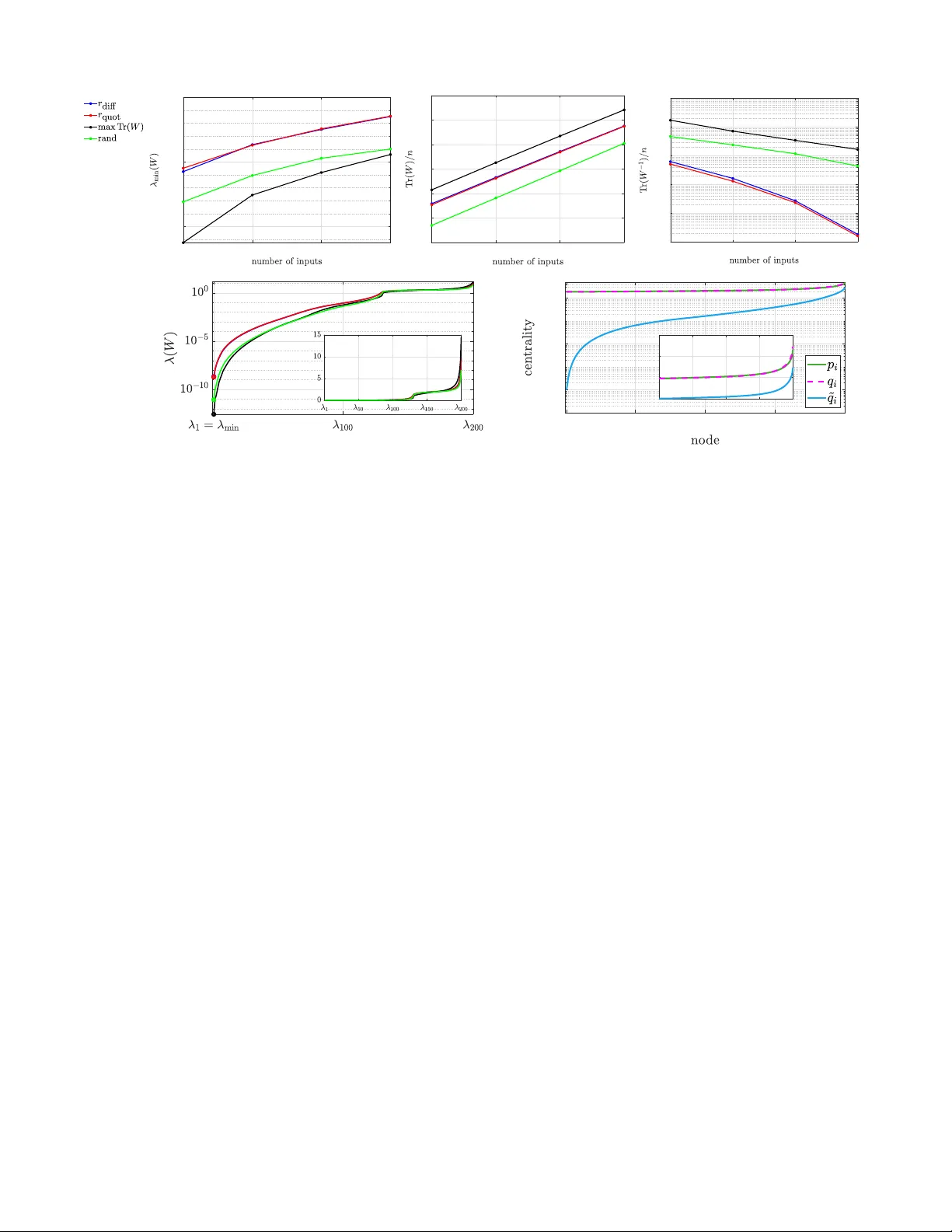
Centrality measures and the role of non-normality for network control ener gy reduction Gustav Lindmark and Claudio Altafini Abstract —Combinations of Gramian-based centrality mea- sures are used for driver node selection in complex networks in order to simultaneously take into account conflicting control energy requir ements, like minimizing the av erage energy needed to steer the state in any direction and the energy needed for the worst dir ection. The selection strategies that we pr opose ar e based on a characterization of the network non-normality , a concept we show is related to the idea of balanced r ealization. I . I N T RO D U C T I O N In recent years, there has been a renewed interest in the controllability problem, motiv ated by its application in the context of complex networks. Depending on the context, many are the possible ways to define control inputs on networks, from drugs in biological networks [2] to dams in irrigation networks, from traffic lights in intersections to opinion makers in social networks, etc. Given a network, deciding where to place the controls is often an inte gral part of the controllability problem. In the ideal case, a control can be placed on any node of the network, hence it is of interest to provide criteria for driver node placement that guarantee controllability . The notion of structural controllability [3] has proven to be very useful to determine where to place a minimal number of driv er nodes that achiev e controllability ([4], [5] and others). Howe ver , a network may be controllable in theory but not in practice if for instance unreasonable amounts of control energy are required to steer it in some direction. For linear dynamics, the measures of control ener gy are normally formulated in terms of the controllability Gramian [6]. Sev eral of the papers that hav e appeared in recent years on the subject in fact rely on properties of the Gramian. For instance [7], [8] quantify the importance of the dif ferent nodes for controllability using Gramian-based network centrality measures. Optimization- based approaches are instead used in [9], [10]. None of these approaches has pro ven valid in all situations, especially because different measures of control energy correspond to different centrality measures and hence to dif ferent driv er node selections criteria. In [11], we showed numerically that the energy required to control a network is influenced by a connectivity property expressed as a ratio between the weighted outdegree and indegree of the nodes. In this paper, the empirical results of [11] are put into a more solid formal basis, and interpreted in terms of the algebraic properties of the adjacency matrix of the netw ork. Our main result is to propose two strategies A preliminary version of this paper was be presented at ECC’19, [1]. G. Lindmark and C. Altafini are with the Division of Automatic Control, Dept. of Electrical Engineering, Link ¨ oping Univ ersity , SE- 58183, Link ¨ oping, Sweden. email: gustav.lindmark@liu.se, claudio.altafini@liu.se for driver node placement, based on a no vel characterization of network non-normality as imbalance in the distribution of energy in the network. W e establish an equiv alence between a network with normal adjacency matrix and a system with balanced realization [12]. Our formulation allo ws to quantify network non-normality at a node lev el as combinations of two different centrality metrics. The first measure ( node-to-network centrality) quantifies the influence that each node has on the rest of the network. It corresponds to the energy with which the node excites the network. The second measure ( network-to- node centrality) describes instead the ability to control a node indirectly from the other nodes, and corresponds to the energy that reaches the node from the other nodes. Suggesti vely , this centrality is formulated in terms of the observability Gramian, and it is somewhat related to structural controllability , as it identifies the nodes that cannot be controlled indirectly and hence must be driv er nodes. W e sho w that the tw o centralities can be expressed as special cases of the H 2 system norm, and can be formally related to performance bounds on some of the most commonly used control energy metrics. These results suggest that nodes with a high node-to-network centrality (i.e., with a high network influence) and nodes with a low network-to-node centrality (i.e., nodes that are difficult to control indirectly) should be driv er nodes, and the strategies for driver node placement that we propose combine the centralities in such a direction. Practically , the strategies consist in selecting the nodes that maximize the network non-normality . In this way we achieve good performances both in terms of the a verage ener gy that is required to steer the network and in terms of the energy required to steer it in the most difficult direction. The rest of the paper is organized as follows: In Section II, definitions are giv en, results on controllability are revised and dif ferent energy-related metrics are discussed. In Section III, the network centralities are presented and their formal relations to the control energy metrics are deriv ed. Section IV is about netw ork non-normality and balanced systems, while in Section V the driv er node placement strategies are presented. A preliminary version of this paper was presented at ECC’19 [1]. This conference paper discusses the network centralities for discrete-time systems. Results such as Theorem III.3 and, most importantly , the material of Section IV are howe ver presented here for the first time. I I . B A C K G RO U N D A. Notation W e denote R n × m the set of n × m matrices with real valued entries. The k -th v ector of the canonical basis of R n is denoted e k , k ∈ 1 , . . . , n . For the vector z ∈ R n , k z k = √ z > z is its Euclidean norm . Giv en a matrix M ∈ R n × m , let M [ k ] = M e k , k ∈ 1 , . . . , m, denote the k -th column of M and M ij = e > i M e j , i ∈ 1 , . . . , n , j ∈ 1 , . . . , m, the element on row i and column j . For M ∈ R n × n , diag ( M ) ∈ R n is the vector of its diagonal entries. Giv en two matrices M , N ∈ R n × n , [ M , N ] = M N − N M is their matrix commutator . A matrix A is said normal if [ A, A > ] = 0 , non-normal otherwise. Gi ven a vector z ∈ R n , the nonincreasing rearrangement of z is the vector z ↓ ∈ R n whose entries are the same as those of z (including multiplicities) b ut rearranged in nonincreasing order z ↓ 1 ≥ · · · ≥ z ↓ n . A (directed) graph G is indicated by the pair of its nodes and edges, V = { v 1 , . . . , v n } and E = { ( v i , v j ) , i, j ∈ 1 , . . . , n } , or , if it is necessary to specify the edge weights, by the adja- cency matrix A , i.e., G = G ( A ) . Then the weight associated with the edge from v i to v j , ( v i , v j ) , is A j i . The node v i ∈ V is a root if it has no incoming edge and a leaf if it has no outgoing edge. B. Contr ollability W e consider the following continuous-time linear time- in v ariant model for the network ˙ x ( t ) = Ax ( t ) + B K u ( t ) , (1) where x ( t ) ∈ R n is the state at time t ≥ 0 , A ∈ R n × n , B K = [ e k 1 . . . e k m ] ∈ R n × m and u ( t ) ∈ R m . W e represent the network with the directed graph G ( A ) = ( V , E ) . Each control input is assumed to act on only one node which is then called a driver node . The set of driver nodes is K = { v k 1 , . . . , v k m } ⊆ V . The system (1) is controllable if and only if the controllability Gramian W ( t f ) = Z t f 0 e At B K B > K e A > t dt, (2) is positive definite. For A stable, the controllability Gramian con ver ges as t f → ∞ . W e omit the dependency on t f in the following. The minimal energy that is needed to steer the network in a specific direction of the state space can be exactly computed from the controllability Gramian. When all directions are considered, the following metrics for the control energy are commonly used: i) The minimal eigen value of W , λ min ( W ) : The energy required to steer the system in the worst case direction is 1 /λ min ( W ) . ii) T r( W − 1 ) : The trace of the in verse Gramian is propor- tional to the av erage energy required to control a system ov er all directions of the state space. iii) T r( W ) : The trace of the Gramian is inv ersely related to the a verage energy required to control a system. See e.g. [6], [9] for more details about the dif ferent control energy metrics. For a stable linear input-output system H with system matrices ( A, B , C ) , the H 2 norm can be computed from the (infinite horizon) controllability Gramian, k H k 2 2 = T r( C W C T ) . (3) I I I . C E N T R A L I T Y M E A S U R E S F O R T H E C O N T R OL E N E R G Y W e begin this section by defining a quantity we call walk ener gy , which we use to deri ve the proposed centrality mea- sures. Following that, we relate them to the considered control energy metrics. A. Centrality measur es W e define the walk ener gy from v i to v j as ε i → j = Z t f 0  ( e At ) j i  2 dt. (4) This is in fact the squared H 2 norm of the system A , B = e i , C = e > j , and can be thought of as the excitation energy of node v j when a unit impulse is applied to node v i . Let W ( i ) = Z t f 0 e At e i e > i e A > t dt, i = 1 , . . . , n, (5) i.e. the Gramian when v i is the only driver node. For the diag- onal elements in (5) we hav e  W ( i )  j j = ε i → j , j = 1 , . . . , n . W ith the driver nodes K = { v k 1 , . . . , v k m } the controllability Gramian (2) can be written W = X i = k 1 ,...,k m W ( i ) , (6) see e.g. [7] for a deri vation. In particular , the diagonal elements W j j = X i = k 1 ,...,k m ε i → j , j = 1 , . . . , n. (7) For A stable the w alk ener gies con verge as t f → ∞ . Definition III.1. The node-to-network centrality p i is the total walk ener gy fr om v i to all nodes, p i = n X j =1 ε i → j = T r( W ( i ) ) . (8) Equation (8) is the same as the squared H 2 norm (3) with C = I and W = W ( i ) , hence we can interpret it as the energy injected into the system ( C = I means all nodes) by v i . W e use the centrality p i for quantifying the network impact of v i as a driver node. Equation (6) and the linearity of the trace operator gi ves T r( W ) = X i = k 1 ,...,k m p i . (9) The centrality p = { p 1 , . . . , p n } appears also in [9] where the dri ver node placement problem is in vestigated using opti- mization techniques. From (9), for m a given number of dri ver nodes, the control energy metric T r( W ) is maximized when K is the set of the m nodes with highest p i . Howe ver , driv er node placement based on p alone does not e ven guarantee control- lability , as worst-case directions requiring infinite energy may still e xist. For instance, the p centrality does not f av our roots ov er other nodes, although controllability is never achiev ed unless all roots are dri ver nodes. Introduce the fictitious output equation y ( t ) = C x ( t ) , where y ( t ) ∈ R d is the output at time t and C ∈ R d × n . The observability Gramian M ( t f ) = Z t f 0 e A > t C > C e At dt is positiv e semidefinite and conv erges as t f → ∞ for A stable. The dependency on t f is omitted in the following. In analogy with W ( i ) , i = 1 , . . . n , introduce M ( j ) = Z t f 0 e A > t e j e > j e At dt, j = 1 , . . . , n, i.e. the observ ability Gramian with the state of v j as the only output. The diagonal elements are M ( j ) ii = ε i → j , v i , v j ∈ V . W e use the sum of the walk energies to v j from all the other nodes as a metric for the ability to control v j indirectly , ˜ q j = X ∀ i 6 = j ε i → j . (10) From the definition of walk energy we obtain ˜ q j ≥ 0 , j ∈ 1 , . . . , n . The metric attains its least value ˜ q j = 0 if and only if v j is a root. Furthermore, it is close to its minimum for nodes with only fe w and weak incoming edges, i.e. “almost” root nodes. Besides ˜ q j , we will also use the following centrality metric. Definition III.2. The network-to-node centrality q i is the total walk ener gy fr om all nodes to v j , q j = n X i =1 ε i → j = T r( M ( j ) ) . (11) The centrality q j is the squared H 2 norm of the system ( A, B = I , C = e > j ) , hence interpretable as the system energy that a impulse input at each node injects into node v j . Since q j = ˜ q j + ε j → j with ε j → j > 0 , it is q j > 0 . B. Contr ol ener gy bounds Lemma III.1 below follo ws directly from (7) and the defi- nitions of q and ˜ q . The result is later used to deri ve theoretical bounds relating the control energy metrics λ min ( W ) and T r( W − 1 ) to the centrality measures (Theorems III.2 and III.3 respectiv ely). Lemma III.1. The diagonal elements W j j , j = 1 , . . . , n, ar e bounded by (i) W j j = q j if K = V (the network is fully actuated), (ii) 0 ≤ W j j ≤ ˜ q j if v j ∈ V \ K , and (iii) ε j → j ≤ W j j ≤ q j if v j ∈ K . Theorem III.2. W ith K a set of driver nodes, it holds λ min ( W ) ≤ min { q i , ˜ q j } , i = 1 , . . . , n, and j s.t. v j ∈ V \ K . Pr oof. Since W is symmetric, λ min ( W ) = min k x k =1 x > W x ≤ e > j W e j = W j j , j = 1 , . . . , n. The result of the theorem is obtained when this is used with properties (ii) and (iii) of Lemma III.1. Notice that λ min ( W ) ≤ q i , i = 1 , . . . , n, holds for any K ⊆ V . In the following corollary , let the indices j 1 , . . . , j n be such that ˜ q j 1 ≤ ˜ q j 2 ≤ · · · ≤ ˜ q j n . Corollary III.2.1. F or any set K of m driver nodes, the minimal eigen value of the Gramian is bounded by λ min ( W ) ≤ min { q i , ˜ q j m +1 } , i = 1 , . . . , n. (12) Pr oof. T aking K in Theorem III.2 as the set of nodes with lowest ˜ q j giv es the bound (12). For any other K s.t. |K| = m < n ∃ d ∈ 1 , . . . , m s.t. v j d ∈ V \ K and λ min ( W ) ≤ ˜ q j d ≤ ˜ q j m +1 . As a consequence of Corollary III.2.1, the nodes with the lowest ˜ q and q giv e a direct upper bound on λ min ( W ) , i.e. a lower bound on the energy required to control the network in the most difficult direction. Theorem III.3. F or any set of driver nodes K suc h that the network is controllable it holds T r( W − 1 ) ≥ X j s.t. v j ∈K 1 q j + X j s.t. v j ∈V \K 1 ˜ q j . (13) Pr oof. Since W is symmetric, by the Schur-Horn theorem for Hermitian matrices [13], the vector of eigenv alues λ ( W ) = [ λ 1 ( W ) . . . λ n ( W )] > majorizes diag( W ) , i.e., k X i =1 λ i ( W ) ↓ ≥ k X i =1 diag i ( W ) ↓ for each k = 1 , 2 , . . . , n , with equality for k = n . Applying Hardy-Littlew ood-P ´ olya’ s inequality on majorizing sets and con ve x functions [14] to λ ( W ) and diag( W ) gives n X i =1 1 λ i ( W ) ≥ n X i =1 1 W ii . Controllability implies that V \ K contains no root nodes (all root nodes must be driv er nodes). Hence, ˜ q j > 0 ∀ j s.t. v j ∈ V \ K and the bound (13) exists. By Lemma III.1, 1 /W j j ≥ 1 /q j if v j ∈ K and 1 /W j j ≥ 1 / ˜ q j otherwise. Hence, T r( W − 1 ) = n X i =1 1 λ i ( W ) ≥ n X j =1 1 W j j ≥ X j ∈K 1 q j + X j ∈V \K 1 ˜ q j . Since q j ≥ ˜ q j + ε j → j , the second sum in (13) is the most important. Nodes with low ˜ q that are not dri ver nodes result in the lower bound (13) being high. As a corollary of Theorem III.3 we obtain a lower bound on T r( W − 1 ) for a giv en number of dri ver nodes. Corollary III.3.1. Assume contr ollability . W ith the number of driver nodes |K | = m it holds T r( W − 1 ) ≥ m X j =1 1 q ↓ j + n − m X j =1 1 ˜ q ↓ j . (14) A necessary but not sufficient condition for equality in (14) is that K ar e the nodes with the lowest ˜ q j . Pr oof. In Theorem III.3, use the fact that X j s.t. v j ∈K 1 q j ≥ m X j =1 1 q ↓ j , X j s.t. v j ∈V \K 1 ˜ q j ≥ ( n − m ) X j =1 1 ˜ q ↓ j , with equality if and only if K are the nodes with lo west ˜ q j . I V . N O N - N O R M A L I T Y A N D B A L A N C E D S Y S T E M S The notion of balanced realization has a central role in classical control theory and is mainly used for model reduction [12]. Here, we show that the network non-normality can be understood as imbalances in the distribution of energy in the network realization. Moreover , as we quantify these imbalances, the centralities p and q naturally appear . For simplicity , in this section we only consider infinite time horizon controllability and observability Gramians. A. Characterization of network non-normality The follo wing definition can be found in e.g. [12]. Definition IV .1. A contr ol system ( A, B , C ) is balanced if W = M . In a balanced system, the states which are dif ficult to reach are simultaneously difficult to observe. If we assume a fully actuated network where the state of each node is considered an output (i.e. B = C = I ), then any balance/imbalance is entirely due to the weighted adjacency matrix A . As a matter of fact, in this case the notion of balance can be linked to the non-normality of the adjacency matrix. Denote by W ( V ) , M ( V ) the controllability and observability Gramians corresponding to B = C = I . Theorem IV .1. A stable, fully actuated and observed network is balanced if and only if the weighted adjacency matrix A is normal. Pr oof. W ( V ) and M ( V ) are the solutions to the L yapunov equations A > W ( V ) + W ( V ) A + I = 0 , M ( V ) A > + A > M ( V ) + I = 0 . Giv en that A is Hurwiz stable, according to Theorem 2 of [15] it holds that W ( V ) = M ( V ) if and only if A is normal. For instance undirected networks correspond to normal weighted adjacenc y matrices, hence they are balanced. It follo ws from Theorem IV .1 that the matrix N = M ( V ) − W ( V ) = Z ∞ 0 [ e At , e A > t ] dt expresses the non-normality of the network. Such quantity is not in v ariant to a change of basis. In particular , it is well- known [12] that for any controllable and observ able system there e xists a state transformation matrix Q such that ˜ W = Q T W Q = Q − 1 M ( Q − 1 ) > = ˜ M , (15) i.e. the system is balanced in the new basis. When balancing is used for model reduction, it is also required that the two Gramians are diagonal. Howe ver , a change of basis leading to diagonal Gramians will in general destroy the correspondence between the elements of the state vector and the nodes, i.e. between the A matrix and the network topology . For irreducible A , only a diagonal state transformation matrix preserves the topological/algebraic cor- respondence, as it amounts to rescaling the states of the nodes while not mixing states at dif ferent nodes. B. Non-normality in a node In case N 6 = 0 , we say that z > N z is the non-normality in direction z ∈ R n , || z || = 1 . In particular , we can denote r diff ,i = e > i N e i = M ( V ) ii − W ( V ) ii ∈ R the non-normality corresponding to node v i ∈ V . If r diff ,i = 0 then the node v i is “balanced” (in the sense that it is as dif ficult to control as to observe). While balancing (i.e. ˜ W = ˜ M ) cannot in general be achiev ed with Q diagonal, there alw ays exists a unique positi ve vector , denote it r quot ∈ R n such that Q = diag ( r quot ) achiev es diag ( ˜ M ( V ) ) = diag( ˜ W ( V ) ) , i.e. the diagonal part of ˜ N = ˜ M ( V ) − ˜ W ( V ) is canceled. This means that the node non- normality of v i is canceled by the rescaling ˜ x i = x i /r quot ,i , i ∈ 1 , . . . , n . Also r quot ,i provides a relati ve measure of node non-normality (with r quot ,i = 1 corresponding to v i balanced). Both r diff and r quot are related to our network centralities: Theorem IV .2. The node non-normalities r diff ,i and r quot ,i can be expr essed as r diff ,i = p i − q i and r quot ,i = ( p i /q i ) 1 / 4 , i ∈ 1 , . . . , n . Pr oof. r diff ,i : Using the c yclic property of the trace operator , it can be shown that M ( V ) ii = T r W ( i ) , e.g. the centrality p i , i = 1 , . . . , n . In the same way , W ( V ) ii = q i . Hence, r diff ,i = p i − q i . r quot ,i : Giv en the condition ˜ M ( V ) ii = ˜ W ( V ) ii ∀ i = 1 , . . . , n . W ith Q = diag( r quot ) we obtain ˜ W ( V ) ii = q i r 2 quot ,i and ˜ M ( V ) ii = p i /r 2 quot ,i , hence ˜ M ( V ) ii = ˜ W ( V ) ii ⇔ r 4 quot ,i = p i /q i with r quot ,i = ( p i /q i ) 1 / 4 the only positive real root. Notice that P n i =1 r diff ,i = 0 , meaning that if some nodes hav e a positiv e non-normality then others must hav e a negati ve non-normality . C. Non-normality in a set of nodes The node non-normalities r diff ,i and r quot ,i can be combined for sets of nodes. For S ⊆ V , let r diff , S = X i s.t. v i ∈S e > i N e i = X i s.t. v i ∈S r diff ,i (16) be the non-normality of the node set S . Giv en two sets of nodes S 1 ⊆ V and S 2 ⊆ V , define the net walk energy from S 1 to S 2 as ∆ ε S 1 →S 2 = ε S 1 →S 2 − ε S 2 →S 1 = X i s.t. v i ∈S 1 j s.t. v j ∈S 2 ( ε i → j − ε j → i ) . Proposition 1. F or S ⊆ V , the node set non-normality r diff , S is the net walk ener gy fr om S to V \ S . The proposition follows from straight-forward manipula- tions of (16). In the ne xt section we will use the node set non-normality for driver node placement, i.e. for determining the set K . Since r diff , K is a linear function of the set K (equation (16)), for a given |K | = m , it is maximal when K is the set of m nodes with highest r diff ,i . When m is left arbitrary , (16) implies that the maximal node set non-normality is giv en in correspondence of K = { v i , i s.t. r diff ,i ≥ 0 } . This case describes how to partition the nodes into the two sets K and V \ K that achieve the maximum net walk energy from the former to the latter . For the generalization of r quot ,i to sets of nodes, we seek a common rescaling ˜ x i = x i /r quot , S , ∀ i ∈ S , such that Y i s.t. v i ∈S ˜ M ( V ) ii = Y i s.t. v i ∈S ˜ W ( V ) ii . This is achieved for r quot , S the geometric average of r quot ,i , i s.t. v i ∈ S . Hence, for a gi ven |K | = m , r quot , K is maximal when K is the set of m nodes with highest r quot ,i . V . D R I V E R N O D E P L A C E M E N T W e use the node non-normalities r diff ,i and r quot ,i to rank the nodes for driv er node placement. For a given |K| = m , this means to select the set K ⊆ V that maximizes the node set non-normality r diff , K or r quot , K . Figure 1 shows a small network example with p i , q i , r diff ,i and r quot ,i presented for each node. In our ranking strategies, maximization of p i − q i or p i /q i corresponds to two different trade-offs between nodes produc- ing the largest injection of energy in the system ( max i p i ) and those relying on the least injected energy ( min i q i ). In fact, max i ( p i ) alone corresponds to maximizing T r( W ) but could correspond to ellipsoids of W which are “squeezed” to 0 in certain directions i.e., to infinite energy required along certain eigenspaces of 1 /W (see example in Fig. 1). On the contrary , max i ( − q i ) = min i ( q i ) alone means focusing on nodes that hav e no or little incoming walk ener gy . According to Theorems III.2 and III.3 and their corollaries, these nodes should be driv er nodes in order to improve λ min ( W ) and T r( W − 1 ) . Observe that for a balanced network (with normal weighted adjacency matrix), p = q , r diff = 0 and r quot = 1 for all nodes, hence the rankings are degenerate. Put differently , the best driv er nodes considering the p centrality are the worst nodes considering the q centrality . A. Simulations In [11], a v ariant of r quot was used for dri ver node placement in extensi ve simulation studies. Here, we complement these studies with an in vestigation of the amount of energy that is required to control random networks when r diff and r quot are used for dri ver node placement. F or comparison, we also compute the different control energy metrics for a random driv er node placement and for the placement of driver nodes that maximize T r( W ) . The results are presented in Figure 2. 1 2 3 4 5 6 0.7 0.7 0.05 0.05 0.7 0.7 0.7 0.7 0.7 0.7 0.7 0.7 0.3 0.3 0.3 0.3 Node p q r diff r quot 1 0.76 0.50 0.26 1.52 2 0.82 0.71 0.11 1.15 3 0.64 0.501 0.14 1.27 4 0.90 0.73 0.17 1.23 5 0.53 0.86 -0.33 0.62 6 0.57 0.91 -0.34 0.63 K T r( W ) λ min ( W ) T r( W − 1 ) K tr = { 2 , 4 } 1.72 0 - K diff = { 1 , 4 } 1.66 3 . 84 · 10 − 5 2 . 80 · 10 4 K quot = { 1 , 3 } 1.39 1 . 11 · 10 − 3 1 . 04 · 10 3 Fig. 1. A directed network with 6 nodes. All nodes have self-loops of weight − 1 that are omitted in the figure. With m = 2 the two rankings suggest different sets of dri ver nodes, and the solution that maximizes T r( W ) is also different. T r( W ) is maximized with K tr = { 2 , 4 } . Howe ver , this choice of driv er nodes renders the network uncontrollable since the root node v 1 is not a driver node. The two best nodes according to r diff are K diff = { 1 , 4 } (the root node is included). They render the network controllable and T r( W ) is high. Node 3 is “almost” a root, and the r quot ranking places it as number two in importance. The resulting dri ver node placement K quot = { 1 , 3 } gives the best λ min ( W ) and T r( W − 1 ) but the lowest T r( W ) . W e use random directed scale-free networks in our study . They hav e both an indegree distribution and an outdegree distribution that follows power laws. By choosing these in a suitable way , we can obtain networks with lar ge variations in the two network centralities p and q . The model suggested in [16] is used to generate random networks with 200 nodes, indegree distribution P in ( k in ) ∝ k − 3 . 14 in , and outdegree dis- tribution P out ( k out ) ∝ k − 2 . 88 out . The edge weights are sampled from a normal distribution. In order to ensure stability , the eigen v alues of A are shifted into the complex half plane Re { λ i } ≤ − 0 . 1 , ∀ i through the addition of negati ve self loops, A := A − αI . As the focus is on reducing the control energy , controllability is always ensured for all choices of driver nodes by adding edges that guarantee strong connecti vity when needed. In comparison with randomly placed dri ver nodes, all met- rics improve significantly when the driv er nodes are placed according to r diff or r quot ; the metrics λ min ( W ) and T r( W − 1 ) improv e sev eral orders of magnitude. These results are coher- ent with what is obtained in [11]. Note that the driv er nodes that maximize T r( W ) result in poor values of λ min ( W ) and T r( W − 1 ) , even worse than for a random choice of dri ver nodes for this class of networks. Figure 2(b) shows all the eigen v alues of W (in increasing order) for m = 70 driv er nodes chosen according to the four criteria described abov e. Here λ min ( W ) is the leftmost eigen v alue of each curve. The metrics p , q and ˜ q are shown in Figure 2(c). In f act, choosing power laws for the degree distributions means that the amount of non-normality of the corresponding adjacency matrix is large, as a significant fraction of ov erall outgoing edge weights is concentrated at a fe w nodes, and similarly for the ov erall incoming edge weights, thereby resulting into skewed distri- bution of p i and q i , see Figure 2(c). Corresponding results for discrete time Erd ˝ os-R ´ enyi and directed scale free networks 60 70 80 90 10 -15 10 -10 10 -5 60 70 80 90 0.6 0.7 0.8 0.9 1 1.1 1.2 60 70 80 90 10 11 10 12 10 13 10 14 10 15 10 16 (a) (b) 1 50 100 150 200 10 -4 10 -2 10 0 1 50 100 150 200 0 2 4 6 (c) Fig. 2. Simulation results for random directed scale-free networks with 200 nodes. All displayed values are the averages over 1000 network realizations. (a): Control energy metrics computed for different numbers of driv er nodes. Driv er nodes are selected based on the proposed strategies. (b): The eigenv alues of W in increasing order for different ranking criteria in logarithmic and linear scale (inset). The number of driver nodes is here 70. (c): The metrics p i , q i and ˜ q i in logarithmic and linear scale (inset). The values are sorted in ascending order along the x-axis. that are presented in [1] show that the improv ements with r diff and r quot are smaller for Erd ˝ os-R ´ enyi networks since their adjacency matrices hav e a lo wer degree of non-normality . V I . C O N C L U S I O N S The network centrality measures p and q considered in this paper are based on system energy considerations. They reflect the fact that what mak es a good driver node depends both on its influence over other nodes in the network, and on its ability to be controlled indirectly from other nodes. These centralities are strictly related to the non-normality of the network that can be associated to the nodes. Network non-normality can be understood as imbalances in the distribution of energy in the network. F or a single node it can be quantified by the differ- ence p − q or by the quotient p/q . A driver node placement strategy that maximize the non-normality results in reduced energy requirements for controlling the network, i.e. all the metrics λ min ( W ) , T r( W − 1 ) and T r( W ) are simultaneously improv ed w .r .t. random driver node placement, although none of them is optimized. The improvements are significant for networks which ha ve skewed in- and out-degree distributions, for which the amount of non-normality is non-negligible. R E F E R E N C E S [1] Gustav Lindmark and Claudio Altafini. Combining centrality measures for control ener gy reduction in netw ork controllability problems. In 2019 18th Eur opean Contr ol Confer ence (ECC) , pages 1518–1523. IEEE, 2019. [2] N ´ uria Ballber T orres and Claudio Altafini. Drug combinatorics and side effect estimation on the signed human drug-target network. BMC Systems Biology , 10(1):74, Aug 2016. [3] Ching T ai Lin. Structural controllability . IEEE T ransactions on Automatic Contr ol , 19(3):201–208, 1974. [4] A. Olshevsky . Minimal controllability problems. IEEE T ransactions on Contr ol of Network Systems , 1(3):249–258, Sept 2014. [5] Christian Commault and Jean-Michel Dion. Input addition and leader selection for the controllability of graph-based systems. Automatica , 49(11):3322 – 3328, 2013. [6] P .C. M ¨ uller and H.I. W eber . Analysis and optimization of certain qual- ities of controllability and observ ability for linear dynamical systems. Automatica , 8(3):237 – 246, 1972. [7] Fabio Pasqualetti, Sandro Zampieri, and Francesco Bullo. Controlla- bility metrics, limitations and algorithms for complex networks. IEEE T ransactions on Contr ol of Network Systems , 1(1):40–52, 2014. [8] Nicoletta Bof, Giacomo Baggio, and Sandro Zampieri. On the role of network centrality in the controllability of complex networks. IEEE T ransactions on Contr ol of Network Systems , 4(3):643–653, 2017. [9] T yler H Summers, Fabrizio L Cortesi, and John L ygeros. On sub- modularity and controllability in complex dynamical networks. IEEE T ransactions on Contr ol of Network Systems , 3(1):91–101, 2016. [10] V asileios Tzoumas, Mohammad Amin Rahimian, George J Pappas, and Ali Jadbabaie. Minimal actuator placement with bounds on control effort. IEEE T ransactions on Contr ol of Network Systems , 3(1):67–78, 2016. [11] Gustav Lindmark and Claudio Altafini. Minimum energy control for complex networks. Scientific Reports , 8(1):3188, 2018. [12] Bruce Moore. Principal component analysis in linear systems: Con- trollability , observability , and model reduction. IEEE transactions on automatic control , 26(1):17–32, 1981. [13] Roger A Horn and Charles R Johnson. Matrix analysis . Cambridge univ ersity press, New Y ork, 2012. [14] Albert W Marshall, Ingram Olkin, and Barry C Arnold. Inequalities: theory of majorization and its applications , volume 143. Springer , 1979. [15] George Phillip Barker . Normal matrices and the lyapunov equation. SIAM Journal on Applied Mathematics , 26(1), 1974. [16] B ´ ela Bollob ´ as, Christian Borgs, Jennifer Chayes, and Oliver Riordan. Directed scale-free graphs. In Pr oceedings of the fourteenth annual ACM-SIAM symposium on Discrete algorithms . Society for Industrial and Applied Mathematics, 2003.