Real-Time Predictive Control for Precision Machining

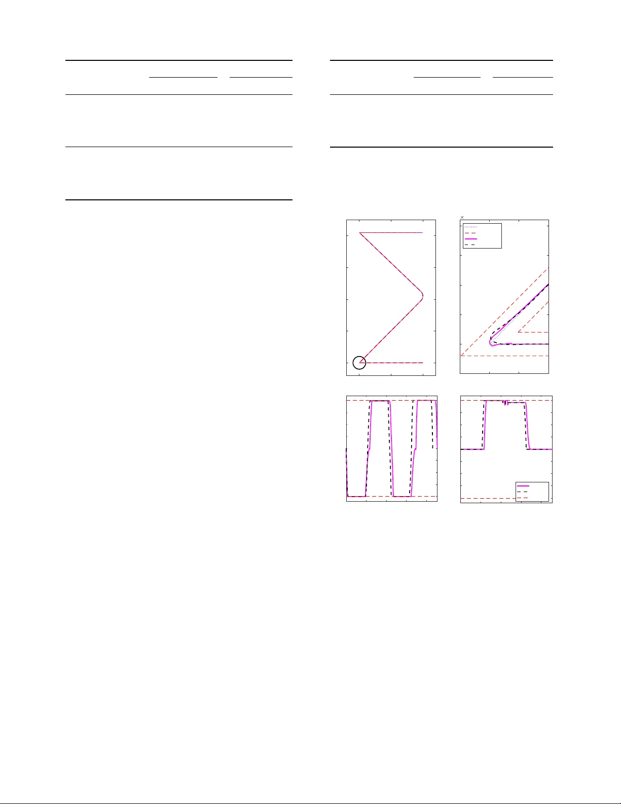
Real-T ime Predicti ve Control for Precision Machining Alexander Liniger , Luca V arano, Alisa Rupenyan and John L ygeros Abstract — Precise positioning and fast traversal times are crucial in achieving high productivity and scale in machining. This paper compar es two optimization-based pr edictive con- trol approaches that achieve high performance. In the first approach, the contour error is defined using the global position, the position on the path is inferred through a virtual path parameter , and the cost function combines the corresponding states and inputs to achieve a trade-off between high speed and positioning accuracy . The second appr oach is based on a local definition of both the error and the progr ess along the path, and results in a system with a reduced number of states and inputs that enables real-time optimization. T erminal and trust region constraints are required to achieve precise tracking of geometries where a fast or instantaneous change in direction is present. The performance of both approaches using different quadratic programming solvers is ev aluated in simulations f or geometries that are challenging in machine tools applications. I . I N T RO D U C T I O N Machine tool control of multi-axis systems is focused on accurate, high-speed tracking of a geometrical path [1]–[3]. The requirement for maximum producti vity combined with high precision in contouring applications is reminiscent to the challenges encountered in autonomous race driving [4], [5]. In high-precision cutting, the driv er is the tool head, the lane width is the machining tolerance, and the optimized trajec- tory is the cutting contour . Similar methodology to generate a time-optimal trajectory can be applied, with the emphasis on tight tolerances in the order of tens of micrometers. Model Predictiv e Contouring Control (MPCC) methods hav e been proposed to increase the productivity of multi-axis computer numerical control (CNC) machine tools as they enable the coupled optimization of the velocity (feed) and the position of the tool. In [1] the contour, defined as the desired geometry to be tra versed, is parametrized using the arc-length of the reference path. Based on the formulation presented in [6], where the cost function couples the contouring error with the progression on the geometrical path, a non-linear Model Predictiv e Control (MPC) formulation is proposed which trades off the contouring error and the trav ersal speed. The resulting non-linear MPC problem is solved by linearizing each segment, thus allowing to conv ert the problem into a quadratic program (QP). MPCC accounts for the real behavior of the machine and the axis drive dynamics can be excited to compensate for the contour error to a big extent, even without including friction effects in the model [2], [7]. High-precision trajectories or set points can be generated prior to the actual machining process The authors are with the Automatic Control Laboratory , ETH Z ¨ urich, 8092 Z ¨ urich, Switzerland. A. Rupenyan is also with inspire AG, 8092 Z ¨ urich, Switzerland. (e-mails: { liniger,ralisa,lygeros } @control.ee.ethz.ch) following various optimization methods, including MPC, feed-forward PID control strategies, or iterativ e-learning con- trol [8], [9], where friction or vibration-induced disturbances can be corrected. T o achiev e real-time performance with MPC, combined with accounting for persistent disturbances, the contouring error can be reduced by modifying the ref- erence geometry of fline based on the predicted contouring error [10]. This work demonstrates two contouring control ap- proaches, using MPC methods with a linear time-varying formulation. A modification of the MPCC method applied to biaxial machine tools as implemented in [1] and [11] is compared with a local-variable method used in path following for autonomous driving and racing [4], [12]–[14]. The two approaches differ in the definition of the contour- tracking error and how they tie it with the path. In the first approach the error is coupled with the progression along the path through the cost function. In the second approach the error is a component of the local coordinate transformation of the position along the path and the error progression is thus directly coupled to the system dynamics. The numerical implementation demonstrates on a simplified system exclud- ing friction and oscillations that contour-tracking problems can be solved with a sampling rate in the order of 1 ms, making the methods suitable for real-time implementation. I I . P RO B L E M D E FI N I T I O N In this paper we look at a biaxial machine tool contouring control problem, where the goal is to trav erse a given geom- etry as fast as possible while staying within a giv en tolerance band. W e model the machine as a lumped mass model where the acceleration in X - Y can be controlled individually . The resulting model is a classical double integrator model with the states given by x = ( X, Y , v x , v y ) and the inputs giv en by u = ( a x , a y ) . The linear continuous time model can then be exactly discretized using periodic sampling and a Zero Order Hold (ZOH). The machine has independent acceleration limitations in the X - Y direction of ± 20 m/s 2 , resulting in the input constraints u ∈ U = { u x , u y | | u x | ≤ 20 m/s 2 , | u y | ≤ 20 m/s 2 } . The velocity components v x , v y are limited to ± 0 . 2 m/s, and the velocity constraints are defined as v ∈ V = { v x , v y | | v x | ≤ 0 . 2 m/s , | v y | ≤ 0 . 2 m/s } . The geometry which should be traversed with the tool is parametrized by the arc-length of the curve s ∈ [0 , L ] as path parameter: r d ( s ) = ( r d,x ( s ) , r d,y ( s )) . In our case the contour is gi ven as piecewise linear in s , thus, the deriv ati ve of the geometry with respect to the s can be computed and is giv en by r 0 d ( s ) = ( r 0 d,x ( s ) , r 0 d,y ( s )) which can be interpreted as the tangent at the point r d ( s ) . Note that at the switching points one of the subgradients is used. The geometry also comes with a tolerance band the tool is not allowed to leave, in our case defined as ± 20 µ m perpendicular to the contour . Based on these ingredients we can now formulate the MPC- based contouring control problem. I I I . C O N TO U R I N G C O N T RO L A P P RO AC H E S A. Global variable MPCC The aim of the MPCC of [1] is to minimize the distance between the geometry and the optimized trajectory , while trav ersing the geometry as fast as possible [15]. As dis- cussed in Section II, the geometry is giv en by r d ( s ) and is parametrized by the arc-length of the curve. The optimized trajectory at time k is defined as r d,k = ( X k , Y k ) . A virtual path parameter s k is introduced as s k +1 = s k + T v s,k , where v s,k is the velocity along the path at time step k and T is the sampling time. The idea of the global v ariable MPCC formulation is to use the virtual path parameter s k to approximate the true path parameter ˆ s corresponding to a position r d,k . The dif ference in arc-length between r d ( ˆ s ) and r d ( s k ) is defined as the lag error e l,k , and the distance from r d ( ˆ s ) to r d,k as the contouring error e c,k . Furthermore, the total error r d ( ˆ s ) − r d,k is approximated with r d ( s k ) − r d,k . Fig. 1: Definition of global variable (a) and local variable (b). The resulting error vector is decomposed into a part ˆ e l,k which is parallel to the tangent of the path at s k and another part ˆ e c,k which is perpendicular to the tangent, the errors are defined as follows, ˆ e l,k ( s k ) = r 0 d ( s k ) k r 0 d ( s k ) k · ( r d ( s k ) − r d,k ) (1) ˆ e c,k ( s k ) = r 0 d ⊥ ( s k ) k r 0 d ⊥ ( s k ) k · ( r d ( s k ) − r d,k ) , (2) where the parametric deri vati ve r 0 d is defined as r 0 d ( s ) = ( r 0 d,x ( s ) , r 0 d,y ( s )) and the vector perpendicular to the tangent can be easily calculated as r 0 d ⊥ ( s ) = ( − r 0 d,y ( s ) , r 0 d,x ( s )) . If ˆ e l,k is small, ˆ e c,k is a good approximation of the contour error and the virtual path parameter is a good approximation of ˆ s . The virtual parameter represents the progression on the path which can be controlled with the input v s,k . The connection between the longitudinal error and the path parameter is a key feature of the MPCC which ties the progression on the path with the contour error and is later included into the cost function. The errors as defined in (1) and (2) solely depend on states at time k . Howe ver , fast QP solvers such as the ones used in our simulation study , do only allow for equality constraints linking two consecutiv e time steps. Thus, we reformulate the errors at time step k + 1 to depend only on information of time step k , thus introducing error dynamics. More precisely the error dynamics depends on the state x k and inputs u k of the lumped mass model, as well as on the errors e l,k , e c,k , the virtual path parameter s k , and the velocity along the path v s,k . As a first step the error is linearly approximated along the geometry around s k : ˆ e l,k +1 = r 0 d,x ( s k ) k r 0 ( s k ) k ( r d,x ( s k ) − X k +1 ) + r 0 d,y ( s k ) k r 0 ( s k ) k ( r d,y ( s k ) − Y k +1 ) + T v s,k (3) ˆ e c,k +1 = − r 0 d,y ( s k ) k r 0 ( s k ) k ( r d,x ( s k ) − X k +1 ) + r 0 d,x ( s k ) k r 0 ( s k ) k ( r d,y ( s k ) − Y k +1 ) . (4) The k + 1 terms on the right hand side can be replaced with terms known from the lumped mass dynamics: X k +1 = X k + T v x,k + T 2 / 2 a x,k , Y k +1 = Y k + T v y ,k + T 2 / 2 a y ,k . The resulting larger dynamical system has a state giv en by ˆ x = ( X , Y , v x , v y , s, e l , e c ) and an input ˆ u = ( a x , a y , v s ) , but, due to (3) and (4) the system is no longer linear . The non-linearity comes from the geometry terms r ( s ) and r 0 ( s ) , which are non-linear in s . Since we solve the problem in a receding horizon fashion, we can use the shifted previous solution of the s state as a guess for the solution and linearize the geometry terms around this estimated s trajectory . As long as the solutions between consecutiv e MPC solutions do not differ too much, this approach should result in good approximations of the error dynamics. This linearization results in a linear time varying system of the form ˆ x k +1 = ˆ A k ˆ x k + ˆ B k ˆ u k + ˆ g k , where only the error dynamics are time- dependant. Finally , we design a cost function that matches the goals of the contouring controller . W e include a term penalizing the squared longitudinal error ˆ e 2 l since this error has to be small for the formulation to be accurate, and a term to minimize the squared contouring cost ˆ e 2 c as this represents our goal of following the geometry closely . W e reward progress at the end of the horizon s N , which corresponds to tra versing the geometry as fast as possible, and penalize the squared velocities and applied inputs, to ha ve smooth velocity and input trajectories. The resulting MPCC problem has the following form, min ˆ x , ˆ u N − 1 X k =1 γ l ˆ e 2 l,k + γ c ˆ e 2 c,k + v T k Q v v k + u T k Ru k + γ l,T ˆ e 2 l,N + γ c,T ˆ e 2 c,N + v T N P v v N − γ s s N s.t ˆ x = ˆ x (0) ˆ x k +1 = ˆ A k ˆ x k + ˆ B k ˆ u k + ˆ g k ˆ e c,k ∈ T c , v k ∈ V , u k ∈ U v N ∈ V T , ˆ e c,N ∈ T c T k = 0 , .., N − 1 (5) where ˆ x = ( ˆ x 0 , ..., ˆ x N ) and ˆ u = ( ˆ u 0 , ..., ˆ u N − 1 ) are the state and input trajectories. γ l and γ c are the error weights, Q v and R are positiv e definite velocity and input weight matrices. The terminal cost consists of the lag, contouring, and velocity weights γ l,T , γ c,T and P v , as well as the progress maximization weight γ s . The MPCC problem constrains the contouring error to stay within the tolerance band, which we denote by T c , in addition to the velocity and input constraints mentioned in Section II. Finally , we impose terminal constraints which constrain the velocity to ± 0 . 002 m/s and the contouring error to ± 20 µ m. The terminal cost and constraints are imposed to deal with potentially fast changing geometries not yet “seen” by the MPC, which would otherwise result in recursive feasibility issues. W e discuss the implications of the terminal constraints further in Section III-C. B. Local V ariable Appr oach The global variable approach uses the global position to define the errors and a virtual path parameter to define the position on the path. The error states are recomputed at every time step and are only introduced into the dynamics such that a cost and constraints can be assigned to them, resulting in a system with some redundant states. T o simplify the problem, a second approach is implemented, where a local definition for the error and the progression on the path is used, resulting in a state space system with a reduced number of states and inputs, all having real dynamics. This implementation is inspired by path following controllers in autonomous driving such as the methods proposed in [12]. The idea is to describe the system in a local curvilinear coordinate system, where the local state is formed by the velocities, the path parameter s , and the perpendicular distance from the path to the machine position, which we call d (see Fig 1b). Note that giv en these coordinates and the path, the global coordinates can be reconstructed. The dynamics in this local coordinate system can be formulated giv en the local angle of the path, which is commutable by the parametric deri vati ve r 0 d ( s ) as θ ( s ) = atan2 ( r 0 d,y ( s ) , r 0 d,x ( s )) . The mov ement along the path can then be described through the projection of the horizontal and the vertical velocities on the path, ˙ s = v x cos( θ ( s )) + v y sin( θ ( s )) 1 − κ ( s ) d , (6) where κ ( s ) is the local curvature. For the geometries and tracking errors that arise in this application the denominator in (6) is roughly equal to 1. W e will therefore ignore the dependence on the curv ature in the sequel. T o simplify the notation, we will also drop the dependence of the angle on s and write simply θ in place of θ ( s ) . Similar to the dynamics along the path, the mov ement perpendicular to the path is the projection on the vector perpendicular to the tangent, ˙ d = − v x sin( θ ) + v y cos( θ ) . (7) The resulting state of the system is given by ˜ x = ( v x , v y , s, d ) and the input is again ˜ u = ( a x , a y ) . Following ZOH discretization the system dynamics is giv en by:     v x,k +1 v y ,k +1 s k +1 d k +1     =     1 0 0 0 0 1 0 0 cos( θ ) T sin( θ ) T 1 0 − sin( θ ) T cos( θ ) T 0 1         v x,k v y ,k s k d k     +     T 0 0 T cos( θ ) T 2 / 2 sin( θ ) T 2 / 2 − sin( θ ) T 2 / 2 cos( θ ) T 2 / 2      a x,k a y ,k  . (8) Since the angle θ is a non-linear function of the path parameter s , we again use the solution of the previous MPC problem to linearize these non-linear terms, as in the global variable approach III-A. The resulting cost function only needs a weight to min- imize the de viation from the path d , penalization of the velocities and inputs for smooth trajectories, and a re ward on the path progression s N . Altogether the following local MPC problem can be formulated, min ˜ x , ˜ u N − 1 X k =1 γ d d 2 k + v T k Q v v k + u T k Ru k + γ d,T d 2 N + v T N P v v N − γ s s N s.t ˜ x = ˜ x (0) ˜ x k +1 = ˜ A k ˜ x k + ˜ B k ˜ u k d k ∈ T c , v k ∈ V , u k ∈ U v N ∈ V T , d N ∈ T c T k = 0 , .., N − 1 (9) where, ˜ x = ( ˜ x 0 , ..., ˜ x N ) and ˜ u = ( ˜ u 0 , ..., ˜ u N − 1 ) are the state and input trajectories. γ d is the weight on the deviation from the path, Q v and R are positi ve definite velocity and input weight matrices. Similar to the global MPC problem (5), the terminal cost consists of higher contouring and velocity weights γ d,T and P v , as well as the progress maximization weight γ s . The constraints as well as the terminal constraints are identical to those of the global MPC problem (5), with the only dif ference that the de viation from the path is denoted by d instead of e c . C. Dealing with sharp corners 1) T erminal Ingr edients: The terminal cost and con- straints are of fundamental importance for this application, since the tool should be able to traverse sharp corners that may result in the MPC optimization problem becoming infea- sible. This can be av oided by requiring that the tool has to be able to stop on the reference path at the end of the horizon, as from such a state any subsequent geometry can be traversed. A zero velocity terminal constraint ( v x,N = v y ,N = 0 ) does ev en guarantee recursiv e feasibility of the problem as for both systems this is an equilibrium. In our implementation we use a relax ed version of the constraint as some of the used QP solvers do not allow for zero velocity terminal constraints, where | v x,N | < = 0 . 002 m/s and | v y ,N | < = 0 . 002 m/s, combined with a high terminal quadratic cost on the velocities. The addition of these terminal constraints may result in conservati ve performance for short horizons, as they implicitly limit the maximum velocity to a velocity where the tool can decelerate to a standstill. For longer horizon the influence on the closed loop results becomes negligible. 2) T rust Re gion Constraints: The local MPC formulation model heavily depends on the angles θ ( s ) , howe ver , as the trajectory changes slightly form iteration to iteration, the linearization points for these angles are not completely correct. This can result in large model prediction errors, especially if the tool needs to trav erse corners with small radius ( < 1mm) or sharp corners. Therefore, we impose trust region constraints for s k to force the current solution to remain close to the previous solution. This results in low prediction errors and is essential for successful tra versal of tight corners as presented in the numerical results. The corresponding additional constraints to (9) are of the form s k ≤ s k ≤ s k , where to s k and s k depend on the previous MPC solution. Note that every time step has its own bounds. 3) Local MPCC State F eedbac k: Due to the model mis- match introduced by the changing angle of the geometry changing over one time step, simply simulating the dynamics (8) is not a valid option. This is especially true for sharp corners where the angle changes rapidly (in the limit discon- tinuously). Therefore, we instead simulate the lumped mass model in global coordinates and then project the position onto the path. Since we have a good initial guess for the location of the projection, we can find locally the closest segment of our piecewise linear geometry and then project onto this segment using an inner product. Note that this is not necessary for the global MPCC approach as the system is formulated in global coordinates. I V . R E S U LT S The simulations are executed in Arch Linux on a desk- top PC with an Intel Core i9 9900K CPU. All files are compiled using gcc with the -O3 option enabled. W e ha ve implemented the simulations on acados , an interface to fast and embedded solvers for nonlinear optimal control and dynamic optimization [16], providing a conv enient frame- work to ev aluate various MPC implementations and solver performance. Currently av ailable MPC solvers are qpOASES [17], HPIPM using BLASFEO [18], and HPMPC [19]. In all simulations the system is modelled using the lumped mass double integrator model. The performance of the two MPCC approaches is assessed by the RMS error in tracking of the target geometry , the infinity-norm tracking error, and by the maneuver time (the time needed for the tool to complete the geometry). W e hav e in vestigated the ef fect of modifying the penalty on the contouring error in the cost function which controls the trade-off between tracking accuracy and machining time. The sampling time of the MPC is 1 ms and the horizon length is chosen such that the terminal constraints do not affect the performance. The performance of the two approaches is compared for horizons of 35 and 70 time steps using the HPIPM solver . W e first in vestigate the tracking performance of the two approaches on a smooth geometry , then on a geometry with sharp edges, and finally compare the com- putational performance and the av ailable QP solvers. A. Smooth geometry T o assess the effect of large geometric variations on the performance of the two approaches, we hav e tested the two approaches on two similar paths based on the Greek letter Σ , one with sharp and one with rounded corners. The sigma geometry is 10 cm wide and 20 cm high, for both geometries the middle edge is rounded and has a radius of 1 cm (see Figure 2 and 3). The other two corners are different for the two geometries, where the smooth geometry has rounded corners with a radius of 0.5 mm (see Figure 2), and the geometry with the sharp corners has an instantaneous change in direction (see Figure 3). The weights of both the global and local MPCC were set to be equal to compare the results, and only the contouring error weight and the horizon length were changed. Figure -0.1 -0.05 0 X [m] 0 0.05 0.1 0.15 0.2 Y [m] -0.1005 -0.1 -0.0995 X [m] -2 0 2 4 6 8 10 12 14 16 Y [m] 10 -4 Geometry Bounds Global Local 0 0.5 1 1.5 2 t [s] -0.2 -0.15 -0.1 -0.05 0 0.05 0.1 0.15 0.2 v x [m/s] 0 0.5 1 1.5 2 t [s] -0.2 -0.15 -0.1 -0.05 0 0.05 0.1 0.15 0.2 v y [m/s] Global Local Bounds Fig. 2: Experimental results for the smooth geometry using long horizon and high contouring cost. 2 shows the e xperimental results for the geometry with rounded corners with long horizon length and high contour- ing cost, and T able I summarizes the tracking error (root mean square (RMS)-tracking and infinity-norm tracking) and the maneuver time for each combination of contouring cost and horizon length. For the high contouring cost case ( γ c = γ d = 10 8 ), the tracking error increases for long horizon lengths ( N = 70 ) compared to the short horizon lengths ( N = 35 ), and the maneuver time decreases with about 10%. The decrease in accuracy is two-fold for the global v ariable approach, whereas for the local variable it is only 10-15 % , with comparable decrease of the manoeuvre time for both. The main difference between the long and the short horizon is the speed on the diagonal straight pieces. There T ABLE I: Performance smooth geometry N = 35 N = 70 global local global local high contouring cost RMS-tracking [ µ m] 0.472 0.823 0.821 1.054 inf-norm tracking [ µ m] 5.701 14.336 13.675 13.775 Maneuver time [s] 2.438 2.400 2.161 2.130 low contouring cost RMS-tracking [ µ m] 7.176 5.377 14.089 13.868 inf-norm tracking [ µ m] 20.000 20.000 20.000 20.000 Maneuver time [s] 2.430 2.397 2.150 2.129 the velocity is lo wer for the short horizon, primarily due to the terminal ingredients. Removing the terminal ingredients allows for higher velocities in these segments, at the expense of the theoretical guarantees provided by the terminal con- straints. The velocity can be increased further by using more aggressiv e weights (increased γ s ), since the horizon is in theory long enough to come to standstill from initial velocity . Howe ver , more aggressi ve weights result in controllers not being able to complete the whole geometry . This effect is present in both geometries and both controllers, b ut the global variable MPCC is less effected. For the long horizon the terminal cost and constraints have no influence on the performance and the controller , leading to faster maneuver times. Ho wev er, the longer horizon also exploits possible cutting of corners leading to an increased tracking error . For the low contouring cost case ( γ c = γ d = 1 ), as expected the tracking error is significantly higher , and for all four cases the controller reaches the limit of the tolerance band. Similar to the high cost case the local v ariable MPCC is slightly faster for the same parameters. Ho wever , the ma- neuver time is only marginally shorter for the low contouring case than for the high contouring case, which leads to the conclusion that a low contouring cost is not preferable for our application. B. Sharp corner geometry Figure 3 sho ws the experimental results for the geometry with sharp corners, with a long horizon and high contouring cost. The contouring error (RMS-tracking and infinity norm tracking) and the maneuver time for high contouring cost and horizon lengths of 35 and 70 are summarized in T able II. The same trends as in the smooth geometry simulations are present. The tracking accuracy is higher for short horizons, leading to increased maneuver times. The local variable ap- proach in all cases results in a slightly faster maneuver times, and in increased tracking error . The increased tracking error of the local variable method again is caused by the model mismatch introduced when trav ersing the corner . Compared to the smooth geometry the maneuver time is slower , since only a less aggressi ve controller was able to trav erse the edge. Also note that for the sharp corner geometry only the high contouring cost successfully finished the geometry , without getting stuck at infeasible points. Howe ver , the tracking is T ABLE II: Performance sharp corner geometry N = 35 N = 70 global local global local high contouring cost RMS-tracking [ µ m] 0.190 0.717 0.373 0.631 inf-norm tracking [ µ m] 3.142 15.914 5.036 10.208 Maneuver time [s] 3.632 3.600 2.267 2.155 improv ed, which is due to the corner being just one point, resulting in less room where the tool should deviate from the path. -0.1 -0.05 0 X [m] 0 0.05 0.1 0.15 0.2 Y [m] -0.10005 -0.1 -0.09995 -0.0999 X [m] -5 0 5 10 15 20 Y [m] 10 -5 Geometry Bounds Global Local 0 0.5 1 1.5 2 t [s] -0.2 -0.15 -0.1 -0.05 0 0.05 0.1 0.15 0.2 v x [m/s] 0 0.5 1 1.5 2 t[s] -0.2 -0.15 -0.1 -0.05 0 0.05 0.1 0.15 0.2 v y [m/s] Global Local Bounds Fig. 3: Experimental results for the sharp corner geometry using long horizon and high contouring cost. The velocity profiles for the rounded corners (Figure 2) and the sharp corners (Figure 3) are similar . Howe ver , in the case of the sharp corner the controller slo ws down more to trav erse the edge, especially in the case of the global variable MPCC, where the tool nearly comes to a halt. C. Solver performance T o assess the performance of the solvers, we focus on the smooth geometry with high contouring cost case. Note that the results for the other cases are very similar . W e compare the performance of the solvers HPIPM, HPMPC and qpO ASES in terms of the average and maximum com- putation time. As usual the maximum computation time can be influenced by other factors, depending on the processing power and configuration. T able III shows that the global variable MPCC approach is about 2-2.5 times slower than the local variable MPCC. This T ABLE III: Computation times smooth geometry N = 35 N = 70 global local global local HPIPM mean [ms] 1.843 0.709 3.874 1.533 max [ms] 2.654 1.087 5.734 2.200 HPMPC mean [ms] 0.849 0.431 1.949 0.901 max [ms] 1.145 0.620 2.978 1.187 qpO ASES mean [ms] - 0.295 - 2.938 max [ms] - 0.849 - 12.479 is expected as the combined number of states and inputs is reduced from 10 to 6 with the local variable approach, which significantly reduces the number of optimization v ariables. Note that qpOASES was not able to solve the global variable MPCC approach, whereas the local approach could be solved successfully . When comparing the solvers for the local variable MPCC, T able III shows that qpOASES is the fastest solver for short horizon length, while HPMPC is fastest for the long horizon length. F or long horizons it can be clearly seen that the computation time of qpOASES increases to 10 times the computation time with short horizon, whereas the time for HPIPM and HPMPC doubles. This is expected, as HPIPM and HPMPC are tailored sparsity exploiting MPC solvers, where the complexity grows linear in the horizon length. On the other hand, qpO ASES requires a dense condensed MPC problem resulting in a cubic complexity in the horizon length. For the global variable approach where qpO ASES did not solve the problem, HPMPC was the fastest solver for both horizon lengths. Note that all computation times include setting up the QP . Even though HPIMP is the slowest solver of the three, the performance is still impressi ve and the solver includes features not av ailable in HPMPC. For short horizons and the local variable MPCC all solvers reach a computation time lower than 1 ms, suitable for real- time implementation. The maximum computation time with HPMPC is 0.62 ms, making it suitable for further on-machine implementation and testing on the experimental set up. V . C O N C L U S I O N A N D O U T L O O K In this paper, we presented two formulations for contour tracking problems, using model predictive control with a QP solver implementation on a simplified system, excluding non-linear ef fects. The performance of the two formulations was inv estigated for dif ferent horizon lengths, for a smooth geometry and a sharp corner geometry , where tracking is constrained within a tolerance band of ± 20 µ m. Both global and local variable MPCC approaches achiev e accurate track- ing of the two target paths, even in the more challenging case of the sharp corners geometry . The MPCC for a biaxial stage could be successfully implemented with sub-ms computation times using the local v ariable approach, both on smooth geometries and geometries with sharp corners. Its good per- formance in computation time and geometry tracking make it a good candidate for industrial applications. The presented simulations exclude friction and oscillatory behavior . Once the response of the tool following a gi ven geometry is kno wn, it can be included with a tracking MPC formulation. The resulting increase in computation time due to the increased number of states could still be accommodated using the local coordinates approach, which is a focus of future research. R E F E R E N C E S [1] D. Lam, C. Manzie, and M. Good, “Model predictiv e contouring control, ” in Conference on Decision and Control (CDC) , 2010, pp. 6137–6142. [2] M. A. El Khalick and N. Uchiyama, “Discrete-time model predictive contouring control for biaxial feed drive systems and experimental verification, ” Mechatr onics , vol. 21, no. 6, pp. 918–926, 2011. [3] F . Huo and A.-N. Poo, “Precision contouring control of machine tools, ” The International Journal of Advanced Manufacturing T echnology , vol. 64, no. 1, pp. 319–333, 2013. [4] R. Lot and F . Biral, “ A curvilinear abscissa approach for the lap time optimization of racing vehicles, ” in IF A C W orld Congress . Elsevier , 2014, pp. 7559–7565. [5] A. Liniger, A. Domahidi, and M. Morari, “Optimization-based au- tonomous racing of 1: 43 scale rc cars, ” Optimal Contr ol Applications and Methods , vol. 36, no. 5, pp. 628–647, 2015. [6] T . Faulwasser , B. Kern, and R. Findeisen, “Model predictive path- following for constrained nonlinear systems, ” in Conference on Deci- sion and Control (CDC) , 2009, pp. 8642–8647. [7] M. A. Stephens, C. Manzie, and M. C. Good, “Model predicti ve control for reference tracking on an industrial machine tool servo driv e, ” IEEE T ransactions on Industrial Informatics , vol. 9, no. 2, pp. 808–816, 2013. [8] L. T ang and R. G. Landers, “Multiaxis contour controlthe state of the art, ” IEEE T ransactions on Contr ol Systems T echnology , vol. 21, no. 6, pp. 1997–2010, 2013. [9] T . Haas, N. Lanz, R. Keller , S. W eikert, and K. W e gener , “Iterative learning for machine tools using a con vex optimisation approach, ” Pr ocedia CIRP , vol. 46, pp. 391–395, 2016. [10] S. Y ang, A. H. Ghasemi, X. Lu, and C. E. Okwudire, “Pre- compensation of servo contour errors using a model predictiv e control framew ork, ” International Journal of Machine T ools and Manufactur e , vol. 98, pp. 50–60, 2015. [11] T . Haas, “Set point optimisation for machine tools, ” Ph.D. dissertation, ETH Zurich, 2018. [12] R. Rajamani, V ehicle dynamics and contr ol . Springer Science & Business Media, 2011. [13] T . Novi, A. Liniger, R. Capitani, M. Fainello, G. Danisi, and C. An- nicchiarico, “The influence of autonomous driving on passive vehicle dynamics, ” SAE International Journal of V ehicle Dynamics, Stability , and NVH , vol. 2, no. 2018-01-0551, 2018. [14] A. Rucco, G. Notarstefano, and J. Hauser , “ An efficient minimum- time trajectory generation strategy for two-track car vehicles, ” IEEE T ransactions on Contr ol Systems T echnology , vol. 23, no. 4, pp. 1505– 1519, 2015. [15] M. Y uan, Z. Chen, B. Y ao, and X. Zhu, “Time optimal contouring con- trol of industrial biaxial gantry: A highly efficient analytical solution of trajectory planning, ” IEEE/ASME T ransactions on Mechatr onics , vol. 22, no. 1, pp. 247–257, 2017. [16] R. V erschueren, G. Frison, D. K ouzoupis, N. v an Duijkeren, A. Zanelli, R. Quirynen, and M. Diehl, “T owards a modular software package for embedded optimization, ” in IF A C Conference on Nonlinear Model Pr edictive Control . Elsevier , 2018, pp. 374–380. [17] H. J. Ferreau, C. Kirches, A. Potschka, H. G. Bock, and M. Diehl, “qpO ASES: A parametric active-set algorithm for quadratic program- ming, ” Mathematical Pr ogramming Computation , vol. 6, no. 4, pp. 327–363, 2014. [18] G. Frison, D. Kouzoupis, T . Sartor , A. Zanelli, and M. Diehl, “Blasfeo: Basic linear algebra subroutines for embedded optimization, ” ACM T ransactions on Mathematical Software (TOMS) , vol. 44, no. 4, p. 42, 2018. [19] G. Frison, H. H. B. Sørensen, B. Dammann, and J. B. Jørgensen, “High-performance small-scale solvers for linear model predictive control, ” in Eur opean Contr ol Conference (ECC) , 2014, pp. 128–133.