Comprehensive SNN Compression Using ADMM Optimization and Activity Regularization

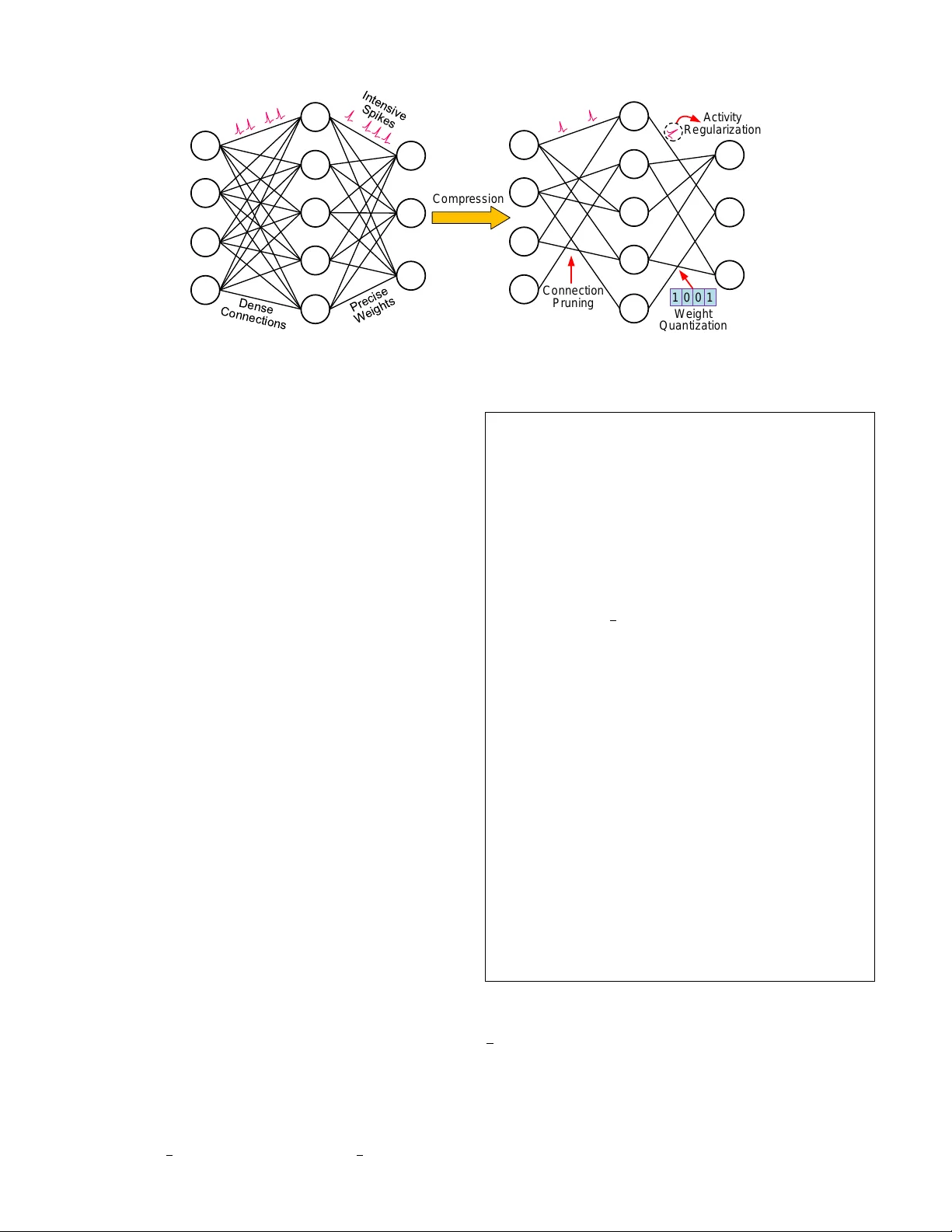
1 Comprehensi v e SNN Compression Using ADMM Optimization and Acti vity Regularization Lei Deng, Member , IEEE , Y ujie W u, Y ifan Hu, Ling Liang, Guoqi Li, Member , IEEE , Xing Hu, Y ufei Ding, Peng Li, F ellow , IEEE , Y uan Xie, F ellow , IEEE Abstract —As well known, the huge memory and compute costs of both artiﬁcial neural networks (ANNs) and spiking neural networks (SNNs) greatly hinder their deployment on edge devices with high efﬁciency . Model compression has been pr oposed as a promising technique to impro ve the running efﬁciency via param- eter and operation reduction. Whereas, this technique is mainly practiced in ANNs rather than SNNs. It is interesting to answer how much an SNN model can be compressed without compromis- ing its functionality , wher e two challenges should be addressed: i) the accuracy of SNNs is usually sensitive to model compression, which requires an accurate compression methodology; ii) the computation of SNNs is event-dri ven rather than static, which produces an extra compr ession dimension on dynamic spikes. T o this end, we realize a comprehensiv e SNN compression through three steps. First, we formulate the connection pruning and weight quantization as a constrained optimization problem. Second, we combine spatio-temporal backpropagation (STBP) and alternating dir ection method of multipliers (ADMM) to solve the problem with minimum accuracy loss. Third, we further propose activity regularization to reduce the spike ev ents for fewer active operations. These methods can be applied in either a single way f or moderate compr ession or a joint way f or aggressive compression. W e deﬁne several quantitative metrics to ev aluation the compression performance for SNNs. Our methodology is validated in pattern r ecognition tasks o ver MNIST , N-MNIST , CIF AR10, and CIF AR100 datasets, where extensive comparisons, analyses, and insights are provided. T o our best knowledge, this is the ﬁrst work that studies SNN compression in a comprehensiv e manner by exploiting all compressible components and achieves better results. K eywor ds: SNN Compression, Connection Pruning, W eight Quantization, Activity Regularization, ADMM I . I N T R O D U C T I O N Neural networks, constructed by a plenty of nodes (neu- rons) and connections (synapses), are powerful in information representation, which has been evidenced in a wide spectrum The work was partially supported by National Science Foundation (Grant No. 1725447), Tsinghua University Initiative Scientiﬁc Research Program, Tsinghua-Foshan Innov ation Special Fund (TFISF), and National Natural Science Foundation of China (Grant No. 61876215). Lei Deng and Y ujie W u contributed equally to this work, corresponding authors: Guoqi Li and Xing Hu. Lei Deng is with the Center for Brain Inspired Computing Research, Department of Precision Instrument, Tsinghua Univ ersity , Beijing 100084, China, and also with the Department of Electrical and Computer Engineering, University of California, Santa Barbara, CA 93106, USA (email: leideng@ucsb .edu). Y ujie Wu, Y ifan Hu, and Guoqi Li are with the Center for Brain Inspired Computing Research, Department of Precision Instrument, Tsinghua University , Beijing 100084, China (email: { wu-yj16, huyf19 } @mails.tsinghua.edu.cn, liguoqi@mail.tsinghua.edu.cn). Ling Liang, Peng Li, and Y uan Xie are with the Department of Electrical and Computer Engineering, University of California, Santa Barbara, CA 93106, USA (email: { lingliang, lip, yuanxie } @ucsb.edu). Xing Hu is with the State Ke y Labora- tory of Computer Architecture, Institute of Computing T echnology , Chinese Academy of Sciences, Beijing 100190, China (email: huxing@ict.ac.cn). Y ufei Ding is with the Department of Computer Science, University of California, Santa Barbara, CA 93106, USA (email: yufeiding@cs.ucsb.edu). of intelligent tasks such as visual or auditory recognition [1]– [4], language modelling [5], [6], medical diagnosis [7], [8], game playing [9], heuristic solution of hard computational problems [10], sparse coding [11], etc. The models include two categories: application-oriented artiﬁcial neural networks (ANNs) and neuroscience-oriented spiking neural networks (SNNs). The former process continuous signals layer by layer with nonlinear activ ation functions; while the latter integrate temporal information via neuronal dynamics and use binary spike signals (0-nothing or 1-spike ev ent) for inter-neuron communication. The success of these models spurs numerous researchers to study domain-speciﬁc hardwares for ANNs and SNNs, termed as deep learning accelerators [12]–[14] and neuromorphic chips [15]–[17], respectively . Whereas, the huge amount of parameters and operations in neural networks greatly limits the running performance and hinders the deployment on edge de vices with tight re- sources. T o solve this problem, various model compression technologies including low-rank decomposition [18], network sparsiﬁcation [19]–[22], and data quantization [23]–[26] have been proposed to shrink the model size, which is quite helpful in boosting the hardware performance [27]–[33]. Although this solution has become a promising way to reduce the memory and compute costs in deep learning, it has yet to be well stud- ied in the neuromorphic computing domain. The underlying reason is because the behaviors of SNNs are quite dif ferent from those of ANNs. For example, i) the spike coding of SNNs makes the accurac y very sensiti ve to model compression , which demands an accurate compression methodology; ii) the processing of SNNs is event-dri ven with a dynamic rather than static execution pattern, which produces an extra compression dimension on dynamic spikes. In fact, we ﬁnd sev eral previous work that tried tentati ve explorations on the SNN compression topic. A two-stage growing-pruning algorithm for compact fully-connected (FC) SNNs was veriﬁed on small-scale datasets [34]. Based on a single FC layer with spike timing dependent plasticity (STDP) learning rule, a soft-pruning method (setting part of weights to a lower bound during training) achie ved 95.04% accuracy on MNIST [35]. Similarly on FC-based SNNs with STDP , both connection pruning and weight quantization were conducted and validated on MNIST with 91.5% accuracy [36]. Combining an FC feature extraction layer with binary weights trained by stochastic STDP and an FC classiﬁcation layer with 24-bit precision, A. Y ousefzadeh et al. [37] presented 95.7% accuracy on MNIST . S. K. Esser et al. [3] adapted normal ANN models to their variants with ternary weights and binary activ ations, and then deployed them on the T rueNorth chip that only supports SNNs. B. Rueckauer et al. [38] conv erted 2 the binarized ANN models to their SNN counterparts and then analyzed the accuracy-vs.-operations trade-off. Howe ver , the techniques with adaption from ANNs suf fers from costly computation in the ANN domain and con version between ANN and SNN, ev en though we only expect the resulting compressed SNN model. G. Srini vasan et al. [39] introduced residual paths into SNNs and combined spiking conv olutional (Con v) layers with binary weight kernels trained by probabilis- tic STDP and non-spiking FC layers trained by conv entional backpropagation (BP) algorithm, which demonstrated 98.54% accuracy on MNIST but only 66.23% accuracy on CIF AR10. Unfortunately , these existing w orks on SNN compression did not either harness large-scale models with impressive performance or touch normal SNNs (just ANN variants, not straightfow ard enough for the SNN compression ). Hence, we formally raise a question that how much an SNN model can be compr essed without compr omising much functionality . W e answer this question through three steps. (1) First, we formulate the connection pruning and the weight quantization as a constrained optimization problem based on supervised learning. (2) Second, we combine the emerging spatio-temporal backpropagation (STBP) supervised learning [40], [41] and the powerful alternating direction method of multipliers (ADMM) optimization tool [42] to solve the problem with minimum accuracy loss. (3) Third, we propose activity regularization to reduce the number of spik e e vents, leading to fe wer active operations. These approaches can be ﬂexibly used in a single or joint manner according to ac- tual needs for compression performance. W e comprehensively validate our methods in SNN-based pattern recognition tasks ov er MNIST , N-MNIST , CIF AR10, and CIF AR100 datasets. Sev eral quantitative metrics to ev aluate the compression ratio are deﬁned, based on which a variety of comparisons between different compression strategies and in-depth result analyses are conducted. Our work can achiev e aggressive compression ratio with adv anced accuracy maintaining, which promises ultra-efﬁcient neuromorphic systems. For better readability , we brieﬂy summarize our contrib u- tions as follows: • W e present the ﬁrst work that in vestigates comprehensiv e and aggressi ve compression for SNNs by exploiting all compressible components and deﬁning quantitati ve ev al- uation metrics. • The ef fectiveness of the ADMM optimization tool is validated on SNNs to reduce the parameter memory space and baseline compute cost for the ﬁrst time. Then, the activity regularization method is further proposed to reduce the number of active operations. All the proposed approaches can be ﬂexibly applied in either a single way for moderate compression or a joint way for aggressi ve compression. • W e demonstrate high compression performance in SNN- based pattern recognition tasks with acceptable accuracy degradation. Rich contrast experiments, in-depth result analyses, and interesting insights are provided. The rest of this paper is organized as follows: Section II introduces some preliminaries of the SNN model, the STBP learning algorithm, and the ADMM optimization approach; Section III systematically explains the possible compression ways, the proposed ADMM-based connection pruning and weight quantization, the activity regularization, their joint use, and the e v aluation metrics; The experimental setup, experi- mental results, and in-depth analyses are provided in Section IV; Finally , Section V concludes and discusses the paper . I I . P R E L I M I N A R I E S A. Spiking Neural Networks In a neural network, neurons behave as the basic processing units which are wired by abundant synapses. Each synapse has a weight that affects the signal transfer efﬁcac y . Figure 1 presents a typical spiking neuron, which is comprised of synapses, dendrites, soma, and axon. Dendrites integrate the weighted input spikes and the soma consequently conducts nonlinear transformation to produce output spikes, then the axon transfers these output spikes to post-neurons. The neu- ronal behaviors can be described by the classic leak y integrate- and-ﬁre (LIF) model [43] as follows:      τ du ( t ) dt = − [ u ( t ) − u r 1 ] + P j w j P t k j ∈ [ t − T w , t ] K ( t − t k j ) ( o ( t ) = 1 & u ( t ) = u r 2 , if u ( t ) ≥ u th o ( t ) = 0 , if u ( t ) < u th (1) where ( t ) denotes the timestep, τ is a time constant, u is the membrane potential of current neuron, and o is the output spike ev ent. w j is the synaptic weight from the j -th input neuron to the current neuron, and t k j is the timestep when the k -th spike from the j -th input neuron comes during the past integration time window of T w . K ( · ) is a kernel function describing the temporal decay effect that a more recent spike should have a greater impact on the post-synaptic membrane potential. u r 1 and u r 2 are the resting potential and reset potential, respectiv ely , and u th is a threshold that determines whether to ﬁre a spike or not. o 0 ∑ So ma S y n a p s e w 1 i n p u t s p i k e s s p i k e s 1 1 1 0 o 1 0 1 1 u th u A x o n Figure 1. Illustration of a spiking neuron comprised of synapses, dendrites, soma, and axon. According to Equation (1), SNNs have the following dif- ferences compared with ANNs: (1) each neuron has temporal dynamics, i.e. memorization of the historical states; (2) the multiplication operations during integration can be removed when T w = 1 o wing to the binary spike inputs; (3) the network acti vities are very sparse because each neuron remains silent if the membrane potential does not exceed the ﬁring threshold. In summary , the temporal memorization makes it well-suited for dynamic d ata with timing information, and the 3 spike-dri ven paradigm with sparse activities enables po wer- efﬁcient asynchronous circuit design. B. STBP Supervised Learning There exist three categories of learning algorithms for SNNs: unsupervised [44], [45], indirectly supervised [46]– [48], and directly supervised [40], [41], [49], [50]. Note that here the “indirectly supervised” mainly refers to the ANN-to- SNN-con version learning. It adopts supervised learning during training, whereas, the supervised learning is applied on the ANN model rather than the SNN one conv erted from the ANN during inference. In contrast, the supervised learning is directly applied on the SNN model in “directly supervised” algorithms. Since SNN compression requires an accurate learning method and the ADMM optimization (to be shown latter) relies on the supervised learning framew ork, we select an emerging directly supervised training algorithm, named spatio-temporal back- propagation (STBP) [40], [41]. W e do not use the indirectly supervised training due to the complex model transformation between ANNs and SNNs. STBP is based on an iterativ e version of the LIF model in Equation (1). Speciﬁcally , it yields ( u t +1 ,n +1 i = e − dt τ u t,n +1 i (1 − o t,n +1 i ) + P j w n ij o t +1 ,n j o t +1 ,n +1 i = H ( u t +1 ,n +1 i − u th ) (2) where dt is the length of the simulation timestep, o denotes the neuronal spike output, t and n are indices of timestep and layer, respectively . e − dt τ reﬂects the leakage effect of the membrane potential. H ( · ) is the Heaviside step function, i.e., H ( x ) = 1 when x ≥ 0 ; H ( x ) = 0 otherwise. This iterative LIF format incorporates all behaviors including integration, ﬁre, and reset in the original neuron model. For simplicity , here we set the parameters in Equation (1) with u r 1 = u r 2 = 0 , T w = 1 , and K ( · ) ≡ 1 . STBP uses rate coding to represent information, wherein the number of spikes matters. The loss function is given by L = k Y Y Y label − 1 T T X t =1 O O O t,N k 2 2 . (3) This loss function measures the discrepanc y between the ground truth and the ﬁring rate of the output layer (i.e. the N -th layer) during the gi ven simulation time window T . In fact, Equation (3) reﬂects ho w to determine the recognition accuracy: i) each output neuron integrates the spikes along all the T timesteps and normalizes the result by dividing T to get a normalized average ﬁre rate value within [0 , 1] ; ii) the output neuron with the largest average ﬁre rate corresponds to the recognized class. Giv en Equation (2)-(3), the gradient propagation and pa- rameter update in STBP can be deriv ed as follows          ∂ L ∂ o t,n i = P j ∂ L ∂ u t,n +1 j ∂ u t,n +1 j ∂ o t,n i + ∂ L ∂ u t +1 ,n i ∂ u t +1 ,n i ∂ o t,n i , ∂ L ∂ u t,n i = ∂ L ∂ o t,n i ∂ o t,n i ∂ u t,n i + ∂ L ∂ u t +1 ,n i ∂ u t +1 ,n i ∂ u t,n i , 5 w n j i = P T t =1 ∂ L ∂ u t,n +1 j o t,n i . (4) The deriv ative approximation method can be used to calcu- late ∂ o ∂ u [40]. Speciﬁcally , it is governed by ∂ o ∂ u = H 0 ≈ boxcar ( u th − a 2 , u th + a 2 ; u ) . Note that boxcar ( u th − a 2 , u th + a 2 ; u ) is the boxcar function deﬁned by the sum of two Heavi- side step functions, i.e., 1 a { H [ u − ( u th − a 2 )] − H [ u − ( u th + a 2 )] } , where a is a hyper-parameter that determines the gradient width. C. ADMM Optimization T ool ADMM is a classic and powerful tool to solve constrained optimization problems [42]. The main idea of ADMM is to decompose the original non-differentiable optimization prob- lem to a dif ferentiable sub-problem which can be solved by gradient descent and a non-differentiable sub-problem with an analytical or heuristic solution. The basic problem of ADMM can be described as min X X X , Z Z Z f ( X X X ) + g ( Z Z Z ) , s.t. A X X X + BZ Z Z = C C C (5) where we assume X X X ∈ R N , Z Z Z ∈ R M , A ∈ R K × N , B ∈ R K × M , C C C ∈ R K . f ( · ) is the major cost function which is usually differentiable and g ( · ) is an indicator of constraints which is usually non-differentiable. Then, the greedy opti- mization of its augmented Lagrangian [42], L ρ ( X X X , Z Z Z , Y Y Y ) = f ( X X X ) + g ( Z Z Z ) + Y Y Y T ( A X X X + BZ Z Z − C C C ) + ρ 2 k A X X X + BZ Z Z − C C C k 2 2 , can be iteratively calculated by          X X X n +1 = arg min X X X L ρ ( X X X , Z Z Z n , Y Y Y n ) Z Z Z n +1 = arg min Z Z Z L ρ ( X X X n +1 , Z Z Z , Y Y Y n ) Y Y Y n +1 = Y Y Y n + ρ ( A X X X n +1 + BZ Z Z n +1 − C C C ) (6) where Y Y Y is the Lagrangian multipliers and ρ is a penalty coef- ﬁcient. The X X X minimization sub-problem is differentiable that is easy to solve via gradient descent. The Z Z Z minimization sub- problem is non-differentiable, but fortunately it can usually be solved analytically or heuristically . I I I . S P I K I N G N E U R A L N E T W O R K C O M P R E S S I O N In this section, we ﬁrst give the possible compression ways, and then explain the proposed compression approaches, algorithms, and ev aluation metrics in detail. A. P ossible Compr ession W ays The compression of SNNs in this work targets the reduction of memory and computation in inference. Figure 2 illustrates the possible ways to compress an SNN model. On the memory side, synapses occupy the most storage space. There are usu- ally two ways to reduce the synapse memory: the number of connections and the bitwidth of weights. On the compute side, although the connection pruning and the weight quantization already help reduce the amount of operations, there is an additional compression way on the dynamic spikes. As well known, the total number of operations for an SNN layer can be gov erned by N ops · R [51], where N ops is the number of baseline operations and R ∈ [0 , 1] is the av erage spike rate per neuron per timestep that usually determines the acti ve power of neuromorphic chips [16]. 4 C o n n e ct i o n Pru n i n g 1 0 0 1 W e i g h t Q u a n t i za t i o n Act i vi t y R e g u l a ri za t i o n C o mp re ssi o n Figure 2. Possible ways for SNN inference compression: connection pruning and weight quantization for memory saving and baseline operation reduction, and activity regularization for activ e operation reduction. T o realize a comprehensi ve SNN compression consider- ing all the above ways, we ﬁrst try to combine the STBP supervised learning and the ADMM optimization tool for connection pruning and weight quantization to shrink memory and reduce N ops . The reason that we combine STBP and ADMM is two-fold: (1) ADMM recently shows an impressiv e compression ratio with good accuracy maintaining in the ANN domain [22], [52]–[55]; (2) ADMM requires a supervised learning framew ork, which excludes the con ventional unsu- pervised learning algorithms for SNNs. Then, besides synapse compression, we additionally propose an activity re gulariza- tion to reduce R for a further reduction of operations. W e will explain these methods one by one in the rest subsections. B. ADMM-based Connection Pruning For the connection pruning, the ADMM problem in Equa- tion (5) can be re-formulated as min W W W ∈ P L = f ( W W W ) (7) where L is the normal STBP loss function in Equation (3) and P denotes a sparse connection space. T o match the indicator item in Equation (5), two steps are required. First, an e xtra indicator function g ( W W W ) is added as follows min W W W f ( W W W ) + g ( W W W ) , (8) where g ( W W W ) = 0 if W W W ∈ P , g ( W W W ) = + ∞ otherwise. Second, it is further conv erted to min W W W , Z Z Z L = f ( W W W ) + g ( Z Z Z ) , s.t. W W W = Z Z Z . (9) Now the pruning problem is equiv alent to the classic ADMM problem gi ven in Equation (5). W ith the constraint of W W W = Z Z Z , the augmented Lagrangian can be equi valently simpliﬁed to L ρ = f ( W W W ) + g ( Z Z Z ) + Y Y Y T ( W W W − Z Z Z ) + ρ 2 k W W W − Z Z Z k 2 2 = f ( W W W ) + g ( Z Z Z ) + ρ 2 k W W W − Z Z Z + e Y Y Y k 2 2 − Data: s (connection sparsity) Step I: ADMM Retraining for Pruning Initialize W W W 0 with the pre-trained weights; Initialize e Y Y Y 0 = 0 0 0 ; Initialize Z Z Z 0 p with W W W 0 and zero out the s % magnitude-smallest elements; Data: W W W n , Z Z Z n p , and e Y Y Y n after the n -th iteration Result: W W W n +1 , Z Z Z n +1 p , and e Y Y Y n +1 1. Re write the loss function: L ⇐ f ( W W W ) + ρ 2 k W W W − Z Z Z n p + e Y Y Y n k 2 2 ; 2. Update weights: W W W n +1 ⇐ retrain the SNN model one more iteration; 3. Update Z Z Z n +1 p : Z Z Z n +1 p ⇐ [zero out the s fraction of magnitude-smallest elements in ( W W W n +1 + e Y Y Y n ) ]; 4. Update e Y Y Y n +1 : e Y Y Y n +1 ⇐ ( e Y Y Y n + W W W n +1 − Z Z Z n +1 p ) ; Step II: Hard-Pruning Retraining Initialize W W W 0 p with the weights from Step I; Initialize the loss function L = f ( W W W p ) ; Data: W W W n p after the n -th iteration Result: W W W n +1 p Update weights: W W W n +1 p ⇐ retrain the SNN model one more iteration; W W W n +1 p ⇐ [zero out the s fraction of magnitude-smallest elements in W W W n +1 p ]; Algorithm 1: ADMM-based Connection Pruning ρ 2 k e Y Y Y k 2 2 where e Y Y Y = Y Y Y /ρ . In this way , the greedy minimization in Equation (6) can be re-written as          W W W n +1 = arg min W W W L ρ ( W W W , Z Z Z n , e Y Y Y n ) Z Z Z n +1 = arg min Z Z Z L ρ ( W W W n +1 , Z Z Z , e Y Y Y n ) e Y Y Y n +1 = e Y Y Y n + W W W n +1 − Z Z Z n +1 . (10) 5 Actually , the ﬁrst sub-problem is W W W n +1 = arg min W W W f ( W W W ) + ρ 2 k W W W − Z Z Z n + e Y Y Y n k 2 2 which is differentiable and can be directly solved by gradient descent. The second sub-problem is Z Z Z n +1 = arg min Z Z Z g ( Z Z Z ) + ρ 2 k W W W n +1 − Z Z Z + e Y Y Y n k 2 2 , which is equiv alent to arg min Z Z Z ∈ P ρ 2 k W W W n +1 − Z Z Z + e Y Y Y n k 2 2 . (11) The abov e sub-problem can be heuristically solved by keeping a fraction of elements in ( W W W n +1 + e Y Y Y n ) with the lar gest magnitudes and setting the rest to zero [22], [53]–[55]. Given W W W n +1 and Z Z Z n +1 , e Y Y Y can be updated according to e Y Y Y n +1 = e Y Y Y n + W W W n +1 − Z Z Z n +1 . The ov erall training for ADMM-based connection pruning is provided in Algorithm 1. Note that the sparsiﬁcation step when updating Z Z Z is layer-wise rather than network-wise. Data: b (weight bitwidth), I (#quantization iterations) Step I: ADMM Retraining for Quantization Initialize W W W 0 with the pre-trained weights; Initialize e Y Y Y 0 = 0 0 0 ; Initialize Z Z Z 0 q = Quan ( W W W 0 , b, I ) ; Data: W W W n , Z Z Z n q , and e Y Y Y n after the n -th iteration Result: W W W n +1 , Z Z Z n +1 q , and e Y Y Y n +1 1. Re write the loss function: L ⇐ f ( W W W ) + ρ 2 k W W W − Z Z Z n q + e Y Y Y n k 2 2 ; 2. Update weights: W W W n +1 ⇐ retrain the SNN model one more iteration; 3. Update Z Z Z n +1 q : Z Z Z n +1 q ⇐ Quan ( W W W n +1 + e Y Y Y n , b, I ) ; 4. Update e Y Y Y n +1 : e Y Y Y n +1 ⇐ ( e Y Y Y n + W W W n +1 − Z Z Z n +1 q ) ; Step II: Hard-Quantization Retraining Initialize W W W 0 q with the weights from Step I; Initialize the loss function L = f ( W W W q ) ; Data: W W W n q after the n -th iteration Result: W W W n +1 q Update weights: W W W n +1 q ⇐ retrain the SNN model one more iteration; W W W n +1 q ⇐ Quan ( W W W n +1 q , b, I ) ; Algorithm 2: ADMM-based W eight Quantization C. ADMM-based W eight Quantization The overall framework of ADMM-based weight quantiza- tion is very similar to the ADMM-based connection pruning. The only dif ference is that the constraint on weights changes from the sparse one to a quantized one. Hence, Equation (7) can be re-written as min W W W ∈ Q L = f ( W W W ) . (12) Q is a set of discrete levels, e.g. Q = α { 0 , ± 2 0 , ± 2 1 , ..., ± 2 b − 1 } , where b is the bitwidth and α is a scaling factor that can be independent between layers. Notice that giv en the bitwidth b , there are 2 b + 1 discrete lev els with our deﬁnition. In the cases of b ≤ 2 , we need b + 1 bits to store the 2 b + 1 lev els; while in the cases of b > 2 , we only need b bits or ev en fewer . For simplicity , we generally denote the needed number of bits as b . Although we follow the deﬁnition of Q in [52], our approach still works under other deﬁnitions. Similarly , now Equation (11) should be arg min Z Z Z ∈ Q ρ 2 k W W W n +1 − Z Z Z + e Y Y Y n k 2 2 , (13) which is equiv alent to arg min e Z Z Z ,α ρ 2 k V V V − α e Z Z Z k 2 2 (14) where V V V = W W W n +1 + e Y Y Y n , α e Z Z Z = Z Z Z , and e Z Z Z ⊂ { 0 , ± 2 0 , ± 2 1 , ..., ± 2 b − 1 } . This sub-problem can also be heuristically solved by an iterative quantization [52], i.e. iteratively ﬁxing α and the quantized vector e Z Z Z to conv ert the biv ariate optimiza- tion to two iterative uni variate optimizations. Speciﬁcally , with α ﬁxed, the quantized vector e Z Z Z is actually the projection of V V V α onto { 0 , ± 2 0 , ± 2 1 , ..., ± 2 b − 1 } , which can be simply obtained by approaching the closest discrete lev el of each element; with e Z Z Z ﬁxed, α can be easily calculated by α = V V V T e Z Z Z e Z Z Z T e Z Z Z . In practice, we ﬁnd this iterativ e minimization conv erges very fast (e.g. in three iterations). The overall training for ADMM- based weight quantization is given in Algorithm 2, where the quantization function ( Quan ( · ) ) is additionally giv en in Algorithm 3. Note that the quantization step when updating Z Z Z is layer-wise too, which might cause different α values across layers. Data: V V V , b (weight bitwidth), I (#quantization iterations) Result: Z Z Z Deﬁne a discrete space Q = { 0 , ± 2 0 , ± 2 1 , ..., ± 2 b − 1 } ; Initialize α = 1 ; for i = 0 : I − 1 do 1. Update e Z Z Z : e Z Z Z ⇐ project each element in V V V α to its nearest discrete le vel in Q ; 2. Update α : α ⇐ V V V T e Z Z Z e Z Z Z T e Z Z Z ; end Z Z Z ⇐ α e Z Z Z ; Algorithm 3: Quantization Function - Quan ( · ) Figure 3 presents the e volution of the weight space during ADMM retraining. In fact, Z Z Z strictly satisﬁes the constraints (sparse or quantized) at each iteration by solving Equation (11) or (13), respectiv ely . Moreover , W W W gradually approaches Z Z Z by minimizing the L 2 -norm regularizer , i.e. ρ 2 k W W W − Z Z Z n + e Y Y Y n k 2 2 , in the ﬁrst sub-problem of ADMM. The auxiliary variable e Y Y Y tends to be zero (we omit it in Figure 3 for simplicity). T o 6 W 0 W 1 W 2 … Z 0 Z 1 Z 2 … C o n s t ra i n i n g C o n s t ra i n i n g C o n s t ra i n i n g F r e e S p a ce Co n st r a in e d S p a ce Figure 3. W eight space e volution during ADMM training. At each iteration, Z Z Z is obtained by constraining W W W into a constrained space and W W W gradually approaches Z Z Z . evidence the above prediction, we visualize the distributions of W W W , Z Z Z , and e Y Y Y at different stages during the entire ADMM retraining process, as depicted in Figure 4. Here we take the weight quantization as an example and set ρ = 0 . 1 . Appar- ently , Z Z Z is always in a quantized space with limited lev els while W W W gradually approaches Z Z Z as ADMM retraining goes on. Notice that although the distributions of Z Z Z seem similar and unchanged due to the limited weight lev els, its value at each element indeed changes until con vergence. Compared to the hard pruning [19], [56] or quantization [25], [57], ADMM- based compression is able to achiev e better conv ergence due to the multiv ariable optimization. Figure 4. Ev olution of W W W , Z Z Z , e Y Y Y during ADMM retraining. D. Activity Regularization As aforementioned in Section III-A, the compute cost of SNNs is jointly determined by the baseline operations and the av erage spike rate during runtime. Hence, besides the connection pruning and the weight quantization, there is an extra opportunity to reduce the compute cost by activity regularization. T o this end, we tune the loss function to L = L normal + λR (15) where L normal is the vanilla loss function in Equation (3), R is the mentioned average spike rate per neuron per timestep, and λ is a penalty coefﬁcient. The reason that we use the av erage spike rate rather than the total number of spikes is to unify the exploration of λ setting across dif ferent networks. By introducing the abov e regularization item, we can further sparsify the ﬁring activities of an SNN model, resulting in decreased acti ve operations. In essence, a similar but dif ferent work was pioneered in [58]. It adopted the mentioned ANN-to-SNN-con version learning method that is distinct from our direct training of SNNs. The activity regularization in [58] was applied on the activ ations of the ANN model during training, indirectly lowering the number of spikes in the resulting SNN model con verted from the ANN model during inference. The ef- fectiv eness of the approach is based on an expectation that the neuronal activ ation of an ANN neuron is proportional to the spike rate of its con verted SNN neuron. By contrast, our activity regularization is directly applied on the spikes of neurons in the SNN model, which does not rely on such an assumption. E. Compr ession Strate gy: Single-way or Joint-way Based on the ADMM-based connection pruning and weight quantization, as well as the activity regularization, we propose two categories of compression strategy: single-way and joint- way . Speciﬁcally , i) single-way compression individually applies connection pruning, weight quantization, or activity regularization; ii) joint-way compression jointly applies con- nection pruning, weight quantization, and activity regulariza- tion, including “Pruning & Regularization”, “Quantization & Regularization”, “Pruning & Quantization”, and “Pruning & Quantization & Regularization”. Compared to the single-way compression, the joint-way compression can usually achie ve a more aggressive ov erall compression ratio by exploiting multiple information ways. For “Pruning & Regularization” and “Quantization & Reg- ularization”, we introduce the acti vity regularization item λR into the loss functions in Algorithm 1 and Algorithm 2, respectiv ely . For “Pruning & Quantization”, we merge both the connection pruning and the weight quantization, as presented in Algorithm 4. F or “Pruning & Quantization & Regulariza- tion”, we further incorporate the acti vity regularization item into the loss function in Algorithm 4. F . Quantitative Evaluation Metrics for SNN Compr ession The compression ratio can be reﬂected by the reduced mem- ory and compute costs. On the memory side, we just count the required storage space for weight parameters since they occupy the most memory space. On the compute side, we just count the required addition operations because multiplications can be remov ed from SNNs with binary spike representation. The connection pruning reduces the number of parameters and baseline operations, thus lowering both the memory and compute costs; the weight quantization reduces the bitwidth of parameters and the basic cost of each addition operation, thus also lo wering both the memory and compute costs; the activity regularization reduces the number of dynamic spikes, thus mainly lo wering the compute cost. Note that although 7 Data: s (connection sparsity), b (weight bitwidth), I (#quantization iterations) Step I: ADMM Retraining for Pruning Initialize W W W 0 with the pre-trained weights; Generate sparse weights W W W p by retraining the SNN model with Algorithm 1; Generate a binary mask M M M p in which 1s and 0s denote the remained and pruned weights in W W W p , respecti vely; Step II: ADMM Retraining for Pruning & Quantization Initialize W W W 0 with the weights from Step I; Initialize e Y Y Y 0 = 0 0 0 ; Initialize Z Z Z 0 pq = Quan ( W W W 0 , b, I ) ; Data: W W W n , Z Z Z n pq , and e Y Y Y n after the n -th iteration Result: W W W n +1 , Z Z Z n +1 pq , and e Y Y Y n +1 1. Re write the loss function: L ⇐ f ( W W W ) + ρ 2 k W W W − Z Z Z n pq + e Y Y Y n k 2 2 ; 2. Update weights: W W W n +1 ⇐ retrain the SNN model one more iteration (update only the non-zero weights according to M M M p ); 3. Update Z Z Z n +1 pq : Z Z Z n +1 pq ⇐ Quan ( W W W n +1 + e Y Y Y n , b, I ) ; 4. Update e Y Y Y n +1 : e Y Y Y n +1 ⇐ ( e Y Y Y n + W W W n +1 − Z Z Z n +1 pq ) ; Step III: Hard-Pruning-Quantization Retraining Initialize W W W 0 pq with the weights from Step II; Initialize the loss function L = f ( W W W pq ) ; Data: W W W n pq after the n -th iteration Result: W W W n +1 pq Update weights: W W W n +1 pq ⇐ retrain the SNN model one more iteration (update only the non-zero weights according to M M M p ); W W W n +1 pq ⇐ Quan ( W W W n +1 pq , b, I ) ; Algorithm 4: ADMM-based Pruning & Quantization fewer spikes can also reduce the associated memory access, the memory trafﬁc cost depends on actual hardware architectures, which is out the scope of this algorithm-level paper . Therefore, we only discuss the reduction of the compute cost when applying acti vity regularization. Here we propose several metrics to quantitativ ely ev aluate the compression ratio of SNNs. For the memory compression, we deﬁne the following percentage of residual memory cost: R mem = (1 − s ) · b/B (16) where s ∈ [0 , 1] is the connection sparsity , B and b are the weight bitwidth of the original model and the compressed model, respectiv ely . Since the operation compression is related to the dynamic spik es, next, we deﬁne the percentage of residual spikes as R s = r /R (17) if we can reduce the a verage spike rate from R to r . Based on the mentioned rule in Section III-A that the total number of operations in an SNN model is calculated by multiplying the number of baseline operations and the average spike rate, we deﬁne the percentage of residual operation cost as R ops ≈ (1 − s ) · b B · r R = R mem · R s . (18) Note that above equation is just a coarse estimation because the impact of bitwidth on the operation cost is not linear . For example, an FP32 (i.e. 32-bit ﬂoating point) dendrite integration is not strictly 4 × costly than an INT8 (i.e. 8-bit integer) one. I V . E X P E R I M E N TA L R E S U L T S A. Experimental Setup W e validate our compression methodology on various datasets, including the static image datasets (e.g. MNIST , CIF AR10, and CIF AR100) and the e vent-dri ve N-MNIST , and then observ e the compression effect on accurac y and summarize the extent to which an SNN model can be compressed with acceptable functionality degradation. For MNIST and N-MNIST , we use the classic LeNet-5 structure; while for CIF AR10 and CIF AR100 , we use a con volution with stride of 2 to replace the pooling operation and then design a 10-layer spiking con volutional neural network (CNN) with the structure of Input-128C3S1-256C3S2-256C3S1-512C3S2- 512C3S1-1024C3S1-2048C3S2-1024FC-512FC-10/100. W e take the Bernoulli sampling to conv ert the raw pixel intensity to a spike train on MNIST ; while on CIF AR10 and CIF AR100 , inspired by [41], we use an encoding layer to con vert the normalized image input into spike trains to improv e the baseline accuracy . The number of presented timesteps (i.e., the number of dt ) for each input sample is T , which is also the time window for the calculation of the av erage spike rate. The simulation time interv al between consecutive sample presentations is assumed to be long enough to let the membrane potential leak sufﬁciently , av oiding the possible cross-sample interference. The programming en vironment for our experiments is Pytorch. W e omit “INT” and only remain the bitwdith for simplicity in the results with weight quantizaiton. T able I H Y P E R - PA R A M E T E R S E T T I N G O N D I FF E R E N T D A TA S E T S . Parameters Descriptions MNIST N-MNIST CIF AR10 CIF AR100 dt Duration of Simulation Timetep 1 ms 1 ms 1 ms 1 ms N 0 Epochs for Model Pretraining 150 150 100 100 Batch Size – 50 50 50 T Number of Presented Timesteps 10 10 8 8 for Each Sample u th Firing Threshold 0.2 0.4 0.5 0.5 e − dt τ Membrane Potential Decay Factor 0.25 0.3 0.25 0.8 a Gradient Width of H ( · ) 0.5 0.5 0.5 0.5 ρ Penalty Coefﬁcient for ADMM 5e-4 5e-4 5e-4 1e-4 N 1 Retraining Epochs for 10 10 20 20 ADMM-Compression N 2 Retraining Epochs for 10 10 15 20 Hard-Compression(HC) First, connection pruning, weight quantization, and acti vity regularization are ev aluated individually for a preliminary 8 effecti veness estimation. Next, the compression is carried out in a joint way with two or three methods, to explore the comprehensiv e effect and the optimal combination. W e do not compress the ﬁrst and last layers due to their accuracy sensitivity and the insigniﬁcant amount of parameters and operations, so the calculation of R mem and R ops does not include these two layers. Details about the hyper -parameter setting can be seen in T able I. B. Single-way Compression In this subsection, we analyze the results from single-way compression, i.e. applying connection pruning (Figure 5 & T able II), weight quantization (Figure 6 & T able III), and activity regularization (Figure 7 & T able IV) individually . Finally , we present Figure 8 to summary the accuracy results in T able II-IV for a better glance. Figure 5. Ef fect of connection pruning on LeNet-5, (a) visualization of 800 randomly selected connections, where white pixels denote pruned connections; (b) weight value distribution before and after pruning with 75% sparsity . T able II A C C U R AC Y U N D E R D I FF E R E N T C O N N E C T I O N S PA R S I T Y . Dataset Sparsity ( s ) Acc. (%) Acc. Loss (%) MNIST 0% 99.07 0.00 25% 99.19 0.12 40% 99.08 0.01 50% 99.10 0.03 60% 98.64 -0.43 75% 96.84 -2.23 N-MNIST 0% 98.95 0.00 25% 98.72 -0.23 40% 98.59 -0.36 50% 98.34 -0.61 60% 97.98 -0.91 75% 96.83 -2.12 CIF AR10 0% 89.53 0.00 25% 89.8 0.27 40% 89.75 0.18 50% 89.15 -0.38 60% 88.35 -1.18 75% 87.38 -2.15 Connection Pruning . As shown in Figure 5, the number of disconnected synapses dramatically increases after connection pruning, and the overall percentage of pruned connections grows accordingly as the sparsity becomes higher . More speciﬁcally , T able II shows the model accuracy under different pruning ratio (i.e. connection sparsity). Ov erall, a < 40-50% pruning ratio causes negligible accuracy loss or e ven better accuracy due to the alle viation of ov er-ﬁtting, while an over 60% sparsity would cause obvious accuracy degradation that ev en reaches > 2% at 75% sparsity . The accuracy loss on N- MNIST is more sev ere than that on MNIST , especially in the low-sparsity re gion. This reﬂects the accuracy sensiti vity to the connection pruning on N-MNIST with natural sparse features. The accuracy on CIF AR10 drops faster due to the increasing difﬁculty and model size. Figure 6. W eight distribution of LeNet-5 before and after weight quantization under b = 2 . T able III A C C U R AC Y U N D E R D I FF E R E N T W E I G H T B I T W I D T H . Dataset Bitwidth ( b ) Acc. (%) Acc. Loss (%) MNIST 32 (FP) 99.07 0.00 4 99.10 0.03 3 99.04 -0.03 2 98.93 -0.14 1 98.85 -0.22 N-MNIST 32 (FP) 98.95 0.00 4 98.67 -0.28 3 98.65 -0.30 2 98.58 -0.37 1 98.54 -0.41 CIF AR10 32 (FP) 89.53 0.00 4 89.40 -0.13 3 89.32 -0.21 2 89.23 -0.30 1 89.01 -0.52 W eight Quantization . Figure 6 evidences that the number of weight levels can be signiﬁcantly reduced after applying the weight quantization. Note that the number of discrete lev els in the network is more than 5 at b = 2 due to the different scaling factors (i.e., α ) across layers after quantization. Moreov er , T able III presents the accuracy results under dif ferent weight bitwidth. On all datasets, we observe negligible accuracy loss when b ≥ 4 . The accurac y loss is still very small ( ≤ 0.52%) ev en if under the aggressive compression with b = 1 , which reﬂects the effecti veness of our ADMM-based weight quan- tization. The accuracy loss on MNIST is constantly smaller than others due to the simplicity of this task. Activity Regulaization . Different from the compression of synapses in previous connection pruning and weight quantiza- tion, the activity regularization reduces the number of dynamic 9 Figure 7. Effect of activity regularization on LeNet-5 ( λ = 0 . 01 ), (a) spike trains of six randomly selected neurons, where the lower spike train for each neuron is the one after activity regularization; (b) av erage spike rate distribution without and with activity regularization. Here the average spike rate means the average number of spikes per timestep, and the distribution is across neurons. T able IV A C C U R AC Y U N D E R D I FF E R E N T S P I K E R ATE . Dataset λ A vg. Spike Rate ( r ) Acc. Acc. Loss (%) MNIST 0 0.22 99.07 0.00 0.001 0.19 99.22 0.15 0.01 0.12 99.11 0.04 0.1 0.06 98.54 -0.53 N-MNIST 0 0.18 98.95 0.00 0.001 0.17 98.56 -0.39 0.01 0.13 98.53 -0.42 0.1 0.06 98.23 -0.72 CIF AR10 0 0.11 89.53 0.00 0.001 0.11 89.51 -0.02 0.01 0.08 87.62 -1.91 0.1 0.03 81.01 -8.52 spikes thus decreasing the number of acti ve operations. The total number of spike e vents and the average spike rate can be greatly decreased by using this regularization (see Figure 7). T able IV further lists the accuracy results under dif ferent av erage spike rate, which is realized by adjusting λ . A larger λ leads to a more aggressiv e re gularization, i.e. lower spike rate. From MNIST to N-MNIST and CIF AR10, we observe a gradually weak ened rob ustness to the activity regularization. Also, we ﬁnd that the baseline average spike rate under λ = 0 gradually decreases, which indicates that a higher baseline spike rate would have more space for acti vity re gularization without compromising much accuracy . This is straightforward to understand because a higher baseline spike rate usually has a stronger capability for initial information representation. C. J oint-way Compr ession In this subsection, we analyze the results from joint-way compression, i.e. simultaneously applying two or three meth- ods among connection pruning, weight quantization, and acti v- ity regularization. T able V and VI provide the accuracy results of the two-way compression and the three-way compression, respectiv ely . Based on these two tables, we summarize sev eral interesting observ ations as follo ws. Contribution to R mem and R s . The weight quantization contributes most to the reduction of memory (reﬂected by R mem ) compared to the connection pruning. For example, an aggressiv e 75% connection sparsity (i.e. R mem =25%) just cor- responds to a slight 8-bit weight quantization at the same lev el of memory compression ratio. Note that, as aforementioned, a b -bit weight in this work has 2 b + 1 discrete lev els, which is actually more aggressive quantization than the standard deﬁnition with 2 b lev els when b > 2 . By contrast, the activity regularization contributes most to the reduction of spikes (reﬂected by R s ) because it directly decreases the number of spikes. At last, according to Equation (18), R mem and R s jointly determine the reduction of operations (reﬂected by R ops ). T rade-off between R mem and R s . The compression ratios of synapse memory and dynamic spikes actually behave as a trade-off. A too aggressiv e spike compression baseline (e.g. under λ = 0 . 1 ) will cause a large accuracy loss when R mem slightly decreases; a too aggressi ve memory compression base- line (e.g. R mem < 5%) will also cause a signiﬁcant accuracy loss when R s slightly decreases. It is challenging to aggres- siv ely compress both the synapse memory and dynamic spikes without compromising accuracy . Figure 9 evidences this trade- off by visualizing all the joint-way compression results from T able V and VI on the R mem - R s plane. Notice that the point ( R mem = 0 . 78 , R s = 56 . 25% without activity regularization achiev es lo wer accuracy (93.52%) than its neighboring points with higher R mem values or with the same R mem value but using a slight activity regularization (e.g., λ = 0 . 001 , 97.16% and λ = 0 . 01 , 94.56%). This reﬂects that a slight activity regularization can improv e accurac y , someho w like the dropout technique. Furthermore, since we hav e the R ops metric that takes both R mem and R s into account (see Equation (18)), we further visualize the relationship between R ops and accuracy , which is depicted in Figure 10. Note that the data here are collected from T able II-VI. It can be seen that, from a global angle, accurac y is positiv ely correlated to R ops , i.e. a lo wer R ops is prone to cause a lower accuracy . Ho wev er , the local relationship between R ops and accuracy loses monotonicity to some extent and shows slight variance. The underlying reason is due to the imbalanced inﬂuences on accuracy of different single-way compression methods. Ev en if keeping the R ops values very close, it is possible to get variable accuracy scores by adopting different strategies to combine the single- way compression methods, let alone in the cases of obviously different R ops values in Figure 10. The imbalance is e ven increased by the weight quantization that attracts accuracy tow ards the top-left direction, thus increasing the accuracy variance when we look at all the joint-compression points. Joint-way Compr ession v .s. Single-way Compression . W e recommend to gently compress multi-way information rather than to aggressiv ely compress only single-way information. Speciﬁcally , an aggressiv e compression in one w ay (e.g. ≥ 75% connection sparsity , 1 -bit weight bitwidth, or λ ≥ 0 . 1 acti vity regularization) is easy to cause accuracy collapse. In contrast, a gentle compression in each of the multiple ways is able to pro- duce a better ov erall compression ratio while paying smaller accuracy loss. F or example, the accurac y loss is only 0 . 26 % on MNIST when concurrently applying 25% connection pruning, 1 -bit weight quantization, and λ = 0 . 01 activity regularization. In this case, the overall compression ratio actually reaches as 10 Figure 8. Glance of the accuracy results under single compression. T able V A C C U R AC Y O N M N I S T W H E N J O I N T LY A P P L Y I N G T W O C O M P R E S S I O N M E T H O D S . λ Sparsity ( s ) Bitwidth ( b ) A vg. Spike Rate ( r ) R mem 1 R ops 1 Acc.(%) Acc.Loss (%) 0 0% 32 (FP) 0.32 100.00% (1.00 × ) 100.00% (1.00 × ) 99.07 0.00 0.001 25% 32 (FP) 0.19 75.00% (1.33 × ) 43.14% (2.32 × ) 99.11 0.04 0.001 50% 32 (FP) 0.18 50.00% (2.00 × ) 28.30% (3.53 × ) 98.97 -0.10 0.001 75% 32 (FP) 0.15 25.00% (4.00 × ) 11.74% (8.52 × ) 95.30 -3.77 0.01 25% 32 (FP) 0.12 75.00% (1.33 × ) 27.52% (3.63 × ) 99.22 0.15 0.01 50% 32 (FP) 0.12 50.00% (2.00 × ) 18.19% (5.50 × ) 99.13 0.06 0.01 75% 32 (FP) 0.09 25.00% (4.00 × ) 7.15% (13.99 × ) 95.39 -3.68 0.1 25% 32 (FP) 0.06 75.00% (1.33 × ) 13.52% (7.40 × ) 98.70 -0.37 0.1 50% 32 (FP) 0.06 50.00% (2.00 × ) 8.71% (11.48 × ) 98.89 -0.18 0.1 75% 32 (FP) 0.06 25.00% (4.00 × ) 4.51% (22.17 × ) 95.49 -3.66 0.001 0% 3 0.21 9.38% (10.66 × ) 5.98% (16.72 × ) 98.65 -0.42 0.001 0% 2 0.22 6.25% (16.00 × ) 4.18% (23.92 × ) 98.83 -0.24 0.001 0% 1 0.20 3.13% (31.95 × ) 1.94% (51.55 × ) 98.33 -0.74 0.01 0% 3 0.13 9.38% (10.66 × ) 3.73% (26.81 × ) 98.92 -0.15 0.01 0% 2 0.12 6.25% (16.00 × ) 2.41% (41.49 × ) 98.72 -0.35 0.01 0% 1 0.12 3.13% (31.95 × ) 1.19% (84.03 × ) 98.44 -0.63 0.1 0% 3 0.06 9.38% (10.66 × ) 1.72% (58.14 × ) 98.81 -0.26 0.1 0% 2 0.07 6.25% (16.00 × ) 1.34% (74.63 × ) 96.68 -2.39 0.1 0% 1 0.05 3.13% (31.95 × ) 0.48% (208.33 × ) 82.25 -16.82 0 25% 3 0.29 7.03% (14.22 × ) 6.32% (15.82 × ) 98.59 -0.48 0 25% 2 0.26 4.69% (21.32 × ) 3.76% (26.60 × ) 98.75 -0.32 0 25% 1 0.22 2.34% (42.74 × ) 1.63% (61.35 × ) 98.64 -0.43 0 50% 3 0.29 4.69% (21.32 × ) 4.26% (23.47 × ) 98.27 -0.80 0 50% 2 0.29 3.13% (31.95 × ) 2.81% (35.59 × ) 98.53 -0.54 0 50% 1 0.22 1.56% (64.10 × ) 1.07% (93.46 × ) 96.25 -2.82 0 75% 3 0.25 2.34% (42.74 × ) 1.84% (54.35 × ) 97.13 -1.94 0 75% 2 0.21 1.56% (64.10 × ) 1.02% (98.04 × ) 97.01 -1.96 0 75% 1 0.18 0.78% (128.21 × ) 0.45% (222.22 × ) 93.52 -5.55 Note 1 : The compression ratio in the parentheses is the reciprocal of R mem or R ops . aggressiv e as R mem = 2 . 34 % (i.e. 42.74 × compression) and R ops = 0 . 91 % (i.e. 109.89 × compression). If we expect the same R ops using the single-way compression, the accuracy would drop dramatically . Figure 10 reﬂects this guidance too, where the joint-way compression can reduce more R ops with the same level of accuracy loss. Accuracy T olerance to W eight Quantization . Recalling T able II and III, we observe that SNN models usually present a better accuracy tolerance to the weight quantization than the connection pruning. For example, the accuracy loss at 75% connection sparsity could reach > 2%, while the loss at 1-bit weight quantization is only < 0.55%. W e use Figure 11 to further evidence this speculation. It can be seen that, under the same weight compression ratio, we ﬁnd the “aggressi ve quantization & slight pruning” schemes are able to maintain accuracy better than the “slight quantization & aggressi ve pruning” schemes. Robustness on N-MNIST Dataset . From T able VI, we ﬁnd that SNNs on N-MNIST present more graceful accuracy loss against the joint compression than those on other datasets we used, especially in the cases of aggressive compression. For in- stance, the accuracy loss is only about 2% e ven if an extremely 11 T able VI A C C U R AC Y O N M N I S T , C I FA R 1 0 A N D N - M N I S T W H E N A P P L Y I N G A L L T H R E E C O M P R E S S I O N M E T H O D S . Dataset λ Sparsity ( s ) Bitwidth ( b ) A vg. Spike Rate ( r ) R mem 1 R ops 1 Acc. (%) Acc. Loss (%) MNIST 0 0% 32 (FP) 0.33 100.00% (1.00 × ) 100.00% (1.00 × ) 99.07 0.00 0.001 25% 3 0.19 7.03% (14.22 × ) 4.06% (24.63 × ) 98.97 -0.10 0.001 25% 1 0.19 2.34% (42.74 × ) 1.34% (74.63 × ) 99.04 -0.03 0.001 75% 3 0.16 2.34% (42.74 × ) 1.16% (86.21 × ) 97.25 -1.82 0.001 75% 1 0.17 0.78% (128.21 × ) 0.41% (243.90 × ) 97.16 -1.91 0.01 25% 3 0.12 7.03% (14.22 × ) 2.61% (38.31 × ) 99.11 0.04 0.01 25% 1 0.13 2.34% (42.74 × ) 0.91% (109.89 × ) 98.81 -0.26 0.01 75% 3 0.11 2.34% (42.74 × ) 0.75% (133.33 × ) 94.92 -4.15 0.01 75% 1 0.11 0.78% (128.21 × ) 0.25% (400.00 × ) 94.56 -4.51 0.1 25% 3 0.06 7.03% (14.22 × ) 1.29% (77.52 × ) 98.25 -0.82 0.1 25% 1 0.05 2.34% (42.74 × ) 0.36% (277.78 × ) 88.14 -10.93 0.1 75% 3 0.07 2.34% (42.74 × ) 0.49% (204.08 × ) 94.54 -4.43 0.1 75% 1 0.06 0.78% (128.21 × ) 0.13% (769.23 × ) 74.98 -24.09 CIF AR10 0% 0 32 (FP) 0.110 100.00% (1.00 × ) 100.00% (1.00 × ) 89.53 0.00 0.001 25% 3 0.10 7.03% (14.22 × ) 6.14% (16.29 × ) 87.84 -1.69 0.001 25% 1 0.09 2.34% (42.74 × ) 1.81% (55.25 × ) 87.42 -2.11 0.001 75% 3 0.09 2.34% (42.74 × ) 1.85% (54.05 × ) 87.59 -1.94 0.001 75% 1 0.09 0.78% (128.21 × ) 0.6% (166.67 × ) 86.99 -2.54 0.01 25% 3 0.06 7.03% (14.22 × ) 3.71% (26.95 × ) 87.37 -2.16 0.01 25% 1 0.06 2.34% (42.74 × ) 1.3% (76.92 × ) 84.51 -5.02 0.01 75% 3 0.07 2.34% (42.74 × ) 1.43% (69.93 × ) 87.13 -2.40 0.01 75% 1 0.06 0.78% (128.21 × ) 0.39% (256.41 × ) 86.75 -2.78 0.1 25% 3 0.04 7.03% (14.22 × ) 2.24% (44.64 × ) 82.75 -6.78 0.1 25% 1 0.03 2.34% (42.74 × ) 0.66% (151.52 × ) 77.78 -11.75 0.1 75% 3 0.04 2.34% (42.74 × ) 0.74% (135.14 × ) 80.64 -8.89 0.1 75% 1 0.03 0.78% (128.21 × ) 0.22% (454.55 × ) 74.83 -14.70 N-MNIST 0 0% 32 (FP) 0.19 100.00% (1.00 × ) 100.00% (1.00 × ) 98.95 0.00 0.001 25% 3 0.03 7.03% (14.22 × ) 1.29% (77.52 × ) 98.62 -0.33 0.001 25% 1 0.03 2.34% (42.74 × ) 0.43% (232.56 × ) 98.57 -0.38 0.001 75% 3 0.03 2.34% (42.74 × ) 0.35% (285.71 × ) 96.19 -2.76 0.001 75% 1 0.03 0.78% (128.21 × ) 0.13% (769.23 × ) 96.33 -2.62 0.01 25% 3 0.03 7.03% (14.22 × ) 0.97% (103.09 × ) 98.73 -0.22 0.01 25% 1 0.03 2.34% (42.74 × ) 0.32% (312.50 × ) 98.66 -0.29 0.01 75% 3 0.02 2.34% (42.74 × ) 0.28% (357.14 × ) 97.23 -1.72 0.01 75% 1 0.02 0.78% (128.21 × ) 0.1% (1000.00 × ) 97.19 -1.76 0.1 25% 3 0.01 7.03% (14.22 × ) 0.42% (238.10 × ) 98.43 -0.52 0.1 25% 1 0.01 2.34% (42.74 × ) 0.14% (714.29 × ) 98.37 -0.58 0.1 75% 3 0.01 2.34% (42.74 × ) 0.12% (833.33 × ) 96.74 -2.21 0.1 75% 1 0.01 0.78% (128.21 × ) 0.04% (2500.00 × ) 96.87 -2.08 Note 1 : The compression ratio in the parentheses is the reciprocal of R mem or R ops . aggressiv e compression of R mem = 0 . 78 % (i.e. 128.21 × compression) and R ops = 0 . 04 % (i.e. 2500 × compression) is applied. By contrast, this degree of compression on MNIST will cause > 20% accuracy loss. Recalling our observations in single-way compression, SNNs on N-MNIST are more prone to cause higher accuracy degradation than the ones on MNIST under lo w compression ratios. Considering these together , we expect that the underlying reason lies in the sparse features within these ev ent-dri ven datasets (e.g. N-MNIST), where the information is heavily scattered along the temporal dimension. This temporal scattering of information causes accuracy degradation when the model meets any compression (ev en if the compression is slight) due to the sensiti vity of intrinsic sparse features, while signiﬁcantly reducing the accuracy drop when facing an aggressiv e compression owing to the lower data requirement to represent sparse features. D. Effectiveness of ADMM optimization In this subsection, we verify the effecti veness of ADMM optimization. W e compare the accuracy results between the cases with and without ADMM optimization. Note that the compression without ADMM optimization is named hard compression (HC) here. The results are presented in T able VII that in volves both single-way and joint-way compression. The accuracy scores with ADMM optimization are consistently better than those without ADMM optimization, which evi- dences the effecti veness of our ADMM optimization in SNN compression. E. Comparison with Existing SNN Compr ession T able VIII compares our results with other existing works that touch SNN compression. A fair comparison should take both the compression ratio and recognition accuracy into account. In this sense, our approach is able to achiev e a much higher ov erall compression performance, o wing to the accurate STBP learning and the powerful ADMM optimization. Note two points: (1) the recent ReStoCNet [39] is not a pure SNN model where the FC layers use non-spiking neurons and do not apply any compression technique, which signiﬁcantly 12 Figure 9. Accuracy with dif ferent R mem and R s in the joint-way compression on MNIST . All the data are collected from T able V and VI. Figure 10. Relationship between R ops and accuracy on MNIST . All data are collected from T able II-VI. Abbreviations: P-connection pruning, Q-weight quantization, A-activity regularization, “Joint-T wo”–joint-way compression with two single-way compression methods (i.e., pruning & re gularization, quantization & regularization, and pruning & quantization), “Joint-Three”– joint-way compression with all three single-way compression methods (i.e., pruning & quantization & regularization). T able VII C O M PA R I S O N TO H A R D C O M P R E S S I O N ( H C ) W I T H O U T A D M M O P T I M I Z AT I O N O N C I FA R 1 0 . Sparsity ( s ) Bitwidth ( b ) R mem Acc. of HC (%) Acc. of Ours (%) 50% 32 (FP) 50.00% 88.98 89.15 75% 32 (FP) 25.00% 87.00 87.38 90% 32 (FP) 10.00% 77.90 85.68 0% 3 9.38% 88.98 89.32 0% 2 6.25% 88.78 89.23 0% 1 3.13% 88.63 89.01 75% 3 2.34% 80.30 87.27 90% 3 0.94% 75.47 83.35 75% 1 0.78% 78.85 86.71 Figure 11. Accuracy on MNIST under dif ferent weight compression ratio and strategy . R mem is controlled by connection sparsity ( s ) and weight bitwidth ( b ) according to Equation (16). contributes to accuracy maintaining; (2) the models in [38] are trained using the ANN-to-SNN-con version approach, where the required T is usually much larger than ours. T able VIII C O M PA R I S O N W I T H E X I S T I N G S N N C O M P R E S S I O N WO R K S O N M N I S T, C I F A R 1 0 , O R C I FA R 1 0 0 ( T H E D E FAU L T D A TAS E T I S M N I S T U N L E S S OT H E RW I S E S P E C I FI E D ) . H E R E T H E N U M B E R O F L A Y E R S I N C L U D E S T H E I N P U T L A Y E R . Net. Structure Sparsity ( s ) Bitwidth ( b ) Acc. (%) Spiking DBN [59] 4-layer MLP 0% 4 91.35 Pruning & Quantization [36] 2-layer MLP 1 92% ternary 91.50 Soft-Pruning [35] 3-layer MLP 75% 32 (FP) 94.05 Stochastic-STDP [37] 3-layer MLP 0% binary 2 95.70 NormAD [60] 3-layer CNN 0% 3 97.31 ReStoCNet [39] 5-layer CNN 3 0% binary 4 98.54 ReStoCNet (CIF AR10) [39] 5-layer CNN 3 0% binary 4 66.23 Spiking CNN (CIFAR10) [38] 5 9-layer CNN 0% binary 83.35/87.45 6 Spiking CNN (CIFAR100) [3] N.A. 0% ternary 55.64 This work 5-layer CNN 0% 3 99.04 This work 5-layer CNN 25% 1 98.81 7 This work (CIF AR10) 5-layer CNN 8 50% 1 68.52 This work (CIF AR10) 11-layer CNN 50% 1 87.21 This work (CIF AR100) 11-layer CNN 50% 3 57.83 This work (CIF AR100) 11-layer CNN 25% 1 55.95 Note 1 : There is an extra inhibitory layer without compression. Note 2 : The last layer uses 24-bit weight precision. Note 3 : The FC layers use non-spiking neurons. Note 4 : The weights in FC layers are in full precision. Note 5 : The models are trained using the ANN-to-SNN-conv ersion ap- proach, where the required T is usually much larger than ours. Note 6 : The activ ations of the ANN before conversion are also binarized. Note 7 : Additional spike compression ( λ = 0 . 01 ) is applied. Note 8 : For fair comparison, we use the same network structure as [39] and compress only the Conv layers too. Differently , the neurons in our network are all spiking neurons. F . Comparison with ANN-to-SNN-Con version Methodology In essence, ADMM optimization can be applied in both SNN compression and ANN compression, and it is interesting to compare their compression performance. In this subsection, we use an extra e xperiment to do a simple analysis. W e compare with the ANN-to-SNN-con version methodology on MNIST . As gi ven in T able IX, the direct compression of the SNN model using our methodology with 25% connection sparsity ( s = 25% ) and 3-bit weight bitwidth ( b = 3 ) can achiev e 98.59% accuracy . In contrast, although the compressed 13 ANN can achiev e higher accuracy than our compressed SNN, the resulting con verted SNN will lose accuracy during the model conv ersion if T is not large enough. Usually , in order to maintain accuracy , the v alue of T in the ANN-to-SNN- con version methodology needs to be tens of times larger than our T = 10 . T able IX A C C U R AC Y C O M PAR I S O N B E T W E E N T H E A N N - T O - S N N - C O N V E R S I O N M E T H O D O L O G Y A N D O U R D I R E C T T R A I N I N G M E T H O D O L O G Y O N M N I S T . Compressed SNN ( s = 25% , b = 3 , T = 10 ): 98.59% Compressed ANN ( s = 25% , b = 3 ): 98.84% #timestep ( T ) 10 50 100 250 500 1000 Con verted SNN 11.35% 48.51% 80.14% 98.25% 98.75% 98.79% V . C O N C L U S I O N A N D D I S C U S S I O N In this paper, we combine STBP and ADMM to compress SNN models in two aspects: connection pruning and weight quantization, which greatly shrinks the memory space and baseline operations. Furthermore, we propose activity regular - ization to lower the number of dynamic spikes, which reduces the activ e operations. The three compression approaches can be used in a single paradigm or a joint paradigm according to actual needs. Our solution is the ﬁrst work that inv estigates the SNN compression problem in a comprehensiv e manner by ex- ploiting all compressible components and deﬁning quantitativ e ev aluation metrics. W e demonstrate much better compression performance than prior work. Through extensi ve contrast experiments along with in-depth analyses, we observ e sev eral interesting insights for SNN com- pression. First, the weight quantization contributes most to the memory reduction (i.e. R mem ) while the activity regularization contributes most to the spike reduction (i.e. R s ). Second, there is a trade-off between R mem and R s , and R ops representing the overall compression ratio could approximately reﬂect the accuracy after compression. Third, the gentle compression of multi-way information usually pays less accurac y loss than the aggressi ve compression of only single-way information. Therefore, we recommend the joint-way compression if we expect a better overall compression performance. Fourth, we observe that SNN models show a good tolerance to the weight quantization. Finally , the accuracy drop of SNNs on ev ent- driv en datasets (e.g. N-MNIST) is higher than that on static image datasets (e.g. MNIST) under low compression ratios but quite graceful when coming to aggressiv e compression. These observations will be important to determine the best compression strategy in real-world applications with SNNs. Although we provide a powerful solution for comprehensi ve SNN compression, there are still se veral issues that deserv e in vestigations in future work. W e focus more on presenting our methodology and just give limited testing results due to the tight b udgets on page and time. This is acceptable for a starting work to study comprehensi ve SNN compression; whereas, in order to thoroughly understand the joint-way compression and mine more insights, a wider range of experiments (e.g. with different settings of compression hyper -parameters, on different benchmarking datasets, using more intuiti ve visual- izations, etc.) are highly demanded. Reinforcement learning might be a promising tool to search the optimal compression strategy [21], [26] if substantial resources are available. For simplicity , we just focus on the element-wise sparsity with an irregular pattern that impedes efﬁcient running due to the large indexing ov erhead. The structured sparsity [53] seems helpful to optimize the execution performance. Incorporating the hard- ware architecture constraints into the design of compression algorithm should be considered to achiev e practical saving of latency and energy on neuromorphic devices. In addition, the comparison of the compression effects on ANNs and SNNs is also an interesting topic. R E F E R E N C E S [1] K. He, X. Zhang, S. Ren, and J. Sun, “Deep residual learning for image recognition, ” in Pr oceedings of the IEEE confer ence on computer vision and pattern recognition , 2016, pp. 770–778. [2] O. Abdel-Hamid, A.-r . Mohamed, H. Jiang, L. Deng, G. Penn, and D. Y u, “Con volutional neural networks for speech recognition, ” IEEE/ACM T ransactions on audio, speech, and language pr ocessing , vol. 22, no. 10, pp. 1533–1545, 2014. [3] S. K. Esser, P . A. Merolla, J. V . Arthur , A. S. Cassidy , R. Appuswamy , A. Andreopoulos, D. J. Ber g, J. L. McKinstry , T . Melano, D. R. Barch, C. di Nolfo, P . Datta, A. Amir, B. T aba, M. D. Flickner, and D. S. Modha, “Conv olutional networks for fast, energy-efﬁcient neuromorphic computing, ” Proceedings of the National Academy of Sciences , vol. 113, no. 41, pp. 11 441–11 446, 2016. [4] P . U. Diehl, B. U. Pedroni, A. Cassidy , P . Merolla, E. Neftci, and G. Zarrella, “T ruehappiness: Neuromorphic emotion recognition on truenorth, ” in Neural Networks (IJCNN), 2016 International Joint Con- fer ence on . IEEE, 2016, pp. 4278–4285. [5] A. V aswani, N. Shazeer , N. Parmar, J. Uszkoreit, L. Jones, A. N. Gomez, Ł. Kaiser, and I. Polosukhin, “ Attention is all you need, ” in Advances in Neural Information Pr ocessing Systems , 2017, pp. 5998–6008. [6] G. Bellec, D. Salaj, A. Subramoney , R. Legenstein, and W . Maass, “Long short-term memory and learning-to-learn in networks of spiking neurons, ” in Advances in Neural Information Pr ocessing Systems , 2018, pp. 787–797. [7] A. Estev a, B. Kuprel, R. A. Novoa, J. Ko, S. M. Swetter, H. M. Blau, and S. Thrun, “Dermatologist-lev el classiﬁcation of skin cancer with deep neural networks, ” Nature , vol. 542, no. 7639, p. 115, 2017. [8] N. Kasabov and E. Capecci, “Spiking neural network methodology for modelling, classiﬁcation and understanding of eeg spatio-temporal data measuring cogniti ve processes, ” Information Sciences , vol. 294, pp. 565– 575, 2015. [9] D. Silver , A. Huang, C. J. Maddison, A. Guez, L. Sifre, G. V an Den Driessche, J. Schrittwieser , I. Antonoglou, V . Panneershelvam, M. Lanctot et al. , “Mastering the game of go with deep neural networks and tree search, ” natur e , vol. 529, no. 7587, p. 484, 2016. [10] W . Maass, “Noise as a resource for computation and learning in netw orks of spiking neurons, ” Proceedings of the IEEE , vol. 102, no. 5, pp. 860– 880, 2014. [11] P . Knag, J. K. Kim, T . Chen, and Z. Zhang, “ A sparse coding neural network asic with on-chip learning for feature extraction and encoding, ” IEEE Journal of Solid-State Cir cuits , vol. 50, no. 4, pp. 1070–1079, 2015. [12] Y . Chen, T . Luo, S. Liu, S. Zhang, L. He, J. W ang, L. Li, T . Chen, Z. Xu, N. Sun et al. , “Dadiannao: A machine-learning supercomputer, ” in Proceedings of the 47th Annual IEEE/A CM International Symposium on Micr oar chitectur e . IEEE Computer Society , 2014, pp. 609–622. [13] Y .-H. Chen, T . Krishna, J. S. Emer , and V . Sze, “Eyeriss: An energy- efﬁcient reconﬁgurable accelerator for deep con volutional neural net- works, ” IEEE Journal of Solid-State Circuits , vol. 52, no. 1, pp. 127– 138, 2017. [14] N. P . Jouppi, C. Y oung, N. Patil, D. Patterson, G. Agrawal, R. Bajwa, S. Bates, S. Bhatia, N. Boden, A. Borchers et al. , “In-datacenter perfor- mance analysis of a tensor processing unit, ” in Computer Ar chitectur e (ISCA), 2017 A CM/IEEE 44th Annual International Symposium on . IEEE, 2017, pp. 1–12. [15] S. B. Furber, F . Galluppi, S. T emple, and L. A. Plana, “The spinnaker project, ” Proceedings of the IEEE , vol. 102, no. 5, pp. 652–665, 2014. 14 [16] P . A. Merolla, J. V . Arthur , R. Alvarez-Icaza, A. S. Cassidy , J. Sawada, F . Akopyan, B. L. Jackson, N. Imam, C. Guo, Y . Nakamura et al. , “ A million spiking-neuron integrated circuit with a scalable communication network and interface, ” Science , vol. 345, no. 6197, pp. 668–673, 2014. [17] M. Davies, N. Srinivasa, T .-H. Lin, G. Chinya, Y . Cao, S. H. Choday , G. Dimou, P . Joshi, N. Imam, S. Jain et al. , “Loihi: A neuromorphic manycore processor with on-chip learning, ” IEEE Micr o , vol. 38, no. 1, pp. 82–99, 2018. [18] A. Noviko v , D. Podoprikhin, A. Osokin, and D. P . V etrov , “T ensoriz- ing neural networks, ” in Advances in Neural Information Pr ocessing Systems , 2015, pp. 442–450. [19] S. Han, J. Pool, J. T ran, and W . Dally , “Learning both weights and con- nections for efﬁcient neural network, ” in Advances in neural information pr ocessing systems , 2015, pp. 1135–1143. [20] W . W en, C. W u, Y . W ang, Y . Chen, and H. Li, “Learning structured sparsity in deep neural networks, ” in Advances in Neural Information Pr ocessing Systems , 2016, pp. 2074–2082. [21] Y . He, J. Lin, Z. Liu, H. W ang, L.-J. Li, and S. Han, “ Amc: Automl for model compression and acceleration on mobile devices, ” in Pr oceedings of the European Conference on Computer V ision (ECCV) , 2018, pp. 784–800. [22] T . Zhang, S. Y e, K. Zhang, J. T ang, W . W en, M. F ardad, and Y . W ang, “ A systematic dnn weight pruning framework using alternating direction method of multipliers, ” in Pr oceedings of the European Confer ence on Computer V ision (ECCV) , 2018, pp. 184–199. [23] M. Courbariaux, I. Hubara, D. Soudry , R. El-Y aniv , and Y . Ben- gio, “Binarized neural networks: Training deep neural networks with weights and activations constrained to +1 or -1, ” arXiv preprint arXiv:1602.02830 , 2016. [24] S. Zhou, Y . W u, Z. Ni, X. Zhou, H. W en, and Y . Zou, “Dorefa-net: T raining low bitwidth conv olutional neural networks with low bitwidth gradients, ” arXiv preprint , 2016. [25] L. Deng, P . Jiao, J. Pei, Z. Wu, and G. Li, “Gxnor-net: T raining deep neural networks with ternary weights and acti vations without full- precision memory under a uniﬁed discretization framework, ” Neural Networks , vol. 100, pp. 49–58, 2018. [26] K. W ang, Z. Liu, Y . Lin, J. Lin, and S. Han, “Haq: Hardware-aware automated quantization with mixed precision, ” in Pr oceedings of the IEEE Confer ence on Computer V ision and P attern Recognition , 2019, pp. 8612–8620. [27] H. Huang, L. Ni, K. W ang, Y . W ang, and H. Y u, “ A highly parallel and energy efﬁcient three-dimensional multilayer cmos-rram accelerator for tensorized neural network, ” IEEE T ransactions on Nanotechnology , vol. 17, no. 4, pp. 645–656, 2018. [28] S. Zhang, Z. Du, L. Zhang, H. Lan, S. Liu, L. Li, Q. Guo, T . Chen, and Y . Chen, “Cambricon-x: An accelerator for sparse neural networks, ” in The 49th Annual IEEE/ACM International Symposium on Microar chi- tectur e . IEEE Press, 2016, p. 20. [29] A. Aimar, H. Mostafa, E. Calabrese, A. Rios-Nav arro, R. T apiador- Morales, I.-A. Lungu, M. B. Milde, F . Corradi, A. Linares-Barranco, S.-C. Liu et al. , “Nullhop: A ﬂexible con volutional neural network accelerator based on sparse representations of feature maps, ” IEEE transactions on neural networks and learning systems , no. 99, pp. 1–13, 2018. [30] L. Liang, L. Deng, Y . Zeng, X. Hu, Y . Ji, X. Ma, G. Li, and Y . Xie, “Crossbar-a ware neural network pruning, ” IEEE Access , vol. 6, pp. 58 324–58 337, 2018. [31] S. Han, X. Liu, H. Mao, J. Pu, A. Pedram, M. A. Horowitz, and W . J. Dally , “Eie: efﬁcient inference engine on compressed deep neural network, ” in Computer Ar chitectur e (ISCA), 2016 ACM/IEEE 43rd Annual International Symposium on . IEEE, 2016, pp. 243–254. [32] J. Lee, C. Kim, S. Kang, D. Shin, S. Kim, and H.-J. Y oo, “Unpu: A 50.6 tops/w uniﬁed deep neural network accelerator with 1b-to-16b fully-variable weight bit-precision, ” in Solid-State Circuits Confer ence- (ISSCC), 2018 IEEE International . IEEE, 2018, pp. 218–220. [33] R. Andri, L. Ca vigelli, D. Rossi, and L. Benini, “Y odann: An architecture for ultralow po wer binary-weight cnn acceleration, ” IEEE T ransactions on Computer-Aided Design of Inte grated Cir cuits and Systems , vol. 37, no. 1, pp. 48–60, 2018. [34] S. Dora, S. Sundaram, and N. Sundararajan, “ A two stage learning algorithm for a growing-pruning spiking neural network for pattern clas- siﬁcation problems, ” in Neural Networks (IJCNN), 2015 International Joint Confer ence On . IEEE, 2015, pp. 1–7. [35] Y . Shi, L. Nguyen, S. Oh, X. Liu, and D. Kuzum, “ A soft-pruning method applied during training of spiking neural networks for in- memory computing applications, ” F r ontiers in neuroscience , vol. 13, p. 405, 2019. [36] N. Rathi, P . Panda, and K. Roy , “Stdp based pruning of connections and weight quantization in spiking neural networks for energy-efﬁcient recognition, ” IEEE T ransactions on Computer-Aided Design of Inte- grated Cir cuits and Systems , 2018. [37] A. Y ousefzadeh, E. Stromatias, M. Soto, T . Serrano-Gotarredona, and B. Linares-Barranco, “On practical issues for stochastic stdp hardware with 1-bit synaptic weights, ” F rontiers in neur oscience , vol. 12, 2018. [38] R. Bodo, L. Iulia-Alexandra, Y . Hu, P . Michael, and S. C. Liu, “Con- version of continuous-v alued deep networks to ef ﬁcient event-dri ven networks for image classiﬁcation, ” Fr ontiers in Neuroscience , vol. 11, pp. 682–, 2017. [39] G. Srinivasan and K. Roy , “Restocnet: Residual stochastic binary con- volutional spiking neural network for memory-efﬁcient neuromorphic computing, ” F r ontiers in Neur oscience , vol. 13, p. 189, 2019. [40] Y . Wu, L. Deng, G. Li, J. Zhu, and L. Shi, “Spatio-temporal backpropa- gation for training high-performance spiking neural networks, ” F rontier s in neur oscience , vol. 12, 2018. [41] Y . Wu, L. Deng, G. Li, J. Zhu, Y . Xie, and L. Shi, “Direct training for spiking neural networks: Faster , larger , better, ” in Proceedings of the AAAI Conference on Artiﬁcial Intelligence , vol. 33, 2019, pp. 1311– 1318. [42] S. Boyd, N. Parikh, E. Chu, B. Peleato, J. Eckstein et al. , “Distributed optimization and statistical learning via the alternating direction method of multipliers, ” F oundations and T r ends® in Machine learning , vol. 3, no. 1, pp. 1–122, 2011. [43] W . Gerstner , W . M. Kistler , R. Naud, and L. Paninski, Neur onal dynamics: Fr om single neurons to networks and models of cognition . Cambridge University Press, 2014. [44] P . U. Diehl and M. Cook, “Unsupervised learning of digit recognition using spike-timing-dependent plasticity , ” F r ontiers in computational neur oscience , vol. 9, p. 99, 2015. [45] M. Mozafari, M. Ganjtabesh, A. No wzari-Dalini, S. J. Thorpe, and T . Masquelier, “Combining stdp and reward-modulated stdp in deep con volutional spiking neural networks for digit recognition, ” arXiv pr eprint arXiv:1804.00227 , 2018. [46] P . U. Diehl, D. Neil, J. Binas, M. Cook, S.-C. Liu, and M. Pfeiffer , “Fast- classifying, high-accuracy spiking deep networks through weight and threshold balancing, ” in Neural Networks (IJCNN), 2015 International Joint Confer ence on . IEEE, 2015, pp. 1–8. [47] A. Sengupta, Y . Y e, R. W ang, C. Liu, and K. Roy , “Going deeper in spiking neural networks: Vgg and residual architectures, ” Fr ontiers in neur oscience , vol. 13, p. 95, 2019. [48] Y . Hu, H. T ang, Y . W ang, and G. Pan, “Spiking deep residual network, ” arXiv preprint arXiv:1805.01352 , 2018. [49] J. H. Lee, T . Delbruck, and M. Pfeiffer , “Training deep spiking neural networks using backpropagation, ” F r ontiers in neuroscience , vol. 10, p. 508, 2016. [50] Y . Jin, W . Zhang, and P . Li, “Hybrid macro/micro lev el backpropagation for training deep spiking neural networks, ” in Advances in Neural Information Pr ocessing Systems , 2018, pp. 7005–7015. [51] L. Deng, Y . Wu, X. Hu, L. Liang, Y . Ding, G. Li, G. Zhao, P . Li, and Y . Xie, “Rethinking the performance comparison between snns and anns, ” Neural Networks , vol. 121, pp. 294–307, 2020. [52] C. Leng, Z. Dou, H. Li, S. Zhu, and R. Jin, “Extremely low bit neural network: Squeeze the last bit out with admm, ” in Thirty-Second AAAI Confer ence on Artiﬁcial Intelligence , 2018. [53] T . Zhang, S. Y e, K. Zhang, X. Ma, N. Liu, L. Zhang, J. T ang, K. Ma, X. Lin, M. Fardad et al. , “Structadmm: A systematic, high- efﬁcienc y framework of structured weight pruning for dnns, ” arXiv pr eprint arXiv:1807.11091 , 2018. [54] S. Y e, T . Zhang, K. Zhang, J. Li, K. Xu, Y . Y ang, F . Y u, J. T ang, M. Fardad, S. Liu et al. , “Progressive weight pruning of deep neural networks using admm, ” arXiv pr eprint arXiv:1810.07378 , 2018. [55] A. Ren, T . Zhang, S. Y e, J. Li, W . Xu, X. Qian, X. Lin, and Y . W ang, “ Admm-nn: An algorithm-hardware co-design framework of dnns using alternating direction methods of multipliers, ” in Proceedings of the T wenty-F ourth International Conference on Arc hitectural Support for Pr ogramming Languages and Operating Systems . A CM, 2019, pp. 925–938. [56] S. Han, H. Mao, and W . J. Dally , “Deep compression: Compressing deep neural networks with pruning, trained quantization and huffman coding, ” arXiv preprint , 2015. [57] S. Wu, G. Li, F . Chen, and L. Shi, “Training and inference with integers in deep neural networks, ” arXiv preprint , 2018. [58] D. Neil, M. Pfeiffer , and S.-C. Liu, “Learning to be efﬁcient: Algorithms for training low-latency , low-compute deep spiking neural networks, ” in 15 Pr oceedings of the 31st annual A CM symposium on applied computing , 2016, pp. 293–298. [59] E. Stromatias, D. Neil, M. Pfeiffer , F . Galluppi, S. B. Furber, and S. C. Liu, “Robustness of spiking deep belief networks to noise and reduced bit precision of neuro-inspired hardware platforms, ” F r ontiers in Neur oscience , vol. 9, 2015. [60] S. R. K ulkarni and B. Rajendran, “Spiking neural networks for handwrit- ten digit recognition—supervised learning and network optimization, ” Neural Networks , vol. 103, p. 118, 2018. Lei Deng received the B.E. degree from Univ ersity of Science and T echnology of China, Hefei, China in 2012, and the Ph.D. degree from Tsinghua Uni- versity , Beijing, China in 2017. He is currently a Postdoctoral Fellow at the Department of Electrical and Computer Engineering, University of California, Santa Barbara, CA, USA. His research interests span the areas of brain-inspired computing, machine learning, neuromorphic chip, computer architecture, tensor analysis, and comple x networks. Dr . Deng has authored or co-authored over 50 refereed pub- lications. He was a PC member for International Symposium on Neural Networks (ISNN) 2019. He currently serves as a Guest Associate Editor for F rontier s in Neur oscience and F rontiers in Computational Neur oscience , and a revie wer for a number of journals and conferences. He was a recipient of MIT T echnology Review Inno vators Under 35 China 2019. Y ujie Wu received the B.E. degree in Mathematics and Statistics from Lanzhou University , Lanzhou, China in 2016. He is currently pursuing the Ph.D. degree at the Center for Brain Inspired Comput- ing Research (CBICR), Department of Precision Instrument, Tsinghua University , Beijing, China. His current research interests include spiking neural networks, neuromorphic device, and brain-inspired computing. Y ifan Hu receiv ed the B.S. degree from Tsinghua Univ ersity , Beijing, China in 2019. He is currently pursuing the Ph.D. degree at the Center for Brain Inspired Computing Research (CBICR), Department of Precision Instrument, Tsinghua Un viersity , Bei- jing, China. His current research interests include deep learning and neuromorphic computing. Ling Liang receiv ed the B.E. degree from Beijing Univ ersity of Posts and T elecommunications, Bei- jing, China in 2015, and M.S. degree from Univer - sity of Southern California, CA, USA in 2017. He is currently pursuing the Ph.D. degree at Department of Electrical and Computer Engineering, Univ ersity of California, Santa Barbara, CA, USA. His current research interests include machine learning security , tensor computing, and computer architecture. Guoqi Li received the B.E. degree from the Xi’an Univ ersity of T echnology , Xi’an, China in 2004, the M.E. degree from Xi’an Jiaotong Uni versity , Xi’an, China in 2007, and the Ph.D. degree from Nanyang T echnological Univ ersity , Singapore, in 2011. He was a Scientist with Data Storage Institute and the Institute of High Performance Computing, Agency for Science, T echnology and Research (AST AR), Singapore from 2011 to 2014. He is currently an Associate Professor with Center for Brain Inspired Computing Research (CBICR), Tsinghua University , Beijing, China. His current research interests include machine learning, brain- inspired computing, neuromorphic chip, complex systems and system identiﬁ- cation. Dr . Li is an Editorial-Board Member for Contr ol and Decision and an Associate Editor for F r ontiers in Neur oscience, Neuromorphic Engineering . He was the recipient of the 2018 First Class Prize in Science and T echnology of the Chinese Institute of Command and Control, Best Paper A wards ( EAIS 2012 and NVMTS 2015), and the 2018 Excellent Y oung T alent A ward of Beijing Natural Science Foundation. Xing Hu receiv ed the B.S. degree from Huazhong Univ ersity of Science and T echnology , W uhan, China, and Ph.D. degree from Univ ersity of Chinese Academy of Sciences, Beijing, China in 2009 and 2014, respectively . She is currently a Postdoctoral Fellow at the Department of Electrical and Com- puter Engineering, University of California, Santa Barbara, CA, USA. Her current research interests include emerging memory system, domain-speciﬁc hardware, and machine learning security . Y ufei Ding received her B.S. degree in Physics from Univ ersity of Science and T echnology of China, Hefei, China in 2009, M.S. degree from The Col- lege of William and Mary , V A, USA in 2011, and the Ph.D. degree in Computer Science from North Carolina State Univ ersity , NC, USA in 2017. She joined the Department of Computer Science, Uni- versity of California, Santa Barbara as an Assistant Professor since 2017. Her research interest resides at the intersection of Compiler T echnology and (Big) Data Analytics, with a focus on enabling High-Lev el Program Optimizations for data analytics and other data-intensiv e applications. She was the receipt of NCSU Computer Science Outstanding Research A ward in 2016 and Computer Science Outstanding Dissertation A ward in 2018. Peng Li received the Ph.D. degree in electrical and computer engineering from Carnegie Mellon Univ ersity , Pittsbur gh, P A, USA in 2003. He was a Professor with Department of Electrical and Com- puter Engineering, T exas A&M Uni versity , Col- lege Station, TX, USA from 2004 to 2019. He is presently a Professor with Department of Electrical and Computer Engineering, University of California, Santa Barbara, CA, USA. His research interests include integrated circuits and systems, computer- aided design, brain-inspired computing, and compu- tational brain modeling. His work has been recognized by various distinctions including the ICCAD T en Y ear Retrospective Most Inﬂuential P aper A ward, four IEEE/A CM Design Automation Conference Best Paper A wards, the IEEE/ACM William J. McCalla ICCAD Best Paper A ward, the ISCAS Honorary Mention Best Paper A ward from the Neural Systems and Applications T echnical Committee of IEEE Circuits and Systems Society , the US National Science Foundation CAREER A ward, two Inventor Recognition A wards from Microelectronics Advanced Research Corporation, two Semiconductor Research Corporation In ventor Recognition A wards, the William and Montine P . Head Fellow A ward and TEES Fello w A ward from the College of Engineering, T exas A&M Univ ersity . He was an Associate Editor for IEEE T ransactions on Computer- Aided Design of Integrated Cir cuits and Systems from 2008 to 2013 and IEEE T ransactions on Circuits and Systems-II: Expr ess Briefs from 2008 to 2016, and he is currently a Guest Associate Editor for F r ontiers in Neur oscience . He was the V ice President for T echnical Activities of IEEE Council on Electronic Design Automation from 2016 to 2017. 16 Y uan Xie received the B.S. degree in Electronic En- gineering from Tsinghua University , Beijing, China in 1997, and M.S. and Ph.D. degrees in Electrical Engineering from Princeton University , NJ, USA in 1999 and 2002, respectiv ely . He was an Advi- sory Engineer with IBM Microelectronic Division, Burlington, NJ, USA from 2002 to 2003. He was a Full Professor with Pennsylvania State Univ ersity , P A, USA from 2003 to 2014. He was a V isit- ing Researcher with Interuniversity Microelectronics Centre (IMEC), Leuven, Belgium from 2005 to 2007 and in 2010. He was a Senior Manager and Principal Researcher with AMD Research China Lab, Beijing, China from 2012 to 2013. He is currently a Professor with the Department of Electrical and Computer Engineering, Univ ersity of California at Santa Barbara, CA, USA. His interests include VLSI design, Electronics Design Automation (EDA), computer architecture, and embedded systems. Dr . Xie is an expert in computer architecture who has been inducted to ISCA / MICR O / HPCA Hall of Fame and IEEE/AAAS/ACM Fellow . He was a recipient of the 2020 IEEE Computer Society Edward J. McCluskey T echnical Achiev ement A ward, 10-Y ear Retrospective Most Inﬂuential P aper A ward ( ASPD AC 2019), Best Paper A wards ( HPCA 2015, ICCAD 2014, GLSVLSI 2014, ISVLSI 2012, ISLPED 2011, ASPDA C 2008, ASICON 2001) and Best Paper Nominations ( ASPD AC 2014, MICRO 2013, DA TE 2013, ASPD A C 2010/2009, ICCAD 2006), the 2016 IEEE Micro T op Picks A ward, the 2008 IBM Faculty A ward, and the 2006 NSF CAREER A ward. He served as the TPC Chair for ICCAD 2019, HPCA 2018, ASPDA C 2013, ISLPED 2013, and MPSOC 2011, a committee member in IEEE Design Automation T echnical Committee (D A TC), the Editor-in-Chief for ACM Journal on Emer ging T echnologies in Computing Systems , and an Associate Editor for ACM T ransactions on Design Automations for Electr onics Systems , IEEE T ransactions on Computers , IEEE T ransactions on Computer-Aided Design of Inte grated Cir cuits and Systems , IEEE T ransactions on VLSI, IEEE Design and T est of Computers , and IET Computers and Design T echniques . Through extensi ve collaboration with industry partners (e.g. AMD, HP , Honda, IBM, Intel, Google, Samsung, IMEC, Qualcomm, Alibaba, Seagate, T oyota, etc.), he has helped the transition of research ideas to industry .

Comprehensive SNN Compression Using ADMM Optimization and Activity Regularization

Original Paper

Comments & Academic Discussion

Leave a Comment

Original Paper

Related Papers

Comments & Academic Discussion

Leave a Comment