Robust Estimator-Based Safety Verification: A Vector Norm Approach

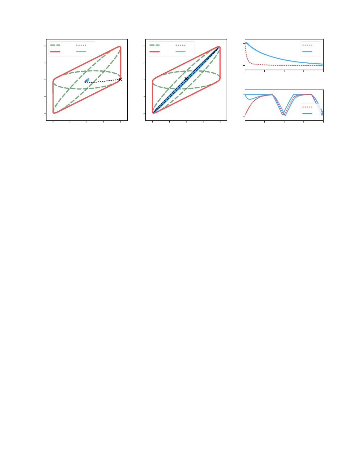
Rob ust Estimator -Based Safety V erification: A V ector Norm A pproach Binghan He 1 , Gray C. Thomas and Luis Sentis Accepted for publication in American Control Conference (A CC) ©2020 IEEE. Personal use of this material is permitted. Permission from IEEE must be obtained for all other uses, in any current or future media, including reprinting/republishing this material for advertising or promotional purposes, creating ne w collective works, for resale or redistribution to servers or lists, or reuse of any copyrighted component of this work in other works. DOI: 10.23919/ACC45564.2020.9147276 Abstract — In this paper , we consider the problem of verifying safety constraint satisfaction for single-input single-output sys- tems with uncertain transfer function coefficients. W e propose a new type of barrier function based on a vector norm. This type of barrier function has a measurable upper bound without full state av ailability . An identifier -based estimator allows an exact bound for the uncertainty-based component of the barrier function estimate. Assuming that the system is safe initially allows an exponentially decreasing bound on the error due to the estimator transient. Barrier function and estimator synthe- sis is proposed as two con vex sub-problems, exploiting linear matrix inequalities. The barrier function contr oller combination is then used to construct a safety backup controller . And we demonstrate the system in a simulation of a 1 degr ee-of-freedom human–exoskeleton interaction. I . I N T RO D U C T I O N Safe control is mission critical for robotic systems with humans in the loop. Uncertain robot model parameters and the lack of direct human state knowledge bring extra diffi- culty to the stabilization of human–robot systems. Methods such as robust loop shaping [1], [2], [3], model reference adaptiv e control [4] and energy shaping control [5] aim to balance the closed loop stability and performance of physical human robot interaction systems. Howe ver , there is no backup controller if these systems fail to maintain safety , because backup safety controllers require full state av ailability . For systems with direct state measurements, safety is usually verified by a barrier certificate. Similar to a L yapunov function, a barrier function or barrier certificate decreases at the boundary of its zero le vel set [6]. While barrier certificate can be synthesized automatically through sum- of-squares (SoS) optimization [7], a more ambitious goal is to combine the synthesis of the barrier function and the controller together through a control barrier function [8]. V arious methods such as backstepping [9] and quadratic programming [10], [11] create control barrier functions to ensure output and state constraint satisfaction while other methods such as semidefinite programming [12] aimed to also include input saturation. Safety warranties can also be considered a problem of finding an in v ariant set of the system which is also a subset the safe region in the state space. This allows us to consider using the synthesis of a quadratic L yapunov function subject This work was supported by the U.S. Government and N ASA Space T echnology Research Fellowship NNX15AQ33H. W e thank the members of the Human Centered Robotics Lab, Univ ersity of T exas at Austin who pro vided insight and expertise that assisted the research. Authors are with The Departments of Mechanical Engineering (B.H., G.C.T .) and Aerospace Engineering (L.S.), Univ ersity of T exas at Austin, Austin, TX. Send correspondence to 1 binghan at utexas dot edu . to the state and input constraints in a series of linear matrix inequalities (LMIs) [13]. T o certify a lar ger safe region, composite quadratic L yapunov functions can combine multiple existing certificates, either centered at the origin [14] or with multiple equilibrium points [15]. The LQR-T ree strategy [16], which could potentially be applied to safety control, creates a series of connected regions of attraction (also known as funnels) using quadratic L yapunov functions for mapping the reachable state space. In [17], a strategy was proposed to observe the safety of a system through its passivity which can be considered as a more conserv ative safety constraint than quadratic L yapunov stability . A state space realization models a physical process if it correctly reproduces the corresponding output for each admissible input [18]. A Luenberger observer [19] asymptot- ically estimates the state of such a model of a linear system with only the direct measurement of input and output. This idea has also been extended for system with nonlinear mod- eling error [20]. For bounded modeling errors, the estimation error con ver ges to a residue set instead of zero [21]. Recently , a method of using sum-of-squares programming [22] aims to optimize the con ver ging rate of a robust state estimation for uncertain nonlinear systems. But the estimated state still cannot be directly used for e valuation of barrier functions until it fully con ver ges. The system could possibly violate the safety constraints before the barrier function estimation becomes valid. In this paper , we aim to close the gap between state estimation and safety assurance for uncertain systems. In order to address the barrier function estimation, we start with an identifier-based state estimator [23] which provides us a state estimate that is linear with the uncertain trans- fer function coefficients. Then, we define a vector norm based on a quadratic L yapunov function such that a triangle inequality can be applied to decompose it into estimated state and estimation error . A con vex polytopic bound on the estimated state is a vailiable through the estimator structure, and an upper bound on the estimation error arises from the con vergence rate of the estimator and initial error . T o obtain a larger safe (state-space) region, we extend this upper bound searching strategy to another vector norm defined based on a composite quadratic L yapunov function [14], whose unit level set is a con vex hull of the unit level sets of multiple quadratic L yapunov functions. Using these vector norms, we derive our proposed barrier functions for uncertain systems with stable static output feedback. The synthesis of an estimator for the proposed barrier functions can be done in a two-step con vex optimization using linear matrix inequalities, first optimizing the barrier function and then optimizing the estimator . This establishes a barrier pair [15], which can be used with a hybrid safety controller to guarantee safety even for arbitrary inputs. In the end, our hybrid safety controller is demonstrated in a simulation of a simple human-exoskeleton interaction model with human stiffness uncertainty and velocity and force limits. I I . P R E L I M I NA R I E S A. Pr oblem Statement Let us consider an n -th order strictly proper uncertain SISO system Σ p with transfer function P ( s ) = y ( s ) u ( s ) = b 1 s n − 1 + · · · + b n − 1 s + b n s n + a 1 s n − 1 + · · · + a n − 1 s + a n , (1) a i ∈ [ ¯ a i , ¯ a i ] , i ∈ { 1, 2, · · · , n } , (2) b j ∈ [ ¯ b j , ¯ b j ] , j ∈ { 1, 2, · · · , n } , (3) where u and y are the input and output of Σ p and i and j are the indices of the polynomial coefficients. A state space realization of (1) can be expressed as ˙ x = A x + b u u , (4) y = c 0 x , (5) where x is the state vector . W e specify ( A , b u , c 0 ) as an n-dimensional observable canonical form with c 0 ∆ = [ 1, 0, · · · , 0 ] . W ith the state space realization in the form of (4), the problem we consider is defined as follows. Pr oblem: Suppose there is exists a stable controller for the parameter uncertain system Σ p which can satisfy constraints x ∈ X and u ∈ U indefinitely for all initial states in X s ⊆ X , find an estimator Σ e that can observe whether the system is inside the safe region X s with direct measurement of only the input u and output y ev en when this controller is not necessarily activ e. B. State Estimation Since only u and y are directly measured, we need to estimate x in (4) to verify safety . According to Lemma 1 in [24], we can select a strictly stable A 0 in observable canonical form such that (4) becomes ˙ x = A 0 x + b y y + b u u , (6) where A in (4) is replaced by A 0 + b y c 0 . Let the characteris- tic equation of A 0 be s n + ˆ a 1 s n − 1 + · · · + ˆ a n − 1 s + ˆ a n . Since ( c 0 , A 0 ) is also a pair in the observ able canonical form, b y and b u are b y = [ ˆ a 1 − a 1 , ˆ a 2 − a 2 , · · · , ˆ a n − a n ] T , (7) b u = [ b 1 , b 2 , · · · , b n ] T , (8) which are either linear with or af fine to the coefficients of the polynomials of P ( s ) in (1). W e estimate x through an identifier-based estimator which includes a pair of sensitivity function filters expressed as ˙ θ y = A T 0 θ y + c T 0 y , ˙ θ u = A T 0 θ u + c T 0 u , (9) where ( A T 0 , c T 0 ) is a controllable pair in the canonical form. Lemma 1: Suppose E y = C − 1 0 Θ T y and E u = C − 1 0 Θ T u where C 0 is the observability matrix of ( c 0 , A 0 ) , and Θ y and Θ u are the controllability matrices of ( A T 0 , θ y ) and ( A T 0 , θ u ) . E y b y + E u b u con verges to x exponentially . Pr oof: This is similar to Lemma 2 in [24]. Notice that C 0 is also the transpose of the controllability matrix of ( A T 0 , c T 0 ) . W e can derive from (9) that ˙ E T y = A T 0 E T y + I y , ˙ E T u = A T 0 E T u + I u . (10) Because A 0 is in a canonical form, it is easy to show that E y A 0 = A 0 E y and E u A 0 = A 0 E u . Therefore, by taking the transpose of (10), we obtain ˙ E y = A 0 E y + I y and ˙ E u = A 0 E u + I u . If we define ˆ x ∆ = E y b y + E u b u , then ˙ ˆ x = A 0 ˆ x + b y y + b u u . Since A 0 is strictly stable, we hav e x = ˆ x + e where e = e A 0 t ( x ( 0 ) − ˆ x ( 0 ) ) . Notice that the dynamics of ˆ x can also be expressed as ˙ ˆ x = A ˆ x + b y ( y − c 0 ˆ x ) + b u u , (11) which is a Luenberger observer of (4). Howe ver (11) cannot be directly implemented because of the uncertainty in b y and b u . The identifier-based estimator in (9) provides us a con vex hull containing the estimated state vector ˆ x , ˆ x ( b y , b u ) ∈ Co  E y      ˆ a 1 − a 1 ˆ a 2 − a 2 . . . ˆ a n − a n      + E u      b 1 b 2 . . . b n      , a i ∈ { ¯ a i , ¯ a i } , b j ∈ { ¯ b j , ¯ b j } , for i , j = 1, 2, · · · , n  . (12) Because of the initial estimation error e 0 ∆ = x ( 0 ) − ˆ x ( 0 ) , any barrier function B ( x ) aiming to constrain the system inside the safe region X s cannot be directly bounded using ˆ x ( b y , b u ) . Instead, our goal is to find an upper bound for the barrier function using both ˆ x ( b y , b u ) and e 0 . C. V ector Norm Function In order to upper bound the barrier function proposed later in this paper , we recall the following two properties of a vector norm function. Lemma 2: For every vector x in some vector space within R n , let k ·k be a scalar function of x with the following properties. (a) 0 < k x k < ∞ except for k x k = 0 at the origin. (b) k λ x k = | λ | k x k for all λ ∈ R . Then k ·k satisfies (c) k x + y k ≤ k x k + k y k if and only if Ω ∆ = { x | k x k ≤ 1 } is con vex. These properties (a), (b) and (c) in Lemma 2 are also called the three characteristic properties of a vector norm. Lemma 3: Let k· k be a vector norm function satisfying (a), (b) and (c) in Lemma 2. Suppose there is a vector x 0 = ∑ N j = 1 γ j x j with ∑ N j = 1 γ j = 1 , 0 ≤ γ j < 1 for all j = 1, 2, · · · , N and k x 0 k = λ . Then there exists an index j such that k x j k ≥ λ . Pr oof: Suppose that k x j k < λ for all j = 1, 2, · · · , N . Based on (b) in Lemma 2, we have k γ j x k = | γ j |k x k for all j = 1, 2, · · · , N . Applying (c) in Lemma 2 to k x 0 k we get k x 0 k =   N ∑ j = 1 γ j x j   ≤ N ∑ j = 1 γ j k x j k < N ∑ j = 1 γ j λ = λ , (13) which contradicts k x 0 k = λ . I I I . B A R R I E R E S T I M AT I O N The triangle inequality of vector norms allows us to de- compose the state x into the estimated state ˆ x and estimation error e . While we do not know x , we kno w ˆ x and can bound e within a decaying windo w—allowing us to extend barrier pairs [15] to systems without full state av ailability . A. Norm of Quadratic L yapunov Function Let us define a quadratic L yapunov function as V q ( x ) = x T Q − 1 x where Q is a positive definite matrix. W e can form a vector norm using its square root, k x k q ∆ = V 1 2 q ( x ) , (14) because V q ( x ) is positiv e definite, V q ( λ x ) = λ 2 V q ( x ) and the unit lev el set of V ( x ) is con vex. For a gi ven pair of E y and E u , we can deri ve from Lemma 3 that the maximum value of k ˆ x k q occurs at one of vertices of the conv ex hull in (12). Theor em 1: If a strictly stable matrix A 0 in (6) and (9) satisfies A 0 Q + Q A T 0 + 2 α Q  0, (15) then for all t ≥ 0 there exists an i ∈ { 1, · · · , N } such that k x k q ≤ k ˆ x ( b yi , b ui ) k q + e − α t k e 0 k q , (16) where ˆ x ( b yi , b ui ) for i = 1, 2, · · · , N are the all vertices of (12). Pr oof: From Lemma 2, we have k x k q ≤ k ˆ x k q + k e k q . The time deriv ativ e of V q ( e ) can be expressed as ˙ V q ( e ) = e T ( Q − 1 A 0 + A T 0 Q − 1 ) e = e T Q − 1 ( A 0 Q + Q A T 0 ) Q − 1 e . (17) By substituting (15), ˙ V q ( e ) ≤ − 2 α V q ( e ) which guarantees that V q ( e ) ≤ e − 2 α t V q ( e 0 ) . Therefore, k e k q ≤ e − α t k e 0 k q . T ogether with Lemma 3, we have (16). This Theorem 1 provides an upper bound on k x k q which is a vailable in that it be calculated from ˆ x and e 0 for all t ≥ 0 . B. Norm of Composite Quadratic L yapunov Function In order to obtain a lar ger safe re gion X s , a composite quadratic L yapunov function is considered. For multiple − 1.0 − 0.5 0.0 0.5 1.0 x 1 − 1.0 − 0.5 0.0 0.5 1.0 x 2 Ω q j Ω c Fig. 1. A unit ball Ω c of k x k c equiv alent to the conve x hull of the ellipsoidal unit balls Ω q j of three different k x k q j . different quadratic L yapunov functions defined with positi ve- definite matrices Q 1 , Q 2 , · · · , Q n q , a composite quadratic L yapunov function [14] is defined as V c ( x ) ∆ = min γ x T Q − 1 ( γ ) x , (18) Q ( γ ) ∆ = n q ∑ j = 1 γ j Q j , (19) where ∑ n q j = 1 γ j = 1 and γ j ≥ 0 for all j = 1, 2, · · · , n q . The unit lev el set of V c ( x ) is the con vex hull of all the unit level sets of V q j ( x ) = x T Q − 1 j x for j = 1, 2, · · · , n q and is therefore also a conv ex shape (see Fig. 1). Since V c ( x ) is positi ve definite and V c ( λ x ) = λ 2 V c ( x ) , we can use Lemma 2 to define the “composite” vector norm, k x k c ∆ = V 1 2 c ( x ) . (20) Theor em 2: For all j = 1, 2, · · · , n q , if a strictly stable matrix A 0 in (6) and (9) satisfies A 0 Q j + Q j A T 0 + 2 α Q j  0, (21) then for all t ≥ 0 there exists an i ∈ { 1, · · · , N } such that k x k c ≤ k ˆ x ( b yi , b ui ) k c + e − α t k e 0 k c (22) where ˆ x ( b yi , b ui ) for i = 1, 2, · · · , N are the all vertices of (12). Pr oof: As in Theorem 1. Therefore, an upper bound on k x k c can be calculated using ˆ x and e 0 for all t ≥ 0 . C. Barrier P airs Definition 1 (See [15]): A Barrier P air is a pair of func- tions ( B , k ) with two following properties: (a) − 1 < B ( x ) ≤ 0, u = k ( x ) = ⇒ ˙ B ( x ) < 0 , (b) B ( x ) ≤ 0 = ⇒ x ∈ X , k ( x ) ∈ U , where (a) and (b) are also called in variance and constraint satisfaction. W e can now introduce two barrier pairs using our vector norms and static output feedback controller . Pr oposition 1: Suppose V q is a quadratic L yapunov func- tion for system of (4) and (5) with a static output feedback u = k y and Ω q is a unit ball of k x k q defined as (14). If Ω q ⊆ X ∩ { x | c 0 x ∈ k − 1 U } , (23) then ( k x k q − 1, k y ) is a barrier pair . Pr oof: Let B q ( x ) = k x k q − 1 . Its time deriv ative is ˙ B q ( x ) = 1 2 k x k − 1 q ˙ V q . (24) Since k x k − 1 q > 0 and ˙ V q < 0 when − 1 < B q ( x ) ≤ 0 , ( B q ( x ) , k y ) satisfies (a) in Definition 1. From (23), we also hav e (b) in Definition 1 satisfied. Pr oposition 2: Suppose V c is a composite quadratic L ya- punov function defined as (18) and (19) for the system of (4) and (5), with static output feedback u = k y and that Ω c is a unit ball of k x k c defined as in (20). If we have Ω c ⊆ X ∩ { x | c 0 x ∈ k − 1 U } , (25) then ( k x k c − 1, k y ) is a barrier pair . Pr oof: As in Proposition 1. As in (16) and (22), upper bounds of the barrier functions of these two barrier pairs can be calculated using ˆ x and e 0 for all t ≥ 0 . I V . S Y N T H E S I S Both barrier functions B c ( x ) ∆ = k x k c − 1 and their identifier-based estimators can be synthesized with LMIs, through the sub-problem of synthesizing B q ( x ) ∆ = k x k q − 1 . A. Q j Synthesis W ith static output feedback, the closed loop system of (4) is still a polytopic linear differential inclusion (PLDI) model [13] ˙ x ∈ A c x with A c = Co       0 1 0 . . . . . . 0 0 1 0 0 · · · 0      −      a 1 a 2 . . . a n      c 0 +      b 1 b 2 . . . b n      k c 0 , a i ∈ { ¯ a i , ¯ a i } , b j ∈ { ¯ b j , ¯ b j } , for i , j = 1, 2, · · · , n  . (26) Supposing that X and U can be described (perhaps conser- vati vely) as X = { x : | f i x | ≤ 1, i = 1, 2, · · · , n f } , (27) U = { u : | u | ≤ ¯ u } , (28) they can be enforced by LMIs f i Q j f T i ≤ 1, ∀ i = 1, 2, · · · , n f , (29) c 0 Q j c T 0 ≤ ¯ u 2 k 2 . (30) T o synthesize Q j , we maximize the width of the unit ball of x T Q − 1 j x along some state space direction x j by minimizing Σ p ˙ x = A x + b u u y = c 0 x Σ s u = ˆ u or u = k y Σ e ˙ θ y = A T 0 θ y + c T 0 y ˙ θ u = A T 0 θ u + c T 0 u ˆ x = E y b y + E u b u ˆ u u y ˆ B y y Fig. 2. Block diagram consisting of plant Σ p , estimator Σ e and hybrid safety controller Σ s . u = ˆ u u = k y start ∃ ˆ B ( b yi , b ui ) ≥ ¯ B ∀ ˆ B ( b yi , b ui ) ≤ ¯ B Fig. 3. Switching logic of hybrid safety controller Σ s . ρ j subject to the following LMI " ρ j x T j x j Q j #  0, (31) such that the optimization sub-problem becomes minimize Q j ρ j subject to (29) , (30) , (31) , Q j  0, A ci Q j + Q j A T ci + 2 α 0 Q j  0, ∀ i = 1, 2, · · · , N . (32) where A ci for i = 1, 2, · · · , N are the all vertices of (26). A positiv e value of α 0 is used to guarantee a minimum exponential decay rate for k x k c . B. A 0 Synthesis While it is simple to specify an A 0 in (6) with a fast decay rate of e (choosing big negati ve-real-part eigenv alues), this does not necessarily improv e the value of α in (22). T o synthesize an A 0 in the set of matrices in observable canonical form O ⊂ R n × n we directly optimize for α : maximize A 0 ∈ O α subject to A 0 Q j + Q j A T 0 + 2 α Q j  0, ∀ j = 1, 2, · · · , n q , (33) knowing that a solution α ≥ α 0 will exist. (Any A 0 in the con vex hull of (26) is guaranteed to satisfy the constraints in (33) with a decay rate of α 0 .) C. Hybrid Safety Contr oller T o enforce safety satisfaction on a potentially unsafe input ˆ u , we can estimate the barrier function as ˆ B c ( b y , b u ) ∆ = k ˆ x ( b y , b u ) k c + e − α t k e 0 k c − 1. (34) W ith this estimate, we can design a hybrid safety controller Σ s which decides whether to apply either ˆ u or k y (that is, the safety backup control law) as the input in order to keep B c ≤ 0 (see Fig. 2) and therefore guarantee safety . According to Theorem 2, system Σ p is guaranteed to be safe if ˆ B c ( b yi , b ui ) ≤ 0 for all vertices ˆ x ( b yi , b ui ) of con ve x hull (12). Therefore, the switching logic for Σ s defined in Fig. 3, which introduces two near-zero thresholds ¯ B and ¯ B (with − 1 < ¯ B < ¯ B ≤ 0 ), will result in robust safety . V . E X A M P L E T o illustrate robust barrier function estimation and hybrid safety control, we introduce a simplified human-exoskeleton interaction model. As shown in Fig. 4, this model is a mass-spring-damper with uncertain human stiffness k h , the exoskeleton damping b e , and exoskeleton inertia m e . A. Human-Exoskeleton Interaction Model The e xoskeleton plant can be e xpressed as a transfer function P ( s ) = y ( s ) u ( s ) = k h m e s 2 + b e s + k h (35) where the input u is the actuator force exerted and the output y ∆ = k h ( x e − x h ) is the contact force between human and exoskeleton. Although the contact force and the exoskeleton position, x e , can be measured, the reference position, x h , of the human spring is not a vailable because of the unknown stiffness. Suppose that the uncertain value of k h is in the range from 4 to 12 and that the value of b e is 12. W e can express the closed loop A c matrix set with static output feedback as a con vex hull A c = Co   − 12 1 − k h 0  +  0 k h  k c 0 , k h = 4, 12  . (36) And the safety constraints can be defined via the sets X = { [ x 1 , x 2 ] T : | − x 1 + x 2 /12 | ≤ 1 } , U = { u : | u | ≤ 1.2 } , (37) where the output y = x 1 and ˙ y = − 12x 1 + x 2 , so X is constraining the output deriv ativ e | ˙ y | ≤ 12 . B. Simulation W e choose the static output feedback gain k = − 1.2 which is stable, and leads to a human amplification factor of 2.2 and the output constraint | y | ≤ 1 . In Fig. 5, we construct a barrier function B c from two different quadratic L yapunov functions (optimized along directions x j = [ 1, 0 ] T and x j = [ 1, 12 ] T ) generated by synthesis (32) with a shared decay rate of α 0 = 0.50 . Then, an A 0 matrix with a characteristic polynomial s 2 + ˆ a 1 s + ˆ a 2 (with ˆ a 1 = 13.60 and ˆ a 2 = 18.68 ) and a higher decay rate ( α = 0.68 ) is generated from synthesis (33). Notice that the optimal A 0 matrix is not exactly inside the conv ex hull of (36). In the numerical simulation, human stif fness k h = 8 . In our first simulation, we release the system near the boundary of Ω c with zero nominal input. In the second simulation the m e = 1 b e k h u x e x h Fig. 4. Our simplified human–exosk eleton interaction model, a mass- spring-damper system, includes an uncertain human stiffness k h , an ex- oskeleton damping b e , and an exoskeleton inertia m e . system starts at the origin and we apply a nominal input ˆ u which tracks an unsafe reference y trajectory: y ( t ) = 1.2 · sin ( 0.05 · 2 π t ) . In the first test (Fig. 5.a) the static output feedback is alw ays on, to demonstrate the slower decay of ˆ B c ( k h ) . In the second (Fig. 5.b), the static output feedback is turned on when max ( ˆ B c ( k h )) ≥ ¯ B = − 0.01 and is turned off when all v alues of max ( ˆ B c ( k h )) ≤ ¯ B = − 0.02 . This switching logic forces the system to stop near the boundary of Ω c —deviating from the unsafe trajectory to produce a safe output. In both tests, the largest element of ˆ B c ( k h ) con verges to zero slower than the v alue of B c such that max ( ˆ B c ( k h )) ≥ B c , as shown in Fig. 5.c and Fig. 5.d respectively . V I . D I S C U S S I O N Because the estimated barrier function ˆ B c includes the transient term e − α t k e 0 k c , which is initially at a value of 1— indicating our assumption that the system state starts within the safe region—the safety backup controller is always activ e initially . Since our system is modelled as noiseless, this transient decays towards zero and the composite barrier approaches a steady state that robustifies the barrier only against the effect of parameter uncertainty . If there were additional uncertainty in the measurements, for example Gaussian noise, then this transient would asymptotically approach a steady-state non-zero value instead. When the barrier function estimate is near the thresholds, as in Fig. 5.d, the control switches rapidly between ˆ u and k y . The frequency of this switching can be controlled by increasing the gap between ¯ B and ¯ B , which can reduce the risk of activ ating unmodeled high frequency dynamics. If we were to combine the synthesis of the barrier function and estimator together in one optimization, setting α equal to α 0 , the LMIs in (33) would become bilinear matrix inequalities (BMIs). Since the estimator state equation in (11) is in a canonical form, a new variable could be defined using the sufficient condition proposed in [25] to reduce these BMIs to LMIs. Howe ver , this sufficient condition would not always result in a feasible optimization problem. The proposed synthesis strategy can be extended to sys- tems with a pre-specified dynamic output feedback—albeit inefficiently . Though the states of a dynamic output feedback controller are perfectly kno wn, they can also be considered part of the plant and estimated the same way as plant states. Input constraints can be incorporated as state constraints on the part of this composite plant that represents controller states. Then, synthesis (32) and (33) can be applied directly by setting k to be zero. (a) x 2 x 1 − 1.0 − 0.5 0.0 0.5 1.0 − 12 − 6 0 6 12 Ω q j Ω x x ˆ x x 2 (b) x 1 − 1.0 − 0.5 0.0 0.5 1.0 − 12 − 6 0 6 12 Ω q j Ω x x ˆ x (c) (d) t (s) t (s) 0 1 2 3 4 − 1 0 0 5 10 15 20 − 1 0 B c ˆ B c B c ˆ B c Fig. 5. Simulation results. In the fist simulation, the system state is initialized near the boundary of Ω c (phase plot in (a)). The maximum ˆ B c ( k h ) conv erges slower than B c (in (c)). In the second simulation, an unsafe sinusoidal input ˆ u is forced to be safely inside Ω c by a hybrid safety controller (phase plot in (b)). This safety controller activ ates only when max ( ˆ B c ( k h )) u 0 (see (d)). This strategy can also be naturally extended to supervisory control [23] of a family of sub-optimal output feedback con- trollers subject to different subsets of parameter uncertainty by turning (9) into a shared state parameter identifier , as pro- posed in [24]. Substituting for methods such as constrained model reference adaptiv e control [26], [27] and adaptive control barrier functions [28], safety during the parameter adaptation could be enforced by switching to a backup barrier pair which is robust to the full parameter uncertainty . R E F E R E N C E S [1] S. P . Buerger and N. Hogan, “Complementary stability and loop shaping for improved human–robot interaction, ” IEEE T ransactions on Robotics , vol. 23, no. 2, pp. 232–244, 2007. [2] B. He, G. C. Thomas, N. Paine, and L. Sentis, “Modeling and loop shaping of single-joint amplification exoskeleton with contact sensing and series elastic actuation, ” in 2019 American Control Conference (ACC) . IEEE, 2019, pp. 4580–4587. [3] G. C. Thomas, J. M. Coholich, and L. Sentis, “Compliance shaping for control of strength amplification exoskeletons with elastic cuffs, ” in Pr oceedings of the 2019 IEEE/ASME International Conference on Advanced Intelligent Mechatr onics . IEEE and ASME, July 2019, pp. 1199–1206. [4] S. Chen, Z. Chen, B. Y ao, X. Zhu, S. Zhu, Q. W ang, and Y . Song, “ Adaptive robust cascade force control of 1-dof hydraulic exoskeleton for human performance augmentation, ” IEEE/ASME T ransactions on Mechatr onics , vol. 22, no. 2, pp. 589–600, 2016. [5] G. Lv and R. D. Gregg, “Underactuated potential energy shaping with contact constraints: Application to a powered knee-ankle orthosis, ” IEEE Tr ansactions on Control Systems T echnology , vol. 26, no. 1, pp. 181–193, 2017. [6] S. Prajna and A. Jadbabaie, “Safety verification of hybrid systems us- ing barrier certificates, ” in International W orkshop on Hybrid Systems: Computation and Control . Springer, 2004, pp. 477–492. [7] S. Prajna, “Barrier certificates for nonlinear model validation, ” Auto- matica , v ol. 42, no. 1, pp. 117–126, 2006. [8] P . Wieland and F . Allg ¨ ower , “Constructive safety using control barrier functions, ” IF A C Pr oceedings V olumes , vol. 40, no. 12, pp. 462–467, 2007. [9] K. P . T ee, S. S. Ge, and E. H. T ay , “Barrier lyapunov functions for the control of output-constrained nonlinear systems, ” Automatica , vol. 45, no. 4, pp. 918–927, 2009. [10] A. D. Ames, X. Xu, J. W . Grizzle, and P . T abuada, “Control barrier function based quadratic programs for safety critical systems, ” IEEE T ransactions on Automatic Contr ol , vol. 62, no. 8, pp. 3861–3876, 2016. [11] Q. Nguyen and K. Sreenath, “Optimal robust safety-critical control for dynamic robotics, ” International Journal of Robotics Researc h (IJRR), in r eview , 2016. [12] D. Pylorof and E. Bakolas, “ Analysis and synthesis of nonlinear con- trollers for input constrained systems using semidefinite programming optimization, ” in 2016 American Contr ol Conference (ACC) . IEEE, 2016, pp. 6959–6964. [13] S. Boyd, L. El Ghaoui, E. Feron, and V . Balakrishnan, Linear matrix inequalities in system and contr ol theory . Siam, 1994, vol. 15. [14] T . Hu and Z. Lin, “Composite quadratic lyapuno v functions for con- strained control systems, ” IEEE T ransactions on Automatic Contr ol , vol. 48, no. 3, pp. 440–450, 2003. [15] G. C. Thomas, B. He, and L. Sentis, “Safety control synthesis with input limits: a hybrid approach, ” in 2018 Annual American Contr ol Confer ence (A CC) . IEEE, 2018, pp. 792–797. [16] R. T edrake, I. R. Manchester, M. T obenkin, and J. W . Roberts, “Lqr- trees: Feedback motion planning via sums-of-squares v erification, ” The International Journal of Robotics Researc h , vol. 29, no. 8, pp. 1038– 1052, 2010. [17] B. Hannaford and J.-H. Ryu, “Time-domain passivity control of haptic interfaces, ” IEEE T ransactions on Robotics and Automation , v ol. 18, no. 1, pp. 1–10, 2002. [18] A. Morse, “Representations and parameter identification of multi- output linear systems, ” in 1974 IEEE Conference on Decision and Contr ol including the 13th Symposium on Adaptive Pr ocesses . IEEE, 1974, pp. 301–306. [19] D. G. Luenberger , “Observing the state of a linear system, ” IEEE transactions on military electr onics , vol. 8, no. 2, pp. 74–80, 1964. [20] M. Zeitz, “The extended luenberger observer for nonlinear systems, ” Systems & Control Letters , vol. 9, no. 2, pp. 149–156, 1987. [21] M. Corless and J. T u, “State and input estimation for a class of uncertain systems, ” Automatica , vol. 34, no. 6, pp. 757–764, 1998. [22] D. Pylorof, E. Bakolas, and K. S. Chan, “Design of robust lyapunov- based observers for nonlinear systems with sum-of-squares program- ming, ” IEEE Control Systems Letters , v ol. 4, no. 2, pp. 283–288, 2019. [23] A. S. Morse, “Supervisory control of families of linear set-point controllers-part i. exact matching, ” IEEE transactions on Automatic Contr ol , vol. 41, no. 10, pp. 1413–1431, 1996. [24] A. Morse, “Global stability of parameter-adaptiv e control systems, ” IEEE T ransactions on Automatic Contr ol , vol. 25, no. 3, pp. 433–439, 1980. [25] C. A. Crusius and A. T rofino, “Sufficient LMI conditions for output feedback control problems, ” IEEE T ransactions on Automatic Control , vol. 44, no. 5, pp. 1053–1057, 1999. [26] E. Arabi, B. C. Gruenwald, T . Y ucelen, and N. T . Nguyen, “ A set- theoretic model reference adaptive control architecture for disturbance rejection and uncertainty suppression with strict performance guaran- tees, ” International Journal of Control , vol. 91, no. 5, pp. 1195–1208, 2018. [27] A. LAfflitto, “Barrier lyapunov functions and constrained model reference adaptiv e control, ” IEEE Control Systems Letters , vol. 2, no. 3, pp. 441–446, 2018. [28] A. J. T aylor and A. D. Ames, “ Adaptive safety with control barrier functions, ” arXiv preprint , 2019.