Regularity of solutions of the isoperimetric problem that are close to a smooth manifold

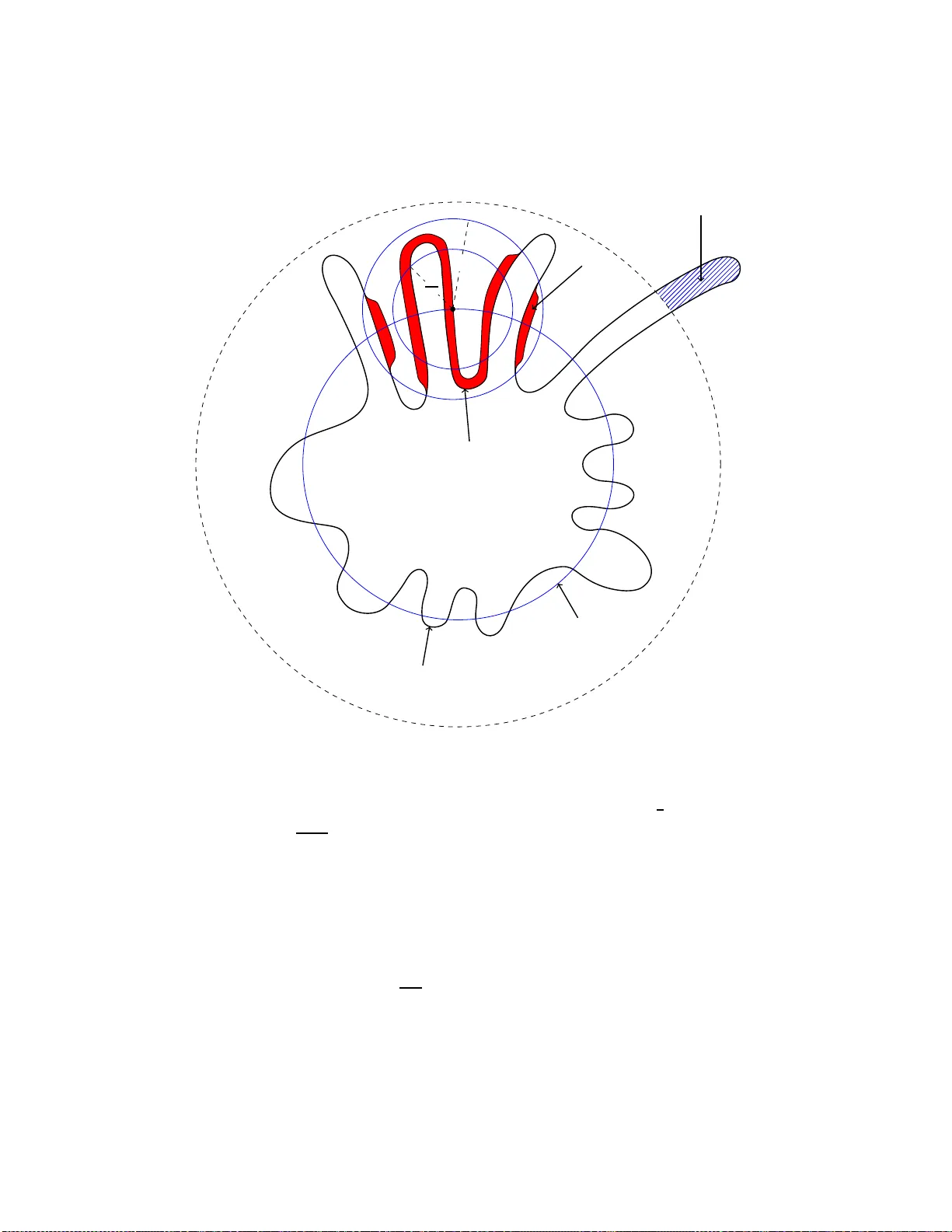
Regularit y of isop erimetric regions that are close to a smo oth manifold ∗ Stefano Nardulli No v em b er 1, 2018 Con ten ts 1 In tro duction 2 1.1 A regularit y theorem . . . . . . . . . . . . . . . . . . . . 2 1.2 Previous results . . . . . . . . . . . . . . . . . . . . . . . 5 1.3 Some applications of Th eo rem 1 . . . . . . . . . . . . . 5 1.4 Sk etc h of the pr oof of Theorem 1 . . . . . . . . . . . . . 5 1.5 Plan of the article . . . . . . . . . . . . . . . . . . . . . 7 1.6 Ac kn owledgemen ts . . . . . . . . . . . . . . . . . . . . . 8 2 Regularit y Theory 8 2.1 Notatio ns . . . . . . . . . . . . . . . . . . . . . . . . . . 8 2.2 Mean curv ature vec tor based on an hypers urface . . . . 9 2.3 Allard’s Regularit y Theorem . . . . . . . . . . . . . . . 17 2.4 First V ariation of isop erimetric regions . . . . . . . . . . 24 2.5 Riemannian Monotonicit y F orm ula u sing isometric em- b edding . . . . . . . . . . . . . . . . . . . . . . . . . . . 26 3 The N ormal Graph Theorem 28 3.1 Sk etc h of the Pro of of Th e orem 3.1 . . . . . . . . . . . . 29 3.2 A priori estimates on mean curv ature . . . . . . . . . . . 30 3.3 V olume of the In tersection of a smo oth h yp ersurf a ce with a ball of the ambien t Riemannian manifold . . . . . . . 33 3.4 Comp ensation of V olume Pro cess . . . . . . . . . . . . . 36 ∗ W ork supp orted by the grant ”Borse p er l’Estero” of I ND A M 1 2 3.5 Comparison of t he area of the b oundary of an isop erimet- ric domain with th e area of a p erturb ation with constant v olume . . . . . . . . . . . . . . . . . . . . . . . . . . . . 39 3.6 Conﬁnement of an Isop erimetric Domain by Monotonic- it y F orm ula . . . . . . . . . . . . . . . . . . . . . . . . . 43 3.7 Alternativ e pro of of co nﬁnement u nder weak er b ounded geometry assumptions . . . . . . . . . . . . . . . . . . . 46 3.8 Pro of of Theorem 3.1 . . . . . . . . . . . . . . . . . . . . 56 3.9 Some reﬁned mean cu r v ature estimates . . . . . . . . . . 64 4 Pro o f of Theorem 1 : Normal Graph Theorem wit h v ari- able met ric s 66 Bibliograph y 75 1 In tro duction 1.1 A regularity theorem In this article we giv e some regularit y results for the b ound ary of isop eri- metric regions in a smo oth complete Riemann i an manifold with v ari- able metric using th e theory of regularit y of Allard. In the r ema ining part of this p a p er w e alw a ys assum e that all the Riemannian m a n- ifolds ( M , g ) considered are smo oth with sm ooth Riemannian metric g . M n k will d enot e th e simp ly conn e cted sp a ce form of constan t sec- tional curv ature k . F or ev ery m ∈ N , w e d enot e b y H m g , the m - dimensional Hausdorﬀ measure asso cia ted to the metric space ( M , d g ), where d g is the canonical length space metric asso ciated to g , i.e., d g ( x, y ) := in f { l g ( γ ) : γ is a piecewise C 1 curv e joining x to y } , l g ( γ ) rep- resen ts the length of the curve γ w ith resp ect to the Riemannian m e tric g . V ol g = H n g will denote th e canonical Riemannian m e asure in duced on M by g , by A g w e will d e note often H n − 1 g , M g indicates the mass of a current, the notation here is the standard one of F ederer’s b o ok [ F ed69 ]. When it is already clear from the context , explicit men tion of the metric g w ill b e su ppressed. All alo ng this text w e will encoun ter a lot of constants that d e p ends on v arious geometrical qu a n tities and the metric g , when a constan t c dep ends on th e metric g and on its ﬁrst and/or second deriv ativ es con tin uously , w e will denote this fact b y writing c = c ( g , ∂ g, ∂ 2 g ). In what follo w we will also b e concerned with isop erimetric r e gions that are close to a ﬁxed open relativ ely compact set B ⊆ M with smo ot h b oundary ∂ B . As a consequence of this fact 3 w e need to consider also the depen dence on B ⊆ M and a ﬁxed once at all ξ ∈ X ( M ), where X ( M ) is the set of smo ot h vecto r ﬁelds deﬁn e d on M n , these ob jects d e p ending only on the diﬀerentia ble str ucture of M n (that is considered ﬁxed in this w ork) without an y referen c e to a Riemannian metric. T o deal w it h the case of v ariable metrics w e will use the celebrated Nash’s isometric embed ding Theorem. So in gen- eral our constants c will b e of t w o kinds. Th e constants of the ﬁr st kind are of the form c = c ( B , ξ , g, ∂ g , ∂ 2 g ) when they do not dep end on the Nash’s isometric im b edding in some higher dimens i onal Euclidean space i g : ( M n , g ) → ( R N , δ ) for some N > n , wher e δ is the Eu- clidean canonical metric. The constan ts are of the second kind when they dep end on a Nash’s isometric imbedd ing. In this latter case we write c = c ( B , ξ , i g , g , ∂ g , ∂ 2 g ). Ho w ev er, as w e w i ll see later in Sec- tion 4 , C 2 dep endence on i g means to dep end C 4 on the metric so in general another kind of typical constan ts th at we will encounte r is c = c ( B , ξ , i g , g , ∂ g , ∂ 2 g ) = c ( B , ξ , g , ∂ g , ∂ 2 g , ∂ 3 g , ∂ 4 g ). Deﬁnition 1.1. L et ( M , g ) b e a smo oth (p ossibly non-c omplete) R ie- mannian manifold of dimension n . We denote by τ M the class of r elatively c omp act op en sets of M with C ∞ b oundary. The function I ( M ,g ) : [0 , V ol g ( M )[ → [0 , + ∞ [ deﬁne d by I ( M ,g ) ( v ) := inf { A g ( ∂ Ω) | Ω ∈ τ M , V ol g (Ω) = v } , (1) is c al le d the isop erimetric pr oﬁle function (shortly the isop erimet- ric p r oﬁle ) of the manifold M . We deﬁne an isop erimetric r e gion for volume v as an n -dimensional inte gr al normal curr ent T , such that M g ( T ) = v and M g ( ∂ T ) = I ( M ,g ) ( v ) . The r e gularit y theory for minimizing current s, inaugurated by Ennio De Giorgi in co dimension 1 (see for example [ DGCP72 ]), F ederer and Fleming in a n y codimen s i on, and fully dev elop ed in the w ork of Alm- gren and Allard, sho w s that isop erimetric regions are almost smo oth. Precisely , they are su bmanifolds with smo o th b ound ary on the comple- men t of a singular set of co d imension at least equal to 7 [ Alm76 ]. In co dimension 1 one ca n compare with [ GMT83 ] in whic h the theory of ﬁnite p erimeter s e ts is adopted. O n the other hand, for manifolds M n of dimension n ≥ 8 there can b e minimizing cur ren ts whith non-smo oth b oundary (see [ Alm76 ], [ Mo r03 ], [ BGG69 ]). The ﬁrst resu lt along these lines, d ue to Bom bieri, De Giorgi, and Giusti [ BGG69 ], sho ws that the cone C := { ( x, y ) ∈ R 4 × R 4 : | x | = | y |} , as conjectured by James Simons is singular at th e origin and has minimal area in R 8 . In ev ery 4 ball of R n , suc h a cur r en t is a m in ima l h yp ersur f a ce. Coming bac k to the isop erimetric problem, consid er a p oin t p b elonging to the sup p ort of the b oundary of the curren t T , p ∈ spt ( ∂ T ), for some isop e rimetric region T , then th e tangen t cone of ∂ T at p h a v e to b e area minimizing in T p M n . If the p oint p is regular th e n the tangent cone of ∂ T at p is an h yp erplane. If p is a singular p oin t the tangen t cone at p could b e a gen u i ne co ne. In fact, th er e are examples with non v oid singular part, for more details ab out this matter we recommend the lect ure of Prop o- sition 3 . 5 of [ Mor03 ] in whic h is p ro v ed th at if T is an isop erimetric region p ∈ ∂ T and the tangen tial tangen t cone of ∂ T at p is a hyp er- plane then p is a regular p oin t. Almgren’s Theorem is thus optimal. Therefore, additional conditions are required to get more regularit y in higher dimension. The aim of this article is to sho w in Theorem 1 that an isop erimetric region, suﬃcien tly close in the ﬂat norm to a domain B with smo oth b oundary ∂ B , is also sm ooth and v ery close to B in the C 2 ,α top olo gy and eve ry α ∈ ]0 , 1[. F or further applications of this theorem, we also allo w th a t th e Riemannian metric g of M n to b e v ariable. W e refer the reader to the last Section 4 for the pr ecise meaning and deﬁnitions required to state our main Theorem 1 , esp ecially Deﬁnitions 4.2 and 4.3 of top ologi es. Theorem 1. L et ( M n , p, g ∞ ) b e a p ointe d Riemannian manifold of class C ∞ with b ounde d ge ometry, g j a se que nc e of R iemannian met- rics of class C ∞ c onver ging to g ∞ in the ﬁne C 4 -top olo gy or such that ( M n , p, g j ) c onver ges to g ∞ in the usual p ointe d C 4 -top olo gy. L et B b e an op en r elatively c omp act domain of M with smo oth b oundary ∂ B . Consider T j a se quenc e of isop erimetric r e gions of ( M n , g j ) such that M g ∞ ( B − T j ) → 0 , (2) wher e M g ∞ denotes the mass of a curr ent in the metric g ∞ . Then ∂ T j is the gr aph i n normal exp onential c o or dinates of a function u j on ∂ B . F urthermor e, f o r al l α ∈ ]0 , 1[ , u j ∈ C 2 ,α ( ∂ B ) and || u j || g ∞ ,C 2 ,α ( ∂ B ) → 0 . If the c onver genc e of the metric is in the ﬁne C m,α -top olo gy then we also have || u j || g ∞ ,C m +1 ,α ( ∂ B ) → 0 . Remark 1.1. In the assumptio ns of The or em 1 , r ather than ( 2 ) we c an use the fol lowing e qui va lent c ondition V g j ( B − T j ) → 0 . Remark 1.2. Notic e that || u j || g ∞ ,C 2 ,α ( ∂ B ) → 0 is e qu ival ent to || u j || g j ,C 2 ,α ( ∂ B ) → 0 . 5 Remark 1.3. Observe that, sinc e ∂ B is c omp act the sp ac es C 2 ,α ( ∂ B ) ar e indep e nd ent of the metric g , altho ugh the norm || u j || g ,C 2 ,α ( ∂ B ) de- p ends on g . 1.2 Previous results W e can ﬁ nd a particular case of Theorem 1 in the article [ MJ00 ] of Da vid L. John s o n and F. Morgan, f rom whic h we took a lot of in spiratio n. Indeed, these authors sh ow that in a compact manifold isop erimetric regions f or s m a ll volumes are close to small geod esic balls. On e can also consult Theorem 5 of [ Ros05 ] for analo gous results in the case of a compact Riemannian manifold, but with a diﬀerent pro of. Here we follo w the s a me ideas of [ MJ00 ] adapted to our more general situation, pa ying atten tion to giv e intrinsic metric pr oofs from w hic h ve ry accurate estimates of the C 2 ,α norms and their dep endence on the geometric b ounds of M and on the geometric b ounds of the isometric im b eddings ∂ B ֒ → M ֒ → R N are giv en. 1.3 Some applications of Theorem 1 F rom Theorem 1 , we can argue that if, for a ¯ v > 0, all the isop erimet- ric regions in v olume ¯ v are smo oth, then the isoperimetric regions for v olumes v close to ¯ v are smo oth to o. Under this condition, w e could b e able to reduce the isop erimetric problem for v olumes close to ¯ v to a v ariational problem in ﬁnite dimens i on, as dev elop ed in [ Na r09 ] and [ Nar14b ] und er small v olumes assump tions. An anal ogous program is carried out in a separate pap er see [ GNP09 ] Lemma 6. In [ Nar09 ] and [ Nar14b ] w e us ed Theorem 1 , for showing that for sm a ll volumes the isop erimetric regions are pseudo-bub bles. But the range of app l ication of this theorem and its straigh tforw ard generaliza tions is muc h wider. 1.4 Sk etch of the pro of of Theorem 1 First, assume th a t the metric is ﬁ xed, i.e., g j = g , f o r ev ery j . W e mak e essen tial use of Allard’s regularit y theorem, see [ All72 ], Theorem 8 . 1, whic h states that, if a v arifold V = ∂ T ∋ a , h a s in a ball B ( a, r ), a w eigh t || V || ( B ( a, r )) suﬃciently close to ω n − 1 R n − 1 (where ω n − 1 is the v olume of the unit ball of R n − 1 ), and con trolled ﬁrst v ariation (i.e., mean curv atur e ) in suitable L p -norm, then V is, lo cally , the graph of a function u ∈ C 1 ,α . A regularit y theorem for elliptic partial diﬀerenti al equations and a b o ot strap argum e n t imply that u ∈ C ∞ , and also giv e upp er b ounds f o r || u || C 2 ,α , via Sc h auder estimate s. 6 In order to sho w that ∂ T j satisﬁes the conditions of Allard’s regular- it y theorem, we compare ∂ T j to suitably c hosen deformations with ﬁxed enclosed vo lume. Th is is th e matter in which is in vol v ed sub sec tion 3.4 . Unfortunately for our purp oses, Allard’s th e orem is stated in Eu- clidean sp ac es, h ence w e ha ve to give a Riemannian version via isometric em b eddin g of Riemannian manifolds in Eu clidean spaces. F u rthermore w e need to con trol the second fu ndamen tal form of the isometric em- b eddings relativ e to diﬀerent metrics on M . T o mak e this p ossible we use a ﬁ ne analysis of the pr oof of the Nash’s isometric embedd i ng the- orem that M. Gromo v did in [ Gro86b ], this highligh ts the fact that free isometric em b eddin gs can b e c hosen to dep end cont in uously on the metric. It is w orth n o ting her e that w e follo w the scheme of the proof of T heo rem 2.2 [ MJ00 ], with th e diﬀerence that our con text is more general b ecause we consider arb itrary v olumes instead that only small v olumes, noncompact manifolds instead of compact ones and the p roofs are made in trinsic as we can, when in the pap er [ MJ00 ] all is d on e us- ing an isometric emb ed ding of a compact manifold. Moreo v er w e mak e an extra eﬀort to ﬁnd eﬀectiv e b ounds for the co nstan ts inv olv ed and some impr o v ed arguments and some details that in [ MJ00 ] are not men- tioned, esp ecially the w ay in whic h constan ts are calculate d. In section 2.2 exp licit calculations of the mean cur v ature op erat or of a normal graph ov er a sm ooth ( n − 1)-dimensional su b manifold are done. Lemma 3.1 on how to b ound u niformly the curv atures is lik e in Theorem 2.2 of [ MJ00 ] with the suitable m o diﬁcations requir ed to ﬁt the case of a noncompact manifold. The comp ensation Lemma 3.3 from Section 3.4 is n e w in the literature f o r the intrinsic metric geometry con text and b ecause it is done in a s m a ll ball cen tered on the b oundary of the ﬁxed domain B , r a ther th a n on the b oundary of T . This features al lo ws us to a void the classical dep endence of the constan t measurin g the d isto r- tion of area, on T . W e w ant that the constants inv olv ed d epend s ju st on B , uniformly on T , for v alues of V ol g ( B ∆ T ) smaller than a con- stan t th at dep ends just on B , and the b ounds of the geometry of M that in turn dep end only on g , ∂ g , ∂ 2 g . As a consequence of Lemma 3.3 w e h av e Lemma 3.7 that p ermits to c hec k one of the h yp othesis of th e Allard’s regularit y Theorem, the intrinsic feature of these argu m e n ts is also new. T h e conﬁnement Lemma 3.8 v ia th e monotonicit y formula I did n o t ﬁnd in the literature but it is classical in the Eu c lidean case and p erhaps it already exists for Riemannian manifolds at least f o r minimal submanifolds using Nash’s em b edding Theorem. An alternativ e p roof of Lemma 3.8 is that of the conﬁ n emen t Lemma 3.11 , whic h is inspired b y argumen ts on boun dedness of isop erimetric regions in Euclidean space 7 that can b e found in [ Mor94 ] com b ined with the tec hn ic al comp ensation Lemma 3.3 , and it is new in this form. The main diﬃcult y encountered to adapt the Euclidean argument of [ Mor94 ] to the Riemannian b ounded geometry case consists in u sing an Euclidean t yp e isop erimetric in e qual- it y for small v olumes, bu t ju s t with th is w e only pro d uced Theorem 3 of [ Nar14a ]. T o obtain the full generalit y of Lemma 3.11 w e need the tec hn ical Lemma 3.3 th at p ermits us to con trol the v ariation of the p erimeter of a deformation of v olume ∆ v of T , | ∆ A | by the qu a n tit y c ( n, k , v 0 , B , g , ∂ g , ∂ g 2 )∆ v . Ho w to apply the Allard’s regularit y theo- rem k eeping trac k of the constan ts and the wa y in whic h they dep end on the geometry of the noncompact manifold and on B , I did not ﬁnd in the literature. The Sc h auder’s estimates are classical and Hopf comparison theorems are classical. I p ut all the d e tails required in our con text for completeness and again to k eep trac k of th e constan ts and the quantiti es on wh ic h they dep end in view of th e subsequent application to the case of v ariable metrics. All these features mak e the argumen ts a v ailable for the case of v ariable m e trics, arbitrary v olumes, in trinsically without us - ing an em b edding of M n in to some higher dimensional Euclidean R N . Unfortunately to ac h ie v e this p rog ram I need a v er s i on of the Allard regularit y results state d in th e Riemann ia n case, k eeping trac k of how the constan ts dep end on geometric quant ities. This is a task that I did not wr i te up b ecause the d e tails are cu mb ersome. On the other hand, using the r e mark of Gromo v ab out th e Na sh em b edding T heorem and k eeping trac k of the constan ts inv olv ed I can ov ercome this diﬃculty pa ying the p r ic e of lo osing the optimal C 2 con vergence of th e metrics in fa vor of the stronger C 4 con vergence . T he reader is invited to compare the last p age f or more details ab out this p oin t. 1.5 Plan of the article 1. In su bsect ion 2.2 a u se ful p urely diﬀerent ial geometric formula for the mean curv ature op erator of a normal graph is giv en . S e ction 2 pro vides Riemann ian v ersions of three classical results of geometric measure theory: Allard’s regularit y theorem, the link b et ween ﬁrst v ariation and mean curv ature in the case of currents and v arifolds, the monotonicit y formula. 2. Section 3 is the core of the pap er and giv es th e p roof of Theorem 1 in case of a ﬁxed metric, namely Theorem 3.1 . It starts by a detailed sk etc h of the pro of. This p a rt has the aim of elucidating the basic ideas inv olv ed in the pro of of Theorem 3.1 . 8 3. Section 4 deals with the general case of v ariable metrics and the ﬁnal part of the pro of of Theorem 1 . 1.6 Ac kno wledgemen ts This pap er is an extended and impro v ed v ersion of part of author’s Ph .D . thesis, written u nder the su pervision of Pierr e Pansu at th e Univ ersit y of P aris-Sud (XI-Ors ay). The auth o r gratefully ackno wledges Renata Grimaldi of Univ ersit y of P alermo for the fruitful discussions that he had during h is P h.D. studies. T he author wishes to express his gratitude to Pierre Pansu, for the man y helpful sugge stions d uring the preparation of the pap er. It is wo rth to thank F rank Morgan for usefu l commen ts, making p ossible to impro ve the pr ese n tation of the manuscript. Finally I wish to thank Mic hael Deutsch f or impro ving the english o f the ﬁ nal text and my stud ent Luis Eduardo O sorio Acev edo w ho help ed m e with the ﬁgures. The author wish e s to th an k also the Istituto Nazionale di Alta Matematica ”F rancesco Sev eri” of Rome (Italy) for ﬁnancial supp ort via the gran t ”Borse p er l’estero”. 2 Regularit y Theory The aim of this section is to adap t sev eral classical results of geomet- ric measure theory stated in Eu cl idean spaces to arbitrary Riemannian manifolds. 2.1 Notations In this sect ion w e are concerned with a Riemann i an manifold ( M n , g ) of class at least C 2 , w it h b ounded second fu ndamen tal form, and we k eep ﬁ xed an isometric em b edd in g i : ( M n , g ) ֒ → ( R N , δ ), w here δ is the Euclidean metric. W e denote β i = || I I i֒ → M || ∞ ,g < + ∞ , where I I i֒ → M is the second fund amental form of the em b edding i and || . || ∞ ,g is the su prem um norm tak en on ( M n , g ). In fact this is not a big restriction for the pro of of our Theorem 1 b ecause by Lemma 3. 11 all happ en in a b ounded neigh b orho od of B and the pro of of L emm a 3.11 is completely int rinsic and ind e p enden t fr o m an y isometric im- mersion in to Euclidean spaces. Since in this neigh b orho o d the second fundamental form is alwa ys b ounded we lo ose no generalit y in making 9 this assu mption. W e observ e, inciden tally , that th e s e cond fundamental form dep ends on ﬁrs t and second deriv ativ es of th e em b edding i by con- tin uous f unctions. Hence, if we ha v e 2 em b eddings i 1 , i 2 that are ε close in the C 2 top olo gy , then β i 1 , β i 2 will b e const.ε close and the constant is indep enden t of em b eddings i 1 , i 2 . Indeed the constan t dep ends only on M and the intrinsic metric but unfortunately this dep endence is C 4 . 2.2 Mean curv ature vector based on an h yp ersurface F or further applications, w e no w giv e a formula for m ean curv ature of an hyp ersurface N n − 1 ֒ → M n whic h is a graph o v er ∂ B in n o rmal ex- p onen tial co ordinates inside a tub ular n e igh b orhoo d. In this subs e ction w e consider a p urely diﬀerent ial geometric con text without needing an y tec hn ical assumptions or any geometric measure theory , or an y isometric em b eddin g into Euclidean spaces. F or ev ery y ∈ N let u s deﬁ n e H N ν ( y ) = n − 1 X 1 i I I N y ( e i,N , e i,N ) = − n − 1 X 1 i < ∇ e i,N ν N , e i,N > g ( y ) , (3) where ( e 1 ,N , . . . , e n − 1 ,N ) is an orth o normal basis of T y N , I I N y ( v , w ) is the second fu ndamen tal form of N at the p oin t y and ev aluated on the tangen t v ectors v, w ∈ T y N , ν N is a unit normal v ector ﬁeld of N , where ν N could b e int erpreted as a s ection of th e n o rmal bundle of ν N em b edded in T M , and ∇ is the Levi-Civita connexion of M . In what follo w, write ν N = a N + b N θ , with a N ⊥ θ , extend ν N to a v ector ﬁeld ν = a + bθ o v er an en tire neigh b orho o d ν : U r ( ∂ B ) → T M such th a t [ θ , a ] = θ ( b ) = 0 , (4) where [ · , · ] indicates the Lie brac k et of t w o vecto r ﬁelds, and θ := ∇ g ˜ d g ( ., ∂ B ), th e gradien t of the fun ct ion ˜ d g ( ., ∂ B ), th e signed d ist ance function to ∂ B ha ving p ositiv e v alues outsid e B . In particular [ θ , ν ] = 0. Let u s introd u ce a c hart φ of M . F irst, c h oose a c hart Θ in a neigh b orhoo d of ∂ B , and set φ :  ] − r , r [ ×U → U r ⊆ M ( t, x ) 7→ exp Θ( x ) ( tθ (Θ( x ))) , where U ⊆ R n is the domain of Θ. By c ho osing r less than the normal injectivit y radius of ∂ B , w e h a v e that φ is a diﬀeomorphism. The func- tions ( t, x ) are called F ermi co ordinates based at ∂ B . By Gauss’s 10 lemma, the m e tric g of M restricted to U r is expressed in these co o r- dinates as dt 2 + g t , where g t = i ∗ t ( g ) and i t : ∂ B → M is the fu nctio n deﬁned as i t : x 7→ exp Θ( x ) ( tθ (Θ( x ))) ∈ M . In the lo c al chart Θ − 1 , w e can write g t = ( g t ) ij ( x ) dx i dx j = g ( t, x ) ij dx i dx j . It is useful for subsequent geometrical constructions and generalization to n o te that the f amily of em b eddings i t can b e int erpreted as the images of ∂ B under the ﬂ o w Φ t of the ve ctor ﬁeld θ on M . No w w e proceed to the explicit cal culations of the mean curv ature of a hypers u rface N ֒ → U r isometrically em b edded in ( U r , g |U r ). Set ν = a + bθ , and note that on N ,  | a | 2 + b 2  | N = 1 , (5) but at p ∈ U r \ N , in general one could hav e  | a | 2 + b 2  |U r \ N ( p ) 6 = 1 . (6) As a last remark, one can see that H ν ( t, x ) := − n − 1 X i =1 h∇ e i ν, e i i , is a fu nctio n actually deﬁn e d on all of U r 0 , pro vided th a t we extend the vecto r ﬁelds e N i to vec tor ﬁelds e i deﬁned on U r , in such a w a y that [ e i , θ ] = 0. F urth e rmore w e observ e that H ν ( t, x ) is equal to H N ν when restricted to the su bset N . Sin ce the trace of a linear op erator is indep enden t of the basis emplo y ed to compu te it, we will u se t wo diﬀeren t basis adapted to our problem, namely ( e 1 , . . . , e n − 1 , ν ) and ( ∂ 1 , . . . , ∂ n − 1 , θ = ∂ ∂ t ) and we obtain tr M  ∇ ( · ) ν  = n − 1 X i =1 h∇ e i ν, e i i ! + h∇ ν ν, ν i (7) = h∇ ∂ i ν, ∂ j i g ij + h∇ θ ν, θ i (8) = h∇ ∂ i ν, ∂ j i g ij , (9) where th e Einstein summation con v entio n is used with indexes i and j runn in g on { 1 , ..., n − 1 } , and by Gauss lemma h θ, ∂ i i = g ni = 0, wh i c h implies that g ni = 0 to o. W e contin ue the compu t ation remarking h∇ ∂ i ν, ∂ j i g ij = h∇ ∂ i a, ∂ j i g ij + h∇ ∂ i ( bθ ) , ∂ j i g ij , (10) h∇ ∂ i ( bθ ) , ∂ j i g ij = h∇ ∂ i ( b ) θ , ∂ j i g ij + bg ij h∇ ∂ i θ , ∂ j i , (11) 11 but h∇ ∂ i ( b ) θ , ∂ j i = 0 , (12) so h∇ ∂ i ( bθ ) , ∂ j i g ij = bg ij h∇ ∂ i θ , ∂ j i . (13) Recalling that g ij h∇ ∂ i θ , ∂ j i = − H ∂ B t θ ( y ) , (14) and h∇ ∂ i a, ∂ j i g ij = div ∂ B t ( a ) , (15) w e get H N ν ( y ) = − div ∂ B t ( a ) + bH ∂ B t θ + h∇ ν ν, ν i . (16) No w it remains to examine the term h∇ ν ν, ν i = h∇ a + bθ ν, a + bθ i (17) = h∇ a ν, a i + b h∇ θ ν, a i + b h∇ a ν, θ i + b h∇ θ ν, θ i , (18) but h∇ θ ν, θ i = h∇ ν θ , θ i = 1 2 ∇ ν h θ , θ i = 0 , (19) b ecause ∇ θ ν = ∇ ν θ , since [ θ , ν ] = 0 , the Levi-Civita connection ∇ is torsion free, and h θ , θ i = || θ || 2 ≡ 1 on an en tire neighborho o d of ∂ B . So w e get h∇ ν ν, ν i = h∇ a a, a i + h∇ a ( bθ ) , a i + b h∇ θ a, a i (20) + b h∇ θ ( bθ ) , a i + b h∇ a a, θ i + b h∇ a ( bθ ) , θ i , (21) remark that h∇ θ ( bθ ) , a i = h∇ θ ( b ) θ , a i + b h∇ θ ( θ ) , a i = 0 , (22) h∇ a ( bθ ) , a i = h∇ a ( b ) θ , a i + b h∇ a ( θ ) , a i = − bI I ∂ B t θ ( a, a ) , (23) b ecause θ ⊥ a , and that b h∇ θ a, a i = 1 2 ∇ θ | a | 2 , (24) b h∇ a a, θ i = − 1 2 ∇ θ | a | 2 , (25) h∇ a ( bθ ) , θ i = ∇ a ( b ) h θ , θ i + b h∇ a θ , θ i (26) = ∇ a ( b ) + 1 2 ∇ a ( | θ | 2 ) = ∇ a ( b ) , (27) 12 since | θ | 2 = 1 on U r . F r o m all this follo ws h∇ ν ν, ν i = h∇ a a, a i − bI I ∂ B t θ ( a, a ) + b ∇ a ( b ) , (28) but h∇ a a, a i = 1 2 ∇ a ( | a | 2 ) , (29) b ∇ a b = 1 2 ∇ a ( b 2 ) , (30) so h∇ ν ν, ν i = − bI I ∂ B t θ ( a, a ) + 1 2 ∇ a ( | ν | 2 ) . (31) Finally , for every y ∈ N we obtain H N ν ( y ) = − div ∂ B t ( a ) + bH ∂ B t θ − bI I ∂ B t θ ( a, a ) +  1 2 ∇ a ( | ν | 2 )  |N ( y ) . (32) W e giv e an other w a y to compu t e of H N ν ( y ) in the particular case th a t a 6 = 0, so that one p ossible c hoice for e n − 1 , is e n − 1 = − b | a | a + | a | θ , and one for ( e 1 , . . . , e n − 2 ), is ( e 1 , . . . , e n − 2 ) = T y N ∩ T y ∂ B t , where B t is the domain whose b oundary is th e equidistant hypersu rface at distance t to ∂ B . W e set ( ˜ e 1 = e 1 , . . . , ˜ e n − 1 = e n − 2 , ˜ e n − 1 = a | a | ). The calculation that follo ws w il l b e indep endent of the extensions of ν , e i , and th us e i ’s, ν can b e chosen in suc h a wa y that [ e i , θ ] = 0 f o r all i ∈ { 1 , ..., n − 1 } , and [ a, θ ] = 0. Note the f o llo wing useful relations: < θ , θ > ≡ 1 , in U r , (33) ∇ θ θ = 0 , in U r , (34) < ( ∇ e i b ) θ , e i > = 0 , ∀ i ∈ { 1 , ..., n − 2 } , (35) Straigh tforw ard computations yield the equations H = − n − 1 X i =1 < ∇ e i ν, e i > (36) = − ( n − 2 X i =1 < ∇ e i ν, e i > ) − < ∇ e n − 1 ν, e n − 1 >, (37) expanding eac h term of the right hand side of the ( 37 ) we get n − 2 X i =1 < ∇ e i ν, e i > = n − 2 X i =1 ( < ∇ e i a, e i > + < ∇ e i ( bθ ) , e i > ) , (38) 13 < ∇ e i ( bθ ) , e i > = < ( ∇ e i b ) θ + b ∇ e i θ , e i > = b < ∇ e i θ , e i >, (39) n − 2 X i =1 < ∇ e i ν, e i > = n − 2 X i =1 < ∇ e i a, e i > + b < ∇ e i θ , e i >, (40) < ∇ e n − 1 ν, e n − 1 > = < ∇ e n − 1 a, e n − 1 > + < ∇ e n − 1 ( bθ ) , e n − 1 >, (41) < ∇ e n − 1 ( bθ ) , e n − 1 > = < ( ∇ e n − 1 b ) θ , e n − 1 > (42) + b < ∇ e n − 1 θ , e n − 1 >, (43) < ( ∇ e n − 1 b ) θ , e n − 1 > = ( ∇ e n − 1 b ) < θ , | a | θ > (44) = − b | a | | a |∇ a b = − b ∇ a b, (45) the ﬁnal formula, coming from the preceding equalities, is the follo wing ∇ e n − 1 b = ∇ − b | a | a + | a | θ b = − b | a | ∇ a b + | a |∇ θ b = − b | a | ∇ a b. (46) b < ∇ e n − 1 θ , e n − 1 > = b < − b | a | ∇ a θ + | a |∇ θ θ , − b | a | a + | a | θ > (47) = b  b 2 | a | 2  < ∇ a θ , a > − b 2 < ∇ a θ , θ > (48) = b  1 | a | 2 − 1  < ∇ a θ , a > (49) = b < ∇ ˜ e n − 1 θ , ˜ e n − 1 > − b < ∇ a θ , a > . (50 ) Th us < ∇ e n − 1 ( bθ ) , e n − 1 > = b < ∇ ˜ e n − 1 θ , ˜ e n − 1 > − b < ∇ a θ , a > (51) − b ∇ a b, < ∇ e n − 1 a, e n − 1 > = b 2 | a | 2 < ∇ a a, a > (52) =  1 | a | 2 − 1  < ∇ a a, a > (53) = < ∇ ˜ e n − 1 a, ˜ e n − 1 > − < ∇ a a, a >, (54) 14 < ∇ e n − 1 ν, e n − 1 > = < ∇ ˜ e n − 1 a, ˜ e n − 1 > − < ∇ a a, a > (55) + b < ∇ ˜ e n − 1 θ , ˜ e n − 1 > − b < ∇ a θ , a > − b ∇ a b. Hence − n − 1 X i =1 < ∇ e i ν, e i > = − n − 2 X i =1 < ∇ e i a, e i > − n − 2 X i =1 b < ∇ e i θ , e i > (56) − < ∇ e n − 1 ν, e n − 1 > = − n − 2 X i =1 < ∇ e i a, e i > − n − 2 X i =1 b < ∇ e i θ , e i > − < ∇ ˜ e n − 1 a, ˜ e n − 1 > − b < ∇ ˜ e n − 1 θ , ˜ e n − 1 > + b < ∇ a θ , a > + b ∇ a b + < ∇ a a, a > . Before to give the ﬁnal formula w e observ e d 1 2 | ν | 2 ( a ) = ∇ a 1 2 | ν | 2 (57) = 1 2 < − → ∇ g | ν | 2 , a > = ∇ a  1 2 ( | a | 2 ( t, x ) + b 2 ( t, x ))  ( t, x ) = b 2 ∇ a b + < ∇ a a, a > . Finally we ha ve again H ν ( t, x ) = − div ∂ B t ( a ) + bH ∂ B t θ − bI I ∂ B t θ ( a, a ) + 1 2 ∇ a | ν | 2 , (58) where I I ∂ B t θ and H ∂ B t θ are resp ectiv ely the second fundament al form and the mean curv ature in the direction of θ of the equid istant hyp ersurface at distance t from ∂ B computed at the p oin t exp ∂ B ( tθ (Θ( x ))) ∈ N . Equation ( 58 ) comes from a geo metrical interpretatio n of the terms in ( 56 ), by observing that (i): div ∂ B t ( a ) = P n − 2 i =1 < ∇ e i a, e i > + < ∇ ˜ e n − 1 a, ˜ e n − 1 > , (ii): bH ∂ B t θ = − h P n − 2 i =1 b < ∇ e i θ , e i > + b < ∇ ˜ e n − 1 θ , ˜ e n − 1 > i , (iii): bI I ∂ B t θ ( a, a ) = − b < ∇ a θ , a > . 15 As a last remark, one can s e e that H ν ( t, x ) is a function actually d e - ﬁned on all of U r 0 , and it is equal to H N when restricted to the subs et N . Another interesting and simpler formula is obtained by c ho osing extensions ν 1 , a 1 , b 1 , resp ectiv ely of ν N , a N , and b N , in such a wa y that ∇ θ ν 1 = 0 , (59) is satisﬁed on the en tire U r 0 . T he same kind of computation leading to ( 58 ) leads to the follo w i ng form ula for the mean cur v ature: H ν 1 ( t, x ) = − div ∂ B t ( a 1 ) + b 1 H ∂ B t θ . (60) This latter form ula is the analog of formula ( 58 ). It is easy to c h ec k that H ν 1 | N = H ν | N , b ut in general H ν 1 | ( U r 0 \ N ) 6 = H ν 2 | ( U r 0 \ N ) for eve ry ﬁxed N ⊂ U r 0 . Another v ery simple w a y to pro v e ( 60 ) is to observ e that H is the trace of an app ropriate endomorph ism and computing w i th resp ect to t wo d iﬀe ren t choice s of orthonormal basis. First observe that, b y construction, < ν 1 , ν 1 > = 1 , (61) is a constan t f unctio n on all U r 0 , so for an arbitrary p ∈ M we ha ve ∇ X p ( < ν 1 , ν 1 > ) = 0 , ∀ X p ∈ T p U r 0 . (62 ) In particular ∇ ν p ( < ν 1 , ν 1 > ) = 0 , ∀ p ∈ N , (63) ∇ θ p ( < ν 1 , ν 1 > ) = 0 , ∀ p ∈ U r 0 . (64) No w w e are r e ady to prov e ( 60 ) as follo w s. W e ha v e that H |N = − div N ν = − div N ( ν 1 ) |N , (65) b ecause of th e indep endence from extension of ν deﬁned only on N , to an y ν 1 deﬁned on all U r 0 . Th e divergence of the v ector ﬁ e ld ν 1 calculate d in the orthonorm a l frame ( ˜ e 1 , ..., ˜ e n − 1 , θ ) is div M ( ν 1 ) |N = n − 1 X i =1 < ∇ ˜ e i ν 1 , ˜ e i > + < ∇ θ ν 1 , θ > (66) = div N ν 1 = div N ν. 16 But div M ( ν 1 ) |N = div ∂ B t ( a 1 ) − b 1 H ∂ B t θ . (67) Com bining the last three equations, it is easy to c h eck the v alidit y of ( 60 ). Assu me n ow that N = { p ∈ U r 0 |∃ x ∈ U , s .t. p = exp p ( u ( x ) θ (Θ( x )) ) } is the norm al graph (i.e., in normal exp onen tial co ordinates) of a f unc- tion u ∈ C 2 ,α ( ∂ B ). Let W u := q 1 + k − → ∇ i ∗ u ( g ) u k 2 i ∗ u ( g ) . Here we consider W u as b oth a function on M indep endent of t and a function on ∂ B , and so we will make no d ist inction b et w een W u and π ∗ ∂ B ( W u ), w here π ∂ B denotes the pro jection π ∂ B :] ε, ε [ × ∂ B → ∂ B , π ∂ B : ( t, x ) 7→ x . Th en b =  1 W u , < ν , θ > ≥ 0 , ν outwar d − 1 W u , < ν, θ > ≤ 0 , ν inw ar d Let b = 1 W u . In F ermi co ordinates, the pr e ceding equation ( 58 ) can b e written as a ( t, x ) = − 1 W u g ( u ( x ) , x ) ij ∂ u ∂ x j ( x ) ∂ ∂ x i ( t, x ) . (68) This leads to div ∂ B t ( a ) = − di v ( ∂ B, g t ) ( − → ∇ ( ∂ B, g u ) u W u ) = − 1 p det ( g t ) ∂ ∂ x i  p det ( g t ) 1 W u g ij u ∂ u ∂ x j ( x )  . (69) W e observe here that in general g t = g t ( x ) dep ends on x , although it is indep enden t in some imp ortan t cases, including w arp ed pr oduct normal 17 bund l es. The mean cur v ature of the graph of u is th u s H g [ u ]( x ) = div ( ∂ B t ) ( − → ∇ g u u W u ) ! | t = u ( x ) (70) − 1 W 3 u I I u θ ( − → ∇ g u u, − → ∇ g u u ) + 1 W u H u θ ( u ) − 1 W 2 u g ij u ∂ u ∂ x j ( x ) g lm u ∂ u ∂ x m ( x ) < ∇ ∂ ∂ x i ( t,x ) − → ∇ g u u W u ! , ∂ ∂ x m ( t, x ) > | t = u ( x ) − 1 W 2 u g ij u ∂ u ∂ x j ( x )  ∇ ∂ ∂ x i ( t,x )  1 W u  | t = u ( x ) . with < ν ext , θ > g ≥ 0 and − → ∇ g u u = g ij u ( x ) ∂ u ∂ x j ( x ) ∂ ∂ x i ( t, x ). Regarding H as an op ertor H g : C 2 ,α ( ∂ B ) → C 0 ,α ( ∂ B ), we easily see that it is semilin- ear elliptic, whic h is essenti ally the only pr o p ert y of H g w e will us e in this pap er. But the exact expression ( 70 ) for H demonstrates that the co e ﬃcien ts of the constan t mean curv ature equation H g [ u ] = cons t, (71) are b ound e d in v arious Sob olev and H¨ older spaces. As a result, one can apply standard b o otstrap argumen ts of elliptic regularit y th e ory to sho w higher order regularit y of solutions u of th e constan t mean cur- v ature equation ( 71 ). T o obta in the estimates needed to ap p ly elliptic regularit y theory , one need not app eal to ( 7 0 ). In fact, this is an im- mediate consequ e nce of the deﬁn iti on of the mean curv ature function as the partial d iv ergence with resp ect to T N of the smo ot h v ector ﬁeld ν , i.e., is a general op e rator in d iv ergence form to w hic h classical result applies. The inte rest in a formula lik e ( 70 ) is more geometric and lies in the p ossibilit y of applying ( 70 ) to solv e ( 71 ) and to help to giv e a qual- itativ e d escrip t ion of solutions kno wing the geomet ry of the equidistan t foliation of U r , in the ambien t manifold. One instance of this philosophy can b e found in [ Nar09 ]. 2.3 Allard’s Regularity Theorem The pro of of the T heorem 3.1 is mainly based on a regularit y theorem for almost minimizing v arifolds. In the article [ All72 ], it is stated in an 18 Euclidean ambien t con text. Using isometric em b eddings we can ded uce a Riemannian version of it. W e restate, here, for completeness sak e, th e regularit y theorem of Chapter 8 p . 466 of [ All72 ] that will b e of frequ e n t use in the sequel. F or this statemen t w e use the n o tations of the original article [ All72 ]. Deﬁnition 2.1. F or any 0 ≤ m ≤ n , we say that V is a m - dimens ional varifold in M , if V is a nonne gative r e al extende d value d ( c omp ar e se ction 2 . 6 of [ Al l72 ]) R adon me asur e on G m ( M ) the Gr assmannian manifold whose underlying set is the union of the sets of m - d imensional subsp ac es of T x M as x varies on M . F or every m ∈ { 0 , ..., n } , we deﬁne V m ( M ) to b e the sp ac e of al l m - d imensional varifolds on M endowe d with the we ak top olo g y induc e d by C 0 c ( G m ( M )) say the sp ac e of c ontinu- ous c omp actly supp orte d func tions on G m ( M ) endowe d with the c omp act op en top olo gy. Deﬁnition 2.2. L et V ∈ V m ( M ) , g is a R iemannian metric on M , we say that the nonne gative R adon me asur e on M , || V || is the weight of V , if || V || = π # ( V ) , her e π indic ates the natur al ﬁb er bund le pr oje ction π : G m ( M ) → M , π : ( x, S ) 7→ x , for every ( x, S ) ∈ G m ( M ) , x ∈ M , S ∈ G m ( T x M ) , || V || ( A ) := V ( π − 1 ( A )) . Notice that the notion of a v arifold is indep endent of the c hoice of an y Riemann ia n m etric g on M . This reﬂects the ph enomenon that on a diﬀeren tiable manifold one can ha v e a ﬁxed submanif old but whose met- ric datas like vol ume, curv atur e, second fundamental form, etc. d epend s on the metric that w e p ut on it. If we consider a v arifold V ∈ V m ( M ) w e can construct with ou t th e help of a metric the su pp o rt of || V || that is a set con tained in M , how ev er starting from a set E ⊆ M ev en a go od one lik e a m -dimensional s m ooth submanifold of M , there is no canon- ical w a y to come bac k to a uniquely determined v arifold V ∈ V m ( M ), suc h that S upp || V || = E . O n e wa y to pro ceed is to c h ose a metric g and to asso ciate to a H m g -coun tably m -rectiﬁable set E , the v arifold V g ( E ) ∈ V m ( M ), where V ( E , g )( A ) := H m g ( { x ∈ E : ( x, T x E ) ∈ A } ) , ∀ A ∈ G m ( M n ) , (72) in this wa y th e manifold asso cia ted is u nique and canonical in the s en se that d e p ends only on the c h oi ce of the metric g . When ( M n , g ) is ( R n , ξ ) w e ﬁ nd again the classical theory of v arifolds as devel op ed by Almgren, Allard et al. Th e wa y in which classically one pro ceed to study the 19 theory of v arifolds in Riemannian manifolds is we ll explained in [ All72 ] and consists in em b edding isometrically ( M n , g ) in some higher dimen- sional Euclidean sp a ce via Nash ’s Theorem, and then using the existing theory on R n of [ All72 ]. Th e p oin t of view that we will adopt h e re is an in trinsic one, without ha ving to c ho ose an isometric em b edding. This is needed b eca use in the Eu cl idean monotonicit y formula will app e ar an upp er b ound of the second f undamen tal form of the p a rticular isometric em b eddin g c h o sen and it is not clear to us ho w to b ound the second fu n- damen tal form of the isometric em b edding just starting with in trinsic b ounded ge ometry assumptions on the manifold ( M , g ). Th e int rinsic approac h a voi d this tec h nica l diﬃculty and p ermits to hav e a mono- tonicit y form u l a whic h d ep ends only on an upp er b ound of the sectional curv ature. Th is means that lo cally th e geometric measure theory of R n is mutati s m utandis th e same as th e corresp onding theory dev elop ed on a R iemann ia n manifold, w it h just the constan ts inv olv ed dep ending on the b ound of the sectional curv ature. This is w hat one could ex- p ects sin c e lo cally a Riemannian manifold is bi-Lips c hitz equiv alen t to an Euclidean ball v ia the exp onen tial m a p. Th e imp o rtance of m a king rigorous the d e tails and th e pro ofs app ears clear wh e n we deal with problems in am bien t manifolds with v ariable m e tric. Let us in tro duce at this p oin t some standard notions that will b e useful in our furth e r dev elopmen ts. Deﬁnition 2.3. L et µ b e a Bor el r e gular me asur e on a lo c al ly c omp act Hausdorﬀ top olo gi c al sp ac e X . Deﬁne Θ m ∗ ( µ, a ) := lim − → r → 0 + µ ( B ( a, r ) ) ω m r m , the m -lower density of µ a t a ∈ M , Θ ∗ m ( µ, a ) := − → lim r → 0 + µ ( B ( a, r ) ) ω m r m , the m -upp er density of µ at a ∈ M , and if Θ m ∗ ( µ, a ) = Θ ∗ m ( µ, a ) , then we set Θ m ( µ, a ) := Θ ∗ m ( µ, a ) = Θ m ∗ ( µ, a ) = lim r → 0 + µ ( B ( a, r ) ) ω m r m . We c al l Θ m ( µ, a ) the m -densi ty of µ at a ∈ X . 20 According to [ All72 ] w e giv e the follo wing deﬁnition for the ﬁrst v ariation of a v arifold. Deﬁnition 2.4. L et V ∈ V m ( M ) . L et X c ( M ) denotes the set of smo oth ve ctor ﬁelds on M with c omp act supp ort, we denote by the line ar func- tion δ g V ( X ) : X c ( M ) → R , the ﬁrst variation of the varifold V in the dir e ction of the ve ctor ﬁeld X ∈ X c ( M ) , deﬁne d as f o l lows δ g V ( X ) := Z ξ ∈ G m ( M ) h ( ∇ g X ( π ( ξ )) ◦ π S ) , π S i g dV ( ξ ) := Z ξ ∈ G m ( M ) n X i =1 D ∇ g π S ( e i ) X, π S ( e i ) E g dV ( ξ ) (73) := Z ξ ∈ G m ( M ) div S,g X dV ( ξ ) , (74) for every X ∈ X c ( M ) , wher e S ≤ T x M is such that ξ = ( x, S ) ∈ G m ( M ) , i.e., a m -dimensional subsp ac e of T x M , π S is the ortho gonal pr oje ction π S : T x M → S with r esp e ct to the metric g , ( e 1 , ..., e n ) is an orthono rmal b asis of ( T π ( ξ ) M , g π ( ξ ) ) , and div S,g X = P m i =1 h∇ ˜ e i X, ˜ e i i g , with { ˜ e 1 , . . . , ˜ e m } b eing an orthonor mal b asis over S with r esp e ct to g . Remark 2.1. The ﬁrst variation is a metric c onc ept and dep ends on g . Remark 2.2. In the r est of this p ap er we adopt the c onvention to denote r e al variables with letters without subscripts and r e al c onstan ts by letters with subscripts. Theorem 2.1 (Allard’s Regularit y Th eorem 8 . 1 [ All72 ], Euclidean ver- sion ) . L et p > 1 b e a r e al numb er. L et q b e the c onjugate exp onent of p , i.e ., q satisﬁes 1 p + 1 q = 1 . L et k b e a inte ger numb er, 1 ≤ k ≤ n . We assume that k < p < + ∞ , if k > 1 , and that p ≥ 2 , if k = 1 . F or al l ε ∈ ]0 , 1[ ther e exists η 1 = η 1 ( ε ) > 0 , (that dep ends on ε ) such that for al l r e als R > 0 , for al l inte ge r d ≥ 1 , for al l varifolds V ∈ V k ( R n ) and for al l p oints a ∈ spt || V || , if 1. Θ k ( || V || , x ) ≥ d for || V || almost al l x ∈ B R n ( a, R ) ; 2. || V || ( U ( a, R )) ≤ (1 + η 1 ) dω k R k ; 3. δ g V ( X ) ≤ η 1 d 1 p R k p − 1  R R n | X | q || V || ( dx )  1 q , with X ∈ X ( R n ) and supp ( X ) ⊂ U ( a, R ) := { x ∈ R n | 0 ≤ | x − a | < R } . 21 Then ther e exists a map F 1 : R k → R n such that 1. F 1 ∈ C 1 ( R k , R n ) and T ◦ F 1 = I d R k , wher e T : R n → R k is an ortho gonal pr oje ction, 2. U ( a, (1 − ε ) R ) ∩ spt || V || = U ( a, (1 − ε ) R ) ∩ F 1 ( R k ) , 3. ∀ y , z ∈ R k , || dF 1 ( y ) − dF 1 ( z ) || ≤ ε  | y − z | R  1 − k p . 4. Mor e over η 1 ( ε ) → 0 + , when ε → 0 + . Theorem 2.2 (Allard’s Regularit y Theorem, Riemann i an v ersion) . L et ( M n , g ) b e a c omp act Riemannian manifold, i g : M ֒ → R N b e an iso- metric emb e dding. L et p > 1 b e a r e al numb er. L et q b e the c onjugate exp onent, 1 p + 1 q = 1 . L et k b e an inte ger numb er, 1 ≤ k ≤ n . We assume that k < p < + ∞ if k > 1 , and that p ≥ 2 , if k = 1 . F or al l ε ∈ ]0 , 1[ ther e exi sts ˜ η 1 = ˜ η 1 ( ε, i g ) > 0 , such that ther e exists a ˜ R 1 = ˜ R 1 ( ε, i g ) = ˜ R 1 ( ε, g , ∂ g , ∂ 2 g , ∂ 3 g , ∂ 4 g ) > 0 satisfying the pr op erty that for al l 0 < ˜ R ≤ ˜ R 1 , for al l inte ge r numb er 0 < ˜ d < + ∞ , for al l varifolds V ∈ V k ( M n ) , and for al l p oint a ∈ spt || V || , if 1. Θ k ( || V || , x ) ≥ ˜ d for || V || almost every x ∈ B M ( a, ˜ R ) ; 2. || V || ( B ( a, ˜ R )) ≤ (1 + ˜ η 1 ) ˜ dω k ˜ R k , 3. δ g V ( X ) ≤ ˜ η 1 ˜ d 1 p ˜ R k p − 1 R M | X | q g || V || ( dx )  1 q , with X ∈ X ( M ) and supp ( X ) ⊂ B ( a, ˜ R ) , then ther e exists a function ˜ F 1 : R k → M , R 0 = R 0 ( i g , ˜ R, ε ) < ˜ R ( ˜ F 1 and R 0 ar e mutual ly indep endent ) su c h that 1. ˜ F 1 ∈ C 1 ( R k , M ) , d ˜ F 1 (0) is an isometry, 2. B ( a, (1 − ε ) R 0 ) ∩ spt || V || = B ( a, (1 − ε ) R 0 ) ∩ ˜ F 1 ( R k ) , 3. || d ˜ F 1 ( y ) − d ˜ F 1 ( z ) || ≤ ε  | y − z | R 0  1 − k p for al l y , z ∈ R k . 4. ˜ η 1 → 0 , when ε → 0 + . Remark 2.3. R 0 is indep endent of V . 22 Remark: In the state men t of the theorem the constant ˜ η 1 dep ends on the embedd ing i and on η 1 pro duced b y Theorem 2.1 . Idea of the pro of: A t this p oint w e try to apply Theorem 2.1 to the v arifold i # ( V ). Actually , if V satisﬁes the assu m ptio ns 1, 2 and 3 of Theorem 2.2 , then i # ( V ) satisﬁes the h yp othesis of Allard’s Regularit y Theorem, Euclidean ve rsion (see Theorem 2.1 ) b ut, with diﬀeren t constan ts. T o this aim, w e need to compare th e intrinsic distance of a s ub- manifold and the distance of th e am bien t manifold restricted to the submanifold. Lemma 2.1. L et M b e an emb e dde d manifold into R N of arbitr ary c o dimension. i : M ֒ → R N an isometric emb e dding and β i its se c ond fundamental form. Fix a p oint a ∈ R N , a ∈ M and c onsider a se c ond p oint y 6 = a diﬀe r ent fr om a on M , now take the ge o desic σ of M of length ˜ R that joins a and y on M and the Euclide an se gment [ a, y ] of length R . Then ther e exists R 0 > 0 and a c onstant δ i > 0 dep ending only on β i and R 0 such that for al l R < R 0 , r esults ˜ R ≤ R (1 + δ i R 2 ) . Pro o f: W e tak e as origin of co ordinates the p oin t a and p a rametrize σ by its arc length s . Consid er the f unctio n f ( s ) = | σ ( s ) | 2 . Then f ( ˜ R ) = R 2 , f ′ ( s ) = 2 < σ ′ , σ > ( s ), f ′′ ( s ) = 2( < σ ′′ , σ > ( s )+ < σ ′ , σ ′ > ( s )) = 2 + 2 < σ ′′ , σ > ( s ) = 2 + 2 < σ ′′ , σ − sσ ′ > ( s ) . Since ( σ − sσ ′ ) ′ = σ ′ − σ ′ − s σ ′′ , || ( σ − s σ ′ ) ′ || ≤ s || σ ′′ || ≤ s β i , we get || σ − s σ ′ || ≤ s 2 2 β i . It follo ws that f ′′ ( s ) ≥ 2 − s 2 β 2 i , f ′ ( s ) − f ′ (0) = f ′ ( s ) ≥ 2 s − s 3 3 β 2 i , f ( s ) ≥ s 2 − s 4 12 β 2 i , which implies f ( ˜ R ) = R 2 ≥ ˜ R 2 − ˜ R 4 12 β 2 i . (75) Finally ˜ R ≤ R (1 + R 2 const. 24 β 2 i ) = R ( 1 + R 2 δ i ) where δ i is a constant that dep ends only on β i and R 0 . More explicitely could b e taken as δ i = P j a n ( β i ) R 0 j , for s ome p ositiv e general terms a n that dep ends only on β i . q.e.d. 23 Pro o f: [Pro of of Allard’s Regularit y Theorem, Riemannian v ersion] In this con text, v ariables and constan ts resp ect the pr e vious con ven tion and furtherm ore constants and v ariables relativ e to in trinsic ob jects of M are denoted with a tilda. F rom the follo w ing formula [4.4 (1) in [ All72 ]]: δ ( i g , # V )( X ) = δ g V ( X ⊤ ) − Z G k ( M ) X ⊥ ( x ) · h ( M , ( x, S )) dV ( x, S ) , (76) with X ∈ X c ( U ( a, R 0 )), X ( x ) = X ⊤ ( x ) + X ⊥ ( x ), X ⊤ ( x ) ∈ T x M , X ⊥ ( x ) ∈ T ⊥ x M , we can dedu ce that assumption 3 of Theorem 2.1 is satisﬁed with some suitably chosen constant . T o see this, it is suﬃcient to con trol the Euclidean mean cur v ature of i g , # V . No w, we assum e that R 0 , ˜ η 1 , ˜ R ve rify the follo wing conditions: 0 < R 0 < min    inf x ∈ i g ( ∂ B ( a, ˜ R )) {| x − a | R N } , s (1 + η 1 ( ε )) 1 k − 1 δ i    , (77) ˜ d = d , 0 < ˜ η 1 ( ε ) ≤ min ( η 1 2 , 1 + η 1 (1 + ˜ δ i R 2 0 ) k − 1 ) , (78) 0 < ˜ R ≤ ˜ η 1 ( ε ) β i (1 + ˜ η 1 ( ε )) 1 p ω 1 p k =: ˜ R 1 ( ε ) . (79) Remark 2.4. First we cho ose R 0 > 0 , then ˜ η 1 and after that, ˜ R 1 with dep endenc es in this or der. Remark 2.5. ˜ η 1 ( ε ) → 0 , ˜ R 1 ( ε ) → 0 , when ε → ε . The condition 0 < R 0 < r (1+ η 1 ) 1 k − 1 δ i serv es to assert that 1+ η 1 (1+ δ i R 2 0 ) k − 1 > 0 and there exists ˜ η 1 suc h that (1 + ˜ η 1 ) ω k ˜ R k ≤ (1 + η 1 ) ω k R k . The condition 0 < R 0 < inf x ∈ i g ( B ( a, ˜ R )) {| x − a | R N } s e rv es to assert that spt || i g , # V || ∩ i g ( B ( a, R 0 )) ⊆ i g ( spt || V || ∩ B ( a, ˜ R )). F rom wh a t is said, it follo ws || i g , # V || ( B R N ( a, R 0 )) ≤ || V || ( B M ( a, ˜ R )) ≤ d (1+ ˜ η 1 ) ω k ˜ R k ≤ d (1+ η 1 ) ω k R k 0 . (80) The ﬁr s t term on the righ t h a nd side of equ a tion ( 76 ) is estimated thanks to assump ti on 3, | δ g V ( X ⊤ ) | ≤ ˜ η 1 d 1 p ˜ R k p − 1  Z M | X ⊤ | q || V || ( dx )  1 q ≤ ˜ η 1 d 1 p ˜ R k p − 1 || X || L q ( || V || ) . 24 T o the second term, we apply H¨ o lder’s inequalit y , | Z G k ( M ) X ⊥ ( x ) · h ( M , ( x, S )) dV ( x, S ) | ≤ β i ( Z S upp ( X ) d || V || ) 1 p || X || L q ( || V | | ) . Cho osing v ector ﬁelds X supp orted in the R 0 -ball makes ( Z S upp ( X ) d || V || ) 1 p ≤ {|| i g , # V || ( B ( a, R 0 )) } 1 p ≤ d 1 p (1 + η 1 ) ω k R k 0 . It follo ws that δ ( i g , # V )( X ) ≤ η d 1 p R k p − 1 0  R R n | X | q || V || ( dx )  1 q . (81) No w w e can ap p ly Theorem 2.1 (Allard’s Euclidean) to i g , # V at p oin t a w i th R = R 0 as d escrib ed previously to ob tain (with a little abuse of notation for i − 1 g ), ˜ F 1 = i − 1 g ◦ F 1 where F 1 is giv en b y Theorem 2.1 (Allard Euclidean). It can b e easily seen that dF 1 (0) = I d and that i is an isometric em b edding. This implies that d ˜ F 1 (0) is an isometry . q.e.d. 2.4 First V ariation of isop erim etric regions In this su bsectio n, we chec k that v arifold isop erimetric regions h av e constan t mean cur v ature. This will b e used late r, in Lemma 3.1 , where Levy-Gromo v’s inequalit y will b e u se d to verify the third assumption in Allard’s theorem. Lemma 2.2. L et ( M n , g ) b e a smo oth Riemannian manifold. L et V b e the var ifold asso ciate d to a c u r r ent ∂ D of dimensio n n − 1 , tha t is the b oundary of an isop e rimetric r e gi on D . Then ther e exists a c onstan t H g so that for every ve ctor ﬁeld X ∈ X ( M ) we have δ g ∂ D ( X ) = − H g Z S pt || ∂ D || < X , ν > g || ∂ D || ( x ) , wher e ν is the outwar d normal to the b oundary of D deﬁne d || ∂ D || -a.e. Remark 2.6. We observe that it is the ﬁrst time that we enc ounter in this p ap er a c onc ept use d to study a varifold dep ends on th e metric, namely the me an cu r vatur e. 25 Remark 2.7. The ve c tor ν i s the exterior normal to ∂ D that by r e gu- larity the ory exists H n − 1 g a.e. on ∂ D . (The r e ader c an c onsult [ Mor03 ]) Pro o f: As X ( M ) is the sp ac e of sections of the tangen t bun dle T M → M , it has a natural str u ct ure of ve ctor space (p ossibly of inﬁnite dimension). Consider the follo wing linear fun c tionals on this vecto r space: F l ux g :  X ( M ) → R X 7→ R ∂ D < X , ν > g dA g ,∂ D ( x ) δ g ∂ D :  X ( M ) → R X 7→ δ g ∂ D ( X ) Lemma 2.3. If F l ux g ( X ) = 0 , then ther e exists a variation h ( t, x ) such that M g (( h t ) # D ) = M g ( D ) and  ∂ h ∂ t  t =0 = X . Pro o f: Construction of h . W e start w ith the ﬂow ˜ h ( t, x ) of X (i.e: X ( x ) := ∂ ∂ t ˜ h ( t, x ) | t =0 ) and we mak e a correction by a ﬂo w H s of a v ector ﬁeld Y that has F l ux g ( Y ) 6 = 0. No w, we consider the fun c tion f :  I 2 → M ( s, t ) 7→ M g (( H s ◦ h t )( D ) ) − V ol g ( D ) where I is an in terv al of th e real line. It is smo oth by classical theorems of diﬀerent iation of an integral , since we mak e an int egration on recti - ﬁable cur ren ts. W e app ly the implicit function theorem at p oi n t (0 , 0) to function f in order to ﬁnd an s ( t ) that satisﬁes M g (( H s ( t ) ◦ ˜ h t )( D ) ) − V ol g ( D ) = 0 . Suc h an application of implicit fu ncti on theorem is p ossible since ∂ ∂ s f (0 , 0) = F l ux g ( Y ) 6 = 0 . W e h av e also s ′ (0) = 0. Ind ee d d dt f ( s ( t ) , t ) = s ′ ( t ) Z h t ( D ) div g ( Y ) + Z D div g ( H s ( t ) ∗ X ) and an ev aluation at t = 0 giv es s ′ (0) F l ux g ( Y ) + F l ux g ( X ) = 0 26 hence s ′ (0) = 0 since F l ux g ( Y ) 6 = 0 and F l ux g ( X ) = 0. No w if w e apply the previous argument to h ( t, x ) = H s ( t ) ◦ ˜ h ( t, x ) w e can see that ∂ ∂ t h (0 , x ) = s ′ (0) Y ( h t ( x )) + H s (0) ∗ X = X , b y the fact s ′ (0) = 0. q .e.d. End of the pro of of Lemma 2.2 . Let X b e a v ector ﬁ eld with F l ux g ( X ) = 0. App lying Lemma 2.3 , there exists a v ariation h ( t, x ) satisﬁng the follo wing t w o prop erties 1. M g (( h t ) # D ) = M g ( D ) 2. ∂ h ∂ t t =0 = X , pro vided F lux g ( X ) = 0 and d dt [ M g (( h t ) # ∂ D )] t =0 = δ g ∂ D ( X ) = 0 . In other words, K er ( F l ux g ) ⊆ K er ( δ g ∂ D ). Hence there exists λ ∈ R for wh ic h it is true that δ g ∂ D = λF lux . W e set H g = − λ . This n otation is justiﬁed b y the fact th at on the smo oth part of ∂ D , H g is equal to the gen uine m ean curv ature. q.e.d. 2.5 Riemannian Monotonicit y F orm ula using isometric em b edding Theorem 2.3 (Riemannian Monotonicit y F ormula) . L et T ∈ R V n ( M ) b e a varifold solution of the isop erimetric pr oblem, c onsider x ∈ S pt || ∂ T || , and R > 0 . Then Θ( || i g # ∂ T || , x ) ω n − 1 R n − 1 e − ( | H g | g + β i,g ) R ≤ || i g # ∂ T || B R n ( x, R ) , (82) wher e H g is the gener alize d me an curvatur e of the varifold ∂ T viewe d as a varifold on M , β i g is an upp er b ound on the norm of the se c ond fundamental form of the isometric emb e dding i g : M ֒ → R N . 27 Pro of: When M is Eu clidean space, this result is du e to W. K. Allard, Theorem 5 . 1 of [ All72 ]. In order to adapt it to the situation considered here, we mak e use of an isometric em b eddin g i g of M (whose existence is guarant eed by Nash’s th eorem) and then we lo ok at the current i g # T in order to apply the Euclidean statement . In this case w e see th at th e term to consider, instead of simp ly taking in to account the mean curv ature of T in M , in v olve s the mean curv ature of i g # T in to R N . This is not really a problem b ecause of our con trol on th e norm of the second fundament al form of th e em b eddin g of M in R N b y the upp er b ound β i g . Therefore Θ( || ∂ T || , x ) ω n − 1 R n − 1 e − ( | H g | g + β i ) R ≤ || ∂ T || B ( x, R ) . q.e.d. 28 3 The Normal Graph Th eorem Deﬁnition 3.1. A c omplete Riemannian manifold ( M , g ) , is said to b e of b ounde d ge ometry , if ther e exists a c onstant k ∈ R , such that Ric M ≥ k ( n − 1) (i.e., Ric M ≥ ( n − 1) kg i n the sense of quadr atic forms) and V ( B ( M ,g ) ( p, 1)) ≥ v 0 for some p ositive c onstant v 0 , wher e B ( M ,g ) ( p, r ) is the g e o desic b al l (or e quivalently the metric b al l) of M c enter e d at p an d of r adius r > 0 . Theorem 3.1. L et ( M n , g ) b e a smo oth Riemannia n manifold endowe d with a Riemann ian metric g of class C ∞ with b ounde d ge ometry. L e t i g : M ֒ → R N b e an isometric emb e dding. L et B b e an op en r elatively c omp act doma in whose b oundary ∂ B is smo oth, α ∈ ]0 , 1[ , ε > 0 , given r e al numb ers. Then ther e exist ε 0 = ε 0 ( n, B , ξ , g , ∂ g , ∂ 2 g , ∂ 3 g , ∂ 4 g , α, ε ) > 0 and C ∗ (1 , ε, ε 0 ) > 0 , such that for every curr ent T solution of the isop erimetric pr oblem that satisﬁes the fol lowing c ondition V ol g ( B ∆ T ) ≤ ε 0 , (83) ∂ T is the normal gr aph of a function u T on ∂ B , u T ∈ C 1 ,α ( ∂ B ) , and || u T || C 1 ,α g ( ∂ B ) ≤ C ∗ (1 , B , ∂ 4 g , ε, ε 0 ) . M or e over C ∗ (1 , ε, ε 0 , ∂ 4 g ) tends to 0 as ε, ε 0 → 0 + and the c onstant ε 0 is c ontinuous with r esp e ct to its ar guments and so in p articular with r esp e ct to c onver genc e of metrics in the C 4 top olo gy. In p articular, if T j is a se quenc e of isop erimetric r e gions suc h that V ol g ( B ∆ T j ) → 0 , then || u T j || C 1 ,α g ( ∂ B ) → 0 , H ∂ T j − H ∂ B → 0 , ∂ B is a c onstant me an curvatur e hyp ersurfac e, and actual ly B is an isop erimetric r e gion. This c onver genc e i s uniform with r esp e ct to g . F urthermor e for any p ositive inte ger m ≥ 1 and r e al numb er α ∈ ]0 , 1[ ther e exists a p ositive c onstant C ∗ m +1 := C ∗ ( m, ε, ε 0 , || g || m,α , ∂ 4 g ) > 0 such that || u T || C m +1 ,α g ( ∂ B ) ≤ C ∗ m +1 wher e C ∗ m +1 → 0 as ε → 0 , wher e || g || m,α is the C m,α norm of the metric tensor over a suitable c omp act neighb orho o d of B . Remark 3.1. Al l the c onstants that b ound the ge ometry of the ambient sp ac e ar e c alculate d on a tubular neighb orho o d of ∂ B c ontaine d in a c omp act V wher e the normal exp onential map of ∂ B is a diﬀe omorphism, exc ept for the c onﬁnement L emmas 3.11 , 3.8 . The pro of of Theorem 3.1 o ccupies p aragraphs 3.1 to 3.8 . W e giv e at ﬁrs t an informal sketc h of this pro of and then a series of lemmas that are used in the rigorous pro of. 29 3.1 Sk etch of the Pro of of Theorem 3.1 1. Lemma 3.11 allo ws u s to lo cate the entire p icture of Theorem 3.1 inside a compact tubular neigh b orho o d of B . So all the quanti ties needed in th e p ro of are b ound ed ab ov e and are b oun ded b elo w a wa y from 0, hence th e pr o of go in the same wa y as in the compact case. F urther m ore w e notice that Lemma 3.11 do es not mak e an y use of an isometric embed d ing of the Riemannian manifold ( M , g ) in to some Euclidean sp ace. 2. W e con tinue as in the compact case and we mak e use of an a priori estimate of the mean curv atur e for isop erimetric regions, this is L ´ evy-Gromo v’s lemma, stated in 3.1 . F rom the discussions con tained in the p ro of of Lemma 3.1 we ha v e that if the length of the mean curv ature vect or of ∂ T is strictly bigger than √ k then T is alwa ys mean con v ex. 3. Secondly , w e apply Allard’s regularit y theorem (Riemannian, but still non in trinsic, ve rsion) to p ro v e that ∂ T is a C 1 ,α submanifold and to pro v e C 1 ,α con vergence at this p oint w e mak e a cru cial use of Nash’s isometric embed ding theorem. T o this aim we pro ceed as in the follo win g s teps: (a) W e stand on a suﬃcently small scale R in order to estimate the ﬁrst v ariation like required by Theorem 2.2 . (b) W e estimate the volume of the in tersection of ∂ T with a ball B M ( x, R ) and we p r o ceed as follo ws: we cut ∂ T with B M ( x, R ) and replace T b y T ′ of equal vo lume thanks to the co nstruction (Lemma 3.3 ) of a one parameter family of diﬀeomorphisms that p ertu r b es T p reserving the v olumes of p ertur b ed domains. This leads to the estimate s of Lemmas 3.3 , 3.7 . (c) W e apply Allard’s theorem and we conclude that ∂ T is of class C 1 ,α . The tangen t cone is hence a vec tor space. As sho w ed by F rank Morgan in [ Mor03 ], it follo ws that ∂ T is as smo oth as the m etric. W e shall giv e a d irect pro of of this. 4. W e conﬁne ∂ T in a tubular n eigh b orho o d of ∂ B , of su ﬃcien tly small thic kness, in Lemma 3.8 . F or this, 3.3 is combined with the Riemannian monotonicit y formula 2.3 . 5. W e calculate a b ound on r (t he tu bular neigh b orho o d thic kness) so that the p ro jection π , of th e tubular neigh b orh o o d U r 0 ( ∂ B ) of 30 thic kn ess r on ∂ B , restricted to ∂ T is a lo cal diﬀeomorphism and, after, via a top ologica l argument w e argue th at π | ∂ T is a global diﬀeomorphism. This sho ws that ∂ T is the global n ormal graph on ∂ B of a function u . By an application of the implicit fu nction theorem, u is then of class C 1 ,α . Notice that r = r ( V ol g ( B ∆ T )) → 0 when V ol g ( B ∆ T ) → 0. 6. The estimates presented in the conclusions of the Allard’s regu- larit y theorem sho ws that || u || C 1 ,α → 0 when V ol g ( B ∆ T ) → 0. A geometric argument also sho ws that the C 1 norm of u go es to zero if r → 0, i.e., if V ol g ( B ∆ T ) → 0. Alternativ ely a n ap p eal to Ascoli-Arzel ` a’s theorem could b e used to sh o w that || u || C 1 ,α → 0 when r → 0. 7. No w w e are ready to use elliptic regularit y theory , Schauder’s es- timates, in order to ﬁnd up p er b ound s on || u || C 2 ,α and with the same tec h nique of Ascoli-Arzel` a of p oint 5, w e show || u || C 2 ,α → 0 when V ol g ( T ∆ B ) → 0. In particular H ∂ T → H ∂ B . 8. Finally , w hen B is th e limit in ﬂ at n orm of isop erimetric regions then b y the con tin uit y of the isop erimetric proﬁle in b ound ed ge- ometry and b y lo wer semicon tin u it y of the p erimeter w e get that B is isop erimetric, so with constan t mean cu r v ature. 3.2 A priori estimates on mean curv ature Set k := M in ( − 1 , inf U r 0 ( ∂ B ) K M 1 ( x ) ) , δ := M ax    sup U r 0 ( ∂ B ) K M 2 ( x ) , 1    , where K M 1 ( x ) is a lo w er b ou n d on the sectional curv atures of M at x , and K M 2 ( x ) is an upp er b ound on the sectional curv atures of M at x . Denote by H g ,∂ T the mean cur v ature v ector of ∂ T . It is constan t for isop erimetric domains. This m eans that the mean curv ature vecto r hav e a constan t scalar pro duct w ith the ﬁ xed global deﬁned inw ard p oin ting unit normal vecto r deﬁned H n − 1 -a.e. on the su pp ort of the m easur e || ∂ T || . Th e follo wing Lemma is inspired b y Th eorem 2 . 2 of [ MJ00 ] in whic h only the case of ( M , g ) co mpact is treated. 31 Lemma 3.1. L et M n b e a c omplete not ne c e ssarily c omp act R ieman- nian manifold satisfying R icci ≥ ( n − 1) k , k ∈ R . L et B an op en b ounde d domain whose b oundary ∂ B is smo oth. Then ther e exists ε 1 > 0 and H 1 > 0 such tha t for every curr ent T solution of the isop erimetric pr ob- lem that satisﬁes the c ondition V ol g ( T ∆ B ) ≤ ε 1 , we have | H ∂ T g | ≤ H 1 ,g , (84) wher e H 1 = H 1 ( n, k , V ol g ( B ) , V ol g ( M )) = H 1 ( B , g ) , if M is c omp act and H 1 = H 1 ( n, k , V ol g ( B )) , if M is non c omp act. Pro of: W e can assum e in this pro of without loss of generalit y that ∂ T is smo oth. As w e kn o w from regularit y th eory , compare [ Mor03 ] or Theorem 2 . 28 of [ Mag12 ], if T is an isop erimetric region ev ery p oin t of S upp ( ∂ T ) that ha ve th e tangent cone b eing an half space is a regular p oint, hence for any p oint p ∈ M a min imizing geod esic issued fr om p hits ∂ T orthogonally in a regular p oint, b ecause we can put a tangent ball to ∂ T at half the distance b et w een p and ∂ T . The ta ngency con- dition implies that the tangen t cone is a half space. F or this reason the argumen ts of this pro of are not aﬀected at all by the p ossible p resence of singularities in ∂ T . Comp are on th is issue (4) of page 297 of [ BBG85 ] or the original pap er [ Gro86a ]. Settled this ﬁrst tec hnical p oint we p ro ceed with our pr o of. Set c k :        R → R t 7→    cos ( √ k t ) , if k > 0 , 1 , if k = 0 , cosh ( √ k t ) , if k < 0 , s k :          R → R t 7→      1 √ k sin ( √ k t ) , if k > 0 , t, if k = 0 , 1 √ − k sinh ( √ − k t ) , if k < 0 . Let h := | H ∂ T | ∈ [0 , + ∞ [ denote the length of the m ean curv ature v ector of the regular part of the b oundary ∂ T of an isop erimetric region T . It is well kno w n that h is a constan t. The mean curv ature v ector of the regular part of ∂ T could p oin t to w ard the int erior or th e exterior of the supp ort of T . No w, ﬁx x ∈ ∂ T , denote by ξ := ξ ( x ) ∈ T x M a unit v ector norm al to ∂ r T at x , where ∂ r T is the regular part of ∂ T . Let 32 us deﬁne r x,ξ ( x ) := sup { t ∈ [0 , + ∞ [: d ( M ,g ) ( γ ξ ( t ) , ∂ T ) = t } , w here γ ξ is a geo d esic parametrized by the a rc length such that γ (0) = x = π ( ξ ) and ˙ γ ξ (0) = ξ . Using Theorem 2 . 1 of [ HK78 ] (see also [ BZ88 ] Corollary 34 . 4 . 1 , or [ Ch a06 ] Theorem I X . 3 . 2) is not to o h ard to v erify that r ξ ≤ τ , (85) where τ is the ﬁrst p ositiv e zero of t 7→ f n,k ,h ( t ) := c k ( t ) − h n − 1 s k ( t ). Notice that when k ≤ 0 and h > ( n − 1) √ − k , there exists a ﬁrst p ositiv e zero τ ∈ ]0 , + ∞ [, otherwise when h ≤ ( n − 1) √ − k there is no ﬁrst p ositiv e zero of f n,k ,h and w e set τ := + ∞ . If k > 0, then τ ∈ ]0 , π √ k [. Assume for th e momen t that h > ( n − 1) p | k | , aga in b y Th eorem 2 . 1 of [ HK78 ] v ≤ v + ˜ v T ≤ v n,k ,h,∂ T ≤ A g ( ∂ T ) f ( τ ) , (86) where ˜ v T is the vo lume of a tubular neigh b orho o d of ∂ T outside T , v n,k ,h,∂ T := Z ∂ T Z r ξ 0  c k ( t ) − h n − 1 s k ( t )  n − 1 χ [0 ,τ ] dt (87) + Z ∂ T Z r − ξ 0  c k ( t ) + h n − 1 s k ( t )  n − 1 dt, (88) and for eve ry s ≥ 0 w e set f ( s ) := Z s 0 "  c k ( t ) − h n − 1 s k ( t )  n − 1 χ [0 ,τ ] ( t ) +  c k ( t ) + h n − 1 s k ( t )  n − 1 # dt. As it is easy to c hec k f is a strictly increasing fun ction, m oreo ver w e ha v e that f ( s ) ≥ s for every s , hence by ( 86 ) we get v A g ( ∂ T ) ≤ f − 1  v A g ( ∂ T )  ≤ τ . (89) F rom th e last inequalit y it is easy to see that for ev ery constan t 0 < c < 1, (sa y c = 1 2 ) there exists ε 1 suc h that if V ol g ( T ∆ B ) ≤ ε 1 , then b y ( 89 ) ˜ H 1 := ( n − 1) cot k c V ol g ( B ) I M n k ( V ol g ( B )) ! ≥ h, (90) since ( n − 1) cot k ( τ ) = h , cot k is a strictly decrea sing fun ction, I M ≤ I M n k , I M n k is a cont in uous function, and the p erimeter is low er semicon- tin uous w ith resp ect to the con v ergence in ﬂat norm . T h us w e pr o ved 33 that h ≤ max n ˜ H 1 , ( n − 1) p | k | o = H 1 and the lemma follo ws. No w w e can compare this pro of with that of Th eorem 2 . 2 of [ MJ00 ] in whic h the case when M is compact is treated and a little b etter estimat es are pro vided in that case. q.e.d. 3.3 V olume of the Intersection of a smo oth h yp ersurface with a ball of the am bient Riemannian manifold Let τ δ,β > 0 b e the ﬁr s t p ositiv e zero of the function c δ − β s δ . Set λ ( β , δ )( t ) = 1 c δ ( t ) − β s δ ( t ) for t ∈ [0 , τ δ,β [. Lemma 3.2. L et M b e a Riemannian manifold, V ⊂ M b e a smo oth hy- p ersurfac e. Ther e exists R 2 = R 2 ( V , g , ∂ g , ∂ 2 g ) > 0 and C 2 ( V , g , ∂ g , ∂ 2 g ) > 0 such that for every R < R 2 and for every x ∈ M at dista nc e d < R 2 fr om V , if R ′ = d + R , then V ol g ( V ∩ B ( x, R )) ≤ (1 + C 2 R ′ ) ω n − 1 R ′ n − 1 . R 2 dep ends only on β , r 0 , inj ( M ,g ) (b ound on the se c ond fundamental form of V , normal inje ctivi ty r adius of V , inje c tivity r adius of M ), δ 0 (ge ometry of the ambient R iemannian manifold ) and C 2 dep ends on the same quantities plus a lower b ound on Ric ci c u rvatur e of V . Remark 3.2. In the pr o of of The or e m 3.1 we apply L emma 3.2 with V = ∂ B , d ≤ R 3 , but, d ≤ R 2 is enough to o. Remark 3.3. β = β ( V , g , ∂ g , ∂ 2 g ) , r 0 = r 0 ( V , g , ∂ g , ∂ 2 g ) , inj M = inj ( M ,g ) ( V , g , ∂ g , ∂ 2 g ) . Idea of the pro of . Usin g comparison theorems for distortion of the normal exp onential map based on a submanifold, w e can compare the in trinsic and extrinsic distance functions on V ֒ → M . Th is allo ws us to redu ce the problem to the estimation of the v olume of an intrinsic ball of V , i.e., to Bishop-Gromov’s inequalit y . Pro of: Whenev er y ∈ V suc h that d ( M ,g ) ( x, V ) = d ( M ,g ) ( x, y ) = d there exists R ′′ > 0 f or whic h V ∩ B ( x, R ) ⊆ B V ( y , R ′′ ) . 34 W e can tak e for example R ′′ ≥ sup z ∈ V ∩ B ( x,R ) { d V ( y , z ) } . Set k 2 := M in { inf { Ric V } n − 2 , − 1 } . then V ol g ( V ∩ B ( x, R )) ≤ V ol ( B V ( y , R ′′ )) ≤ V ol M n − 1 k ( B ( o, R ′′ )) = α n − 2 Z R ′′ 0 s k 2 ( t ) n − 2 dt, where the second inequalit y f ollo ws from Bishop-Gromo v’s Theorem. W e h av e then V ol g ( V ∩ B M ( x, R )) ≤ (1 + C ′ ( k 2 )( R ′′ ) 2 ) ω n − 1 R ′′ n − 1 after expandin g the term V M n − 1 k ( B ( o, R ′′ )) − V ol R n − 1 ( B ( o, R ′′ )) ω n − 1 R ′′ n − 1 b y a T a ylor-Lagrange t yp e f ormula. Let π be the pro jection of U r 0 on V . F ollo win g a comparison result of 3.2.1 Main inequalit y and Corollary 3.3.1 of [ HK78 ] we get ( c δ ( t ) − β s δ ( t )) 2 g 0 ≤ g t ≤ ( c k ( t ) + β s k ( t )) 2 g 0 , (91) where g t is the in duced metric on the equidistan t h yp ersur face V t := { x ∈ M : d M ( x, V ) = t } and the pr eceding expression is un dersto o d in the sense of quadratic forms. Let z ∈ V so that d M ( x, z ) = R , d V ( y , z ) = R ′′ and d M ( x, z ) = b . If we consider the minimizing geo desic γ of M that j oins y to z parameterized b y arc length s and let us denote ˜ ∆ = S up s ∈ [0 ,b ] { d M ( γ ( s ) , ∂ B ) } , there are p oints p ∈ ∂ B , q ∈ γ , p, q ∈ B M ( y , b ) for wh ich ˜ ∆ = d M ( p, q ) and conclude ˜ ∆ ≤ 2 R . If w e tak e R 2 suc h that 0 < R 2 := M in { τ δ ,β 4 , inj M } th is provides that c δ − β s δ 35 is decreasing and p ositiv e on [0 , R 2 ], we then infer R ′′ ≤ l ( π ◦ γ ) g 0 = Z b 0 | dπ ( γ ′ ) | g 0 ( s ) ds ≤ Z b 0 λ ( β , δ )( s ) | γ ′ | g d M ( γ ( s ) ,V ) ( s ) ds = Z b 0 λ ( β , δ )( s ) ds ≤ Z b 0 λ ( β , δ )(2 R ) ds, this last in equalit y leads certainly to R ′′ ≤ λ ( β , δ )(2 R ) b. But, b ≤ d + R , b y triangle in equ alit y , hence R ′′ ( R ) ≤ λ ( β , δ )( b ) b ≤ (1 + C ( β , δ ) b ) b. (92) Inciden tally we observ e that the pr eceding equation giv es u s an ana- logue resu lt to Lemma 2.1 in case of an arbitrary Riemannian ambien t manifold, but still in co dimension 1. If we lo ok at the T aylo r expansion of λ ( β , δ )( t ) = 1 + β t + O ( t 2 ), we notice at a qualitativ e lev el that R ′′ ( R ) ≤ (1+ β 2 R + O ( R 2 ))( d + R ) = (1+ O ( R ))( d + R ) = (1+ C R )( d + R ) , where the constant C = S up R ∈ [0 ,R 2 ] { λ ( β ,δ )(2 R ) R } . So we get V ol ( V ∩ B M ( x, R )) ≤ (1+ C ′ ( k 2 )((1+ C R )( d + R )) 2 ) ω n − 1 ((1+ C R )( d + R )) n − 1 and ﬁnally V ol g ( V ∩ B M ( x, R )) ≤ (1 + C 2 R ′ ) ω n − 1 R ′ n − 1 for C 2 dep end ing on a lo w er b oun d on Ricci cur v ature tensor of V , on an u pp er b oun d on the second fund amen tal form of V a nd u n u pp er b oun d on cu rv ature tensor of ambien t manifold. q.e.d. 36 3.4 Comp ensation of V olume Pro cess Remark: In this subsection w e make no assu mption on the distance of an arbitrary p oin t x of ∂ T to th e b oundary ∂ B . Let R 3 := M in { inj ( M ,g ) , r 0 ,g , diam g ( B ) 4 } = R 3 ( B , g, ∂ g , ∂ 2 g ) . Lemma 3.3 (Deformatio n Lemma ﬁrst version) . Ther e exists C 3 = C 3 ( B , g, ∂ g , ∂ 2 g ) > 0 such that whenever R < R 3 , a < R 2 , ther e is ε 3 > 0 so that, for every x ∈ ∂ T , ther e exists a ve ctor ﬁeld ξ x with the fol lowing pr op erties 1. the supp ort of ξ x is disjoint fr om B ( x, R ) ; 2. the ﬂow φ t is deﬁne d for t ∈ [ − R, R ] , and for t ∈ [ − R 2 , R 2 ] , ξ x r estricte d to a suﬃciently smal l b al l c enter e d at a p oint y ′ ∈ ∂ B , c oincides with the gr adient of the signe d distanc e function to ∂ B ; 3. the norm of the c ovariant derivative |∇ g ξ x | g < C 3 . F urthermor e, for every solution T of the isop erimetric pr oblem whose b oundary c ontains x , and V ol g ( T ∆ B ) < ε 3 , ther e exists t ∈ [ − a, a ] such that T ′ = ( B ∩ B ( x, R )) ∪ ( φ t ( T ) \ B ( x, R )) has volume e qual to the volume of T . In p articular, A g ( ∂ T ∩ B ( x, R )) ≤ A g ( ∂ B ∩ B ( x, R )) + A g (( T ∆ B ) ∩ ∂ B ( x, R )) + A g ( φ t # ( ∂ T )) − A g ( ∂ T ) . (93) Constants C 3 and ε 3 dep end only on the ge ometry of the pr oblem, of the a priori choic e of a ve ctor ﬁeld ﬁxe d onc e and f or al l on U ∂ B ( r 0 ) and on a bump function ψ deﬁne d onc e a t al l also. Remarks: 1. In the pro of of Theorem 3.1 we u se Lemma 3.3 with ε 0 ≤ ε 3 , among other con train ts that will b e clear in the sequel. 2. F urthermore if δ v := V ol g ( B ∩ B ( x, R )) − V ol g ( T ∩ B ( x, R )) ≤ 0 then t ≥ 0 and if δ v > 0 then t < 0 (balancing of vo lume). 3. The parameter a serv es to con trol that t b e small, as this t will con trol the term | V ol g ( T ′ ∩ S upp ( ϕ )) − V ol g ( T ∩ S upp ( ϕ )) | 37 Idea of pro of . T he v ector ﬁ eld ξ x is obtained w ith th e classical tec hn iqu e of multiplicati on by a bump function the metric v ector gradi- en t of the signed distance function ∂ B . Th is b ump f unction has supp ort in a neigh b orho o d of a p oin t th at b elongs to ∂ B and that is far a wa y from x . W e provide also that the ﬂo w of this vecto r ﬁeld signiﬁcan tly increases the v olume of B . T his is suﬃcien t to suitably c hange the vol- ume of T . W e can then op erate a balancing of a giv en volume v ariation. Pro of: First, w e mak e the follo wing geometric construction of a v ector ﬁeld ν . Fix a p oint y ′ ∈ ∂ B with B ( x, R ) ∩ B ( y , R ) = ∅ (it suﬃces to tak e y ′ so that d ( x, y ′ ) ≥ R + 1 2 diam ( B ), for example). Let U ∂ B ( r 0 ) := { x ∈ M | d ( x, ∂ B ) < r 0 } . By the c hoice of r 0 , the n ormal exp onentia l m ap exp ∂ B :  ∂ B × ] − r 0 , r 0 [ → U ∂ B ( r 0 ) ( q , t ) 7→ exp q ( tν ( q )) is a diﬀeomorphism . Let ν b e the extension by parallel transp ort on normal (to ∂ B ) geo desics of the exterior normal issuin g from ∂ B (equiv alently , ν is the gradien t of the signed d istance fun ction to ∂ B ), in a v ector ﬁeld deﬁn ed on U r 0 ( ∂ B ). Let ψ : ( R → [0 , 1] s 7→ χ [0 , 1 / 2] ( | s | ) + e 4 / 3 e 1 s 2 − 1 χ ]1 / 2 , 1[ ( | s | ) . No w, we mo dulate ν with th e smo oth fun ction ψ and we set ξ x := ψ ( d ( y ′ , . ) R ) ν = ψ 1 ν. It can b e seen that ||∇ X ξ x || ≤ || ψ ′ || ∞ , [ − 1 , 1] || X || + ||∇ X ν || ≤ C 3 || X || , establishing that C 3 dep end s on geo metric quantiti es and on the choice of ψ . Let { ϕ t } b e the ﬂo w (one parameter group of diﬀeomorphisms of M ) of the vec tor ﬁeld ξ x . It’s true that S upp ( ϕ ) ⊂ B M ( y ′ , R ). No w consider, wh enev er a ∈ ]0 , R 2 [ the fun ctions f , f 1 , h deﬁned as follo ws: f 1 :  [ − a, a ] → R t 7→ V ol g ,n ( ϕ t ( B )) f :  [ − a, a ] → R t 7→ V ol g ,n ( ϕ t ( ˜ T )) , h :  [ − a, a ] → R t 7→ V ol g ,n ( ϕ t ( T )) , 38 where ˜ T := ( T − B ( x, R )) ∪ ( B ∩ B ( x, R )). F or the aims of the pro of, we n eed to show th at V ol g ( T ) ∈ f ([ − a, a ]) with an argum en t indep end en t of x as f dep ends on x . By construction d dt [ V ol g ( ϕ t ( B ))] = R ϕ t ( ∂ B ) ψ 1 < ν, ν > dV ϕ t ( ∂ B ) ≥ ψ ( t ) A g ( ∂ B t ∩ S up p ( ψ 1 )) = A g ( ∂ B t ∩ S upp ( ψ 1 )) , (94) hence letting R ′ := R 2( c k + β s k )( R 2 ) and ( c δ − β s δ )( R 2 )( I nf y ′ ∈ ∂ B V ( ∂ B ∩ B ( y ′ , R ′ )) := C ′ 3 , f ′ 1 ( t ) ≥ V ol ( ∂ B t ∩ S upp ( ψ 1 )) ≥ C ′ 3 , (95) whenev er t < R 2 . Hence f 1 is strictly in creasing and f 1 ( a ) − f 1 ( − a ) ≥ 2 aC ′ 3 =: ∆ 3 . Let J :=     det  ∂ ϕ t ( y ) ∂ y      ∞ , [ − a,a ] × U r 0 ( ∂ B ) ≤ e nC 3 a , b y similar arguments to those of the pro of of Lemma 3.4 . F rom | f ( t ) − h ( t ) | = | V ol n ( B ∩ B ( x, R )) − V ol n ( T ∩ B ( x, R )) | ≤ V ol (( T ∆ B ) ∩ B ( x, R )) ≤ ε 3 , | h ( t ) − f 1 ( t ) | ≤ | V ol g ( ϕ t ( T ∆ B )) | ≤ J V ol ( T ∆ B ) ≤ e nC 3 a ε 3 , it follo w s that | f ( t ) − f 1 ( t ) | ≤ ε 3 + J ε 3 ≤ (1 + e nC 3 a ) ε 3 =: σ, σ is in dep end en t on x . If we tak e 0 < ε 3 ≤ 1 2(1 + e nC 3 a ) aC ′ 3 , (96) then σ ≤ 1 2 min { f 1 (0) − f 1 ( − a ) , f 1 ( a ) − f 1 (0) } , (97) 39 therefore [ f 1 ( − a ) + σ, f 1 ( a ) − σ ] ⊆ f ([ − a, a ]) . With this choi ce for ε 3 w e obtain V ol g ( T ) ∈ [ f 1 ( − a ) + σ, f 1 ( a ) − σ ] , so, there exists t ∈ [ − a, a ] d ep endin g on x such that f ( t ) = V ol g ( T ) = V ol g ( ϕ t ( ˜ T )) and we conclude the pro of by taking T ′ := ϕ t ( ˜ T ). Finally A g ( ∂ T ) = I ( M ,g ) ( V ol g ( T )) ≤ A g ( ∂ T ′ ) , whence A g ( ∂ T ′ ) ≤ A g ( ∂ B ∩ B ( x, R )) + V ol g (( T ∆ B ) ∩ ∂ B ( x, R )) + A g ( ϕ t # ( ∂ T )) − A g ( ∂ T ∩ B ( x, R )) , (98) whic h implies ( 93 ). q.e.d. 3.5 Comparison of the area of the b oundary of an isop eri- metric domain with the area of a p erturbation with constan t v olume Lemma 3.4. L et M b e a Riemannian manifold. F or e very C > 0 , for every ve ctor ﬁeld ξ on M such that |∇ g ξ | g < C , whose ﬂow is denote d by φ t , and whenever V is a hyp ersurfac e emb e dde d in M , it holds V ol g ( φ t # V ) ≤ e ( n − 1) C | t | V ol g ( V ) . Pro of: It suﬃces to ma jorate the norm of the diﬀerent ial of diﬀeo- morphism φ t . | d x φ t ( v ) | = ( g ( φ t ( x ))( d x φ t ( v ))) 1 2 = ( φ ∗ t ( g M )( x )( v )) 1 2 ( φ ∗ t ( g M )( x )( v )) 1 2 ≤ e C | t | g ( x )( v ) = e C | t | | v | . The last inequalit y comes from the follo wing lemma. Lemma 3.5. ( φ ∗ t ( g M )( x )( v )) ≤ e 2 C | t | g ( x )( v ) . 40 Pro of: F rom w ell kno w n prop erties of Lie deriv ative w e kno w that ∂ ∂ t ( φ ∗ t ( g M )) = φ ∗ t L ξ g M . (99) W e assum e for the moment that w e can show th e follo w ing inequalit y L ξ g M = 2 × symmetric part of ∇ ξ . (100) W e u s e this fact to establish L ξ g M ≤ 2 |∇ ξ | g M ≤ 2 C g M , hence φ ∗ t L ξ g M ≤ 2 C φ ∗ t ( g M ). Set t 7→ φ ∗ t ( g M ) = q t , on T x M , then it is n ot to o hard to see that q t satisﬁes ∂ ∂ t q t ≤ 2 C q t with q 0 = g M . It follo ws th at wh enev er x ∈ M and v ∈ T x M , q t ( v ) ≤ e 2 C | t | q 0 ( v ) w e ha v e ( φ ∗ t ( g M )( x )( v )) ≤ e 2 C | t | g ( x )( v ). It remains to sh o w that L ξ g M = 2 × symm etric part of ∇ ξ . L et A ξ := L ξ − ∇ ξ . W e lo ok at this op erator on 2 co v ariant tensor ﬁelds and ev aluate it on the metric g M . W e obtain L ξ g M = A ξ g M , since ∇ ξ g = 0 and then 0 = A ξ ( g ( w 1 , w 2 )) = ( A ξ g )( w 1 , w 2 ) + g ( −∇ w 1 ξ , w 2 ) + g ( − w 1 , ∇ w 2 ξ ) . The ﬁrst equ ality comes from the fact that the Lie deriv ativ e and the co v ariant deriv ativ e coincide when acting on fun ctions, the others are straigh tforward consequences of the deﬁnition of A ξ . So w e conclude that |L ξ g M | ≤ 2 |∇ ξ | . q.e.d. End of the pro of of Lemma 3.4 . W e apply the inequalit y of Lemma 3.5 to the mem b ers of an or- thonormal basis ( v 1 , . . . , v n − 1 ) of the tangent space T x V , w e ﬁnd | φ t # ( v 1 ∧ · · · ∧ v n − 1 ) | g ≤ e ( n − 1) C | t | . By an inte gration on V , one gets A g ( φ t # V ) ≤ e ( n − 1) C | t | A g ( V ) . q.e.d. 41 Lemma 3.6. Whenever R > 0 , x ∈ S pt || ∂ T || ther e exists R 4 , R 2 < R 4 < R , such that A g (( T ∆ B ) ∩ ∂ B ( x, R 4 )) ≤ 2 R V ol g ( T ∆ B ) . Pro of: By a straigh tforw ard app lication of th e coarea f ormula and the mean v alue th eorem for integ rals. q.e.d. Remark 3.4. At this p oint of the article we c annot put r estrictions on the distanc e of x ∈ ∂ T to ∂ B . This lemma is u sed in the conﬁnement lemma to ma jorate the vol- ume of ∂ T in a geod esic ball. In Lemma 3.7 , we need to cont rol the ( n − 1)-dimensional vo lume of the in tersection of ∂ T with a geo desic ball of radius R cen tered in x . T o mak e it p ossib le we need to hav e the quan tit y d g ( x,∂ B ) R v ery small. Lemma 3.7. W heneve r η > 0 , ther e is R 5 such that whenever R < R 5 = R 5 ( B , ξ , g , ∂ g , ∂ 2 g ) , (dep ending on the ge ometry of the pr oblem) ther e ar e R 6 , ε 6 > 0 (dep ending only on R and on the ge ometry of the pr oblem, i.e . , B , ξ , g , ∂ g , ∂ 2 g ) such that 0 < R 2 < R 6 < R and if T is a curr ent solution of the isop erimetric pr oblem with the pr op erty V ol g ( B ∆ T ) ≤ ε 6 , then whenever x ∈ S pt || ∂ T || with d g ( x, ∂ B ) ≤  R 2  3 we have A g ( ∂ T ∩ B M ( x, R 6 )) ≤ (1 + η ) ω n − 1 R n − 1 6 . (101) Remark 3.5. In this c ontext th er e ar e 2 distanc e sc ales. The sc ale of R 6 the r adius of the cutting ge o desic b al l of the ambient Riemannian manifold, that is the same as the sc ale of R and that of r 6 that is the distanc e b etwe en an arbitr ary p oint of ∂ T and a p oint of ∂ B . This is an imp ortant p oint in the estimates r e qui r e d by Al lar d’s the or em, as the pr o of of L emma 3.2 show s. Without this c ontr ol on the sc ales involve d we c annot have g o o d c ontr ol on the volume of the interse ction of the hyp ersurfac e ∂ B with an ambient ge o desic b al l. Remark 3.6. The pr e se nc e of i nterval ] R 2 , R [ is j u st a te chnic al c om- plic ation due to the me an value the or em for inte gr als in the estimates of the ( n − 1) -dimensional volume of the p art of ∂ T ∩ B ( x, R ) that is T ∆ B . 42 Pro of: Let A := C 2 s  1 + s 2 2 3  , B :=  1 + s 2 2 3  n − 1 − 1. Let R 5 b e the greatest p ositiv e r eal n umber s su c h that 1. s ≤ M in { inj M , r 0 , diam ( B ) 4 , R 3 } , 2. AB + B + A ≤ 1 3 η . (102) W e ﬁ x r 6 > 0 w ith r 6 ≤  R 2  3 . Let x ∈ S pt || ∂ T || . Let a b e the greatest p ositiv e real n um b er s < R 2 with ( e ( n − 1) C 3 s − 1) M ≤ 1 3 η ω n − 1  R 2  n − 1 , (103) where M is the m aximum of the isop erimetric proﬁle on the interv al [ v ol ( B ) / 2 , 2 v ol ( B )] , i.e. a ≤ M in { 1 ( n − 1) C 3 log " 1 + η ω n − 1  R 2  n − 1 3 M # , R 2 } . Set ε 6 := M in { ε 3 , V ol ( B ) 2 , 1 3 η ω n − 1  R 2  n } . Let T b e a solution of the isop erimetric problem suc h that V ol ( T ∆ B ) < ε 6 . By ( 93 ) w e ﬁn d t ( x ) ∈ [ − a, a ] and ε 3 (giv en by L emma 3.3 ) satisfying A g ( ∂ T ∩ B ( x, R )) ≤ A g ( ∂ B ∩ B ( x, R )) (104) + A g (( T ∆ B ) ∩ ∂ B ( x, R )) + A g ( ϕ t # ( ∂ T )) − A g ( ∂ T ) . F rom Lemmas 3.3 and 3.4 we ha ve A g ( ∂ T ∩ B ( x, R )) ≤ A g ( ∂ B ∩ B ( x, R )) (105) + A g (( T ∆ B ) ∩ ∂ B ( x, R )) + ( e ( n − 1) C 3 t − 1) A g ( ∂ T ) . By Lemma 3.6 we get R 4 satisfying A g (( T ∆ B ) ∩ ∂ B ( x, R 4 )) ≤ 2 R V ol ( T ∆ B ) ≤ 2 R ε 6 . 43 Let R 6 := R 4 . Lemmas 3.4 , 3.6 and 3.2 combined giv e V ol g ( ∂ T ∩ B ( x, R 6 )) ≤ (1 + O ( R 6 )) ω n − 1 R n − 1 6 (106) + 2 R V ol g ( T ∆ B ) + ( e ( n − 1) C 3 a − 1) M , as, by Lemm a 3.2 , V ol g ( ∂ B ∩ B ( x, R )) ≤ (1 + O ( R )) ω n − 1 R n − 1 , and by L emm a 3.6 , 0 < R 2 < R 6 < R . By ( 103 ), ( 102 ), and the c hoice of ε 6 , equation ( 106 ) b ecomes V ol g ( ∂ T ∩ B ( x, R 6 )) ≤ (1 + 1 3 η ) ω n − 1 R n − 1 6 + 1 3 η ω n − 1 R n − 1 6 (107) + 1 3 η ω n − 1 R n − 1 6 . Finally V ol g ( ∂ T ∩ B ( x, R 6 )) ≤ (1 + η ) ω n − 1 R n − 1 6 . (108) q.e.d. 3.6 Conﬁnemen t of an Isop erimetric Domain b y Mono- tonicit y F orm ula Lemma 3.8. L et M n b e a Riemannian manifold. L et B a c omp act domain whose b oundary ∂ B is smo oth. F or every s ∈ ]0 , R 3 [ , ther e ex- ists ε 7 ( s ) > 0 with the pr op erty that if T is a curr ent solution of the isop erimetric pr oblem with V ol g ( B ∆ T ) < ε 7 , then ∂ T is c ontaine d in a tubular neighb orho o d of thickness s of ∂ B . Idea of the pro of: By contradict ion, we assu me th at there is a current T and a p oin t x ∈ ∂ T at distance > s of ∂ B . W e c ho ose R ∈ ] s/ 2 , s [ so that the intersect ion T ∆ B with the sp here ∂ B ( x, R ) h as small area. T he mec hanism of b alancing giv es an estimation of the area of ∂ T ∩ B ( x, R ), as ∂ B ∩ B ( x, R ) = ∅ . This estimates from ab o ve con tradicts the estimates from b elo w give n b y monotonicit y form u la (Lemma 2.3 ), if V ol g ( T ∆ B ) is su ﬃ cien tly small. 44 Pro of: Set s > 0. Let H 1 b e the constan t pro d uced by Lemma 3.1 . Let C 3 b e the constan t give n by Lemma 3.3 . L et M 0 b e the maxim u m of th e isop er im etric proﬁle on the inte rv al [ V ol ( B ) / 2 , 2 V ol ( B )]. Let β i b e a b ound on the second fundamenta l form of an isometric immersion of M in R N the Euclidean sp ace. W e can c ho ose a so that ( e ( n − 1) C 3 a − 1) M 0 < 1 2 ω n − 1  s 2  n − 1 e − ( H 1 + β i ) s . (109) Let ε 3 b e the second constan t giv en by Lemma 3.3 , when, in this lemma, w e tak e R = s / 2. Let ε 7 < ε 3 , ε 7 < v ol ( B ) / 2 and 2 ε 7 s < 1 2 ω n − 1  s 2  n − 1 e − ( H 1 + β i ) s . Let T b e a cu rrent solution of the isop erimetric problem satisfying V ol g ( T ∆ B ) < ε 7 . W e argue b y con tradiction. Assume there is a p oin t x ∈ ∂ T placed at distance > s from ∂ B . The balancing of v olum e (Lemma 3.3 ) giv es for all R ≤ M in { s, R 3 } A g ( ∂ T ∩ B ( x, R )) ≤ A g (( T ∆ B ) ∩ ∂ B ( x, R )) + A g ( φ t # ( ∂ T )) − A g ( ∂ T ) , as B ( x, R ) ∩ B = ∅ . W e app ly Lemma 3.4 with C = C 3 and w e s et R 7 ∈ ] s/ 2 , s [ deﬁning R 7 := R 4 obtained b y applying Lemma 3.6 with R = s such that A g (( T ∆ B ) ∩ ∂ B ( x, R 7 )) ≤ 2 s V ol g ( T ∆ B ) . It follo ws A g ( ∂ T ∩ B ( x, R 7 )) ≤ 2 ε 7 s + ( e ( n − 1) C 3 a − 1) A g ( ∂ T ) A g ( ∂ T ∩ B ( x, R )) ≤ 2 ε 7 s + ( e ( n − 1) C 3 a − 1) M 0 . In v oking Lemma 3.1 (L ´ evy-Gromov) , the mean curv atur e of ∂ T satisﬁes | H | ≤ H 1 . Monotonicit y inequalit y (Lemma 2.3 ) giv es us A g ( ∂ T ∩ B ( x, R 7 )) ≥ ω n − 1 R n − 1 7 e − ( | H | + β i ) R 7 , 45 whic h, by our choi ce of ε 7 , contradicts the pr eceding inequalit y . W e conclude that ∂ T is con tained in a tubular neigh b orho o d of thic kn ess s of ∂ B . q.e.d. Lo osely sp eaking the n ext theorem asserts th at ∂ T is con tained in a tubular n eigh b orho o d of thickness at most C ′ 7 V ol g ( T ∆ B ) of ∂ B , where C ′ 7 is a constan t th at dep ends only on n . Lemma 3.9. L et M n b e a Riemannian manifold. L e t B a c omp act do- main whose b oundary ∂ B is smo oth. Then ther e exists a c onstant C ′ 7 = C ′ 7 ( n ) > 0 such that if s := sup { x ∈ ∂ T , d g ( x, ∂ B ) } < min n R 3 , ln(2) H 1 + β i g o , then s ≤ C ′ 7 V ol g ( T ∆ B ) 1 n . Pro of: Let H 1 b e the constan t pro d u ced by Lemma 3.1 . Let C 3 > 0 b e the constan t giv en b y Lemma 3.3 . Let M 0 b e the maxim um of the isop erimetric proﬁle on the interv al [ V ol ( B ) / 2 , 2 V ol ( B )]. Let β i b e a b oun d on the s econd fundament al form of an isometric immersion of M in R N the Euclidean sp ace. W e can c ho ose a so that ( e ( n − 1) C 3 a − 1) M 0 < 1 2 ω n − 1  s 2  n − 1 e − ( H 1 + β i ) s . (110) Assume there is a p oint x ∈ ∂ T placed at d istance s from ∂ B . The balancing of v olum e (Lemma 3.3 ) giv es for all R < s A g ( ∂ T ∩ B ( x, R )) ≤ A g (( T ∆ B ) ∩ ∂ B ( x, R )) + A g ( φ t # ( ∂ T )) − A g ( ∂ T ) , as B ( x, R ) ∩ B = ∅ . W e app ly Lemma 3.4 with C = C 3 and w e s et R 7 ∈ ] s/ 2 , s [ deﬁning R 7 := R 4 obtained b y applying Lemma 3.6 with R = s such that A g (( T ∆ B ) ∩ ∂ B ( x, R 7 )) ≤ 2 s V ol g ( T ∆ B ) . It follo ws A g ( ∂ T ∩ B ( x, R 7 )) ≤ 2 V ol g ( T ∆ B ) s + ( e ( n − 1) C 3 a − 1) A g ( ∂ T ) , hence A g ( ∂ T ∩ B ( x, R )) ≤ 2 V ol g ( T ∆ B ) s + ( e ( n − 1) C 3 a − 1) M 0 . 46 In v oking Lemma 3.1 (L ´ evy-Gromov) , the mean curv atur e of ∂ T satisﬁes | H | ≤ H 1 . Monotonicit y inequalit y (Lemma 2.3 ) giv es u s A g ( ∂ T ∩ B ( x, R 7 )) ≥ ω n − 1 R n − 1 7 e − ( | H | + β i ) R 7 , th us ω n − 1 R n − 1 7 e − ( | H | + β i ) R 7 ≤ 2 V ol g ( T ∆ B ) s + ( e ( n − 1) C 3 a − 1) M 0 , whic h in turn giv es ω n − 1  s n 2 n +1  ≤ sω n − 1 R n − 1 7 e − ( H 1 + β i g ) R 7 (111) ≤ V ol g ( T ∆ B ) . (112) Setting C ′ 7 := 2 n +1 n ω 1 n n − 1 W e conclude that ∂ T is cont ained in a tub ular neigh b orho o d of thic kness s of ∂ B . q.e.d. 3.7 Alternativ e pro of of conﬁnemen t under weak er b ounded geometry assumptions W e presen t h ere an alternativ e pro of of the results con tained in the preceding sectio n und er w eak er assump tions on the w a y the geometry of ( M , g ) is b ounded . Th e main result of this section is Lemma 3.11 . Before stating and pro ving it, w e need an imp ortant tec hnical defor- mation lemma in th e spirit of what is called toda y Almgren’s Lemma. Instances of this kind of lemma are Lemma 3.3 , L emm a 4 . 8 of [ NO16 ], Lemma 17 . 21 of [ Mag12 ] and Lemm a 4 . 5 of [ GR13 ], b ut in th e literature there are plent y of ad-ho c v ersions of it . Roughly sp eaking we deform an isop erimetric region Ω b y a small amoun t of vo lume ∆ v con trol- ling the amoun t of v ariation of area ∆ A b y a constan t C times ∆ v , i.e., ∆ A ≤ C ∆ v . In general the constan t C dep ends on Ω, bu t in our sp eciﬁc situation w e n eed to h a ve an uniform constan t C > 0 indep en den t of Ω if Ω is close enough in ﬂat norm to B . T o o ve rcome this diﬃcult y we pro v e the follo wing uniform deformation lemma whic h needs the notion of normal in jectivit y radius of an arbitrary cod imension submanifold, whic h in turn generalizes the n otion of injectivit y radiu s at a p oin t. 47 Deﬁnition 3.2. L e t ( M n , g ) b e a R iemannian manifold, 0 ≤ m ≤ n , and N m ⊆ M b e a m -dimensional su b manifold of M . Consider T 1 N := { ( p, w ) ∈ T M : w ∈ T p N ⊥ , || w || g = 1 } the unit tangent bund le of N k . F or any ( p, w ) ∈ T 1 N let us deﬁne the nonne gative extende d r e al numb ers r 0 ,g ,N ( p, w ) := sup { t > 0 : d g ( exp p ( tw ) , N ) = t } ∈ ]0 , + ∞ ] and r 0 ,g ,N := in f { r 0 ,g ( p, w ) : ( p, w ) ∈ T 1 N } ∈ ]0 , + ∞ ] . We c al l r 0 ,g ,N the normal inje ctivity r adius o f N . Remark 3.7. Notic e that in the language of the Deﬁnition at the end of p age 145 of [ Gr a01 ] we have r 0 ,g ,N = minf oc ( ∂ N ) . Remark 3.8. By the choic e of r 0 ,g ,N and standar d c omp arison r esults for the shap e op er ator, se e for instanc e Equation (7 . 23) and L emma 8 . 51 of [ Gr a01 ] we know that r 0 ,g ,N ≥ cot − 1 Λ g,N (max { 1 , β g } ) = r 0 = r 0 ( N , g , ∂ g , ∂ 2 g ) > 0 , wher e Λ g ,N := su p { K ( M ,g ) ( x ) : x ∈ d g ( x, N ) ≤ 1 } with K ( M ,g ) ( x ) b eing the maximum taken over al l the se ctional curvatur e of 2 -plane in T x M with r esp e ct to the Riemannian metric g and β g is an upp er b ound on the se c ond fundamental form of the isometric emb e dding of ( N , g | N ) into ( M , g ) . T o simplify the notation in wh at follo ws we set r 0 ,g := r 0 ,g ,∂ B . In ﬁrst w e mak e the follo wing geometric constru ction of a v ector ﬁeld ν . Fix a p oint y ′ ∈ ∂ B . Let U ∂ B ( r 0 ,g ) := { x ∈ M | d g ( x, ∂ B ) < r 0 ,g } . It is w ell known that the normal exp onential map exp ∂ B g :  ∂ B × ] − r 0 ,g , r 0 ,g [ → U ∂ B ( r 0 ,g ) ( q , t ) 7→ exp q ( tν ( q )) is a diﬀeomorph ism. Let ν b e th e extension by parallel transp ort on normal (to ∂ B ) geo desics of the exterior normal issuing fr om ∂ B (equiv- alen tly , ν is the gradien t of th e signed d istance function to ∂ B ), in a v ector ﬁeld deﬁ n ed on U r 0 ,g ( ∂ B ). Let ψ : ( R → [0 , 1] s 7→ χ [0 , 1 / 2] ( | s | ) + e 4 / 3 e 1 s 2 − 1 χ ]1 / 2 , 1[ ( | s | ) , b y a direct computation it is easy to chec k that || ψ ′ || ∞ , [ − 1 , 1] ≤ 4. No w , w e mo du late ν with the smo oth function ψ and w e set ξ := ψ ( d g ( y ′ , . ) r 0 ,g ) ν = ψ 1 ν. (113) 48 Lemma 3.10 (Uniform Deformation Lemm a second v ersion) . L et ( M , g ) b e a c omplete R iemannian manifold ( without any further assumption on g ) , B ⊆ M b e an op e n r elatively c omp act set with smo oth b oundary, y ′ ∈ ∂ B , r 0 ,g the normal inje ctivity r adius of ∂ B , and ξ th e smo oth ve c- tor ﬁeld with S upp ( ξ ) ⊆ B g ( y ′ , r 0 ,g ) deﬁne d by ( 113 ) . Then ther e exist ε 8 = ε 8 ( B , ∂ B , ξ , g , ∂ g , ∂ 2 g ) > 0 , C 8 = C 8 ( B , ∂ B , ξ , g , ∂ g , ∂ 2 g ) > 0 , and σ 0 = σ 0 ( B , ∂ B , ξ , g , ∂ g , ∂ 2 g ) > 0 such that for every ﬁnite p erimeter set Ω with V ol g (Ω∆ B ) ≤ ε 8 and σ ∈ [ − σ 0 , σ 0 ] ther e exist T ′ a ﬁnite p erimeter set ( or n -r e c tiﬁable curr ent ) such that V ol g ( T ′ ) = V ol g (Ω)+ σ , T ′ ∆Ω ⊆ B g ( y ′ , r 0 ) , and A g ( ∂ T ′ ) ≤ A g ( ∂ Ω) + C 8 A g ( ∂ Ω ∩ S upp ( ξ )) | V g ( T ′ ) − V g (Ω) | . (11 4) Pro of: It can b e seen easily that ||∇ X ξ || ≤ 1 r 0 ,g || ψ ′ || ∞ , [ − 1 , 1] || X || + ||∇ X ν || ≤ C 3 || X || , where C 3 = C 3 ( ˜ β g , r 0 ,g ) = 4 r 0 ,g + sup {|| I I g || ∞ ,∂ B t : t ∈ [ − r 0 ,g , r 0 ,g ] } = 4 r 0 ,g + ˜ β g , b eing ∂ B t := ˜ d − 1 g ( t ) th e lev el s et of the signed distance fu nction ˜ d to ∂ B . This last equation establishes readily that C 3 = C 3 ( B , ∂ B , ξ , g , ∂ g , ∂ 2 g ) > 0 dep ends on geometric quan tities and on the choi ce of ψ . Let { ϕ t } b e the ﬂow (one parameter group of diﬀeomorph isms of M ) of the v ector ﬁeld ξ . It is immediate to c hec k that S upp ( ϕ ) ⊂ B ( M ,g ) ( y ′ , r 0 ,g ). Now, consider, whenever a ∈ ]0 , r 0 ,g 2 [ f or example a := r 0 ,g 4 the functions f 1 , h deﬁned as follo ws: f 1 :  [ − a, a ] → [0 , + ∞ [ t 7→ V ol g ,n ( ϕ t ( B )) , h :  [ − a, a ] → [0 , + ∞ [ t 7→ V ol g ,n ( ϕ t (Ω)) . F or the aims of the pro of, we need to sh ow that V ol g (Ω) + σ ∈ h ([ − a, a ]) for suﬃcient ly small σ . First of all assume that ε 8 < min { 1 2 V ol g ( B g ( y ′ , r 0 ,g ) \ B ) , 1 2 V ol g ( B g ( y ′ , r 0 ,g ) ∩ B ) } , (115) 49 to ha v e enough space to pu t enough volume inside B g ( y ′ , r 0 ,g ) and to ha v e A g ( ∂ Ω ∩ B g ( y ′ , r 0 )) > 0. By the ﬁrst v ariation formula for v olumes in maximal dimension n w e ha v e f ′ 1 ( t ) = d dt [ V ol g ( ϕ t ( B ))] = R ϕ t ( ∂ B ) ψ 1 < ν , ν > dV ol g ,ϕ t ( ∂ B ) ≥ A g ( ∂ ϕ t ( B ) ∩ B ( M ,g ) ( y ′ , r 0 ,g 2 )) , (116) hence letting R ′ := r 0 ,g 2( c k + β s k )( r 0 ,g 2 ) and ( c δ − β s δ )( r 0 ,g 2 )( I nf z ∈ ∂ B A g ( ∂ B ∩ B g ( z , R ′ )) =: C ′ 3 = C ′ 3 ( ∂ B , g , ∂ g , ∂ 2 g ) > 0 , th us f ′ 1 ( t ) ≥ A g ( ∂ ϕ t ( B ) ∩ B ( M ,g ) ( y ′ , r 0 ,g 2 )) ≥ C ′ 3 > 0 , (117) whenev er t < r 0 ,g 2 . Hence f 1 is strictly in creasing on [ − a, a ] and f 1 ( a ) − f 1 ( − a ) ≥ 2 aC ′ 3 =: ∆ 3 > 0 . Let us d eﬁne J as J :=     det  ∂ ϕ t ( y ) ∂ y      ∞ , [ − a,a ] × U r 0 ,g ( ∂ B ) , b y similar arguments to those of the pro of of Lemma 3.4 w e obtain J ≤ e nC 3 a . F rom | h ( t ) − f 1 ( t ) | ≤ | V ol g ( ϕ t (Ω∆ B )) | ≤ J V ol g (Ω∆ B ) ≤ e nC 3 a ε 8 , it follo w s that | h ( t ) − f 1 ( t ) | ≤ e nC 3 a ε 8 =: δ. (118) No w w e w ant to estimate h ′ ( t ) from b elo w . The idea b ehind this esti- mates is that when Ω is close in ﬂat norm to B the ﬂux of ξ through Ω is close to the ﬂux of ξ trough B . F ormally we ha ve | h ′ ( t ) − f ′ 1 ( t ) | =      Z ∂ ϕ t (Ω) h ξ, ν ϕ t (Ω) i g d H n − 1 g − Z ∂ ϕ t ( B ) h ξ, ν ϕ t ( B ) i g d H n − 1 g      (119) =      Z ϕ t (Ω) div g ( ξ ) dV ol g − Z ϕ t ( B ) div g ( ξ ) dV ol g      (120) =      Z ϕ t (Ω)∆ ϕ t ( B ) div g ( ξ ) dV ol g      (121) ≤ || div g ( ξ ) || ∞ ,∂ B × [ r 0 ,g ,r 0 ,g ] V ol g ( ϕ t (Ω)∆ ϕ t ( B )) (12 2) ≤ C e nC 3 t V o l g (Ω∆ B ) (123) ≤ C e nC 3 r 0 ,g V ol g (Ω∆ B ) , (124) 50 where C := || div g ( ξ ) || ∞ ,∂ B × [ r 0 ,g ,r 0 ,g ] = C ( ∂ B , g , ∂ g , ∂ 2 g ) > 0. Hence c h o osing ε 8 ≤ C ′ 3 2 C e nC 3 r 0 ,g , (125) w e get h ′ ( t ) ≥ f ′ 1 ( t ) − C e nC 3 r 0 ,g V ol g (Ω∆ B ) ≥ C ′ 3 2 > 0 , ∀ t ∈ [0 , r 0 ,g ] . (126) In tegrating o v er the in terv al [0 , t ] this last inequalit y we easily conclude ∆ v := | V ol g ( ϕ t (Ω)) − V ol g (Ω) | = h ( t ) − h (0) ≥ C ′ 3 2 t, ∀ t ∈ [0 , r 0 ,g ] . (127) Com bining this last equation with Lemma 3.4 and putting T ′ := ϕ t (Ω) leads to A g ( ∂ T ′ ) ≤ A g ( ∂ Ω ∩ ( M \ B g ( y ′ , r 0 ))) (128) + e ( n − 1) C 3 t A g ( ∂ Ω ∩ B g ( y ′ , r 0 )) (129) ≤ A g ( ∂ Ω) (130) + e ( n − 1) C 3 r 0 ,g − 1 r 0 ,g tA g ( ∂ Ω ∩ B g ( y ′ , r 0 )) (131) ≤ e ( n − 1) C 3 t A g ( ∂ Ω) (132) ≤ 1 + e ( n − 1) C 3 r 0 ,g − 1 r 0 ,g t ! A g ( ∂ Ω) (133) ≤ A g ( ∂ Ω) + 2∆ v ( e ( n − 1) C 3 r 0 ,g − 1) C ′ 3 r 0 ,g A g ( ∂ Ω) (134) ≤ A g ( ∂ Ω) + 2∆ v ( e ( n − 1) C 3 r 0 ,g − 1) C ′ 3 r 0 ,g A g ( ∂ Ω) . (135) Hence w e can c ho ose C 8 := 2( e ( n − 1) C 3 r 0 ,g − 1) C ′ 3 r 0 ,g = C 8 ( ∂ B , B , ξ , g , ∂ g , ∂ 2 g ) > 0. Inte grating ( 117 ) o v er the int erv al [0 , a ] w e get f 1 ( a ) − f 1 (0) > aC ′ 3 > 0, and again in tegrating ov er the inte rv al [ − a, 0] we get f 1 (0) − f 1 ( − a ) > aC ′ 3 > 0 so if w e c ho ose 0 < ε 8 ≤ 1 2 e nC 3 a aC ′ 3 , ( 136) then δ ≤ 1 2 min { f 1 (0) − f 1 ( − a ) , f 1 ( a ) − f 1 (0) } , (137) 51 y ′ B Ω r 0 r 0 2 ∂ Ω ∂ B ∆ v ∂ T ′ Figure 1: Illustration of the Uniform Deformation L emm a. 52 therefore [ f 1 ( − a ) + δ, f 1 ( a ) − δ ] ⊆ h ([ − a, a ]) . So for every σ ∈ [ − ˜ σ 0 , ˜ σ 0 ] where ˜ σ 0 := m in {| f 1 ( − a ) + δ − V ol g (Ω) | , | f 1 ( a ) − δ − V ol g (Ω) |} , there exists t ∈ [ − a, a ] suc h that V ol g ( ϕ t (Ω)) = V ol g ( T ′ ) = V ol g (Ω) + σ . T aking ε 8 p ossibly sm aller, i.e., 0 < ε 8 ≤ 1 2(1 + e − nC 3 a ) min {− f 1 ( − a ) + V ol g ( B ) , f 1 ( a ) − V ol g ( B ) } , (138) w e ha v e ˜ σ 0 ≥ 1 2 min {| f 1 ( − a ) − V ol g ( B ) | , | f 1 ( a ) − V ol g ( B ) |} > 0 . Th us we can c h o ose σ 0 := 1 2 min {| f 1 ( − a ) − V ol g ( B ) | , | f 1 ( a ) − V ol g ( B ) |} = σ 0 ( ∂ B , B , ξ , g , ∂ g , ∂ 2 g ) > 0 . Since ε 8 satisﬁes ( 115 ), ( 125 ), ( 136 ), an d ( 138 ) we argue that we can c h o ose ε 8 = ε 8 ( B , ∂ B , ξ , g , ∂ g , ∂ 2 g ) > 0 and th is ﬁ nishes the pro of. q.e.d. W e no w state our desired conﬁnement lemma in b ounded geometry . Lemma 3.11 (Conﬁnement Lemma General Case) . L et ( M n , g ) b e a c omplete R iemannian manifold, with b ounde d ge ometry. L et B b e an op en b ounde d domain with V g ( B ) > 0 and smo oth b oundary ∂ B , T an isop erimetric r e gion, and 0 ≤ s T := S up  d ( M ,g ) ( x, B ) : x ∈ S upp ( || T || )  . Then ther e e xi st p ositive c onstants ε ∗ 7 = ε ∗ 7 ( B , ξ , g , ∂ g , ∂ 2 g ) > 0 and ˜ c = ˜ c ( n, k , v 0 ) > 0 suc h th at whenever V ol g ( T ∆ B ) ≤ ε ∗ 7 , it holds s T , g ≤ ˜ cV ol g ( S upp ( || T || ) \ B ) 1 n . (139) F urthermor e for every s ∈ ]0 , R 3 [ , ther e exists ε ′ 7 ( s, n , k 0 , v 0 , B ) > 0 with the pr op erty th at if T is a curr ent solution of the isop erimetric pr oblem with V ol g ( B ∆ T ) < ε ′ 7 , then ∂ T is supp orte d in a tubular nei ghb orho o d of thickness s of ∂ B . In other wor ds, if T j is a se qu enc e of isop erimetric r e gions suc h that T j → B in ﬂa t norm, then d G − H ( T j , B ) → 0 . 53 y ′ B T U r r 0 r 0 2 ∆ v ∆ v ∂ T ′ ∂ T ∂ B Figure 2: Illustration of the Conﬁnement Lemma 3.11 . Remark 3.9. As wil l app e ar evident fr om the pr o of b elow, 1 ˜ c = c = c ( n, k , v 0 ) = C H eb 4 n > 0 wher e C H eb denotes the c onstant app e aring in L emma 3 . 2 of [ Heb99 ] , that we r estate her e for c ompleteness’s sake. Lemma 3.12 (Lemma 3 . 2 of [ Heb99 ]) . L et ( M n , g ) b e a smo oth, c om- plete Riemannia n n -dimensional manifold with we ak b ounde d ge ome- try. Ther e exist two p ositive c onstants C H eb = C H eb ( n, k , v 0 ) > 0 and ¯ v := ¯ v ( n, k , v 0 ) > 0 , dep ending only on n, k , and v 0 , such that for any op en subset Ω of M with smo oth b oundary and c omp act closur e, if V g (Ω) ≤ ¯ v , then C H eb V g (Ω) n − 1 n < A g ( ∂ Ω) . No w we are ready to prov e Lemma 3.11 . 54 Pro of: [of Lemma 3.11 ] Set V T ( r ) := V ol g ( S upp ( || T || ) \ U r ) where U r := { x ∈ M : d g ( x, B ) ≤ r } . Lo oking at the pro of of Theorem 3 of [ Nar14a ], in whic h b ound edness of isop erimetric regions in Riemann ian manifolds with b ounded geometry is prov ed (pro of that was inspired b y preceding works of F r ank Morgan [ Mor94 ] p r o vin g b ound edness of isop erimetric regions in the E uclidean setting and Man uel Ritor´ e and Cesar Rosales in Euclidean cones [ RR04 ]), we ha ve that if V ol g ( T ∆ B ) ≤ const ( n, k , v 0 , B , ξ ), then there exists a p ositive constan t c = c ( n, k , v 0 , V ol g ( B ) , A g ( ∂ B ) , || H ∂ B || ∞ ,g , inj B ) > 0 , suc h that  V 1 n T  ′ ≤ − c, a.e. on [0 , + ∞ [ . (140) In tegrating equation ( 140 ) on th e supp ort [0 , s T , g ] of V T w e get V T ( s T , g ) 1 n − V T (0) 1 n ≤ − cs T , g , (141) but V T ( s T , g ) = 0 and V T (0) = V ol g ( S upp ( || T || ) \ B ) , hence s T , g ≤ V ol g ( S up p ( || T || ) \ B ) 1 n c , w h ic h pro v es ( 139 ). Since, we ha ve trivially that V ol g ( S upp ( || T || ) \ S upp ( || B || )) ≤ V ol g ( T − B ) , w e easily ﬁnish the p ro of of the last assertion of the theorem. T o mak e rigorous the arguments that leads to ( 140 ) w e rewrite here the m o diﬁca- tions to the pro of of Theorem 3 of [ Nar14a ] needed here. By T h eorem 3 of [ Nar14 a ], T ha ve b ounded supp ort. Put A g ( r ) := A g ( ∂ T ∩ ( M \ ¯ U r )) it is kno wn that for any r ∈ R \ S where S is a countable set we ha ve H n − 1 ( ∂ U r ∩ ∂ ∗ T ) = 0. Fix ε ∗ 7 < σ 0 and app ly Lemma 3.10 with T \ U r in place of Ω and σ = V T ( r ) ≥ 0. In this wa y w e obta in T ′ suc h that V ol g ( T ′ ) = V ol g ( T ) and A g ( ∂ T ′ ) ≤ A g ( ∂ ( T \ U r )) + C 8 A g ( ∂ ( T \ U r ) ∩ S upp ( ξ )) V T ( r ) , (142) where C 8 = C 8 ( B , ∂ B , ξ , g , ∂ g , ∂ 2 g ). W e consider t w o cases. First 0 ≤ r ≤ r 0 . Second r > r 0 . If 0 ≤ r ≤ r 0 , then A g ( ∂ ( T \ U r ) ∩ S upp ( ξ )) = A g ( ∂ T ∩ S upp ( ξ )) + A g ( T (1) ∩ ∂ U r ∩ S upp ( ξ )) ≤ 2 A g ( ∂ B ) + sup { A g ( ∂ U r ) : 0 ≤ r ≤ r 0 } =: C 9 ( B , g, ∂ g ). I f r > r 0 , then ∂ U r ∩ 55 S upp ( ξ ) = ∅ and thus A g ( ∂ ( T \ U r ) ∩ S upp ( ξ )) ≤ 2 A g ( ∂ B ). Hence in b oth cases A g ( ∂ T ′ ) ≤ A g ( ∂ ( T \ U r )) + C 10 V T ( r ) , (143) where C 10 := C 9 C 8 = C 10 ( B , ∂ B , ξ , g , ∂ g , ∂ 2 g ). W e kno w that T is an isop erimetric r egion, this implies that A g ( ∂ T ) ≤ A g ( ∂ T ′ ) . (144) Hence by ( 143 ), ( 144 ), and s tand ard slicing theory for currents (or ﬁn ite p erimeter sets or v arifolds dep ending on th e taste of the reader) w e get A g ( r ) ≤ − V ′ T ( r ) + K V T ( r ) , (145) with K := C 10 . Assumin g ε ∗ 7 ≤ ¯ v we are allo wed to apply the isoper i- metric inequalit y for small volumes as in Lemma 3.12 (see Lemma 3 . 2 of [ Heb99 ]) to the domain S upp ( || T || ) \ U r , an d again b y s tand ard slicing theory , readily follo ws − V ′ T ( r ) + A g ( r ) ≥ C H eb ( n, k , v 0 ) V T ( r ) n − 1 n . ( 146) Summing ( 145 ) and ( 146 ) w e get − C H eb 2 n + K 2 n ( V T ( r )) 1 n ≥  V 1 n T  ′ . (147) Therefore, if we c h o ose ε ∗ 7 <  C H eb 2 K  n w e obtain V ol g ( T ∆ B ) < ε ∗ 7 <  C H eb 2 K  n = const ( B , ∂ B , ξ , g , ∂ g , ∂ 2 g ) . Remem b ering that V T ( r ) ≤ V ol g ( T ∆ B ), w e obtain − C H eb 4 n = − c ≥  V 1 n T  ′ . (148) Th us pu tting ε ∗ 7 := min {  C H eb 2 K  n , ¯ v , σ 0 } = ε ∗ 7 ( n, k , v 0 , B , V ol g ( B ) , A g ( ∂ B ) , || I I ∂ B || g , r 0 ,g ) = ε ∗ 7 ( B , ∂ B , ξ , g , ∂ g , ∂ 2 g ) > 0 , 56 the pr o of of the ﬁr st part of the lemma, i.e., ( 139 ) is completed. No w to ﬁnish the pro of w e need just to note that what ju st sho wn until no w p ermits to us to redu ce to the compact case so Lemma 3.8 applies imm e- diately to a su itable compact neighb orh o o d of B and w e can conclude the pr o of of the lemma taking ε ′ 7 < min { ε 7 ( s ) , ε ∗ 7 } . q.e.d. 3.8 Pro of of Theorem 3.1 Application of Allard’s T heorem Before starting our pro of we re- call that the Allard regularit y theorem is a regularit y th eorem with estimates on the the C 1 ,α norm. W e giv e no w the pro of of Theorem 3.1 . W e m u st sho w th at solutions T of the isop erimetric problem whic h are close to B in ﬂat norm are graphs of sm all functions in C 1 ,α norm. Therefore, we ﬁ x a r eal num b er ε > 0 and will ﬁ nd ε 0 ( ε ) > 0 su c h that V ol g ( T ∆ B ) < ε 0 ( ε ) implies that ∂ T is the graph of a function u with || u || ∞ < r ( ε ′ 0 ), || u T || C 1 ,α ( ∂ B ) ≤ C ( ε ′ 0 ) + ε . Later on, str on ger norms of u will b e estimated in terms of r and ε b y Sc hauder’s estimates. Pro of: Set α ∈ ]0 , 1[, ε ∈ ]0 , 1[, d = 1 and p = n − 1 1 − α in th e Rieman- nian Allard’s theorem. Consider R 3 = min { inj ( M ,g ) , r 0 ,g , diam g ( B ) 4 } = R 3 ( B , ∂ B , g , ∂ g , ∂ 2 g ) > 0 as deﬁned in Section 3.4 and let R = 1 2 min { R 5 , ˜ R 1 ( ε ) , R 3 , ˜ η 1 ( ε ) H 1 [(1 + ˜ η 1 ( ε )) ω n − 1 ] 1 p , 1 } (149) = R ( B , ∂ B , g , ∂ g , ∂ 2 g , ∂ 3 g , ∂ 4 g , ε ) > 0 . (150) Without loss of generalit y we can assume that ε is small enough to ﬁ ll the follo wing cond itions ε < min  α + 1 3 , 1  , (151) and R 0 ( ε ) < 2 3 C , (152) R 0 ( ε ) > 6 R ( ε ) 3 (1 − ε ) . (15 3) The preceding inequalit y is p ossible b ecause b y constru ction w e h a ve R 0 ( ε ) ∼ C onst ( B , i g ) R ( ε ) as ε → 0. Th eorem 2.2 provides us with 57 a co nstan t ˜ η 1 and radius ˜ R 1 satisfying the conclusion of Theorem 2.2 . Then from the comparison Lemma 3.7 applied with η = ˜ η 1 ( ε ) and R deﬁned by ( 149 ), we ob tain a R 6 = R 6 ( ε ) ∈ ] R 2 , R [ with th e prop er ty || V || ( B g ( x, R 6 )) ≤ (1 + ˜ η 1 ) dω k R k 6 . (154) W e recall here that R 6 ( ε ) → 0 when ε → 0. F rom Lemmas 2.2 and 3.1 w e argue that whenev er X ∈ X c ( M ) with S upp ( X ) ⊂ B M ( x, R 6 ), δ ∂ T ( X ) ≤ H 1 ( A g ( ∂ T ∩ B ( x, R 6 ))) 1 p || X || L q ( ∂ T ) . (15 5) Hence, an app lication of comparison L emma 3.7 allo w s us to get δ ∂ T ( X ) ≤ n H 1 [(1 + ˜ η 1 ) ω n − 1 ] 1 p R 6 o R n − 1 p − 1 6 || X || L q ( ∂ T ) (156) ≤ ˜ η 1 R n − 1 p − 1 6 || X || L q ( ∂ T ) , (157) b ecause n H 1 [(1 + ˜ η 1 ) ω n − 1 ] 1 p R o ≤ ˜ η 1 , (158) b y the c h oice of R made in ( 149 ). The Riemannian v ersion of Allard’s theorem app lies with ˜ R = R 6 ( η ε ) = R 6 ( ε ) → 0, when ε → 0 + . It pro vides us with a radius R 0 = R 0 ( ε ) suc h that (1 − δ i g r 2 ) R 6 ≤ R 0 ≤ (1 + δ i g r 2 ) R 6 , (159 ) and with a C 1 map F x : R n − 1 → M , for all x ∈ ∂ T , whose image of a neigh b orho o d of the origin is exactly || i g # ( ∂ T ) || ∩ B R N ( x, (1 − ε ) R 0 ), and whose diﬀerential satisﬁes || dF x z − dF x z ′ || ≤ ε  d R n ( z , z ′ ) R 0  α , ∀ z , z ′ ∈ R n − 1 , | z | , | z ′ | < R 0 , where i g : ( M , g ) → ( R N , can ) is the Nash em b eddin g of M in R N . No w w.l.g. w e can assume that ε is small enough to get C ( B , ξ , ∂ 4 g , ε ) R 0 ( ε ) < 1 3 , c 2 (1 − ε ) R 0 ( ε ) < 1 3 , (160) where C = C ( B , g , ∂ g , ∂ 2 g , ∂ 3 g , ∂ 4 g ) and c = c ( B , g , ∂ g , ∂ 2 g , ∂ 3 g , ∂ 4 g ) > 0 are constants that will b e deﬁned in sequel in equation ( 165 ), and 1 2 < η η ′′ < 3 2 , ( 161) 58 where η , η ′′ are deﬁn ed later in ( 167 ) and ( 168 ). Pic k a radius r = r ( ε ) ≤ R 3 ( ε ) ∗ := min (  R ( ε ) 2  3 , (1 − ε ) R 0 ( ε ) 6 ) , and set ε ′ 0 := min (" 1 ˜ c  R 2  3 # n , ε 6 , ε ∗ 7 , ε ′ 7 ( r ) ) = ε ′ 0 ( B , ∂ B , ξ , g , ∂ g , ∂ 2 g , ∂ 3 g , ∂ 4 g , r ( ε ) , ε ) > 0 . Observe that ε ′ 0 → wh en ε → 0. L et T b e a solution of the isop erimetric problem satisfying V ol g ( T ∆ B ) ≤ ε ′ 0 . The conﬁ nemen t Lemma 3.11 allo ws us to state that the supp ort of ∂ T is insid e a tubular neigh b orho o d of thickness r . π | ∂ T is a lo cal diﬀeomorphism. In what follo ws r indicates aga in the thic kness of a tub ular neigh b orho o d of ∂ B in whic h ∂ T is conﬁned, π is the pro j ection of U r ( ∂ B ) on ∂ B , θ is the gradient v ector of the signed d istance fu nction to ∂ B and g 0 the ind uced metric b y that of M on ∂ B . Let ε 0 = min { ε ′ 0 , V ol g ( { x ∈ M | d ( x, ∂ B ) ≤ r } ) } . F r om now on, w e assume that V ol g ( T ∆ B ) < ε 0 . Consider the functions f :  ] − (1 − ε ) R 0 ( ε ) , (1 − ε ) R 0 ( ε )[ → R t 7→ d ( M ,g ) ( F x ( tv ) , ∂ B ) , where R 0 is giv en by the Riemannian Allard’s theorem go es to 0 as ε → 0 + , v is a unit v ector in T x ∂ T . Allard’s theorem gives a C 1 ,α b oun d on F therefore f or an y s ∈ ] − (1 − ε ) R 0 ( ε ) , (1 − ε ) R 0 ( ε )[ | f ′ ( s ) − f ′ (0) | ≤ |h dF x 0 ( v ) , θ 0 i g − h dF x s ( v ) , θ s i g | = |h dF x 0 ( v ) − dF x s ( v ) , θ 0 i g − h dF x 0 ( v ) , θ 0 − θ s i g | ≤ εs α ((1 − ε ) R 0 ( ε )) α + |h dF x 0 ( v ) , θ 0 − θ s i g | ≤ εs α ((1 − ε ) R 0 ( ε )) α + | dF x 0 ( v ) || θ 0 − θ s | ≤ εs α ((1 − ε ) R 0 ( ε )) α + c ( B , n, ∂ 4 g ) s. (162) In particular when s = (1 − ε ) R 0 w e ha v e | f ′ ( s ) − f ′ (0) | ≤ ε + c ( B , ∂ 4 g )(1 − ε ) R 0 ( ε ) . (163) 59 Th us we conclude that | f ′ (0) | ≤ 2 r ( ε ) (1 − ε ) R 0 ( ε ) + ε α + 1 + c 2 (1 − ε ) R 0 ( ε ) (164) ≤ C ( B , ξ , ∂ 4 g , ε ) R 0 ( ε ) + ε α + 1 + c 2 (1 − ε ) R 0 ( ε ) (165 ) ≤ C ( B , ξ , ∂ 4 g , ε ) < 1 , (166) where C ( ∂ 4 g , ε ) → 0 + when ε → 0 + . It is elemen tary to ded u ce from ( 162 ), ( 165 ), that there exists C ∗ 1 = C ∗ (1 , B , ∂ 4 g , ε, ε 0 ) > 0, suc h that || u || C 1 ,α g ( ∂ B ) ≤ C ∗ 1 , with C ∗ (1 , B , ∂ 4 g , ε, ε 0 ) → 0, when ε → 0. F urthermore, as r gets smaller, th e diﬀeren tial of π | ∂ T gets closer and closer to an isometry . π | ∂ T is a global diﬀeomorphism Lemma 3.13. L et U b e a tubular neighb orho o d of B . Ther e exists ω ∈ Λ n − 1 ( U ) such that dω = dV ol g . Pro of: W orkin g on eac h connected comp onent of B we can as- sume U b eing a connected non compact manifold of dimens ion n implies H n ( U , R ) = 0, see [[ Go d71 ]Thm. 6 . 1 p . 216]. q.e.d. A t this stage w e just kno w that ∂ T is a lo cally C 1 ,α regular su b- manifold of M lying in a tub ular neigh b orho o d and p ossibly comp osed of inﬁ nitely man y la y ers parameterized by a family of functions u T , i ∈ C 1 ,α ( ∂ B ), i ∈ N . W e hav e to show th at in fact ∂ T is a glo bal deﬁned normal graph o ver ∂ B . With this aim in mind observ e that the fam- ily { u T , i } , as it is ea sily seen, is actually ﬁnite b ecause the area of ∂ T is ﬁ nite and the distortion of are from ∂ B to a the i -th leaf of ∂ T is uniformly b ound ed by the C 1 norm of g and th e C 1 norm u T , i b eing || u T , i || C 1 ,α b oun d ed b y a constan t indep endent of i . By C 1 ,α regularit y w e can use classica l Stok e’s T h eorem whic h com bin ed with the preceding lemma giv es V ol g ( T ) = Z T dω S tok es = Z ∂ T ω = η V ol g ( B ) = η Z ∂ B ω , (167) 60 with (1 − ε ′ 0 V ol g ( B ) ) ≤ η ≤  1 + ε ′ 0 V ol g ( B )  close to 1 for ε close to 0. On the other hand denoting by l := # { u T , i } yields Z ∂ T ω = l η ′′ Z ∂ B ω S tok es = lη ′′ Z B dω = l η ′′ V ol g ( B ) , (1 68) with η ′ = η ′ ( B , ∂ g , ε ) = 1 η ′′ ( ε ) close to 1, when ε is close to 0 as π ∗ ( ω | ∂ B ) is close to ω | ∂ T as ∂ T is C 1 close to ∂ B and η ′ Z ∂ T ω = Z ∂ T π ∗ ( ω | ∂ B ) = l Z ∂ B ω . T o b e con vinced of the ﬁrst equalit y of ( 168 ) and its dep endence on the C 1 norm u T and on g , it is enough to wr ite R ∂ T ω in lo cal F ermi co ordinates based on an op en co ordin ate set U ⊆ ∂ B and then observ in g that Z ∂ T ∩V ω = l X i =1 Z U F ∗ T , i ( ω ) , (169) where l < ∞ is the n u m b er of lea v es of ∂ T and F T , i : U ⊆ ∂ B → ∂ T is repr esen ted in lo cal F ermi co ord inates by ( x, u T , i ( x )), i.e., F T , i ( x ) := exp x ( u T , i ( x ) ν ( x )) for every x ∈ U , and V is a cylindrical neigh b orho o d with base U , i.e., V := U × ] − r , r [ of th e normal b undle of ∂ B . Expand ing the terms that are in the sum of the right hand side of ( 169 ) we get Z U F ∗ T , i ( ω g ) = Z U ω g ( x, u T , i )( ∂ 1 + ∂ u T , i ∂ x 1 θ , ..., ∂ n − 1 + ∂ u T , i ∂ x n − 1 θ ) . (170) Standard compu tations using basic multi linear algebra and basic ele- men tary inequalities sho w that     Z U F ∗ T , i ( ω g ) − Z U ω g     ≤ C ( B , ∂ g , || u T , i || C 1 ( ∂ B ) ) ≤ C ( B , ∂ g , ε ) , (171) with C ( B , ∂ g , ε ) → 0 u niformly as ε → 0 + , and C ( B , ∂ g , ε ) b eing con- tin uous with resp ect to g , ∂ g . F r om ( 171 ), ( 167 ), an d ( 168 ) we conclude η V ol g ( B ) = l η ′′ V ol g ( B ) . Ha ving already c hosen ε in ( 161 ) small enough to ha v e 1 2 < η η ′′ < 3 2 w e establish that l = 1. I n other wo rds we hav e s ho w ed that π | ∂ T is a global diﬀeomorphism allo wing to set th e follo wing deﬁnition of the fu nction u T b elonging to C 1 ,α ( ∂ B ) and rep resen ting the current (v arifold) ∂ T as a normal global graph deﬁned o v er the entire ∂ B u T := d ( · , ∂ B ) ◦ F ◦ ( π ◦ F ) − 1 . (172) 61 C 2 ,α and Higher order Regularit y . Let us ﬁ rst giv e a precise deﬁ- nition of the C ℓ,α norms. Deﬁnition 3.3. L et M b e a c omp act R iemannian manifold, let u b e a function on M . W e say that u ∈ C ℓ,α ( M , R m ) if the r epr esentative of u in every c o or dinates cha rt is of class C ℓ,α . Deﬁnition 3.4. L et u ∈ C ℓ,α ( M ) . We set || u || C ℓ,α ( M ) = max l n || u | Ω l || C ℓ,α (Ω l ) o , wher e || u | Ω l || C ℓ,α (Ω l ) := || u ◦ Θ − 1 || C ℓ,α ( U l ) with { Ω l Θ z}|{ ∼ = U l ⊆ R n − 1 } b e a ﬁxe d atlas of M . A t this p oint w e quote a standard r egularit y result. The C 2 ,α regu- larit y f ollo ws by Sc hauder estimates, and higher regularit y by b o otstrap argumen ts. In ord er to sho w that u is more regular w e u s e the same argumen t used in [ Mor03 ] Prop osition 3 . 3 p. 5044 as in dicated at the end of the proof of [ Mor03 ] Prop osition 3 . 5 p. 5047. F or reader’s co n- v enience, we restate here the theorem. Prop osition 3.1 ([ Mor03 ] Prop. 3.3) . L et f b e a r e al C 1 ,α function deﬁne d on an op en set Ω of R n − 1 with the pr op erty d dt  Z Ω F ( x, f ( x ) + tg ( x ) , ∇ ( f ( x ) + tg ( x ))) dx  t =0 = 0 whenever g is a C 1 function with S upp ( g ) ⊂⊂ Ω . Assume F and ∂ F ∂ f i ar e C ℓ − 1 ,α for some l ≥ 2 , α ∈ ]0 , 1[ , and F is el liptic, i. e . the matrix ∂ F ∂ f i ∂ f j is p ositive deﬁnite. Then f is C ℓ,α . Pro of: The pro of can b e found in Prop osition 3.3 of [ Mor03 ]. q.e.d. In lo cal co ordin ates, we can see ∂ T lo cally lik e th e graph of a fu nc- tion f of class C 1 ,α . F or smo oth v ariations g w ith compact supp ort the area fun ctional A ( f ) := R A ( x, f , ∇ f ( x )) dx and the v olume functional V ( f ) := R V ( x, f ( x )) dx satisfy the relation: d dt [ A ( f + tg ) − λ V ( f + tg )] | t =0 = 0 (173) 62 for some Lagrange multiplier λ that is the mean curv ature of ∂ T . The functional A− λ V then satisﬁes the regularit y and ellipticit y assumptions required by Prop osition 3.1 , hence ∂ T is as regular as p ossible and at least of class C 2 ,α , which implies by an application of the implicit function theorem that F giv en b y Allard’s theorem b elongs to C 2 ,α and therefore that u is also of class C 2 ,α . In other words, there exists ˜ F of class C 2 ,α suc h that u = d ( · , ∂ B ) ◦ ˜ F ◦ ( π ◦ ˜ F ) − 1 , and w e conclude that u is of class C 2 ,α . By a standard b o otstrap argu- men t we conclude that u is C ∞ , since g is C ∞ . C 2 ,α and higher order e st imates. No w w e are in a p osition to ex- ploit formula ( 70 ) for the mean curv ature of a normal graph , rep r esen ted as a fu nction u deﬁned on ∂ B . This allo ws to estimate the C 1 ,α norm and C 2 ,α norm of u . Straigh tforward compu tations will sho w that the C 2 ,α norm of u go es to zero w h en r → 0. W e no w giv e some details of th ese calculatio ns. W e consider a system of F ermi co ord inates ( r , x ) cen terd at a p oin t p ∈ ∂ B , with x normal co ordinates on an open set of ∂ B cen tered in p . Let u i := ∂ u ∂ x i , u ij := ∂ 2 u ∂ x i x j , g := dt 2 + g ij ( t, x ) dx i dx j , (174) ||∇ g u u || 2 g u = g ij ( u, x ) u i u j , (175) ∇ g u W u = − 1 2 1 √ (1+ ||∇ u || 2 ) 3  ∂ ∂ r g lj ( u, x ) u i u j u l  − 1 2 1 √ (1+ ||∇ u || 2 ) 3  ∂ ∂ x i g j l ( u, x ) u j u l + 2 g lj ( u, x ) u i u ij u l  g im ∂ ∂ x m (176) 1 W u [ div ∂ B r ( ∇ g u u )] | r = u =  1 W u g ij ( u, x ) + f ij ( x, u, ∇ u )  u ij + f ( x, u, ∇ u ) . (177) Notice that f ( x, u, ∇ u ) , f ij ( x, u, ∇ u ) → 0 , || u || C 1 → 0. The fun ctions f , f ij : Ω × R × R n − 1 → R ha v e the s ame regularity than th e metric w ith resp ect to v ariables x , y and they are of class C ∞ with resp ect to z . W e carry analogous 63 calculatio ns for the remaining 4 terms of form ula ( 70 ). After these straigh tforward standard computations we obtain the follo wing expr es- sion for the constan t mean curv ature equation of a normal graph b ased on a hyp ersurface  1 W u g ij ( u, x ) + l ij ( x, u, ∇ u )  u ij = h = h 1 + h 2 , (178) where h 1 = H ∂ T ν − 1 W u H ∂ B u − θ and h 2 = h 2 ( x, u, ∇ u ) s atisfying || h 2 || ∞ → 0 , when || u || C 1 ,α → 0. Moreo ve r h 1 , h 2 : Ω × R × R n − 1 → R ha v e th e same regularit y as the Levi-Civita connection with resp ect to v ariables x , y and are of class C ∞ with resp ect to z . If k ≤ K M ≤ δ (whic h is guarantee d b y the fact that we are in a compact neigh b orh o o d of B th at is itself compact), then b y Hein tze-Karc her’s theorem see ( 91 ) w e get ( c δ ( u ) − β s δ ( u )) 2 g 0 ≤ g ( u, x ) ≤ ( c δ ( u ) + β s δ ( u )) 2 g 0 , (179) and so g − 1 0 ( c δ ( u ) − β s δ ( u )) 2 ≤ g ( u, x ) − 1 ≤ g − 1 0 ( c δ ( u ) + β s δ ( u )) 2 , (180) where g 0 is the metric g restricted to ∂ B . C onsequent ly , there are 0 < A 1 ≤ A 2 for whic h A 1 I n − 1 ( c δ ( u ) + β s δ ( u )) 2 ≤ g ( u, x ) − 1 ≤ A 2 I n − 1 ( c δ ( u ) − β s δ ( u )) 2 , (181) hence the equation Lu := a ij u ij = ˜ h ( x ) , with a ij ( x ) := 1 W u g ij ( u, x ) + l ij ( x, u, ∇ u ), ˜ h ( x ) = h ( x, u ( x ) , ∇ u ( x )) is uniformly elliptic as the l ij → 0 when || u || C 1 ց 0 ( r ց 0). Using classical Schauder int erior estimates for linear elliptic p artial d iﬀeren tial equations, e.g. Theorem 6 . 2 and Corolla ry 6 . 3 of [ GT01 ] applied to a ﬁxed co v ering by c harts of ∂ B and taking as Λ of (6 . 13) of [ GT01 ] a uniform ﬁxed upp er b ound of C (1 , B , ∂ 4 g , ε ) (a constant that is tak en as 64 an upp er b ound of || u T || C 1 ,α in the statemen t of Theorem 3 . 1 ) m ultiplied b y a constan t that dep end s on the diameter of ∂ B (i.e., C 0 on the metric g ) it is not to o hard to c hec k, that || u T || C 2 ,α g ( ∂ B ) ≤ ˜ C ( ∂ B , g , ∂ g , ∂ 2 g , C ( ¯ ε )) || u || C 1 ,α g ( ∂ B ) (182) ≤ ˜ C C (1 , B , ∂ 4 g , ε, ε 0 ) =: C (2 , B , ∂ 4 g , ε, ε 0 ) . (183) Th us w e can c ho ose C ∗ (2 , B , ∂ 4 g , ε, ε 0 ) := ˜ C C (1 , B , ∂ 4 g , ε, ε 0 ) > 0 in the statemen t of Theorem 3 . 1 . No w deriving equation ( 70 ) and iterating a suitable num b er of times (in fact m − 1 times) this S c h auder interio r esti- mates argum en t, we easily obtain our constan ts C ∗ ( m, B , ∂ 4 g , ε, ε 0 , || g || m,α ) for an y m . T his sho ws that for an y m the constan ts C ( m, B , ∂ 4 g , ε, ε 0 ) > 0 are small when ε, ε 0 are small. No w it is trivial to d educe the remain- ing parts of the statemen t of th e theorem. W e just p oint out that the fact that in case B is the limit in ﬂ at norm of a sequence of isop erimet- ric regions implies that B is also an isop erimetric region is du e to fact that as a consequence of T heorem 2 of [ MN16 ] I ( M ,g ) is con tinuous w h en ( M , g ) is of b oun ded geometry . With this last r emark we complete the pro of of the theorem. q.e.d. 3.9 Some reﬁned mean curv ature estimates In this last section we giv e an eﬀectiv e estimate of the diﬀerence of the mean cur v ature v ector of ∂ T and ∂ B . W e giv e a more geometric c h aracterizat ions of th e explicit estimates of || H ∂ T − H ∂ B || C 0 , in terms of the geomet ric data of the isometric em b edd in g of ∂ B into ( M , g ) and the ambien t metric g . This is n ot relev an t for the sequel bu t it h as an inte rest in itself; for this reason we includ ed it here. F rom the preceding theorem we kno w that the in terior normals to ∂ T con v erge to the in terior n ormals of ∂ B by C 1 con vergence an d that the mean curv ature ve ctors of ∂ T con v erge to the mean curv ature vecto rs of ∂ B b y C 2 con vergence . W e wan t to compare the mean cur v ature of ∂ T w ith the mean curv ature of a touc h ing ins cr ib ed equidistan t hypers u rface. This is p ossible only wh en the m ean curv atur es p oin t in the same d irection, and unfortun ately when th e m ean curv ature of ∂ B is 0 or c hanges sign we are not able to do such a co mparison. Ho wev er when the mean curv ature of ∂ B do es n ot c han ge direction and is not zero, Schauder estimates of 65 Section 3.8 show pro vided ε is small en ou gh , that H ∂ T and H ∂ B r ha v e the s ame d irection at p oin ts of con tact. So in p articular f or ε small enough the mean curv ature vect or of ∂ T at a maximum p oin t x 0 of u T and at a minim u m p oin t x 1 of u T p oint in the same d ir ection of that of suitable circumscrib ed and inscrib ed tangen t equidistant h yp ersu rfaces of ∂ B . W e pro v e the follo wing lemma. Lemma 3.14. Ther e exists b 3 ( s ) such that whenever y ∈ ∂ B , | H ∂ B s θ ( y ) − H ∂ B θ ( y ) | ≤ b 3 ( s ) , (184) wher e ∂ B s is the e qui distant hyp ersurfac e at signe d distanc e s fr om ∂ B . Pro of: Let b ′ 3 ( s, y ) := | n − 1 X i =1 ctg δ ( s + c 1 ( y , λ i ( y ))) − H ∂ B θ ( y ) | , b ′′ 3 ( s, y ) := | a k ( s + c 2 ( y , H ∂ B θ ( y ))) − H ∂ B θ ( y ) | , b 3 ( s, y ) := M ax  b ′ 3 ( s, y ) , b ′′ 3 ( s, y )  , where ctg δ ( c 1 ( x, s )) = s , c 1 ( x, s ) ∈ ]0 , π √ δ [, and ctg k ( c 2 ( x, s )) = s , if s > √ − k , t g k ( c 2 ( x, s )) = s , if s < √ − k and c 2 ( x, √ − k ) = √ − k a k ( s ) =    ctg k ( s ) , s > √ − k √ − k , s = √ − k tg k ( s ) , s < √ − k W e ﬁ n d b 3 ( s ) := || b 3 ( s, y ) || ∞ ,∂ B . q.e.d. Remark 3.10. b 3 ( s ) → 0 , when s → 0 . Theorem 3.2 (Th e Comp arison Principle for Mean Curv atures) . L et B 1 and B 2 b eing two submanifolds with b oundary, of dimension n of M , B 1 ⊆ B 2 , with { x } = ∂ B 1 ∩ ∂ B 2 , for a single p oint x ∈ M , with the me an curvatur e ve ctor tha t p oints in the same dir e ction. Then < H ∂ B 1 ( x ) , ν ext > ≤ < H ∂ B 2 ( x ) , ν ext > Pro of: [ Ale62 ] q.e.d. 66 Lemma 3.15. L et ∂ T j b e a se quenc e of normal gr aphs of C 2 ,α func- tions u j over ∂ B . Assume that u j satisﬁes the c onstant me an curvatur e e quation, || u j || ∞ c onver ges to 0 as j → + ∞ and that ∂ T j and ∂ B have me an curvatur e ve ctors such that < H ∂ B , θ > and < H ∂ T j , θ > have the same sign. Then    H ∂ T j − H ∂ B u θ    ≤ max {| b 3 ( u ( x 1 )) | , | b 3 ( u ( x 2 )) |} → 0 , (185) when j → + ∞ . In p articular, ( 185 ) holds if the se que nc e ( T j ) and B satisfy the hyp othesis of The or em 3.1 . Pro of: Let x 1 , x 2 ∈ ∂ B b e d eﬁ ned as u ( x 2 ) := M ax x ∈ ∂ B { u ( x ) } and u ( x 1 ) := M in x ∈ ∂ B { u ( x ) } . Then B u ( x 1 ) ⊆ T ⊆ B u ( x 2 ) and B u ( x 1 ) , B u ( x 2 ) ha v e smo oth b ound ary and are tangent to ∂ T at p 1 = ( x 1 , u ( x 1 )) and p 2 = ( x 2 , u ( x 2 )). W e deduce then, b y the comparison principle applied to B u ( x 1 ) , T , B u ( x 2 ) that    H ∂ T ν ( x ) − H ∂ B θ    ≤ max {| b 3 ( u ( x 1 )) | , | b 3 ( u ( x 2 )) |} . (186) q.e.d. 4 Pro of of Theorem 1 : Normal Graph T heorem with v ariable metrics In th is section we pr esent the pro of of our main Theorem 1 . W e b egin b y summarizing results of Gr omo v [ Gro86b ], p. 118 that we will need. W e assume that the reader is familiar with the notions of ﬁ bration, v ector b undle, jet bund le of a ﬁbr ation, and partial diﬀeren tial op erator. F or these topics one can consult v arious b asic texts such as [ Hir94 ]. F or a more adv anced treatmen t relev an t for our pu rp oses we strongly recommend [ EM02 ], [ Spr10 ], and ob viously the treatise [ Gro86b ]. W e follo w closely th e treatment giv en in [ Gro86b ]. Deﬁnition 4.1. L e t p : X n + q → V n b e a smo oth ﬁbr ation and let π : G → V b e a smo oth ve ctor bund le. We denote by X α and G α the sp ac es of C α -se ctions of the ﬁbr ations p and π for α ∈ N ˚ ∪{∞} , r esp e ctively. W e say that D : X α → G α , is a diﬀer ential op er ator of 67 or der r , if ther e exists ∆ : X ( r ) → G ( her e X ( r ) is the sp ac e of r − j et of se ctions of p ) su c h that D ( σ ) = ∆ ◦ J r σ , for eve ry C r -se ction σ of p . D is said C α -smo oth , if ∆ is C α -smo oth. We assume in the se quel that D is C ∞ and so the maps D : X r + α → G α ar e c ontinuous with r esp e ct to the usual c omp act-op en and ﬁne top olo gies. H er e a typic al neighb orho o d of a se ction σ 1 ∈ Γ( ξ ) of a ﬁbr ation ξ : E → V in the C 0 -ﬁne top ol o gy is of the form U ε ( σ 1 ) := { σ 2 ∈ Γ( ξ ) : d E ( σ 1 ( v ) , σ 2 ( v )) < ε ( v ) } , wher e ε ( v ) ∈ C 0 ( V , [0 , + ∞ [) and d E is a metric on E . Remark 4.1. Ther e ar e sev er al e quivalent deﬁnitions in the liter atur e of our ﬁne top olo gy known also as the Whitney str ong top olo gy; for mor e details se e [ Hir94 ] p. 59 and the entir e c ontent of Chapter 2 of the same b o ok or [ Spr10 ] p. 9 . Example 4.1. L et G b e the bund le of symmetric biline ar forms over the manifold V , and let ( W, h ) b e a manifold endowe d with a quadr atic diﬀer ential form h . We c onsider the trivial ﬁbr ation ξ : X = W × V → V . As usual we identify every map V → W with a se ction of ξ . W e obtain a ﬁrst or der p artial diﬀer ential op er ator D if we deﬁne D ( σ ) := σ ∗ ( h ) . D is C ∞ if h is C ∞ . Deﬁnition 4.2. F or any m ∈ N , α ∈ [0 , 1] , a se quenc e of p ointe d smo oth c omplete R iemannian manifolds is said to c onver ge in the p ointe d C m,α , r esp e ctively C m top olo gy to a smo oth manifold M (denote d ( M i , p i , g i ) → ( M , p, g ) ), if for every R > 0 we c an ﬁnd a domain Ω R with B ( p, R ) ⊆ Ω R ⊆ M , a natur al numb er ν R ∈ N , and C m +1 emb e ddings F i,R : Ω R → M i , for lar ge i ≥ ν R such that B ( p i , R ) ⊆ F i,R (Ω R ) and F ∗ i,R ( g i ) → g on Ω R in the C m,α , r esp e ctive ly C m top olo gy. Remark 4.2. As it e asy to che ck when the manifolds ar e c omp act, p ointe d c onver genc e is indep endent of the b ase p oint, so we c an sp e ak just of c onver genc e with out making any r efer enc e to the wor d p ointe d. W e deﬁne n o w the ﬁne top ologies needed to state the con tin uit y results with resp ect to the metric deducible fr om Nash’s imb edding the- orem. F ollo wing [ Hir94 ] we giv e the follo wing deﬁn ition. Deﬁnition 4.3 ([ Gro86b ] page 18) . L e t ( X, τ X ) and ( Y , τ Y ) b e arbitr ary top olo gic al sp ac es, denotes by τ X × τ Y the pr o duct sp ac e top olo gy. L et f ∈ C 0 ( X, Y ) , Γ f ⊆ X × Y b e the gr aph of f , U ( f , W ) := { g ∈ C 0 ( X, Y ) : Γ g ⊆ W } . The family {U ( f , W ) } with ( f , W ) ∈ C 0 ( X, Y ) × ( τ X × τ Y ) forms a b ase for a top olo gy τ t hat is c al le d in the liter atur e str ong 68 top olo gy or ﬁne top olo gy or Whitne y top olo gy . We chose her e to c al l τ the ﬁne top olo g y. We deﬁne C 0 S ( X, Y ) := ( C 0 ( X, Y ) , τ ) . The ﬁne- C r -top olo gy in Γ r ( V , X ) is the r elative top olo gy induc e d fr om the ﬁne top olo gy in Γ r ( V , X ) → C 0 ( V , X ( r ) ) by the inj e ction f 7→ J r f onto the sp ac e of holonomic se ctions Γ( V , X ( r ) ) . Deﬁnition 4.4 ([ Gro86b ] page 8) . L et f ∈ C 2 ( V n , R q ) , and x a cha rt c enter e d at p ∈ V . Denote by T 2 f ( V , p ) ≤ T f ( p ) ( R q ) the subsp ac e sp anne d by the ve ctors ∂ f ∂ x i ( p ) , ∂ 2 f ∂ x i x j ( p ) , for i, j ∈ { 1 , ..., n } . We say that f is a fr e e immersion if al l the pr e c e ding ve ctors form a line arly indep endent set of ve ctors. The follo wing th eorem is attributed in [ Gro86b ] page 116 to John Nash. Theorem 4.1 (compare [ Gro86b ], page 116) . L et D b e the op er ator of Example 4.1 , with ( W , h ) = ( R q , δ ) wher e δ is the c anonic al Euc lide an metric. Then over the sp ac e of fr e e maps V → R q , D admits an in- ﬁnitesimal inversion M of defe ct d = 2 and of or der s = 0 . Roughly sp eaking this last theorem asserts that the diﬀeren tial op- erator D of d egree 1 of Examp le 4.1 has its diﬀerenti al inv ertible on free immersions that are t wo ( d = 2) times diﬀerentia ble with inv erse a diﬀeren tial op erator of order s = 0. Th e optimal ve rsion of this theorem could b e with d = 1, and this justiﬁes the reason for the use of the word defect. F or an account of the pro of of this last result and for the rigor- ous d eﬁnitions needed to understand its statement we refer the reader to the b o ok [ Gro86b ] pages 116 -117. As a consequence of Theorem 4.1 , (4) of Ma in Theorem pages 117 -118 w e h a ve the foll o w in g remark able results, wh ose statemen t is just the statemen t of (4) of [ Gro86 b ] page 118 sp ecialized to the case of the diﬀeren tial op erator D describ ed in example 4.1 , with s = 0, d = 2, r = 1, σ 0 = σ 1 = η 1 = 3. Theorem 4.2 ( (4) [ Gro86b ] page 118) . L et n < N , and let i g ∞ : ( M n , g ∞ ) → ( R N , δ ) b e a fr e e C 4 isometric immersion. Then for eve ry α ≥ 4 , α ∈ { 0 , 1 , ..., ∞} ther e exists a ﬁne C α -neighb orho o d U α of g ∞ such that for every g ∈ U ther e e xi sts an isometric immersion i g : ( M , g ) → ( R N , δ ) of class C σ , for any inte ger σ < 3 . Mor e over such immersions c an b e c hosen su ch that i g → i ∞ in the C σ -ﬁne top olo gy, as g → g ∞ in C α -top olo gy. In p articular i g → i g ∞ in C 2 top olo gy when g → g ∞ in C α -top olo gy, and so also the se c ond fundamental forms I I i g → I I i g ∞ , g → g ∞ in C α -top olo gy. 69 Observe that our c hoice of r = 1 , σ 0 = σ 1 = η 1 = 3 are the w eak est p ossible in the range of in tegers, b ecause it has to b e max { d, 2 r + s } =: ¯ s < σ 0 ≤ σ 1 ≤ η 1 . O n the other han d if we tak e (4) o f page 118 with σ 0 = 3, η 1 = σ 1 = ∞ , r = 1, s = 0, d = 2, and D the diﬀerentia l op erator of Example 4.1 , we ha ve the follo wing theorem. Theorem 4.3 (Nash in [ Nas56 ]) . If ther e exists a fr e e C ∞ isometric immersion i g : ( M , g ) → ( R N , δ ) , then ther e exists a C 3 neighb orho o d U 3 of g such that for every σ ≥ 3 and h ∈ U 3 ∩ Γ σ ( G ) , wher e G is the bund le of symmetric biline ar forms on M of Example 4.1 , ther e exists a C σ isometric immersion i h : ( M , g ) → ( R N , δ ) . Theorem 4.4 (Imb edding Th eorem [ Gro86b ] page 223) . Every Rie- mannian C α -manifold V n , 2 < α ≤ ∞ , admits a fr e e i sometric C α - imb e dding i : V → R N , with N = n 2 + 10 n + 3 . Observe that our i h corresp onds to the D − 1 i g ( h ) in the notation of [ Gro86b ] and these corresp onds to the same i g of Theorem 4.2 . No w we are ready to ac hiev e the pr o of of our main resu lt. Pro of: [of Th eorem 1 ] T ake the manif old ( M , g ∞ ) and a pply Theo- rem 4.4 to ( M , g ∞ ) with α = ∞ to obtain a free isometric C ∞ -im b eddin g i ∞ for ( M , g ∞ ) ﬁxed. F urthermore, an application of Th eorem 4.2 allo ws us to obtain C ∞ free isometric em b eddings i g j of ( M , g j ) in to ( R N , δ ) close in the C 2 ﬁne top ology (see [ Gro86b ] p. 18) to i g ∞ . I f M is compact the ﬁne top ology and the u sual top ology of con v ergence on compact sets are the same, so the C 2 -ﬁne-top ology of Deﬁnition 4 . 3 is th e same as the C 2 -top ology of Deﬁnition 4 . 2 . If M is not com- pact the explicit computation of the constan ts in v olve d in Lemma 3.8 sho ws that th ey dep end con tin uously on V ol g ( B ) , H ∂ B ,g , A g ( ∂ B ) , inj B ,g and that w hen j v aries the num b ers n, k , v 0 do not v ary . Namely V ol g ( B ) , A g ( ∂ B ) , diam g ( B ) , |∇ g ξ | g dep end just on g and they are con- tin uous in C 0 -top ology , H g ,∂ B dep end s on g and the ﬁrst deriv ativ es of g , and moreo ve r they dep end on th em con tinuously . F or what concerns the injectivit y r adius of ( M , g ) we ha v e inj g → inj g ∞ in C 2 -top ology as is pro v ed in the Theorem (there is no num b er in the pap er of Sak ai) of page 91 of Sak ai [ Sak83 ] and by Theorem 4.2 β i g → β i g ∞ . So the constan ts ε ∗ 7 ,j , and ε ′ 7 ,j of Lemma 3.11 applied to the metrics g j sat- isfy ε ′ 7 ,j → ε 7 , ∞ and are ob viously unif orm ly b ound ed b elo w.Hence w e can put all the T j inside a big compact set ˜ B ⊆ M su c h that diam g j ( ˜ B ) , diam g ∞ ( ˜ B ) ≤ const. uniformly with resp ect to j . So w e are red u ced to the case when M is a compact manifold and this just requires b ounded geometry and C 2 con vergence of the metrics. No w 70 w e are in p osition to app ly ou r Theorem 3 . 1 and obtain that ∂ T j is a normal graph of a f unction u T j ∈ C 2 ,α ( ∂ B ), moreov er for every ε > 0 there is j ε suc h that for every j ≥ j ε it holds || u T j || C 2 ,α ≤ C = C ( ε ) , (187) with C d ep endin g just on ε and satisfying C ( ε ) → 0 , ε → 0 . (188) T o c hec k the v alidit y of ( 187 ), ( 188 ) observe that the explicit cal- culations made in the pro of of Theorem 3 . 1 the constan ts on which the estimates of Theorem 3 . 1 dep end are divided into t wo disj oin t ﬁ - nite sets C := A ˚ ∪B , satisfying the pr op erty that if c ∈ A then c = c ( B , ξ , g , ∂ g , ∂ 2 g , i g ) = c ( B , g, ∂ g , ∂ 2 g , ∂ 3 g , ∂ 4 g ), and if c ∈ B then c = c ( B , ξ , g , ∂ g , ∂ 2 g ) do es not d ep end s on i g . F urthermore the constan ts c ∈ A dep ends con tin u ously in C 4 top ology on the metric an d the constan ts c ∈ B dep ends cont in uously in C 4 top ology on the met- ric. The dep endence on B and ξ of the constants means the dep en- dence on B and ξ diﬀeren tiable ob jects indep end en t of g . T o diﬀer- en tiate b et ween qu antitie s that dep end on the m etric also w e in dicate it explicitly . By Theorem 4.2 it follo ws easily that a t yp ical constant c ( B , g , ∂ g , ∂ 2 g , i g ) = c ( B , g , ∂ g , ∂ 2 g , ∂ 3 g , ∂ 4 g ). This is the reason for re- quiring C 4 con vergence . By the w a y this is just a temp orarily tec hnical obstacle du e to the fact that the v ersion of the Allard regularit y theo- rem that we use, needs the Nash isometric em b edding theorem. No w app ears clear that C 4 con vergence of the metric implies that the con- stan ts of Theorem 3 . 1 could b e chosen ind ep endently of j . T his last fact com bined with ( 1 87 ), ( 188 ) readily yields || u T j || C 2 ,α → 0. Finally using the last p art of T heorem 3 . 1 ab out h igher order norm estimates w e ﬁnish the pro of of the theorem. q .e.d. Remark 4.3. We ne e d this unple asant C 4 c onver genc e in The or em 3 . 1 b e c ause of the dep endenc e of the c onstants involve d on the imb e dding i g thr ough the b ounds on β g that ar e c ontinuous with r esp e ct to g only if the imb e dding i g ar e c ontinuous in C 2 top olo gy. Unfortunately we c an ensur e the C 2 c ontinuity of the emb e ddings i g only in c ase of C 4 c onver genc e of the metrics g j . H owever, it is stil l p ossible to dr op the hyp oth esis of C 4 c onver genc e and r eplac e it by C 2 c onver genc e if we ar e c onc erne d just with C 2 ,α ( r ememb er that we assume d that M is a smo oth diﬀer entiable manifold ) c onver genc e of the u T , j as pr escrib e d by the Al lar d’s r e gularity The or em. Consult R emark 4.4 on this last issu e . 71 Remark 4.4. As a ﬁnal r emark we e xp e ct that with a slight but c umb er- some mo diﬁc ation of the ar guments c ontaine d in the pr o of of The or em 3.1 , The or em 1 is true also if we r eplac e C 4 c onver genc e by C 2 c onver- genc e of the metrics g j to get C 2 ,α ( r ememb er that we assume d that M is a smo oth diﬀer entiable manifold ) c onver genc e of u T j . T o achieve this go al one ne e ds to write down c ar eful ly the dep endenc e of al l c onstants in the Euclide an pr o of of th e r e gularity the or em of Al lar d to obtain a pur e intrinsic R iemannian pr o of and then observe th at inde e d the c onstants involve d dep e nds just on the ﬁrst and se c ond derivatives of the metric and so they c an b e u niformly b ounde d over a se quenc e c onver ging in C 2 - top olo gy i n the sense of D e ﬁnition 4 . 2 , without any use of the Nash’s isometric imb e dding the or em. T o b e c onvinc e d of the C 2 dep endenc e on the metric it is enough to r emark that al l these c onstants c omes fr om a distortion of the metric due lo c al ly to the exp onential map that is a bi-Lipschitz diﬀe omorphism. H enc e the metric distortion dep e nds on b ounds on the se ctional curvatur e of M , and so on the metric up to the se c ond derivatives. The r e quir e d details to make these ar guments rigor ous wil l b e the obje ct of a forthc oming p ap er. Bibliograph y 72 References [Ale62] A. D. Alexandro v. A c h aracteristic prop ert y of sp heres. Ann. Mat. Pur a Appl. , 58(4):303– 315, 19 62. [All72] William K. Allard. On the ﬁr st v ariation of a v arifold. A nn. of Math. , 95:417–4 91, 1972. [Alm76] F red eric k J. Almgren. Existenc e and r e gularity almost every- wher e of solutions to el liptic variationa l pr oblems eith c on- str aints . Nu m b er 165 in Memoi rs of the American Mathe- matical S o ciet y . America Mathematical So ciet y , 1976. [BBG85 ] P . B ´ er ard , G. Besson, and S. Gallot. Sur une in´ egalit ´ e isop ´ erim ´ etrique qui g´ en ´ eralise celle d e Paul L´ evy-Gromo v. Invent. Math. , 80(2):295– 308, 1985. [BGG69] Enrico Bom bieri, Ennio De Giorgi, and Enrico Giu s ti. Mini- mal cones and the b ernstein problem. Invent. Math. , 7:243– 268, 1969. [BZ88] Y u . D. Burago and V. A. Zalgaller. Ge ometric ine quali- ties , v olume 285 of Grund lehr en der Mathematischen Wis- senschaften [F undamental Principles of Mathematic al Sci- enc es] . S pringer-V erlag, Berlin, 1988. T ranslated from the Russian b y A. B. Sosinski ˘ ı, Spr inger Series in S o v iet Math- ematics. [Cha06] Isaa c Ch a vel. Riemannian g e ometry , v olume 98 of Cam- bridge Studies i n A dvanc e d Mathematics . Cam b ridge Uni- v ersit y Press, Cambridge, second edition, 2006 . A mo dern in tro duction. [DGCP72] E . De Giorgi, F. Colo m bini, and L. C. Piccinini. F r ontier e orientate di misur a minima e questioni c ol le gate . Scuola Normale Su p eriore, Pisa, 1972. [EM02] Y. Eliash b erg and N. Mishac hev. Intr o duction to the h - principle , v olume 48 of Gr aduate Studies in Mathematics . American Mathematical So ciet y , Pr ovidence, RI, 2002. [F ed69] Herb ert F ederer. Ge ometric Me asur e The ory , v olume 153 of Grundelehr en der mathematische wissenschaften . Springer V erlag, 1969. Bibliograph y 73 [GMT83] E. Gonzalez, U. Massari, and I. T amanini. On the r egularit y of b oundaries of sets minimizing p erimeter with a v olume constrain t. Indiana Univ. Math. J. , 32(1):25–3 7, 1983. [GNP09] Renata Grimaldi, S tefano Nardulli, and Pierre P ansu. S emi- analyticit y of isop erimetric proﬁles. Diﬀ e r. Ge om. Appl. , 27(3): 393–39 8, 2009. [Go d 71] Cla ude Go dbillon. ´ Elments de T op olo gie Alg ´ ebrique . Her- mann, 1971. [GR13] Matteo Galli and Man u el Ritor ´ e. Existence of isop erimet- ric regio ns in conta ct sub-Riemannian manifolds. J. Math. Ana l. Appl. , 397(2):697 –714, 20 13. [Gra01] Alfred Gra y . T ub es, Se c ond Edition , v olume 221 of Pr o gr ess in Mathematics . Birk¨ auser V erlag, 2001. [Gro86a] Mikhael Gromov. Is op erimetric inequalities in riemannian manifolds. L e ctur es notes in Mathematics , 1200, 1986. [Gro86b] M ikhael Gromov. Partial Diﬀ e r ential R elations . S pringer V erlag, 1986. [GT01] Da vid Gilbarg and Neil S. T rudin ger. El liptic p artial diﬀer- ential e quations of se c ond or der . Classics in Mathematics. Springer-V erlag, Berlin, 2001. Repr in t of the 1998 edition. [Heb99] Emmanuel Heb ey . Nonline ar analysis on manifolds: Sob olev sp ac es and ine qualities , v olum e 5 of Cour ant L e ctur e Notes in Mathematics . New Y ork Universit y , Courant I n stitute of Mathematica l Sciences, New Y ork; American Mathematic al So ciet y , Pro vidence, RI, 1999. [Hir94] Morris W. Hirsc h. Diﬀer ential top olo gy , vo lume 33 of Gr adu- ate T exts in M athematics . Spr inger-V erlag, New Y ork, 1994. Corrected repr in t of the 1976 original. [HK78] Ernst Hein tze and Hermann Karcher. A general comparison theorem with applications to volume estimates for su bmani- folds. Ann. Sci . ´ Ec ole Norm. Sup. (4) , 11(4 ):451–4 70, 1978. [Mag12 ] F rancesco Maggi. Sets of ﬁnite p erimeter and ge ometric variational pr oblems , volume 135 of Cambridge Studies in Bibliograph y 74 A dvanc e d Mathematics . Cam bridge Univ ersit y Press, Cam- bridge, 2012. An in tro duction to geometric measure theory . [MJ00] F rank Morgan and Da vid L. Johnson. Some sharp isoper i- metric theorems for riemannian manif olds . Indiana Uni v . Math. J. , 49(2), 2000. [MN16] A. Mu ˜ noz Flores and S. Nardulli. Lo cal H¨ older con tinu- it y of the isoper im etric proﬁle in complete noncompact Rie- mannian manifolds with b oun ded geometry . A rXi v e-prints , June 2016. [Mor94] F rank Morgan. Clu sters minimizing area plus length of sin- gular curves. Math. Ann. , 299 (4):697 –714, 1994. [Mor03] F rank Morgan. Regularit y of isop erimetric h yp ersu r faces in riemannian manifolds. T r ans. Amer. Math. So c. , 355(12), 2003. [Nar09] Stefano Nardulli. The isop erimetric p roﬁle of a smo oth riemannian manifold f or s mall v olumes. Ann. Glob. Anal. Ge om. , 36(2):111 –131, S eptem b er 2009. [Nar14a] Stefano Nardulli. Generalized existence of isop erimetric re- gions in non-compact Riemannian manifolds and app lica- tions to the isop er im etric proﬁle. Asian J. M ath. , 18(1) :1– 28, 2014. [Nar14b] Stefano Nardulli. The isop erimetric proﬁle of a n oncompact Riemannian manifold for s m all v olumes. Calc. V ar. Partial Diﬀer ential E q uations , 49(1-2) :173–1 95, 20 14. [Nas56] John Nash. The im b eddin g p roblem for Riemannian mani- folds. Ann. of Math. (2) , 63:20–63, 1956. [NO16] S. Nard ulli and L. E. Os orio Acev edo. Sharp isop erimet- ric inequalities for sm all vol umes in complete noncompact Riemannian manifolds of b ounded geometry in v olving the scalar curv ature. ArXiv e- prints , No vem b er 2016. [Ros05] Antonio Ros. The isoperimetric problem. In Glob al the ory of minimal surfac es , vo lume 2 of Clay Math. Pr o c. , pages 175–2 09. Amer. Math. So c., Providence, RI, 2005 . Bibliograph y 75 [RR04] Manuel Ritor ´ e and C´ esar Rosales. Existence and c harac- terizatio n of regions minimizing p erimeter under a vo lume constrain t inside Eu clidean cones. T r ans. Amer. Math. So c. , 356(1 1):4601 –4622 (elect ronic), 2004. [Sak83] T ak ashi S ak ai. On con tin u it y of injectivit y radius fu n ction. Math. J. Okayama U niv. , 25(1) :91–97 , 1983 . [Spr10] Da vid S pring. Convex inte gr ation the ory . Mo dern Birkh¨ auser Classics. Bi rkh¨ auser/Springer Basel A G, Basel, 2010. Solutions to the h -pr inciple in geometry and top ology , Reprint of the 1998 edition [MR1488424 ]. Stefano Nar dul li Dep artamento de Matem´ a tic a Instituto de Matem´ at ic a UFRJ-Universidade F e der al do Rio de Janeir o, Br asil email: nar dul li@im.uf rj. b r

Regularity of solutions of the isoperimetric problem that are close to a smooth manifold

Original Paper

Comments & Academic Discussion

Leave a Comment

Original Paper

Related Papers

Comments & Academic Discussion

Leave a Comment