Modification of Hilberts Space-Filling Curve to Avoid Obstacles: A Robotic Path-Planning Strategy

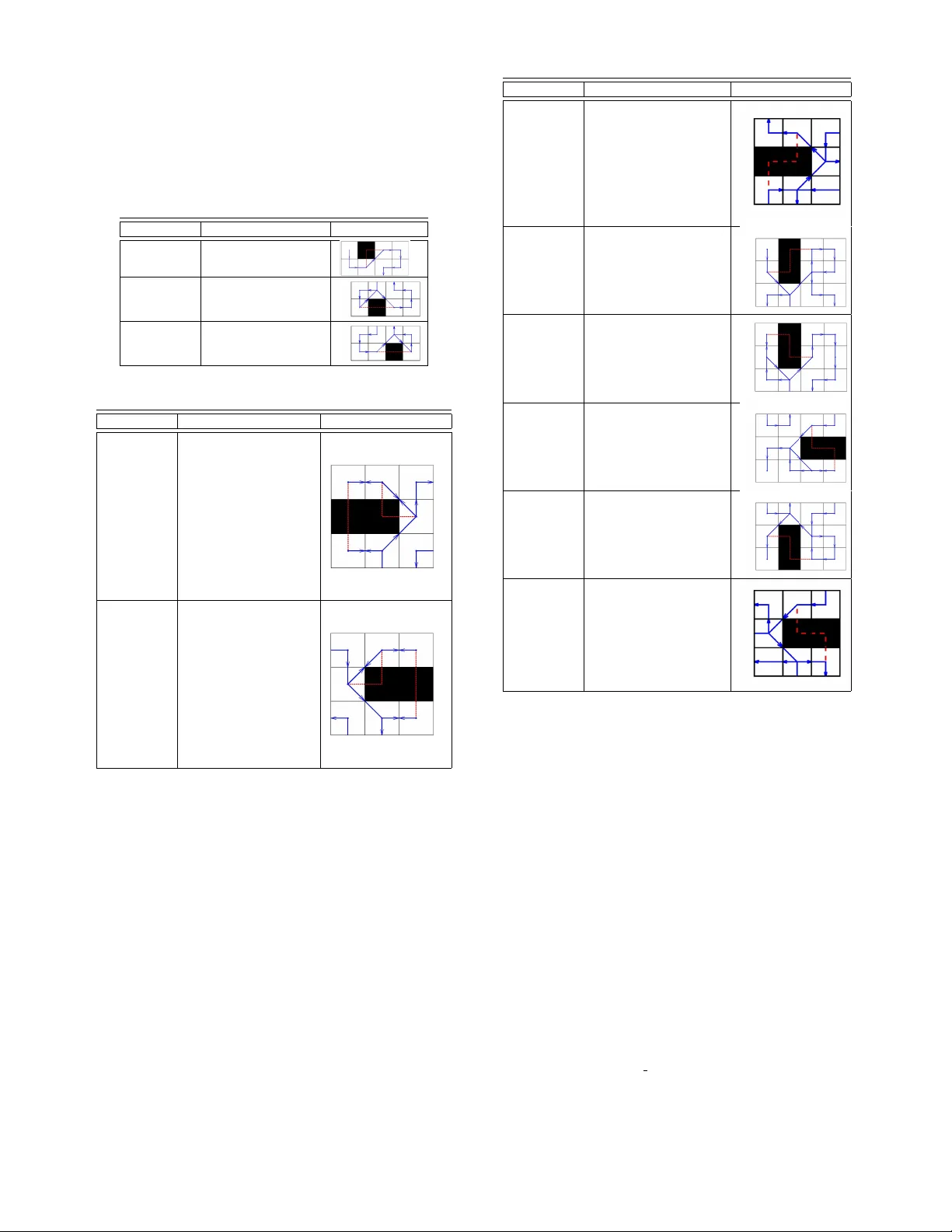
Modification of Hilbert’ s Space-Filling Curv e to A void Obstacles: A Robotic Path-Planning Strategy Anant A. Joshi 1 , Maulik C. Bhatt 2 and Arpita Sinha 3 Abstract — This paper addresses the pr oblem of exploring a region using Hilbert’s space-filling curve in the presence of obstacles. No prior knowledge of the region being explored is assumed. An online algorithm is proposed which can implement evasi ve strategies to avoid up to two obstacles placed side by side and successfully explore the entire region. The strategies are specified changing the waypoint array follo wed by the r obot, locally at the hole. The fractal nature of Hilbert’ s space-filling curve has been exploited in proving the validity of the solution. Extension of algorithm for bigger obstacles is briefly shown. I . I N T RO D U C T I O N A space-filling curve is a one-dimensional curve which passes through ev ery point of an N-dimensional region [1]. Rigorously , it is a continuous mapping from [0 , 1] to an n -dimensional Euclidean space which has a positiv e n - dimensional Jordan content [2]. In 1891, D. Hilbert proposed Hilbert’ s space-filling curve (hereby referred to as HC). The HC has interesting properties which are exploited in various applications. Being a space-filling curve it covers all points in a two-dimensional square space. This intrinsic property of all space-filling curves attracts many applications where an area needs to be cov ered by an agent like tool path planning [3], area coverage problems [4] and optimization problems where HC is used to con vert a multi-dimensional problem to a one dimension [5]. It has a locality preserving property by virtue of which images of points that are close to each other, are also close to each other [6], [7], [8]. Locality preservation is sought after in computer science applications inv olving parallel computing, data storage and indexing of meshes [7], [9], [10], [11]. Its fractal nature allows us to zoom in and out of the curve and still obtain the same pattern. This inspires application to search problems where the space to be explored has patches which are more interesting or crucial than others [12]. The fractal nature of the HC is exploited to explore patches of higher interest at a higher le vel of refinement resulting in higher resolution of observation. There is a myriad of literature addressing robotic search and path planning problems [13]. HC finds its application in this area too by virtue of its attractiv e properties which lead to nov el and interesting solutions to conv entional problems [1], [12]. Howe ver , both consider an environment without any obstacles for the robotic agent. Problems considering the robotic exploration of a space containing obstacles, along a space-filling curve are interesting, because it may not always 1 Undergraduate Student, Mechanical Engineering; 2 Undergraduate Student, Aerospace Engineering; 3 Associate Professor, Systems and Control Engineering; Indian Institute of T echnology Bombay , In- dia. { anantjoshi,maulik.bhatt,arpita.sinha } @iitb.ac.in (a) (b) Fig. 1: (a) Strategy for single node([15]) (b)Strategy fails be trivial to find a path around the obstacles and continue on the curve. [14] presents a solution to such a problem using a Sierpinski curve but this method requires knowledge of the domain to be explored in advance. A solution which can be implemented online would be a welcome candidate for an autonomous agent. W e consider the problem of robotic exploration, i.e., of finding a path for an autonomous agent to traverse, such that it is able to e xplore a given region fully . W e employ the HC in this endeav our . Such an online strategy is presented in [15], which divides the space into a grid based on the sensor resolution of the agent, and plans a path when the obstacle occupies one grid square. If there is a bigger obstacle, these strategies are unable to guarantee evasion (for eg. fig. 1). W e extend this w ork by considering obstacles of bigger size and establishing online ev asion strategies for the same. W e rely on fractal nature of the HC and exploit the grammar [7] of the HC to design and verify our strategies. W e redefine the methods presented in [15] since, with some modifications, they are able to ev ade holes with two blocked nodes. W e w ork under the assumption that two squares in the grid are blocked. The techniques presented in this work can be extended to other space-filling curves by using the grammar of those curves. W e present simulation and hardware experiments to demonstrate our strategies. I I . P R E L I M I NA R I E S A. Mathematical Preliminaries In this paper , we will be dealing with the HC which maps from the unit interval I = [0 , 1] to the unit square Q = [0 , 1] × [0 , 1] . I is first divided into four equal sub- intervals which are mapped onto four congruent sub-squares of Q such that adjacent sub-interv als map to adjacent sub- squares. Repeating this process on the sub-interv als and corresponding sub-squares for N iterations produces a HC of order N . On repeating this procedure infinitely , the complete HC is generated [2]. W e use an approximated v ersion of the HC [15] (Fig. 2). For an N th order HC, 4 N points in I namely λ i = i 4 N for i = 0 , 1 , 2 ... 4 N − 1 are used. Under the approximation used, these points are mapped to the centre- points of the subsquares obtained when Q is divided into 4 N congruent sub-squares. Every node maps to a unique subsquare and likewise, ev ery subsquare corresponds to a (a) (b) Fig. 2: Approximated (a)first (b)second order HC L 0 :=  0 1 1 0  L 1 :=  1 0 0 1  L 2 := − L 0 L 3 := − L 1 T ABLE I: Maps defining HC Grammar unique node. The images of these points in Q will be referred to as nodes of the N th order HC. Any node of an N th order HC will be addressed by node number defined to be the inde x of the point in I which maps to that subsquare. For instance, the node number of the subsquare to which λ 2 maps is 2, and this node will be addressed as ‘node 2’. The HC being a fractal can have exactly four possible orientations denoted by H , A , B , C (fig. 3a, 3b, 3c, 3d respec- tiv ely) [7]. A HC of one orientation can be transformed into another by rotation and reflection using the maps L 0 , L 1 , L 2 and L 3 giv en in table I. When we refer to any HC, we refer to it’ s H orientation by default, unless otherwise specified. Remark 1: L T i L i = I hence L i r epresent either r otation or r eflection for i = 1 , 2 , 3 , 4 ( I is the identity matrix). In fig. 2 it can be seen that the second order curve is made up of 4 first order curves suitably transformed using table I. This property along with a finite number of possible orientations for an HC (fig. 3) highlight the fractal nature of the HC. Due to this fractal nature any HC of order N 1 can similarly be constructed from 4 N 1 − N 2 HC of order N 2 ( N 1 > N 2 ). Thus, intuitiv ely any higher order HC can be thought to be composed of lower order HC. Nodes can be classified as corner or non-corner nodes [15]. Corner nodes are nodes which enter or exit any first order HC. Node 0 and node 3 are corner nodes in Fig. 2a. One more classification is introduced, where 5 types of nodes are defined called τ 1 , . . . , τ 5 . The procedure to check the type of the node is as follows: suppose i is the node number of the node in concern. Define two vectors: one as a vector( # » v 1 ) from ( i − 1) th node to i th node and the other as a vector( # » v 2 ) from i th node to ( i + 1) th node. Define r := # » v 1 · # » v 2 | # » v 1 || # » v 2 | to be used in the classification. % will be used for the mathematical operator mod (modulo). τ 1 : r < 1 τ 2 : r = 0 τ 3 : r > 0 τ 4 : r = 1 τ 5 : r < 0 T ABLE II: Sets based on path passing through the node B. T erminology Used The natural or der of the HC refers to the HC follo wed in ascending order of its nodes. The distance between any two nodes n 1 , n 2 defined as d ( n 1 , n 2 ) will be the Euclidean distance between them. The obstacle blocking the nodes is referred to as a hole . T wo nodes are said to be edge connected (a) (b) (c) (d) Fig. 3: H , A , B , C orientations of a first order HC Fig. 4: Possible ways to enter and exit a hole if they share a common edge and vertex connected if the sub- squares share a common vertex but not a common edge. The neighbours of a node is the set of all those nodes which are edge connected or vertex connected to it. A hole is said to hav e been evaded if all nodes of the HC e xcept those blocked by the hole are cov ered. An evasion strate gy describes a path to successfully ev ade a hole. I I I . M A I N R E S U LT A. Pr oblem F ormulation The problem of a robotic agent on an exploration task moving on the nodes of an N th order HC in Q = [0 , 1] × [0 , 1] is considered, in the presence of obstacles. It is assumed that the sensing range of the agent is limited to the neigh- bouring nodes of the agent’ s current node. It is assumed that the obstacle cov ers two or fewer nodes of the HC. An online algorithm is presented to implements strategies that ev ade the blocked nodes. The e vasion strategies make sure that all av ailable nodes except the ones blocked by the obstacle are cov ered by the agent and that the agent exits Q at the last node of the HC. It will be assumed that for a HC of order N , the first node, which is node 0 (also called entry node) and the last node, which is node 4 N − 1 (also called exit node) of the HC are av ailable otherwise the agent cannot enter and exit the curve. B. Pr oposed Solution to Evade upto T wo Blocked Nodes Evasion strategies hav e been proposed to ev ade the holes under consideration. When a hole is detected, a detour is planned that takes the agent around the hole and puts it back on the HC. The detour strategies are presented in tables V to VII. The strategies modify the order in which the HC is trav ersed. T able V contains strategies from [15] to ev ade a single blocked node, but suitably modified for our application. If there are two blocked nodes, they may be edge connected, verte x connected or not connected at all. For the latter two cases, ev asion is done by strategies in table V (as we show further). For edge connected nodes, we begin by identifying how the hole may be entered or exited in a normal HC (fig. 4 which shows blocked nodes in yello w and paths in blue). W e see that the hole can be entered via one of 6 ways e 1 through e 6 and exited via E 1 through E 6 . e 7 is used only when both the blocked nodes are consecutiv e. This gives us a hint of how to devise ev asion strategies for these cases. Some of these cases can be ev aded by strategies of V (for eg. e 2 , e 7 , E 2 ) as we sho w further . Howe ver , it is clear that others cases (for eg. e 2 , e 7 , E 3 ) require the de velopment of some new strategies. T able VI and VII contain these new proposed strate gies. Finally , an algorithm is presented to implement these strategies. A n 2 = n 1 + 1 B n 2 = n 1 + 2 C n 2 = n 1 + 3 D n 2 ≥ n 1 + 4 T ABLE III: Sets based on node number difference C. V alidity of Solution W e will consider a HC of order N in this subsection. It will be assumed that nodes 0 and 4 N − 1 are av ailable, that is, if a node n b is assumed to be blocked, n b / ∈ { 0 , 4 N − 1 } . W e will first restate the main result of [15] and highlight some of its properties. s Lemma 1: If there is a hole comprising a single blocked node( n b ) in the HC, there always exists a path from node n b − 1 to node n b + 1 . This path passes only though edge connected neighbours of the blocked node. Pr oof: Any single blocked node n b can be ev aded by strategies described in table V, which by virtue of their construction use only edge connected neighbours of the blocked node.  From the grammar of the HC, nodes n b + 2 and n b − 2 can never be edge connected to n b . Thus, from lemma 1 av ailability of nodes n b − 2 and n b + 2 is not required in any of the ev asion strategies of table V. The ev asion strategies do not use nodes n ≤ n b − 4 or n ≥ n b + 4 . The figures in table V provide an illustration. W e proceed to the case when holes consist of two blocked nodes n 1 and n 2 ( n 1 < n 2 ). T o begin, we di vide them into four sets (T able III) based on the difference in node number . Holes falling in B and D and a certain subset of those falling in C can be ev aded by the strategies in table V. Lemma 2: Holes consisting of exactly two blocked nodes n 1 and n 2 in (i) B or (ii) D can be ev aded by strategies described in table V. The nodes between the blocked nodes will also be covered. Pr oof: W e claim that for both cases n 1 and n 2 can individ- ually be ev aded by strategies in table V. W e will prove this by showing that all nodes required for ev asion are indeed av ailable. n 2 = n 1 + 2 ⇒ n 1 − 3 < n 1 < n 2 < n 1 + 3 ⇒ n 1 + 3 and n 1 − 3 are av ailable in both cases. Thus a path from n 1 − 1 to n 1 + 1 exists ev ading n 1 . Similarly , n 2 − 3 and n 2 + 3 both av ailable ( n 2 − 3 < n 1 < n 2 < n 2 + 3 ) in both cases so a path from n 2 − 1 to n 2 + 1 exists ev ading n 1 . In case of B the only node in between is n 1 +1 which is cov ered by the ev asion for n 1 and in case of D all nodes in between are covered since the normal HC if followed in between.  The upcoming result will help us e xploit the grammar of the HC for further proofs. Recall that the orientation O of a first order HC can take one of four v alues H , A , B , C . Lemma 3: Given two consecuti ve first order HC in any N th order HC with orientations O 1 , O 2 ∈ {H , A , B , C } , one of the maps in table I transforms them into two consecutiv e first order HC curves with orientation H , O 3 or O 3 , H with O 3 ∈ {H , A , B , C } preserving the following: (i) The distance between any two nodes is in variant under the transformation (ii) The sequence in which the nodes are trav ersed (iii) A corner node and non-corner node will continue to re- main a corner node and a non-corner node respectively (a) HH (b) HA (c) HB (d) HC Fig. 5: Combinations of two connected second order HC Similarly , H , O 3 can be transformed into O 1 , O 2 using the in verse transformation while preserving the same properties. Pr oof: A HC of any orientation can be transformed into a HC of any other orientation using the maps in table I [7]. W e choose a map L such that L ( O 1 ) = H . Then O 3 := L ( O 2 ) ∈ {H , A , B , C } . Or we choose L such that L ( O 2 ) = H then O 3 = L ( O 1 ) . Since L i represents pure rotation or reflection for all i , which does not change distances between points, the distance between any two nodes is inv ariant under the transformation. Under any of the transformations, the order in which the nodes are traversed does not change since they are just rotations or reflections, hence nodes which enter or exit the first order HCs continue to do so thus corner nodes remain corner nodes and similarly for non-corner nodes. Similarly , H , O 3 can be transformed to O 1 , O 2 using L T (in verse of L ).  For n 1 , n 2 ∈ A quite a fe w cases can be ev aded using the strategies from table V. In table IV we will sub-di vide A into subcases using fig. 4. a 1 , a 2 , a 3 , a 4 can be e vaded using table V and a 5 requires strategies from table VII. a 1 : ( e 1 , E 2 ) , ( e 1 , E 3 ) , ( e 4 , E 5 ) , ( e 4 , E 6 ) a 3 : ( e 3 , E 3 ) , ( e 2 , E 2 ) a 2 : ( e 2 , E 1 ) , ( e 3 , E 1 ) , ( e 5 , E 4 ) , ( e 6 , E 4 ) a 4 : ( e 1 , E 1 ) , ( e 4 , E 4 ) a 5 : ( e 2 , E 3 ) , ( e 3 , E 2 ) , ( e 5 , E 6 ) , ( e 6 , E 5 ) T ABLE IV: Subcases of A Lemma 4: (i) Holes in a 5 can be ev aded using table VII (ii) Holes in a 1 , a 2 , a 3 , a 4 can be ev aded using table V Pr oof: (i) First we will claim that both n 1 and n 2 belong to the same second order HC. Assume they don’t, which means either n 2 %16 = 0 or n 1 %16 = 15 . Assume n 1 %16 = 15 . Now we will need to check all possible cases of two neighbouring second order HC to confirm this. Ho wev er, due to its grammar [7] we need only check finite number of cases. From lemma 3 we need only check the four cases when the last node of a H orientation second order HC is blocked, and the next second order curve is of H , A , B , C orientation. Fig. 5 provides an illustration. It can be observed that in none of them, is the hole created of a 5 type. Checking similarly for n 2 %16 = 0 shows the claim. W e will prove the main result by claiming that all nodes required for ev asion are available. W e will show the av ail- ability of nodes in questions using HC grammar, lemma 3 and table VII. It can be seen from table VII that n 1 %16 ∈ { 0 , 2 , 6 , 8 , 12 , 14 } . For n 1 %16 ∈ { 2 , 6 , 8 , 12 } the proof is immediate by looking at a single second-order HC since all required for e vasion are in the same-second order HC and av ailable (refer table VII). For n 1 %16 = 14 , we will look at all possible combinations of 2 connected second-order HC. W e will assume that the hole blocks the last 2 nodes of the first second-order curve and check whether the nodes required for ev asion are av ailable. Howe ver , we again need only check cases H H , AH , BH , C H since all others can be con verted to these using lemma 3. The case in question occurs only in the AH or B H case and the nodes required for ev asion are av ailable. This can be proven on the exact same lines for n 1 %16 = 0 hence result is proven for a 5 . (ii) Suppose we would like to show the result for a 1 . For two nodes n 1 and n 2 in A , either they both are in the same first order HC or in neighbouring first order HC, with n 1 being node 3 in the first one and n 2 being node 0 in the second one. If n 1 and n 2 are in the same first-order HC, then they must satisfy n 1 %4 = 0 , n 2 %4 = 1 . In this case the nodes required for ev asion are av ailable. T o analyse the case when they’ re in neighbouring first order curves, similar to (i) check cases of neighbouring first order HC of orientations HH , HA , HB , H C . It is seen that the nodes required for ev asion are av ailable. Hence result is prov en for a 1 and can be proven similarly for the rest.  W e will no w establish a few facts (to be used in the content that follows) about two blocked nodes n 1 and n 2 in C . W e will assume N ≥ 2 since if N = 1 (i.e. first order HC) then n 1 = 0 and n 3 = 3 which is not allowed since by assumption they are av ailable. An N th order HC comprises 2 2 N − 2 first order HC. Let n 1 lie in the N th F first order curve. W e will assume N F < 2 2 N − 2 in lemma 5 since if N F = 2 2 N − 2 then n 2 = 4 N − 1 which must be av ailable, by assumption. Lemma 5: Consider two nodes n 1 and n 2 in C as follows: assume N ≥ 2 and let n 1 lie in the N th F first order curve with N F 6 = 2 2 N − 2 . n 1 mod4 ∈ { 0 , 1 , 2 , 3 } and corresponding to each value: (i) If n 1 %4 = 0 then n 2 lies in N th F first order curve itself. They both are corner nodes and edge connected. (ii) If n 1 %4 = 1 then n 2 lies in ( N F + 1) th first order curve. n 1 is a non-corner node and n 2 is a corner node and they are not edge connected. (iii) If n 1 %4 = 2 then n 2 lies in ( N F + 1) th first order curve. They both are non-corner nodes. (iv) If n 1 %4 = 3 then n 2 lies in ( N F + 1) th first order curve. n 1 is a corner node and n 2 is a non-corner node and they are not edge connected. Pr oof: (i) Observe that n 1 and n 2 are the entry and exit nodes of a first order HC respectiv ely , hence the result is established directly from the structure of a first order HC. W e will use the following in further proofs: 1) If a node n lies in the N th F first order curve and n %4= k then n = k + 4( N F − 1) 2) For two nodes to be edge connected, the distance between them should be precisely equal to d 0 units. (ii) n 2 = 3 + 1 + 4( N F − 1) = 4 N F + 0 hence n 2 lies in ( N F + 1) th first order curve. Assume that the N th F first order HC is of H orientation. The distances between n 1 and n 2 is d 0 for all orientations H , A , B , C of the ( N F + 1) th curve. If N th F HC is of a different orientation than H , transform it into H orientation (lemma 3) and this transformation does not change distances between nodes. Hence n 1 and n 2 are not edge connected. n 1 mod4=1, n 2 mod4 = 0 giv es that n 1 (a) Computer Simulation (b) Hardware Experiment Fig. 6: Implementation of Evasion Strategies is a non-corner node and n 2 is a corner node. Proof for (iii), (iv) follo ws similarly .  W e will group items (ii),(iii) and (iv) in the aforementioned list in lemma 5 into c 2 (nodes such that both of them are non- corner nodes or exactly one of them is a corner node) and (i) into c 1 (both corner nodes). Lemma 6: Holes in c 2 can be ev aded using table V. Pr oof: Since n 1 and n 2 = n 1 + 3 are the only blocked nodes, n 1 − 1 , n 1 + 1 , n 2 − 1 and n 2 + 1 are av ailable. a) If node n 1 + 1 is visited, n 2 − 1 will be visited since they are neighbours b) As shown earlier there will exist paths from n 1 − 1 to n 1 + 1 and n 2 − 1 to n 2 + 1 respectively if both are non- corner nodes. c) If exactly one of them is a corner node, consider the case if only n 1 was the blocked node. Then from lemma 1 there exists a path from n 1 − 1 to n 1 + 1 which passes only through edge connected neighbours of n 1 . Ev en though n 2 is blocked, this path will continue to be av ailable since n 1 and n 2 are not edge connected neighbours (lemma 5). Similarly for n 2 a path from n 2 − 1 to n 2 + 1 will exist and be available even though n 1 is blocked. From (a), (b), (c), there exists a path from n 1 − 1 to n 2 + 1 which also covers all nodes in between.  Similarly like A , there exist 2 ways ( e i ) to enter and 2 ways ( E j ) to exit holes in c 1 . In the following lemma, we will employ a similar approach as lemma 4. Lemma 7: Holes in c 1 can be ev aded by using table VI. Pr oof (Sketch): From lemma 5 the hole lies entirely in a single first order HC. W e will look at all possible cases when such a hole occurs in a second order HC. For n 1 %16 ∈ { 4 , 8 } all nodes required for ev asion are observed to be av ailable. For n 1 %16 ∈ { 0 , 12 } analysing neighbouring second order HC, similar to lemma 4, shows the result.  Theor em 1: A HC having a hole consisting of at most two blocked nodes can be covered using strategies in tables V to VII. Pr oof: Follo ws from lemmas 1, 2, 4, 6 and 7.  Theorem 1 can be easily extended to the case when there are multiple holes, but each hole consists of either a single blocked node, two edge connected blocked nodes or two verte x connected blocked nodes, and that the holes are not edge or vertex connected to each other (fig. 6). I V . I M P L E M E N TA T I O N A. Philosophy and Salient P oints of the Algorithm W e present the algorithm 1 to implement the strategies in tables V to VII. It takes as an input the order of the HC to be tra veled and giv es output an array containing coordinates of all nodes from node zero to the last node. Agent travels in a straight line between any two consecuti ve nodes. It checks if the next node is av ailable or blocked, and commands the agent to either follo w a certain strategy or continue on the HC. The node classification (as in table II) and algorithm design is done so as to ev ade maximum possible holes using strategies for a single blocked node (table V). For the cases when it is not possible, new strategies are introduced in tables VI and VII. One of the examples where one obstacle strategy works is ( e 1 , e 7 , E 3 ) , which can be also seen in the top left corner of the fig. 6a. In that case, the agent detects the obstacle at n th 1 node and uses the strategy from table V to reach ( n 1 + 3) th node. No w , the next node in N is n 2 , it will be a τ 1 node and from our algorithm, it will be skipped and the robot will go to ( n 2 + 1) th node directly . In all the tables N represents the array containing all the nodes of HC which agent has to cover . In table V the blocked node is either skipped or replaced by another av ailable node to ev ade the hole. In tables VI and VII more then one consecutive elements of N is replaced by other av ailable nodes to ev ade the hole. Note that the node classification in table II is not mutually exclusi ve as it is necessary by the virtue of the design of the algorithm. In table VI it might be possible that the number of nodes to be added are more than the number of nodes to be replaced. In such cases. nodes which are already cov ered are replaced and the value of n is decreased in order to preserve the total number of elements in N . Computer simulation of ev asion strategies is shown in fig. 6a, where multiple holes have been considered in a HC of order 3. B. Experimental V alidation The implementation of the proposed algorithm was done in a similar manner to that of [16]. The implementation was done on a ground differential drive robot F irebir d V . The experiments were conducted in a motion capture en vironment using 8 VICON V antage V5 cameras. The data from VICON cameras goes into the HP R  Z-440 workstation. The V icon T racker V ersion 3.4 softw are in w orkstation extracts the position of the robot and broadcasts it into the local W i- fi. T o access this data we use vicon-bridge node in ROS. It makes the data av ailable in pose feedback form. The controller for the robot is run as nodes in a ROS Indigo Igloo en vironment in Ubuntu 14.04 on a Lenovo R  Z51-70 Laptop (Intel R  Core i7-5500U CPU, 2.4GHz and 16 GB RAM). Communication between laptop and F ir ebird V is done using Xbee R  modules. In order to avoid further comple xity in detecting the obstacles, the location of the obstacles were known to the set up apriori but it was made available to the node which runs the algorithm only when the agent reaches in the neighbourhood of the blocked node. W e model the robot hardware using unicycle kinematics ˙ x = v ( cos ( ψ )) , ˙ y = v ( sin ( ψ )) , ˙ ψ = ω . W e get the current state as feedback from vicon bridge node in R OS. Let the desired state be ( x d , y d , ψ d ) . The desired state is computed in bot controller node equipped with algorithm 1 (written in Python) running in ROS. Then, real-time input of linear velocity ( v ) and angular velocity ( ω ) to the robot is given as following: v = k 1 p ( x d − x ) 2 + ( y d − y ) 2 and ψ d = tan − 1  y d − y x d − x  , ω = k 2 ( ψ d − ψ ) . The values of k 1 and k 2 are 1 and 1.8 respectiv ely . W e performed two experiments [17], [18] (web-links). Results of [18] are portrayed in fig. 6b. Algorithm 1 HC Modification to ev ade obstacles 1: Input : N = order of HC 2: Output : Array N of nodes from N (0) to N (4 N − 1) 3: Initialize : n = 0 4: while n ≤ 4 N − 1 do 5: Initialize n 1 = n 6: if n 1 is blocked then 7: if n 1 ∈ τ 1 then 8: Initialize n 2 = n 1 + 1 9: if n 2 is blocked and n 2 ∈ τ 2 then 10: if The combination, ( n 1 , n 2 ) , can be clas- sified according to table VII then 11: Use the strategy described in table VII 12: Break 13: else 14: n ← n + 1 15: Break 16: else if n 1 ∈ τ 3 then 17: Use the strategy described in table V 18: Break 19: else 20: n ← n + 1 21: Break 22: else if n 1 ∈ τ 4 then 23: if n 1 %2=0 then 24: Initialize n 2 = n 1 + 3 25: if n 2 is blocked then 26: Use the strategy described in table VI 27: Break 28: else 29: Use the strategy described in table V 30: Break 31: else if n 1 %2=1 then 32: Initialize n 2 = n 1 − 3 33: if n 2 is blocked then 34: Initialize n 2 = n 1 35: n 1 ← n 1 − 3 36: Use the strategy described in table VI 37: Break 38: else 39: Use the strategy described in table V 40: Break 41: else 42: Pass 43: else 44: Pass 45: V isit N ( n ) 46: n ← n + 1 V . C O N C L U S I O N S The problem of exploring a re gion with holes using the HC has been considered. The holes are assumed to covers two or fewer nodes of the HC and an online algorithm is presented which implements strategies that e vade any such obstacle. T o prov e the e vasion of nodes, the fractal nature of the HC has been exploited. Computer simulations and hardware experiments demonstrate tractability of proposed algorithm. Extension of algorithm with more blocked nodes is sho wn through numerical simulation and hardware experiments. Node T ype Change in Path Figure n b ∈ τ 2 ∪ τ 5 n ← n − 1 n b ∈ τ 3 n b %2 = 1 N ( n b ) ← N ( n b − 3) n b ∈ τ 3 n b %2 = 0 N ( n b ) ← N ( n b + 3) T ABLE V: Ev asion Strategies for Single Blocked Node ( n b ) n is as used in algorithm 1 Node T ype Change in Path Figure n 1 ∈ τ 4 n 2 ∈ τ 2 n 1 %2 = 0 n 2 = n 1 + 3 d 1 := d ( n 1 + 4 , n 1 − 2) d 2 := d ( n 1 + 4 , n 1 − 4) if( d 1 < d 2 ) N ( n 1 − 1 , ..., n 1 + 3) ← N ( n 1 − 2 , n 1 + 4 , n 1 + 2 , n 1 + 1 , n 1 + 2) n ← n − 1 elif( d 1 > d 2 ) N ( n 1 − 1 , ..., n 1 + 3) ← N ( n 1 − 4 , n 1 + 4 , n 1 + 2 , n 1 + 1 , n 1 + 2) n ← n − 1 n 1 ∈ τ 2 n 2 ∈ τ 4 n 2 %2 = 1 n 2 = n 1 + 3 d 1 := d ( n 2 − 4 , n 2 + 2) d 2 := d ( n 2 − 4 , n 2 + 4) if( d 1 < d 2 ) N ( n 2 − 2 , ..., n 2 ) ← N ( n 2 − 2 , n 2 − 4 , n 2 + 2 ) n ← n − 2 elif( d 1 > d 2 ) N ( n 2 − 2 , ..., n 2 ) ← N ( n 2 − 2 , n 2 − 4 , n 2 + 4 ) n ← n − 2 T ABLE VI: Strategies for n 2 = n 1 + 3 n is as used in algorithm 1 R E F E R E N C E S [1] S. V . Spires and S. Y . Goldsmith, “Exhaustive geographic search with mobile robots along space-filling curves, ” Collective Robotics , pp. 1– 12, 1998. [2] H. Sagan, Space-Filling Curves . Springer-V erlag, New Y ork, 1994. [3] M. Bertoldi, M. Y ardimci, C. Pistor, and S. Guceri, “Domain decom- position and space filling curves in toolpath planning and generation, ” Solid Fr eeform F abrication Pr oceedings , pp. 267–276, 1998. [4] Z. Liu, Y . Chen, B. Liu, C. Cao, and X. Fu, “Hawk: An unmanned mini helicopter-based aerial wireless kit for localization, ” Pr oceedings of IEEE INFOCOM , 2012. [5] B. Goertzel, “Global optimization with space-filling curves, ” Applied Mathematics Letters , vol. 12, no. 8, pp. 133–135, 1999. [6] C. Gotsman and M. Lindenbaum, “On the metric properties of discrete space-filling curves, ” IEEE Tr ansactions on Image Processing , vol. 5, no. 5, pp. 794–797, May 1996. [7] M. Bader , Space-Filling Curves: An Intr oduction with Applications in Scientific Computing . Springer-V erlag Berlin Heidelberg, 2013. [8] K. E. Bauman, “The dilation factor of the peano-hilbert curve, ” Mathematical Notes , vol. 80, no. 5, pp. 609–620, Nov 2006. [9] G. Chochia, M. Cole, and T . Heywood, “Implementing the hierar- chical pram on the 2d mesh: analyses and experiments, ” in Proceed- ings.Seventh IEEE Symposium on P arallel and Distributed Processing , Oct 1995, pp. 587–594. Node T ype Change in Path Figure n 1 ∈ τ 1 n 2 ∈ τ 2 n 1 %16 = 0 n 2 = n 1 + 1 d 1 := d ( n 1 + 14 , n 1 − 4) d 2 := d ( n 1 + 14 , n 1 − 2) if( d 1 < d 2 ) N ( n 1 , n 1 + 1) ← N ( n 1 − 4 , n 1 + 14) elif( d 1 > d 2 ) N ( n 1 , n 1 + 1) ← N ( n 1 − 2 , n 1 + 14) n 1 ∈ τ 1 n 2 ∈ τ 2 n 1 %16 = 2 n 2 = n 1 + 1 N ( n 1 , n 1 + 1) ← N ( n 1 + 11 , n 1 + 5 ) n 1 ∈ τ 1 n 2 ∈ τ 2 n 1 %16 = 6 n 2 = n 1 + 1 N ( n 1 , n 1 + 1) ← N ( n 1 − 2 , n 1 − 4) n 1 ∈ τ 1 n 2 ∈ τ 2 n 1 %16 = 8 n 2 = n 1 + 1 N ( n 1 , n 1 + 1) ← N ( n 1 + 5 , n 1 + 3) n 1 ∈ τ 1 n 2 ∈ τ 2 n 1 %16 = 12 n 2 = n 1 + 1 N ( n 1 , n 1 + 1) ← N ( n 1 − 4 , n 1 − 10) n 1 ∈ τ 1 n 2 ∈ τ 2 n 1 %16 = 14 n 2 = n 1 + 1 d 1 := d ( n 1 − 13 , n 1 + 5) d 2 := d ( n 1 − 13 , n 1 + 3) if( d 1 < d 2 ) N ( n 1 , n 1 + 1) ← N ( n 1 − 13 , n 1 + 5) elif( d 1 > d 2 ) N ( n 1 , n 1 + 1) ← N ( n 1 − 13 , n 1 + 3) T ABLE VII: Strategies for n 2 = n 1 + 1 [10] B. Moon, H. Jagadish, C. Faloutsos, and J. H. Saltz, “ Analysis of the clustering properties of the hilbert space-filling curve, ” IEEE T ransactions on Knowledge & Data Engineering , vol. 13, pp. 124– 141, 01 2001. [11] R. Niedermeier , K. Reinhardt, and P . Sanders, “T owards optimal locality in mesh-indexings, ” Discrete Applied Mathematics , vol. 117, no. 1, pp. 211 – 237, 2002. [12] S. A. Sadat, J. W awerla, and R. V aughan, “Fractal trajectories for on- line non-uniform aerial coverage, ” Pr oceedings of IEEE International Confer ence on Robotics and Automation (ICRA) , 2015. [13] E. Galceran and M. Carreras, “ A survey on coverage path planning for robotics, ” Robotics and Autonomous Systems , vol. 61, no. 12, pp. 1258 – 1276, 2013. [14] A. T iwari, H. Chandra, J. Y adegar , and J. W ang, “Constructing optimal cyclic tours for planar exploration and obstacle avoidance : A graph theory approach, ” in Advances in Cooperative Contr ol and Optimization . Springer Berlin Heidelberg, 2007, pp. 145–165. [15] S. H. Nair , A. Sinha, and L. V achhani, “Hilbert’ s space-filling curve for regions with holes, ” in 2017 IEEE 56th Annual Confer ence on Decision and Control (CDC) , Dec 2017, pp. 313–319. [16] A. V . Borkar, V . S. Borkar, and A. Sinha, “ Aerial monitoring of slow moving conv oys using elliptical orbits, ” Eur opean Journal of Contr ol , vol. 46, pp. 90–102, 2019. [17] https://youtu.be/G7AZaYn66xA. [18] https://youtu.be/75qi3zcZ dM.